General Linear Threshold Models with Application to Influence Maximization
Abstract
A number of models have been developed for information spread through networks, often for solving the Influence Maximization (IM) problem. IM is the task of choosing a fixed number of nodes to “seed” with information in order to maximize the spread of this information through the network, with applications in areas such as marketing and public health. Most methods for this problem rely heavily on the assumption of the known strength of connections between network members (edge weights), which is often unrealistic. In this paper, we develop a likelihood-based approach to estimate edge weights from the fully and partially observed information diffusion paths. We also introduce a broad class of information diffusion models, the general linear threshold (GLT) model, which generalizes the well-known linear threshold (LT) model by allowing arbitrary distributions of node activation thresholds. We then show our weight estimator is consistent under the GLT and some mild assumptions. For the special case of the standard LT model, we also present a much faster expectation-maximization approach for weight estimation. Finally, we prove that for the GLT models, the IM problem can be solved by a natural greedy algorithm with standard optimality guarantees if all node threshold distributions have concave cumulative distribution functions. Extensive experiments on synthetic and real-world networks demonstrate that the flexibility in the choice of threshold distribution combined with the estimation of edge weights significantly improves the quality of IM solutions, spread prediction, and the estimates of the node activation probabilities.
Keywords: Social Networks, Influence Maximization, Information Diffusion Models, Linear Threshold Model
1 Introduction
The emergence of large-scale online social networks has led to a new surge of interest in information diffusion models. These networks supply incredibly rich data, which can include connections between users, user covariates, e.g., demographics, and the paths of information propagation between users, e.g., retweets or reposts. Information diffusion paths, also known as propagation traces, are especially valuable in modeling information spread since they provide direct data on the influence users have on their network neighbors. “Information” in this context can be interpreted broadly and refer to anything that can spread from node to node, be it a news item or a virus (and sometimes these are connected – Dinh and Parulian (2020) showed that the spread of Covid-19 through people’s social networks can be well predicted by their interactions around Covid-related posts on Twitter). For example, Liu and Wu (2018) used propagation traces for fake news detection while Saito et al. (2008) proposed to estimate information diffusion probabilities from the same data. Goyal et al. (2011) proposed a model assigning credits to users based on how well they propagate information and subsequently using these weights to solve the influence maximization (IM) problem, that is, identifying the best “seed nodes” for spreading information. While the IM problem and spread prediction are the main applications of the present paper, the method we propose for estimating edge weights from propagation traces is general and can be applied to any other downstream problem in network analysis after the weights are estimated, such as testing for network differences (Tantardini et al., 2019) or community detection in weighted graphs (Lancichinetti and Fortunato, 2009).
Since the IM problem was formulated by Richardson and Domingos (2002) and formalized by Kempe et al. (2003), many efficient approaches for identifying the best seed sets have been proposed. All of them require a probability model for how information (“influence”) spreads over the network, known as the diffusion model, usually with edge- or vertex-specific parameters governing information spread. Perhaps the most popular is the independent cascade (IC) model (Goldenberg et al., 2001), which assumes that each edge is associated with a transmission probability and all transmission events are independent. Another popular choice is the linear threshold (LT) model (Granovetter, 1978)), which assumes that each edge has a deterministic weight and each node uses a uniformly distributed random threshold to decide whether to “accept” incoming information; this will be stated formally in Section 2. There is substantial literature on solving the IM problem given a specific diffusion model (see Banerjee et al. (2020) for a survey), and some on more efficient but less general approaches, for example, mixed integer programming for the IC model (Farnad et al., 2020). However, in most applications, the underlying diffusion parameters are unknown and can significantly change the IM problem solution under misspecification. Work by Goyal et al. (2011) highlighted this issue, showing that the IM solutions improve significantly when the edge weights are estimated, for example using the EM approach of Saito et al. (2008) for the IC model. One contribution we make in this paper is to develop an EM approach analogous to Saito et al. (2008) for edge weight estimation under the LT model (Section 4.6). However, the LT and IC model classes are not especially rich, and the natural next step would be to estimate the parameters of more sophisticated and flexible network diffusion models. While there are well-known flexible generalizations of these two models, such as the triggering and general threshold (GT) models studied in Kempe et al. (2003), their additional flexibility is achieved at the cost of exponentially many additional parameters (see Proposition 3.1), making parameter estimation impossible with realistic amounts of data. To address this, we propose the general linear threshold (GLT) model, which has only parameters but is much more flexible than the LT model; importantly, it allows for heterogeneity in how readily users accept new information. Our generalization is a special case of the GT model but not of the triggering model. We propose a likelihood-based approach for estimating its parameters and show the estimator is consistent under mild regularity conditions. In Section A.6 of the Appendix, we extend this technique by showing the IC model parameters are identifiable and can be consistently estimated under similar conditions. While there have been several papers (He et al., 2016; Narasimhan et al., 2015) establishing Probably Approximately Correct (PAC) learnability guarantees for nodes’ activation probabilities under the IC, LT, and several similar models, surprisingly, there has been very little work establishing theoretical guarantees for the diffusion model parameters. The only paper we are aware of that addresses these questions is the work by Rodriguez et al. (2014) where authors derive identifiability conditions and establish consistency for the parameters of several continuous-time diffusion models. In such a way, to the best of our knowledge, this work is the first one to prove consistency for the estimates of discrete diffusion model parameters based on the propagation traces. Finally, we show that under some additional conditions on the GLT model, the IM problem under the GLT assumption can be solved by the natural and widely used greedy strategy described in Section 2, with standard optimality guarantees.
The rest of this manuscript is organized as follows: in Section 2, we briefly introduce the background on the IM problem and the relevant diffusion models and fix notation. In Section 3 we propose the Generalized Linear Threshold (GLT) model, describe its relationship to other diffusion models, and derive the conditions under which the IM problem under the GLT model can be optimally solved by the greedy strategy. In Section 4, we establish identifiability conditions, derive a likelihood approach to weight estimation under the GLT model, and establish consistency. We also present an EM-based improvement of our estimation algorithm for the standard LT model. Finally, Section 5 presents experiments on synthetic and a real-world network showing that using the proposed weight estimation procedure outperforms standard heuristics and estimating the threshold distributions under the GLT model instead of using the standard LT model can substantially improve the IM solutions.
2 Background
In this section, we formally define the influence maximization problem and the most commonly used diffusion models. We start by setting up notation.
Let be a graph where is the set of nodes and is the set of edges. Unless otherwise stated, we assume throughout this manuscript that is a directed graph with no loops and repeated edges. Denote the sets of parent and children nodes of a node as, respectively,
Similarly, for any set of nodes , let
In words, and consist of nodes outside of which have at least one child or parent in , respectively.
A diffusion model associated with controls the spread of information over the graph. In general, the information diffusion process starts with a given non-empty set of initially activated (influenced) nodes, also known as the seed set. Then, at each time step , a new subset of nodes , which were not previously active, become activated following the diffusion model. We only consider progressive propagation, which means that once a node is activated, it remains activated (i.e., it never forgets the information it received). This assumption implies that all sets are disjoint. Let be the set of all nodes activated by time . We also assume that if a node was not active at time , it cannot be activated at time unless one of its parent nodes was newly activated at time , meaning that if a given subset of active parents was once not enough for activation, it will never be enough in the future. In particular, this means that a node cannot be influenced from outside of the network or self-activated. The process stops when no new node is activated; that time point is denoted by }. The entire diffusion process can be described by the set sequence , which is called a propagation trace, or an information diffusion path. For convenience, we let and (no nodes are active before the information is seeded). Finally, we write to denote the set of all nodes activated by the end of the propagation described by .
The assumptions on the diffusion process imply not every sequence of node subsets can be a feasible propagation trace. The feasibility condition can be formulated as follows:
Definition 1 (Feasible trace).
We say that a set sequence with is a feasible propagation trace if
-
1.
is not an empty set;
-
2.
All sets are disjoint;
-
3.
For every , each newly activated node has at least one parent in , i.e., .
The set of all feasible traces on will be denoted by . Now we are ready to state a formal definition of a diffusion model.
Definition 2 (Diffusion model).
A diffusion model on is a mapping which takes any feasible trace on as input and outputs a probability distribution on the feasible sets of newly active nodes:
The mapping depends on parameters , which can depend on .
When the context is clear, we will omit the subscript and write . This definition does not specify the distribution that generates the seed set ; instead, it conditions all output distributions on it. If we additionally define a distribution over the subsets of which does not depend on , satisfies , and assume that the seed set is drawn from and then passed on to the diffusion model, it will be convenient to refer to the pair as a seeded diffusion model with the seed distribution . When and are clear from the context we will write instead.
A seeded diffusion model naturally implies a distribution on all the feasible traces:
Definition 3 (Trace distribution under the seeded diffusion model).
Consider a simple directed graph and a seeded diffusion model on it. For each feasible trace consider the transition probabilities . Then the following probability mass function defines the distribution of feasible traces on induced by :
On the other hand, the trace distribution also uniquely defines the diffusion model. Indeed, for any feasible trace and , we can write:
| (1) |
where denotes the indicator of an event.
Next, we give definitions of the two most popular diffusion models, the Linear Threshold (LT) and the Independent Cascade (IC) models. Conceptually, under the LT model, all of a node’s activated parents influence it additively, whereas the IC model gives each active parent node one individual chance to influence its children.
Definition 4 (Linear Threshold (LT) Model).
Assume that each edge has a weight , and the in-degrees satisfy, for all ,
| (2) |
Each node has an activation threshold , with thresholds sampled i.i.d. from the distribution at the outset. At every time step , each non-active node becomes activated if the sum of the edge weights from all its previously activated parents exceeds its threshold , that is, if
Definition 5 (Independent Cascade (IC) Model).
Assume that each edge is associated with a propagation probability . At every time step , each newly active node independently tries to activate all its not yet active children with probability . That is, if and at least one , for , takes on the value .
The vector of parameters in the general definition 2 corresponds to for the LT model, and to for the IC model.
Given a graph and an arbitrary diffusion model on it, the Influence Maximization (IM) problem poses a natural question: which nodes are the most effective spreaders of information in the network, that is, where should a given number of seeds be placed to start the diffusion process so that the resulting expected number of activated nodes is maximized? This question was first introduced by Richardson and Domingos (2002) and further formalized by Kempe et al. (2003). Before stating the definition of the IM problem, we introduce the notion of the influence function:
Definition 6 (Influence function).
Given a simple directed graph and a diffusion model on it, let the influence function denote a set function that maps each subset of nodes to the expected number of nodes influenced if propagation is seeded at :
Definition 7 (The Influence Maximization (IM) problem).
Given a simple directed graph , a diffusion model on it, and a budget , the IM problem is to find a subset which would maximize the influence function across all -element subsets of :
For the rest of the paper, we omit the subscripts and of whenever they are clear from the context.
In Kempe et al. (2003), it was shown that the IM problem is NP-hard under both LT and IC models and hence intractable unless . However, when the influence function has certain properties, the optimal solution can be well approximated by a greedy strategy (see Algorithm 1). These properties are monotonicity and submodularity. Monotonicity means that adding more nodes to a seed set cannot decrease the value of the influence function, and submodularity means that adding a node to a given seed set is at least as efficient as adding it to a bigger seed set containing this given set, both very reasonable and mild assumptions.
Definition 8 (Monotonicity).
An influence function is monotone if for any .
Definition 9 (Submodularity).
An influence function is submodular if for any and .
Though Kempe et al. (2003) were the first to study the greedy algorithm behavior in the context of the IM problem, the analysis of its worst-case performance under monotonicity and submodularity assumptions dates back to the works of Nemhauser, Wolsey, and Fisher who proved the following result:
Theorem 2.1 (Cornuéjols et al. (1977) and Nemhauser et al. (1978)).
Consider a universal set and a monotone and submodular function . Let of size be the set obtained by selecting elements from one at a time, when at each step one chooses an element that provides the largest marginal increase in the value of . Let be the true maximizer of over all -element subsets of . Then
| (3) |
or, in other words, provides a approximation to the optimal .
Kempe et al. (2003) showed that under the LT and IC models, the influence function has the monotonicity and submodularity properties and thus the IM problem under these models can be solved by Algorithm 1 with the optimality guarantee in (3).
3 The general linear threshold model
In this section, we introduce a generalization of the LT model which we call the General Linear Threshold (GLT) model. It generalizes the standard LT model by allowing each node to have an individual and possibly non-uniform threshold distribution . We show that for GLT models with concave ’s, Algorithm 1 solves the IM problem with the optimality guarantees (3). We further show that despite having only parameters, the GLT model is surprisingly rich. In particular, in Proposition 3.2, we show that it is not a special case of the Triggering model, a well-known overparametrized generalization of the LT model. We begin by giving a formal definition of the GLT model.
Definition 10 (General Linear Threshold (GLT) Model).
Assume each node is assigned a non-negative threshold from a distribution with cumulative distribution function (cdf) , s.t. and . Also, assume that each edge is assigned a weight , such that for all ,
The propagation process is then the same as for the LT model.
An even more general model was introduced by Kempe et al. (2003), allowing the activation probability to be an arbitrary, not necessarily linear, function of the active parent set.
Definition 11 (General Threshold (GT) model).
Assume each node in the graph is assigned a threshold function that maps subsets of ’s parents to , such that . As in the LT model, each node chooses an activation threshold . A node is activated at step if .
The GLT model is an instance of the GT model with . The GT model does not automatically guarantee the desirable submodularity property, which implies the IM problem cannot be solved by Algorithm 1 with the optimality guarantee (3). However, Mossel and Roch (2010) showed that a relatively mild extra assumption enforces submodularity on the GT model.
Theorem 3.1 (Mossel and Roch (2010)).
The GT model on a graph is monotone and submodular if the threshold function is monotone and submodular for each node .
We will denote the subclass of Monotone Submodular GT models by MSGT. Theorem 3.1 implies a sufficient submodularity condition for the GLT model, stated next.
Theorem 3.2.
The GLT model on a graph is monotone and submodular if the threshold cdf is concave for each node .
The proof can be found in Section A.3 of the Appendix. This general theorem makes it easy to establish conditions on a particular threshold distribution that guarantee submodularity. For example, if the thresholds are sampled from a beta distribution (to which we will return later), it is easy to check submodularity, as shown next in Corollary 3.1.
Corollary 3.1.
A GLT model with is submodular if for all .
Proof.
The density of the distribution is non-increasing on its support whenever for each
which is equivalent to . ∎
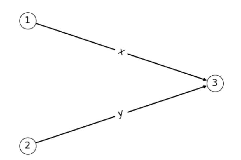
The following example shows submodularity may fail for a network instance under the GLT model when the threshold cdfs are not concave. Consider the 3-node graph shown in Figure 1. The influence function satisfies and Then if and both edge weights and are positive, the submodularity condition implies a contradiction:
On the other hand, if at least one of and is zero, submodularity will hold.
Next, we compare the GLT model to the LT model and its other widely used generalization from the MSGT family known as the Triggering model. For formal proof showing that the LT model is a special case of the Triggering model, see Theorem 2.5 of Kempe et al. (2003).
Definition 12 (Triggering Model).
At the outset, each node independently chooses a random triggering set according to some distribution over subsets of its parents. An inactive node becomes active at time if its triggering set contains a node in .
The Triggering model allows for a different value of for each non-empty subset of ’s parents, making the number of unknown parameters , which is not feasible to fit in most cases. On the other hand, the LT model has only parameters, so computationally it is an attractive option. A major disadvantage of the LT model is its assumption that all nodes behave identically when receiving equal amounts of influence from their neighbors, and does not allow for heterogeneity in readiness to be influenced. In reality, some people are conservative and need a lot to be convinced, while some may be trusting and easily influenced; this can be estimated from data on propagation traces through that network. The GLT model allows us to account for differences in users’ attitudes to new information while not significantly increasing the number of unknown parameters.
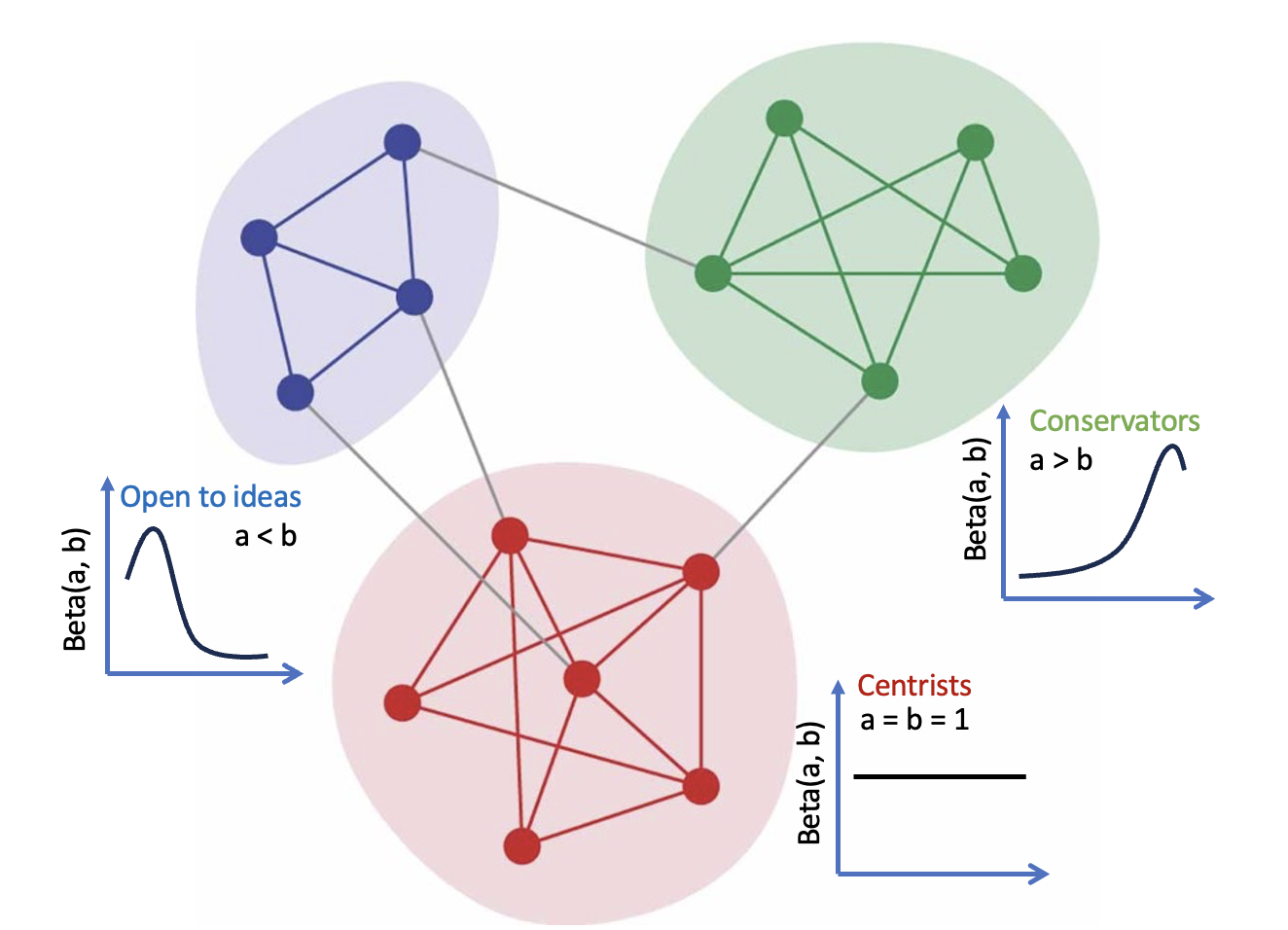
A natural approach to making the number of parameters manageable is to choose threshold distributions from a parametric family. For example, if , the model has only parameters. If we further assume that the network can be partitioned into communities and nodes within one community follow the same distribution (see Figure 2), we can further reduce this number. However, even if each node has its own individual set of parameters, the following proposition demonstrates that the GLT almost always has fewer parameters than the Triggering and the MSGT models, which both have parameters.
Proposition 3.1.
Consider a directed graph with average node in-degree . Then for any ,
Proof.
Noticing that and applying Jensen’s inequality to the convex function , we obtain
∎
The next proposition shows that despite a much smaller number of parameters, there are submodular instances of the GLT model that can not be represented as an instance of the Triggering model. The proof can be found in Section 3.2 of the Appendix.
Proposition 3.2.
There exists a GLT model with a submodular influence function for which there is no instance of the Triggering model such that the induced trace distributions of and coincide on each feasible trace .
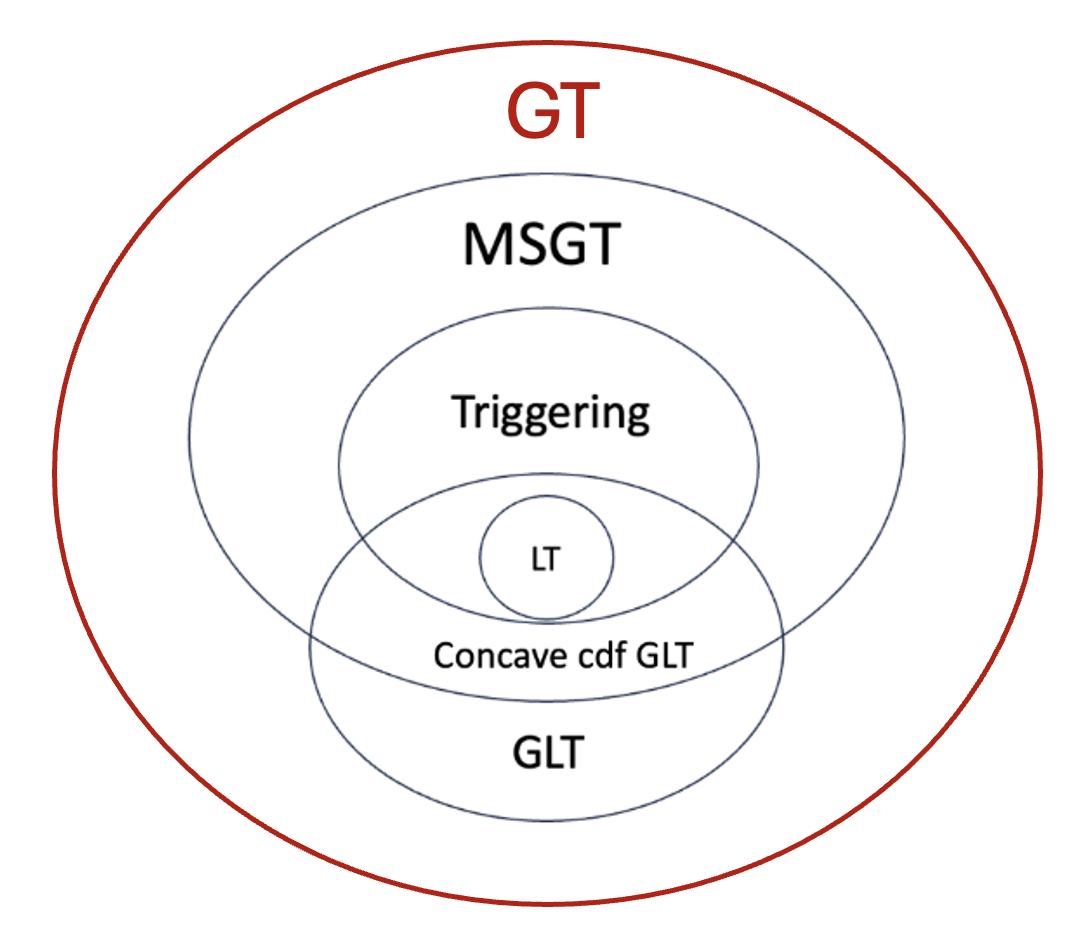
Figure 3 summarizes the relationships between the various diffusion models. As in Proposition 3.2, we represent one diffusion model family as contained in another model family if for each instance of the smaller family there is an instance of the bigger family such that their induced trace distributions coincide.
4 Estimation and theoretical properties under the GLT model
4.1 Identifiability for the GLT model
In this section, we study identifiability of the weights with respect to the trace distribution induced by the GLT model, and then present conditions for consistency of the MLE of the edge weights. To simplify further narration, we would like to fix the edge ordering in to work with as a vector, not as a set. To achieve this, we assume that the nodes are enumerated from to and the edges are sorted in the lexicographical order with the child node having priority. For example, a triangle graph with each edge going in both directions corresponds to the ordered set .
By Definition 3 and independence of node activation thresholds, the probability of a feasible trace is given by
| (4) |
where denotes the influence node receives from a set , i.e.,
| (5) |
The first term in (4) does not depend on by definition of the seeded diffusion model. The second term represents nodes that were not activated but have at least one active parent in the trace. The third term captures information about activated nodes, i.e., nodes in .
The parameter space includes all weights satisfying the GLT model assumptions,
| (6) |
This space has a nice block structure arising from grouping edges by their terminal node. Denote the set of (child) vertices with at least one parent as
| (7) |
and for every , define its individual parameter subspace as
| (8) |
where denotes the -norm of a vector and inequality between a number and vector denotes element-wise comparison. Then, the parameter space can be written as a Cartesian product of individual parameter spaces:
| (9) |
This decomposition will be crucial for deriving the MLE of weights since it allows decomposing the log-likelihood optimization problem into at most small sub-problems.
To ensure identifiability of , we need to impose some constraints on the threshold cdfs , which up to this point were not restricted.
Assumption 1.
For each , the threshold cdf is continuous, strictly monotone (thus invertible), and .
Together with stated in the GLT model definition, implies the threshold distributions have bounded support. This will be crucial in proving the MLE consistency since it makes the parameter space compact. Additionally, we will assume that all the weights are separated from zero and each node in-degree is separated from the upper bound of the corresponding threshold distribution:
Assumption 2.
There exists a universal , such that the true weights satisfy for all and for all .
Intuitively, Assumption 1 means that any node has a positive chance to activate its child even if none of the child’s other parents are activated. Assumption 2 means that even if all parents of a node are activated, there is a positive probability the node will not be activated. We require because if all then it should also hold
We rule out equality because it would force for all . Assumption 2 implies that similarly to (9), we can define the truncated parameter space as where
| (10) |
The following property of is crucial for identifiability.
Lemma 4.1.
Under Assumption 1, any feasible trace with has a positive probability w.r.t. for each .
Proof.
Fix an arbitrary . For any with parent subsets , the strict monotonicity of implies
Therefore, each term of the product in (4) is strictly positive. As the number of terms in the likelihood is bounded by (each node can appear in a trace at most once), we have . ∎
The next proposition shows that even if all weights are separated from zero, identifiability is not guaranteed if there are source nodes that have zero probability of appearing in the trace.
Proposition 4.1.
If is identifiable, then for each with , the following must hold for any :
If additionally, it must hold that
Proof.
Assume there is and with a child such that . Since cannot be activated, the edge will never participate in a trace, therefore if we change while keeping other weights in fixed, will remain the same. Contradiction. Now, if also does not have a parent, it cannot be activated by other nodes, so it may appear in only if it lies in a seed set. ∎
Next, we show that the necessary condition in Proposition 4.1 has an equivalent more intuitive formulation.
Proposition 4.2.
Define a set of "reachable" nodes in that consists of s.t. either or there is a directed path to from at least one with . Then the following conditions are equivalent:
-
(a)
For all , it holds ,
-
(b)
There is such that .
-
(c)
.
Proof.
Statement (a) trivially implies (b). To show (b) implies (c), note that (b) implies that there is a feasible trace with and . We prove by induction over that there is a path to from a node . First, for , since is feasible, should have a parent in . Now suppose the induction hypothesis holds for . If there is a path to from , there is also a path from since should have a parent in by feasibility. This results in a path connecting and which implies that .
To prove (c) implies (a), consider an arbitrary . If , then (a) holds. Assume now there is a sequence of nodes such that for all and with . Then, is a feasible trace that has a positive probability for any according to Lemma 4.1. ∎
Combining Propositions 4.2 and 4.1, we deduce that weights are identifiable only if all edges have sources either appearing in or reachable from a seed set having positive probability, i.e., if . Unfortunately, the following example demonstrates this condition is insufficient for identifiability.
Example.
Consider the graph in Figure 1 and assume that the seed set is fixed at nodes 1 and 2, i.e., . Then the distribution of possible traces is a function of ,
and therefore and are not identifiable, only their sum is. It is easy to verify that if the support of includes at least two distinct subsets of , the weights are identifiable.
This example provides some intuition on why identifiability of imposes some requirements on the seed set distribution . This intuition is formalized in the following theorem. Its proof is given in Section A.4 of the Appendix.
Theorem 4.1.
Under Assumption 1, is identifiable if and only if for each child node with , there exist such that
-
1.
For each , there is a feasible trace with , , and .
-
2.
The matrix is invertible.
4.2 Weight estimation under GLT models
Next, we propose a likelihood-based approach to estimating the weights in the GLT model from a collection of observed (and therefore feasible) propagation traces,
| (11) |
where is the number of time steps in trace . For now, we assume that all threshold distributions are known and postpone the discussion of estimating the threshold distribution to Section 4.5.
We assume that the trace collection is i.i.d., by which we mean
-
(a)
Seed sets are generated independently from the seed distribution ;
-
(b)
Node thresholds are generated independently for each trace and for each node, with
For an i.i.d. trace collection, the parameters can be estimated by solving the problem
| (12) |
where , the log-likelihood of the trace , by (4), takes the form
| (13) | ||||
Here, we omitted the term as it does not depend on . Note that in (12), we optimize over untruncated space instead of , as in practice the true "slack" variable from Assumption 2 is unknown.
Examining (13), we see that the likelihood depends only on weights for , the subset of child nodes defined by
| (14) |
Here, each set in the union consists of the nodes that either were activated after the seed set within a given trace or failed to be activated while having an active parent.
This is still a large number of parameters to optimize over, but fortunately, the problem has a block structure we can use to speed up computations. By changing the order of summation, we can rewrite the objective of (12) as
where
| (15) |
and is the activation time of node in trace . Therefore, solving (12) is equivalent to maximizing over defined in (8), for each , an optimization problem with only variables and affine constraints:
| (16) |
The next natural question is whether this optimization problem is convex. The feasible set is a convex simplex, and the arguments of in (4.2) depend linearly on . Thus is a concave function of if is a concave function on . For example, if is uniformly distributed on , as in the standard LT model, then is concave. This turns out to be true for all distributions with log-concave densities, and in particular when is the Beta distribution with parameters and .
Proposition 4.3.
The function in (4.2) is concave in if has a log-concave density.
The proof is given in Section A.1 of the Appendix.
4.3 Consistency
If the identifiability conditions hold, MLE consistency follows almost immediately from standard results.
Theorem 4.2.
Proof.
By Theorem 9.9 in Keener (2010), MLE is consistent if the parameter space is compact, is a continuous function of for each , is identifiable, and
| (17) |
The parameter space is compact as a closed subset of compact . Continuity of holds since each term in (13) is a composition of continuous functions. The last condition holds since the quantity under the supremum (17) is a continuous function of , therefore it achieves its maximum at some . Finally, and have the same support by Lemma 4.1, therefore the quantity under the expectation is finite for any in the support of . ∎
As the weight identifiability condition in Theorem 4.1 is very restrictive, Theorem 4.2 becomes hardly applicable in practice. Therefore, we conclude this section by extending the consistency result to the case when some edges have source nodes unreachable from a seed set in the support of . One possible way to deal with this issue is to restrict the identifiability question to a subgraph where all source nodes are reachable. Instead of the full graph , we can define a restriction , where is the set of nodes reachable from or belonging to a seed set in the support of and , and restrict the parameter space to as follows:
Then Theorems 4.1 and 4.2 are both applicable to the subgraph .
We note that the identifiability conditions stated in Theorem 4.1 are also necessary and sufficient for identifying the IC model parameters, assuming all edge probabilities are bounded away from zero and one. Given identifiability, the proof of consistency is identical to Theorem 4.2. Since the IC model lies outside of the main scope of this paper, we present and prove the corresponding theorems in Section A.6 of the Appendix.
4.4 Extension to partially-observed traces.
In many real-life applications, we do not observe a full propagation trace but only have access to a node’s active parents it had before activating itself. For example, suppose a person (node) gets infected given their other family members (parent nodes) are currently infected. In that case, we can infer that the virus transmission from one of the family members occurred while we may not know the full virus propagation path leading to their own infection. We will encode each such observation for node as a pair where is a set of ’s active (infected) parents and is an indicator of the event that together managed to activate (infect) . We will refer to such pair as a pseudo-trace.
Suppose that for each child node , we observe a possibly empty collection of pseudo-traces
| (18) |
that we would like to use to estimate the GLT weights . A natural question is if we can assume some pseudo-trace generating distribution for so that the corresponding likelihood optimization problem and consistency theory directly follow from what we previously established for the fully observed traces. The most straightforward way to do that is to treat a pseudo-trace as a trace seeded at and propagating in a graph with nodes and edges . Given that , the feasible traces on can only be of two types: those who stopped immediately at the seed set and those who activated at time one and then stopped. The first case corresponds to a pseudo-trace and the second one to . Assuming that the sets are independently generated from a parameter-free seed distribution supported on the subsets of , the pseudo-trace likelihood will have the form
| (19) |
Aggregation of these probabilities across all pseudo-traces in results in the log-likelihood:
| (20) |
where we omitted the parameter-free terms. The assumption that the seed distribution does not depend on any diffusion model parameters may seem strong, as a seed node in could have been activated by its own network parents, making the probability of indirectly dependent on the seed’s incoming edge weights. However, by carefully comparing (20) with its counterpart for fully observed traces in (4.2), we observe that the only difference is that, in the latter case, we always subtract under the logarithm for traces where was activated. This term represents the probability that the active parent set preceding the one that eventually activated was not enough for ’s activation. Thus, the only information lost in a pseudo-trace, compared to a fully observed trace, is which parent subset of an influenced node was not sufficient to activate it.
With pseudo-trace distribution formulated as a trace distribution on a sub-graph , identifiability and consistency theory are extended straightforwardly:
Theorem 4.3.
Under Assumption 1, is identifiable for with if and only if there exist such that
-
1.
For each , it holds .
-
2.
The matrix is invertible.
Theorem 4.4.
Proofs of these theorems can be found in Section A.5 of Appendix.
4.5 Estimation of threshold parameters
So far we have treated threshold distributions known, while they are unlikely to be observed in reality. While we cannot estimate these parameters without assuming something about their distribution, we can easily obtain an estimate if we assume each comes from the same parametric family with parameters . For example, assuming , we can define with to satisfy conditions in both Corollary 3.1 and Proposition 4.3. Then we can estimate for each by solving the following optimization problem:
| (21) |
where the individual node likelihood is the one from (4.2) with the Beta distribution cdfs plugged in. Allowing to vary within the feasible set makes the optimization problem non-convex even in the simplest case of a one-parameter family. Thus finding even a local optimum of (21) requires careful tuning of the gradient steps since and might have very different magnitudes. A natural way to deal with that problem is to switch to coordinate gradient descent, alternating between fixing one set of variables ( or ) and optimizing over the other one. Our numerical experiments, however, showed that this type of coordinate gradient descent converges reliably only if the initial values are sufficiently close to the truth (not included in the paper but available in the GitHub repository). Therefore, unless the dimension of is very high, we choose from a discrete grid, optimize (21) over for each and choose the one resulting in the highest log-likelihood. An example of such optimization when all node thresholds follow the same distribution (with unknown) can be found in the Section B.1 of Appendix. While in our further experiments, we also assume that all nodes’ thresholds follow Beta distribution, the parametric family as well as the parameter grid in (21) are not required to be the same across .
Unfortunately, if we add more threshold parameters to the model, the grid search approach quickly becomes computationally infeasible. A possible alternative is the method of Turnbull (1976), who proposed a non-parametric estimator of the cdf from a set of intervals within which the corresponding (censored) random variable was independently observed. In the GLT model case, for each node , we observe independent realizations of its activation threshold, each within a weight-dependent interval. This interval is for traces where was activated, and for traces where it was not. This suggests a natural iterative procedure that alternates solving (16) separately for each and estimating nonparametrically. We leave investigation of this method for future work.
4.6 EM-algorithm for the LT model
Though each problem in (16) has only optimized variables, it may still be a large number when the network is sufficiently dense. In this case, efficient optimization may require significant computational resources. Thus, we present a much faster Expectation-Maximization (EM) algorithm for weight estimation under the LT model that uses explicit parameter updates avoiding numerical gradient computation. This method is analogous to the approach of Saito et al. (2008), who derived an EM algorithm under the independent cascade (IC) model. A simulation study comparing the run time and estimation accuracy of the EM algorithm with problem (16) can be found in Section B.2 of Appendix.
By Theorem 2.5 in Kempe et al. (2003), the LT model can be equivalently reformulated in terms of the Triggering model as follows.
Definition 13 (Equivalent definition of the LT model).
Assume we are given a graph with non-negative edge weights satisfying the LT model constraint for all . Suppose that at the start each node independently chooses its triggering node set which contains at most one parent node . Each parent is chosen to be in with probability , and with probability . Given the initial seed set , at each time step , a node is activated () if .
This formulation has the advantage of a natural latent structure which can be leveraged to derive an EM algorithm. For each trace, define latent variables
where is the indicator of the event that chooses as its activator in trace . Then the full joint log-likelihood for and the trace can be written as
where
To perform the -step, we need to compute the conditional expectation of given the trace and the current estimate of the weights . First, consider the case when and . Then
where the denominator gives the probability that is activated at time along the trace , i.e., the probability that ’s one chosen activating node is in the set . Next, for , we have
Finally, if chose an activating node that was not activated along the trace, i.e., if and , we have
Summing over all the traces , we obtain the following target function for the -step of the EM algorithm:
| (22) |
To perform the -step, we solve the system of linear equations given by the optimality condition . The system can be split into blocks of equations, with each block only involving . Solving this for each explicitly leads to the update for the weight
| (23) |
where
| (24) | ||||
| (25) |
Note that if was activated in each trace where it had at least one active parent. In this case, (23) implies , as expected (in-degree achieves the maximum possible value).
The resulting EM optimization procedure can be summarized as Algorithm 2. Similarly to problem (16), this algorithm can be parallelized w.r.t. the child nodes since the update rule for depends only on its previous iteration estimate but not on the whole .
5 Experiments
In this section, we present simulation studies and a real-world data example to illustrate the effectiveness of the proposed method. The code for these analyses is available at https://github.com/AlexanderKagan/gltm_experiments. The parameter estimation algorithms for the IC (Saito et al. (2008)), LT (Algorithm 2), and GLT (16) models, as well as trace sampling, spread estimation, and greedy algorithm under these models, are implemented as a Python package InfluenceDiffusion, available at https://github.com/AlexanderKagan/InfluenceDifusion. Whenever we fit the GLT model by solving the optimization problem in equation (16), we use the SciPy implementation of the SLSQP solver (Jones et al., 2001). For all synthetic graphs in subsequent experiments, seed sets are sampled uniformly from the node sets of sizes between 1 and 5:
| (26) |
5.1 Weight estimation under the LT model
We begin by demonstrating that Algorithm 2 outperforms existing heuristics for weight estimation when the LT model is used as the ground truth for trace generation. While solving problem (16) with all set as uniform distributions is a possible alternative, we do not include it in the comparison because its weight estimates are identical to those of the EM algorithm, up to numerical precision. Therefore, we only report the results for the EM algorithm method (denoted as LT-EM in the plots).
As benchmarks, we use two heuristics from Goyal et al. (2011) and the EM-based method from Saito et al. (2008), which estimates the edge probabilities for the IC model:
-
1.
Weighted Cascade (WC): The weight of an edge is estimated as the inverse of the in-degree of , i.e., .
-
2.
Propagated Trace Proportion (PTP): The weight of edge is estimated based on the ratio between the number of traces where is activated before and the number of traces where is activated. Normalization is used to ensure that the in-degree of each node equals 1:
-
3.
IC probabilities estimated with the EM method from Saito et al. (2008) (IC-EM): Since the estimated edge probabilities in the IC model do not necessarily satisfy the in-degree constraint of the LT model, we normalize them to ensure unit in-degrees:
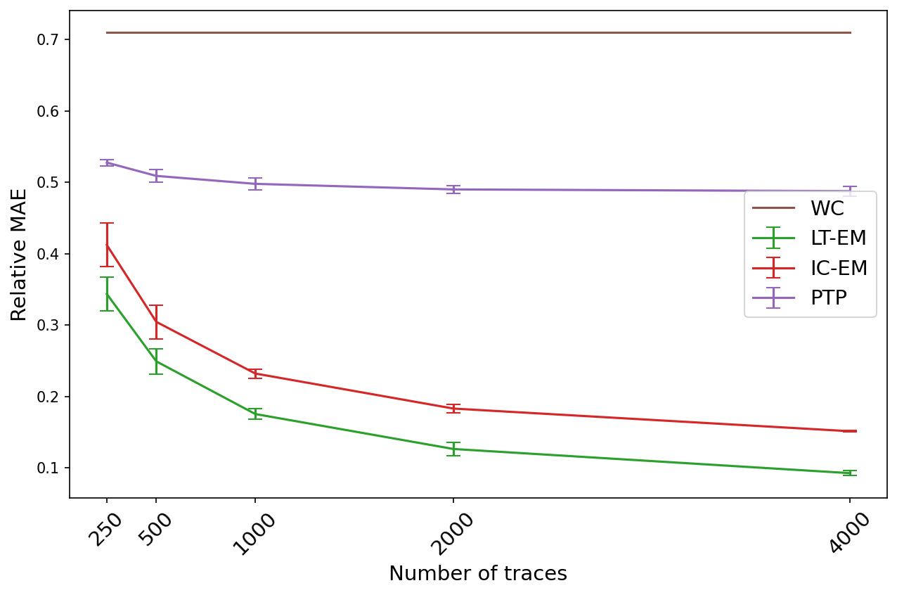
It is important to note that the listed benchmarks can only produce weight estimates where each child node has a unit in-degree. In contrast, Algorithm 2 is not constrained by this restriction due to the term in the update rule, which allows it to fit arbitrary node in-degrees. In our first scenario, we demonstrate that this flexibility significantly improves estimation accuracy when the true node in-degrees differ from one. To create heterogeneous in-degrees, the parent edge weights for each child node are sampled uniformly from the interior of the simplex :
| (27) |
which allows us to evaluate the performance of Algorithm 2 under conditions of varying node in-degrees.
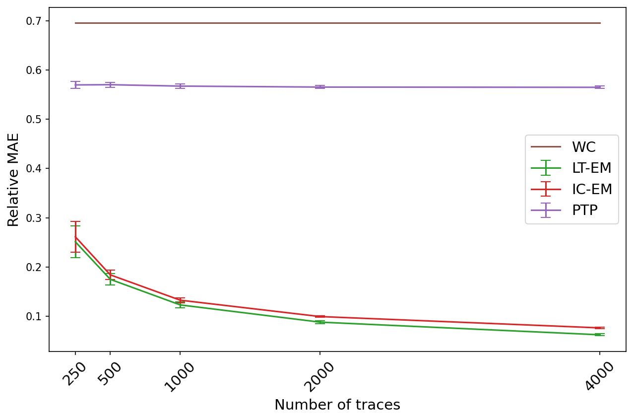
In our second scenario, we show that even when the true node in-degrees are all one, the LT-EM algorithm still significantly outperforms the heuristics PTP and WC, while performing comparably to IC-EM. This experiment also highlights that although Theorem 4.2 guarantees consistency only when node in-degrees are separated from one (as per Assumption 2), in practice, the estimation error decreases towards zero as the number of traces increases, even when this assumption is violated. To generate the ground-truth LT model weights with unit in-degree, we sample uniformly from the surface of the simplex :
| (28) |
which ensures that the generated weights adhere to the unit in-degree constraint for this experimental setting.
In both scenarios, we use a synthetic graph with nodes generated from the directed Erdös-Renyi (ER) model (Erdös and Rényi, 1959), where each directed edge has a probability of . Then given the ground-truth LT model weights, we sample traces, where takes values from , , , , }, and estimate the weights using all candidate methods based on these traces. For each value of , we calculate the Relative Mean Absolute Error (RMAE) between the true weights and estimated weights :
| (29) |
This process is repeated 10 times for each value of . The average RMAEs, along with the corresponding two standard errors, are presented in Figure 4. As shown, the error for the proposed LT-EM approach decreases toward zero as the number of traces increases, and LT-EM consistently outperforms the benchmark methods.
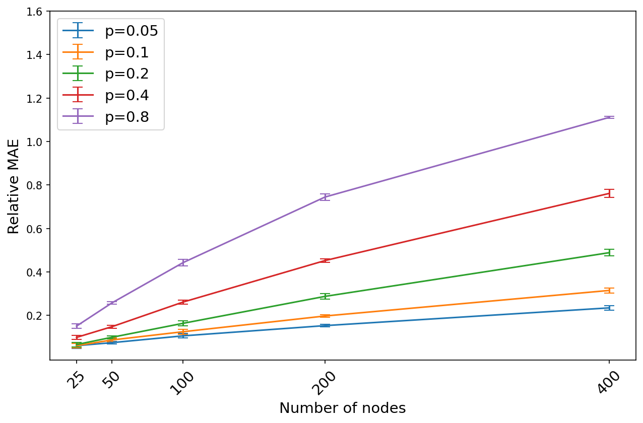
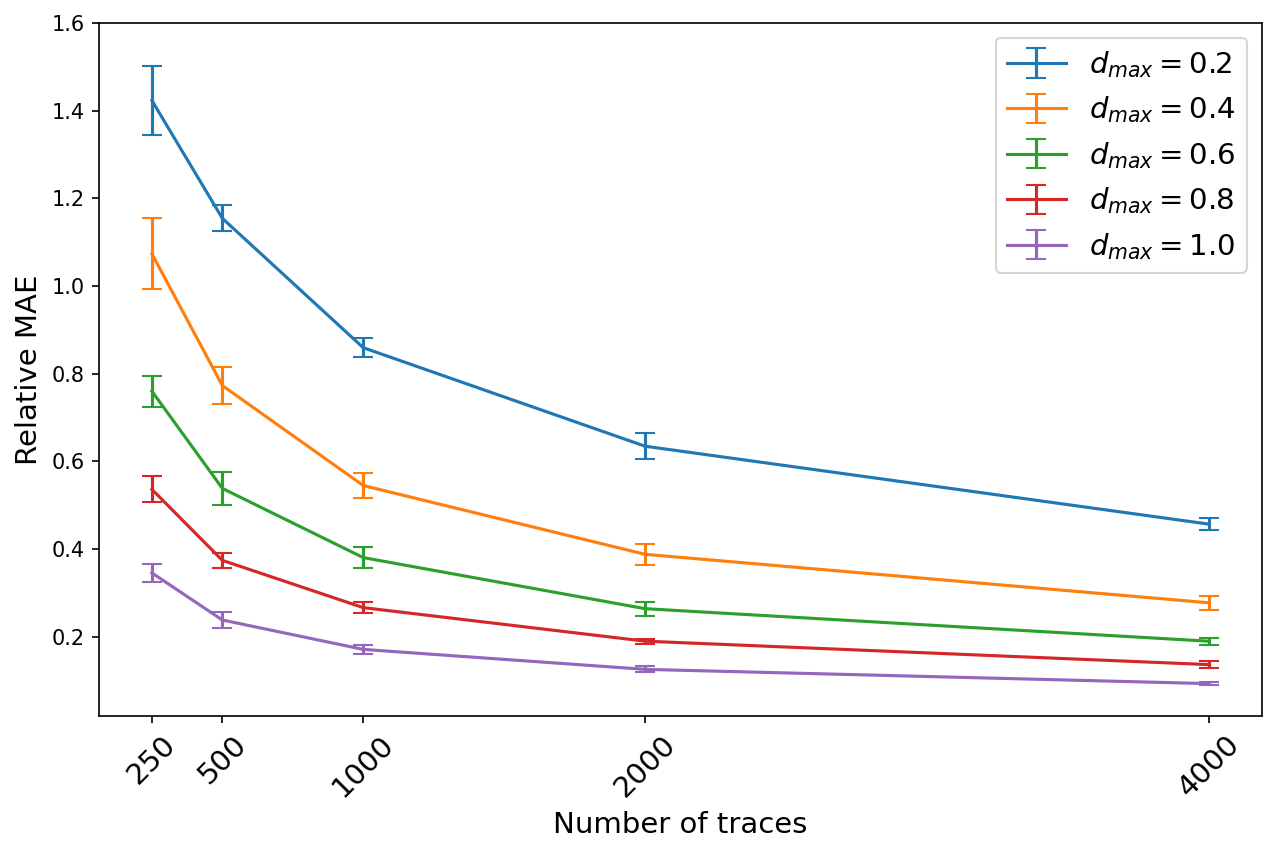
Further, we evaluate the performance of LT-EM under varying ER edge probabilities and different magnitudes of LT model weights. Specifically, in the ER edge probability experiment, we fix the number of traces at while varying the number of graph nodes and the edge probability . In the LT model weight magnitude experiment, we fix the graph size to 100 nodes and , and vary the number of traces and the maximum weighted in-degree of the nodes. The maximum in-degree is controlled by sampling LT model weights using the following procedure:
| (30) |
where . The results are presented in Figure 5. We did not include the benchmark methods in this figure, as their behaviors are similar to those in Figure 4. In the left panel of Figure 5, we observe that the estimation error increases as the edge probability or the network size grows. This is expected, as higher network density or larger network size increases the number of edge weights to estimate, requiring more traces for accurate estimation. The right panel of Figure 5 shows that lower ground-truth weight magnitudes lead to higher estimation errors. This is because larger weight magnitudes result in higher node activation probabilities, producing longer traces with more edge weights contributing to the likelihood estimation.
5.2 The impact of threshold distribution on IM problem solutions
In this section, we demonstrate that selecting an accurate diffusion model can significantly improve the quality of the seed set obtained by solving the IM problem using Algorithm 1.
As in the previous section, we use the directed ER model with to generate graphs with 100 nodes. However, this time we aim to explore the behavior of IM solutions across different network instances, so we sample 10 networks instead of using a fixed network. For each network, we generate traces from the ground-truth GLT model with weights sampled according to (27), and the threshold distributions are as follows:
| (31) |
To examine how diffusion model misspecification impacts IM solutions, we compare the following methods: the LT model with weights estimated by the two heuristics from the previous section (WC and PTP) and Algorithm 2 (LT-EM), the IC model with weights estimated using the method from Saito et al. (2008) (still denoted as IC-EM, though we do not normalize the estimated probabilities here), and the GLT model with both weights and threshold distributions estimated by solving problem (21), where the threshold distribution for each node is assumed to be , with estimated via a grid search over .
For each of the diffusion models described above, we follow these steps:
-
1.
For each network , we estimate the model weights (and in the case of GLT, the values as well) using the corresponding estimation procedure. The estimated diffusion model is denoted , .
- 2.
-
3.
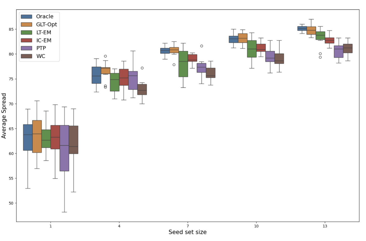
For each network , repeat the above steps five times and calculate the average spread for each seed set size , denoted by .
As a benchmark, we also compute the average spread under the ground truth GLT model, referred to as the Oracle.
Figure 6 presents box-plots (across the 10 networks) of for different values of , ranging from 1, 4, 7, 10, to 13. The results indicate that as the seed set size increases, the choice of diffusion model has a greater impact on the spread. This is likely because, for smaller seed sets, the greedy algorithm tends to select the most central nodes regardless of the fitted model. However, as more non-central nodes are considered for the seed set, significant differences in spread emerge due to the incorrect estimation of their influence by certain models. As expected, LT-EM and IC-EM show inferior performance compared to the ground truth and the GLT model. Notably, the GLT model achieves performance comparable to that of the Oracle.
5.3 Spread estimation
In the previous experiment, we only evaluated the spreads from seed sets that were optimal according to the greedy Algorithm 1. However, in practice, we might also be interested in assessing the spread of information, such as fake news or a virus, initiated from a given seed set that has not been optimally selected. In this section, we show that, for propagation under the GLT model, selecting an accurate threshold distribution can significantly improve the accuracy of spread estimation.
As in the previous experiment, we consider a -node graph generated from the directed ER model with and the associated GLT model, where weights are sampled according to (27) and the threshold distributions are set to for all nodes . We then generate a set of 2500 traces from this GLT model and randomly split them into a training set of 2000 traces and a test set of 500 traces. For candidate threshold distributions , and , we estimate the corresponding GLT model using the training set by solving problem (16) with all set as this distribution. Finally, for each seed set in the test traces, we compute the estimated spread using 1000 Monte Carlo simulations.
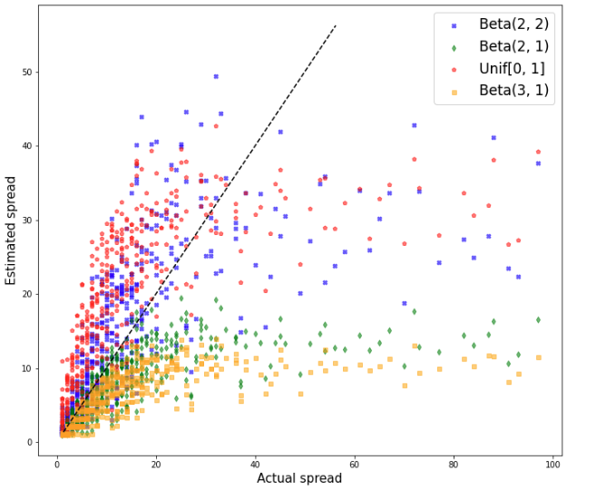
In Figure 7, we observe that the model estimated with the ground-truth distribution performs best maintaining relatively low errors for both low and high true spread values. For example, when the true spread is low, models with (referred to as “conservative” in Figure 2) tend to underestimate the spread, while their “anti-conservative” counterparts tend to overestimate it. For large true spread values, none of the models performs exceptionally well; however, the less conservative models, such as the LT model (red) and the ground truth , show relatively smaller errors. We note that this severe underestimation of spread is not specific to the diffusion models considered in this experiment; rather, it represents a general pattern in spread estimation, as observed in other studies (e.g., Figure 2 in Goyal et al. (2011)). High spread is an extreme event in the tail of the spread distribution and, therefore, cannot be accurately predicted by the mean spread, even when computed under the ground-truth model.
5.4 Real-world data example
In this section, we apply the proposed weight estimation procedures to the Flixster dataset, collected from www.flixster.com, a popular social platform for movie ratings. The dataset contains an undirected, unweighted social network of approximately 1 million users and over 8 million records of the times when users rated specific movies, spanning from 2005 to 2009. Following the notations in Goyal et al. (2011), these rating actions can be encoded as an action log, which is a collection of triples , where represents the user ID, the movie ID, and the time when the user rated the movie. The authors assumed that if user rated movie before user (a connected child in the social graph), the influence likely propagated from to . Of course, this assumption can be questioned, as a user may rate a movie based solely on personal interest or recommendations from someone outside the observed social network. However, the authors’ experiments show that incorporating the information in the action log can significantly improve the estimation of influence propagation. In our experiment, we aim to compare the performance of different diffusion models discussed in this manuscript in terms of their accuracy in predicting node activation events.
To preprocess the data, we first removed all users who rated fewer than 20 movies, as it is difficult to estimate the influence of their social network neighbors on them with limited activity. Next, we apply the periphery-cleaning algorithm described in (Kojaku and Masuda, 2018) to extract the core sub-graph of the remaining users. Finally, we isolate the largest connected component of this core graph. This preprocessing results in a network of 8174 nodes and approximately 50,000 undirected edges. By restricting the initial action log to only the users within this network, we reduce the size of the log to roughly 2.1 million tuples. With the truncated action log in hand, the next step is to transform it into trace or pseudo-trace data that can be used to fit the diffusion models, such as through optimization problem (21) or Algorithm 2. As all diffusion models discussed throughout this manuscript assume a directed graph, we add reverse edges, resulting in 100k directed edges in our final network.
Constructing full propagation traces proves challenging, even in simple scenarios. For example, consider a network with three users who follow each other pairwise and watch the same movie at distinct times . There are already five possible ways to construct the corresponding trace: , or . This complexity arises because the trace data we considered earlier in this manuscript has a discrete-time structure, while the Flixster dataset involves continuous time. To reduce ambiguity in trace construction, we propose using the pseudo-trace framework described in Section 4.4.
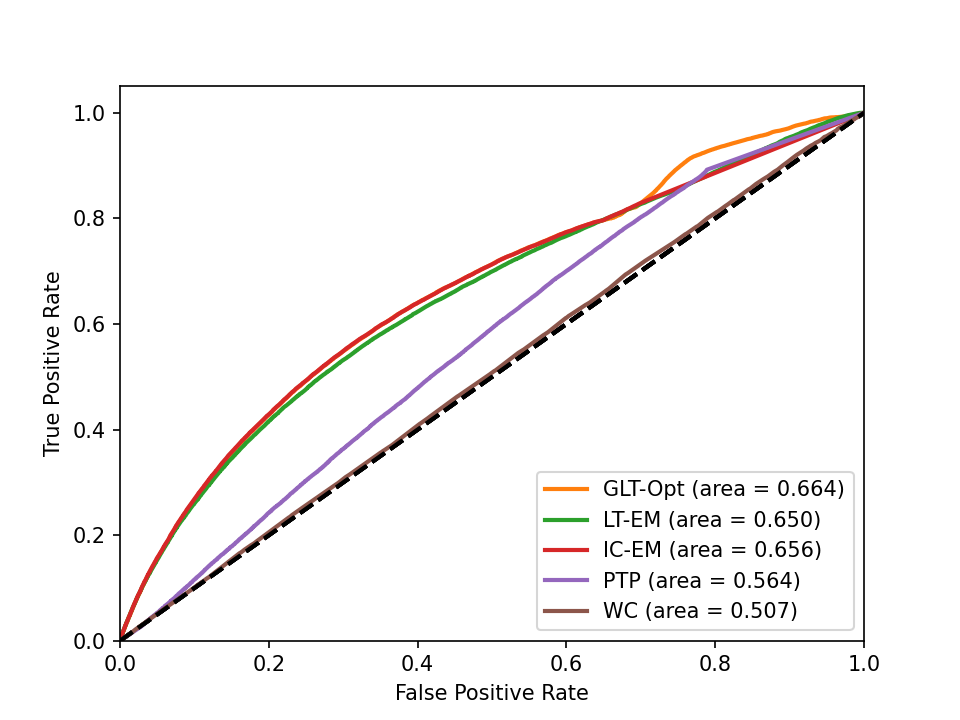
For each node , we extract pseudo-traces where was activated () by identifying all actions it performed and noting the set of ’s parents who performed before . For pseudo-traces where was not activated (), we consider all actions that did not perform but at least one of its parents did, noting the set of all its active parents at the last recorded time point in the action log. In such a way, we construct the pseudo-trace collection for each node in the graph. We then randomly split the data into training and test sets in a 4:1 ratio, stratified by the activation status . Using the same candidate diffusion models as in Section 5.2, we estimate the models based on the training pseudo-traces and compute the predicted node activation probabilities on the test pseudo-traces. The only difference is that when fitting the GLT model, we use a larger parameter grid for the Beta threshold distribution:
Note that for the fitting problem (21), we only require to be log-concave, which is satisfied when both and are greater than or equal to 1 for the Beta distribution. This differs from solving the IM problem under the estimated model, which would require to be concave, as indicated by Corollary 3.1. Figure 8 presents the resulting ROC curves and AUC scores for the estimated diffusion models. To check the robustness of these results to the choice of the training-test split, we repeat the process five times with different random seeds. The obtained AUC scores differ from those in Figure 8 by less than 0.001, so we do not report them here. The results show that GLT-Opt has a slight advantage over LT-EM and IC-EM, while all three models significantly outperform the heuristics PTP and WC.
6 Discussion
In this paper, we have proposed the general linear threshold (GLT) model for information diffusion on networks, derived identifiability conditions for edge weights, developed a likelihood-based method to estimate them from fully or partially observed traces, and proved that these estimates are consistent. An important assumption needed for consistency is the compactness of the parameter space, which prevents us from using threshold distributions with unbounded support, such as the exponential distributions. While consistency could likely still be established in these cases using standard parameter space compactification techniques, we found empirically that MLE solutions obtained by solving problem (16) are not always stable for such distributions (experiments are not included in the paper but are available on GitHub). This is likely because there are some special cases, for example, if for an edge we observe only traces where is activated immediately after or not at all, the weight estimate diverges. We leave the investigation of threshold distributions with unbounded support for future work.
To allow for easy use with arbitrary distribution of thresholds, our implementation of the likelihood optimization problem (16) uses the SLSQP solver, which accommodates both convex and non-convex problems. This choice was made to allow for fitting the GLT model with non-log-concave threshold densities, which may violate the convexity condition in Proposition 4.3. When convexity is guaranteed, however, optimization efficiency can be significantly improved by using convex solvers, such as Gurobi (Gurobi Optimization, LLC, 2024) or Mosek (ApS, 2019). Incorporating alternative solver options will be incorporated in future work.
In (21), we used a grid search to estimate the parameters of threshold distributions. While this approach is reasonable for distributions with a small number of parameters, it does not scale well. A possible alternative is nonparametric estimation, as discussed at the end of Section 4.5.
Another extension we leave for future work is establishing identifiability and consistency conditions for the GLT model where both the parent edge weights and the threshold distribution parameters vary with . We should still be able to estimate the parameters of the nodes that appear in a sufficient number of traces, but additionally allowing for threshold parameters would reduce the effective sample size, and limit the usefulness of the method to applications with a larger number of traces available.
Finally, it should be straightforward to establish asymptotic normality of the MLE for both the IC and the GLT models with appropriate regularity conditions on the weight distribution. That could be used to conduct inference, constructing confidence intervals or hypothesis tests, for example, to compare influence of parent nodes on a particular user, though we did not pursue this direction as it is rarely the purpose of information spread modeling.
References
- ApS [2019] MOSEK ApS. The MOSEK optimization toolbox for MATLAB manual. Version 9.0., 2019. URL http://docs.mosek.com/9.0/toolbox/index.html.
- Banerjee et al. [2020] Suman Banerjee, Mamata Jenamani, and Dilip Kumar Pratihar. A survey on influence maximization in a social network. Knowledge and Information Systems, 62:3417–3455, 2020.
- Cornuéjols et al. [1977] Gérard Cornuéjols, Marshall Fisher, and George Nemhauser. Location of bank accounts to optimize float: An analytic study of exact and approximate algorithms. Management Science, 23:789–810, 04 1977. doi: 10.1287/mnsc.23.8.789.
- Dinh and Parulian [2020] Ly Dinh and Nikolaus Nova Parulian. Covid-19 pandemic and information diffusion analysis on twitter. Proceedings of the Association for Information Science and Technology. Association for Information Science and Technology, 57, 2020.
- Erdös and Rényi [1959] P. Erdös and A. Rényi. On random graphs i. Publicationes Mathematicae Debrecen, 6:290, 1959.
- Farnad et al. [2020] Golnoosh Farnad, Behrouz Babaki, and Michel Gendreau. A unifying framework for fairness-aware influence maximization. In Companion Proceedings of the Web Conference 2020, WWW ’20, page 714–722, New York, NY, USA, 2020. Association for Computing Machinery. ISBN 9781450370240. doi: 10.1145/3366424.3383555. URL https://doi.org/10.1145/3366424.3383555.
- Gkioulekas [2013] Eleftherios Gkioulekas. On equivalent characterizations of convexity of functions. International Journal of Mathematical Education in Science and Technology, 44(3):410–417, 2013. doi: 10.1080/0020739X.2012.703336. URL https://doi.org/10.1080/0020739X.2012.703336.
- Goldenberg et al. [2001] Jacob Goldenberg, Barak Libai, and Eitan Muller. Talk of the network: A complex systems look at the underlying process of word-of-mouth. Marketing Letters, 2001.
- Goyal et al. [2011] Amit Goyal, Francesco Bonchi, and Laks V. S. Lakshmanan. A data-based approach to social influence maximization. Proc. VLDB Endow., 5(1):73–84, sep 2011. ISSN 2150-8097. doi: 10.14778/2047485.2047492. URL https://doi.org/10.14778/2047485.2047492.
- Granovetter [1978] Mark Granovetter. Threshold models of collective behavior. American journal of sociology, 83(6):1420–1443, 1978.
- Gurobi Optimization, LLC [2024] Gurobi Optimization, LLC. Gurobi Optimizer Reference Manual, 2024. URL https://www.gurobi.com.
- He et al. [2016] Xinran He, Ke Xu, David Kempe, and Yan Liu. Learning influence functions from incomplete observations, 2016. URL https://arxiv.org/abs/1611.02305.
- Jensen [1906] J. L. W. V. Jensen. Sur les fonctions convexes et les inégalités entre les valeurs moyennes. Acta Mathematica, 30:175–193, 1906. URL https://api.semanticscholar.org/CorpusID:120669169.
- Jones et al. [2001] Eric Jones, Travis Oliphant, Pearu Peterson, et al. SciPy: Open source scientific tools for Python, 2001. URL http://www.scipy.org/.
- Keener [2010] R.W. Keener. Theoretical statistics: Topics for a core course. 2010. URL https://books.google.co.in/books?id=aVJmcega44cC.
- Kempe et al. [2003] David Kempe, Jon Kleinberg, and Éva Tardos. Maximizing the spread of influence through a social network. page 137–146, 2003. doi: 10.1145/956750.956769. URL https://doi.org/10.1145/956750.956769.
- Kojaku and Masuda [2018] Sadamori Kojaku and Naoki Masuda. Core-periphery structure requires something else in the network. New Journal of Physics, 20(4):043012, apr 2018. doi: 10.1088/1367-2630/aab547. URL https://dx.doi.org/10.1088/1367-2630/aab547.
- Lancichinetti and Fortunato [2009] Andrea Lancichinetti and Santo Fortunato. Community detection algorithms: A comparative analysis. Physical Review E, 80(5), nov 2009. doi: 10.1103/physreve.80.056117. URL https://doi.org/10.1103%2Fphysreve.80.056117.
- Liu and Wu [2018] Yang Liu and Yi-Fang Brook Wu. Early detection of fake news on social media through propagation path classification with recurrent and convolutional networks. In Proceedings of the Thirty-Second AAAI Conference on Artificial Intelligence and Thirtieth Innovative Applications of Artificial Intelligence Conference and Eighth AAAI Symposium on Educational Advances in Artificial Intelligence, AAAI’18/IAAI’18/EAAI’18. AAAI Press, 2018. ISBN 978-1-57735-800-8.
- Mossel and Roch [2010] Elchanan Mossel and Sebastien Roch. Submodularity of infuence in social networks: From local to global. SIAM Journal on Computing, 39:2176–2188, 03 2010. doi: 10.1137/080714452.
- Narasimhan et al. [2015] Harikrishna Narasimhan, David C Parkes, and Yaron Singer. Learnability of influence in networks. In C. Cortes, N. Lawrence, D. Lee, M. Sugiyama, and R. Garnett, editors, Advances in Neural Information Processing Systems, volume 28. Curran Associates, Inc., 2015. URL https://proceedings.neurips.cc/paper_files/paper/2015/file/4a2ddf148c5a9c42151a529e8cbdcc06-Paper.pdf.
- Nemhauser et al. [1978] George Nemhauser, Laurence Wolsey, and M. Fisher. An analysis of approximations for maximizing submodular set functions—i. Mathematical Programming, 14:265–294, 12 1978. doi: 10.1007/BF01588971.
- Prékopa [1973] András Prékopa. On logarithmic concave measures and functions. 1973.
- Richardson and Domingos [2002] Matthew Richardson and Pedro Domingos. Mining knowledge-sharing sites for viral marketing. In Proceedings of the Eighth ACM SIGKDD International Conference on Knowledge Discovery and Data Mining, KDD ’02, page 61–70, New York, NY, USA, 2002. Association for Computing Machinery. ISBN 158113567X. doi: 10.1145/775047.775057. URL https://doi.org/10.1145/775047.775057.
- Rodriguez et al. [2014] Manuel Rodriguez, Jure Leskovec, David Balduzzi, and Bernhard Schölkopf. Uncovering the structure and temporal dynamics of information propagation. Network Science, 2:26–65, 04 2014. doi: 10.1017/nws.2014.3.
- Saito et al. [2008] Kazumi Saito, Ryohei Nakano, and Masahiro Kimura. Prediction of information diffusion probabilities for independent cascade model. KES ’08, page 67–75, Berlin, Heidelberg, 2008. Springer-Verlag. ISBN 9783540855668. doi: 10.1007/978-3-540-85567-5_9. URL https://doi.org/10.1007/978-3-540-85567-5_9.
- Tantardini et al. [2019] Mattia Tantardini, Francesca Ieva, Lucia Tajoli, and Carlo Piccardi. Comparing methods for comparing networks. Scientific Reports, 9, 11 2019. doi: 10.1038/s41598-019-53708-y.
- Turnbull [1976] Bruce W. Turnbull. The empirical distribution function with arbitrarily grouped, censored, and truncated data. Journal of the royal statistical society series b-methodological, 38:290–295, 1976. URL https://api.semanticscholar.org/CorpusID:122426592.
7 Appendix
A Proofs
A.1 Proof of Proposition 4.3
Let be an arbitrary cumulative distribution function with density . We need to show that
| (32) |
is concave on . Notice that is a log-concave function since for any and points with , it holds:
Thus, the expression under the integral in (32) is log-concave as a product of log-concave functions. Finally, by Theorem 6 in Prékopa [1973], the integral of a multivariate log-concave function w.r.t. any of its arguments is also log-concave. This completes the proof.
A.2 Proof of Proposition 3.2
Consider a GLT model on the directed graph with nodes and edges having equal weights . Let also node have a threshold cdf satisfying
An example of such can be constructed using Lagrange interpolation:
Notice that due to Theorem 3.2, the influence function of this GLT model is submodular since is concave on :
and threshold distributions of nodes 1, 2, and 3 do not affect the diffusion model as other nodes cannot activate them. Due to the same reason, the Triggering model on this graph will have only 8 parameters representing probabilities of node to choose each possible subset of as its triggering set. We will denote this probability distribution as
If the GLT model was a special case of the Triggering model, we could find an appropriate distribution such that the activation probability of node 4 is the same for the two models given any seed set, i.e. the following linear system should hold:
Solving this system we obtain:
But expanding the last row of the matrix we obtain that probability is a negative number. Contradiction.
A.3 Proof of Theorem 3.2
We start with the following technical lemma:
Lemma 7.1.
Consider cdf of the distribution supported on . Then the condition
| (33) |
holds for all triples with if and only if is concave on .
Proof of Lemma 7.1.
(Necessity) It is enough to verify the “midpoint” concavity condition:
since for bounded functions (cdf is bounded between 0 and 1), it is equivalent to concavity (see Section 5 of Jensen [1906]).
Plugging into (33) and rearranging the terms implies the needed inequality.
(Sufficiency) First notice that WLOG we can assume that . Indeed, if we can make a substitution and rearrange the terms in the target inequality to obtain:
where clearly . Now we are left to demonstrate that for and concave cdf , it holds:
This, in turn, follows from the equivalent definition of a concave function (Lemma 2.1 in Gkioulekas [2013]) which states that for any it should hold:
Indeed, applying this inequality to and we deduce what was needed:
The proof is complete. ∎
Proof of Theorem 3.2.
Consider a graph and an arbitrary GLT model on it. By Theorem 3.1, it is enough to show that all threshold functions are monotone and submodular. Monotonicity holds trivially since all edge weights are nonnegative and is non-decreasing. To establish submodularity, we need to check for and that
This follows by applying Lemma 7.1 to . The condition follows from weights’ non-negativity:
∎
A.4 Proof of Theorem 4.1
(Sufficiency) Assume there are distinct vectors of parameters and in for which . Since , there is an edge such that . Define the vectors of ’s parent edges as
For a subset , we will also denote
Consider the subsets of together with corresponding traces satisfying conditions of the theorem. Notice that equality of distributions and implies equality of diffusion models by (1), thus
| (34) |
Notice that here we used the fact that since otherwise both probabilities would be zero. In case , i.e. if , the negative term becomes zero on both sides due to . Thus, by invertibility of we deduce . But the set of ’s parents lying in is exactly , thus:
| (35) |
In case , the trace becomes also feasible by Lemma 4.1. Therefore, we have:
Summing this equality with (34) and inverting implies that both and should hold. But the difference between the two equations again gives (35) since
Combining (35) across all , we obtain a linear system which in matrix form can be written as
But according to our assumption, is invertible, thus and in particular. Contradiction.
(Necessity) Assume is identifiable but there is with for which conditions of the theorem do not hold.
Take arbitrary such that (it is in since ).
Our further goal is to obtain a contradiction by constructing coinciding with everywhere except for so that . Consider all possible subsets which satisfy condition 1 of the theorem. Then, our assumption implies that the matrix has . In other words, there is a non-zero vector such that . Thus, for any scalar , we can define to make it different from while preserving
| (36) |
We pick so that . Indeed, by triangular inequality, satisfies all the needed constraints:
Notice that by changing alone, we could only change the probability of a feasible trace with and for some where is the last time is not activated. Indeed, if then and if for any , then by (4), trace probability does not depend on . Take arbitrary such trace and consider all times for which . Notice that for each time the trace is also feasible and satisfies condition 1 of the theorem. Therefore, there is a corresponding column in matrix which according to (36) satisfies:
Summing these equations over and , we obtain respectively:
But from (4), trace probability is either a function of if or of and if . Therefore, we deduce and finally get the contradiction with identifiability of .
A.5 Identifiability and consistency for pseudo-traces.
(Proof of Theorem 4.3.
) It is enough to check that for , condition 1 in this theorem and Theorem 4.1 are equivalent. First, consider a subset with . Then clearly the trace that stopped at the seed set without propagating further satisfies condition 1 of Theorem 4.1. Now, assume there is a trace with , , and . Notice that given a seed set , the only feasible traces on we can get are either or . But , thus and . The proof is complete. ∎
A.6 Identifiability and consistency under the IC model.
By Definition 5, the likelihood of a feasible trace sampled from the IC model with edge probabilities and the seed distribution can be written as
| (37) |
Similarly to Assumption 2, we will assume that the ground-truth probabilities are separated from zero and one for identifiability:
Assumption 3.
There is a universal constant such that the true edge probabilities satisfy for all .
Then, for the truncated parameter space
| (38) |
we can formulate the same identifiability condition as for the GLT model:
Theorem 7.1.
Parametric family is identifiable if and only if for each child node with , there exist such that
-
1.
For each , there is a feasible trace with , , and .
-
2.
The matrix is invertible.
Proof.
(Sufficiency) Assume there are distinct vectors of parameters and in for which . Since , there is an edge such that . Define the vectors of ’s parent edge probabilities
as well as vectors
For a subset , we will also denote
Consider the subsets of together with corresponding traces satisfying conditions of the theorem. Notice that equality of distributions and implies equality of diffusion models by (1), thus
Notice that here we used the fact that since otherwise both probabilities would be zero. But by definition of , we have , therefore subtracting one and taking logarithm from both sides implies
Combining these equations across all , we obtain a linear system which in matrix form can be written as .
But according to our assumption, is invertible, thus . Element-wise exponentiation implies . Contradiction.
(Necessity) Assume is identifiable but there is with for which conditions of the theorem do not hold.
Take arbitrary such that (it is in since ).
Our further goal is to obtain a contradiction by constructing coinciding with everywhere except for so that . Consider all possible subsets which satisfy condition 1 of the theorem. Then, our assumption implies that the matrix has . In other words, there is a non-zero vector such that . Thus, for any scalar , we can define to make it different from while preserving
| (39) |
We pick so that satisfies the parameter space constraints:
Notice that by changing alone, we could only change the probability of a feasible trace with and for some where is the last time is not activated. Indeed, if then and if for any , then by (37), trace probability does not depend on . Take arbitrary such trace and consider all times for which . Notice that for each time the trace is also feasible and satisfies condition 1 of the theorem. Therefore, there is a corresponding column in matrix which according to (39) satisfies:
Summing these equations over and , we obtain respectively:
But from (37), trace probability is either a function of if or of and if . Therefore, we deduce and finally get the contradiction with identifiability of . ∎
Now, assume that as in (11), we observe a collection of independent traces sampled from the IC model, by which we mean that are independently sampled from and the edge activation random variables
are also independent across traces. Then, we can estimate by solving
| (40) |
where the log-likelihood of the trace , by (37), takes the form:
| (41) |
Notice that problem (40) is non-convex which motivated Saito et al. [2008] to use the EM-algorithm for estimating the IC model parameters. However, we still can state the following consistency theorem for the global optimum of problem (40):
Theorem 7.2.
B Additional Experiments
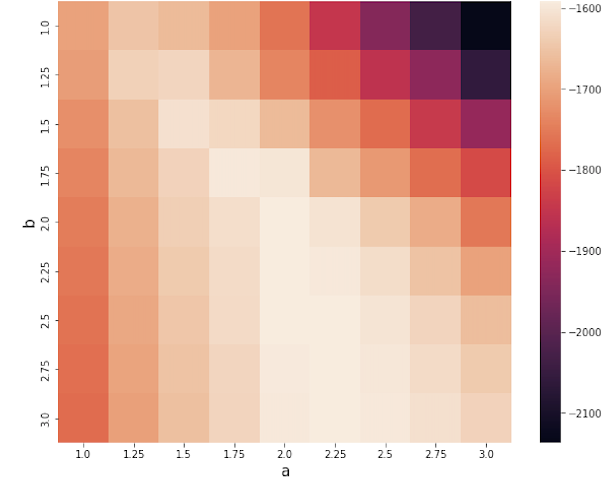
B.1 Grid Search for Beta distribution
Let be a -node graph generated from the directed version of the ER model [Erdös and Rényi, 1959] with . For this graph, consider an instance of the GLT model with for all nodes and weights generated as in (27). From this GLT model, we generate 2500 traces and split them randomly into 2000 train and 500 test traces. Finally, for each pair of threshold parameters in the grid
we set all threshold distributions as , estimate the weights by solving (16) using the train traces, and compute the log-likelihood on the test set under . The following heatmap shows that the highest log-likelihood is achieved for the true . Moreover, relatively high log-likelihood values for pairs close to the line show that guessing the mean structure of the distribution () is already enough for accurate model estimation.
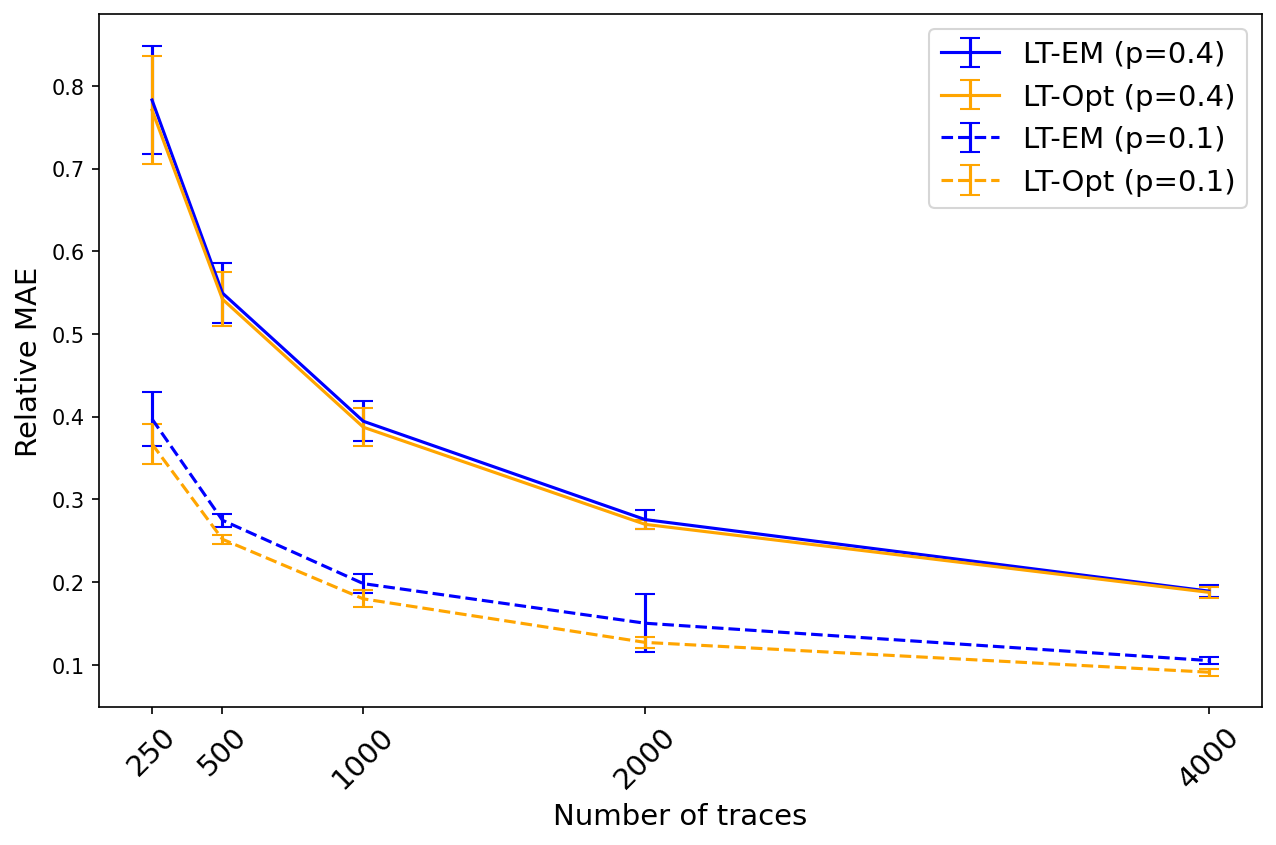
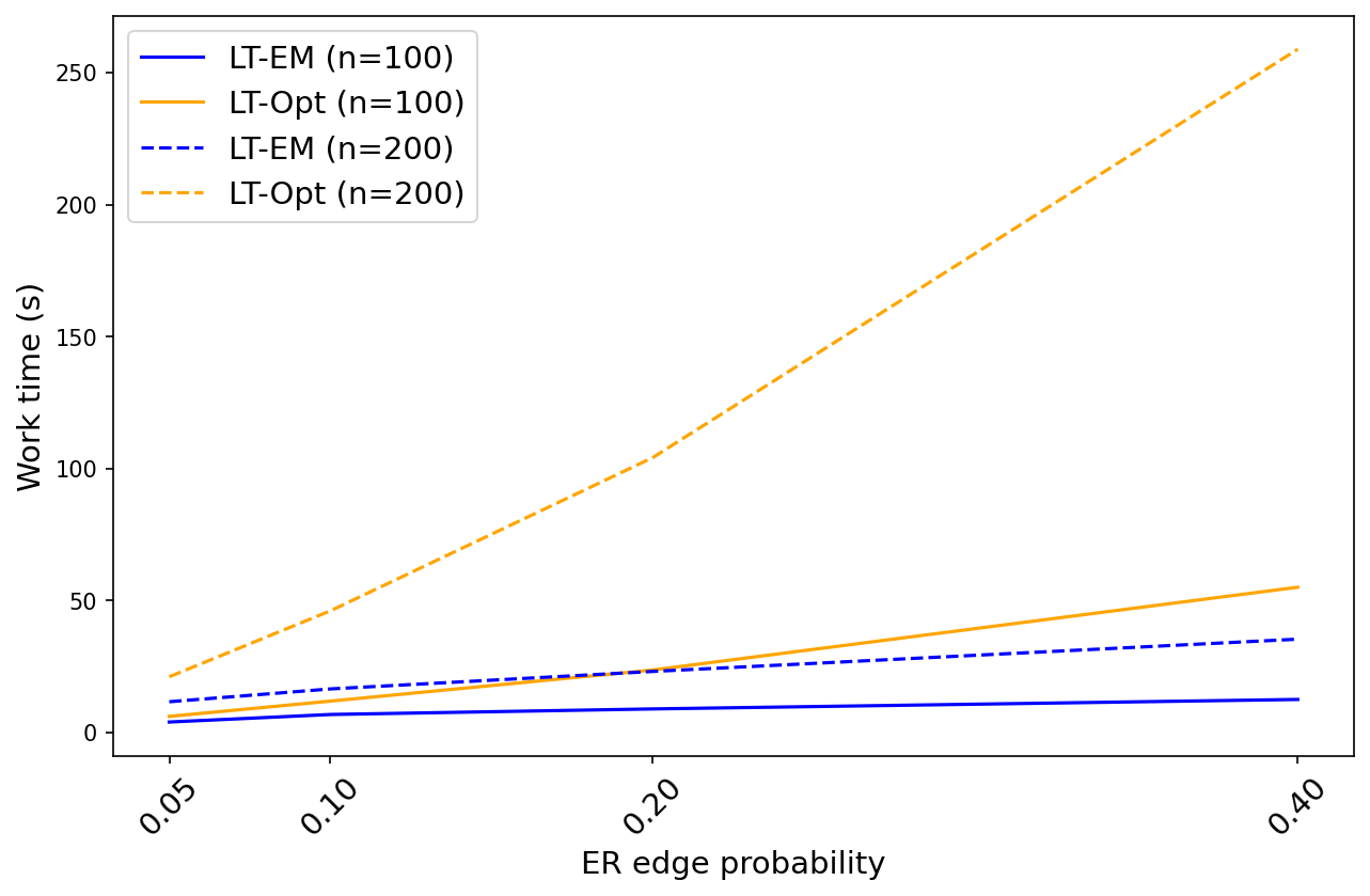
B.2 Estimation of the LT model using problem (16) vs Algorithm 2
To compare problem (16) (LT-Opt) and Algorithm 2 (LT-EM) in terms of the speed and accuracy of fitting the LT model, we conduct two experiments. In the first one, we generate two directed ER graphs with and . For each of them, we sample 4000 traces from the LT model with weights generated as in (27) and seed sets as in (26). Then for each trace set size , we fit the model with the first traces out of these 4000 and note the RMAE (defined in (29)) between the estimated and ground-truth weights. In the second experiment, we fix the number of train traces and for two sizes of the ER network , check how their density affects the run time of the estimation procedures. We change the density by varying the ER edge probability . The ground-truth LT model again has weights generated as in (27) and seed sets as in (26). Both experiments are run on 1 CPU to compare the methods in a scenario when no parallelization resources are available.
Results are presented in Figure 10. In the left plot, we can see that LT-Opt has a small edge in terms of the estimation accuracy which becomes less apparent with the increase of the network density (parameter ). On the other hand, the right plot demonstrates that with no parallelization resources at hand, the run time of LT-Opt is catastrophic compared to LT-EM, especially at higher values of the network density.