Set-Based Retrograde Analysis:
Precomputing the Solution to 24-card Bridge Double Dummy Deals

Abstract

Retrograde analysis is used in game-playing programs to solve states at the end of a game, working backwards toward the start of the game. The algorithm iterates through and computes the perfect-play value for as many states as resources allow. We introduce setrograde analysis which achieves the same results by operating on sets of states that have the same game value. The algorithm is demonstrated by computing exact solutions for Bridge double dummy card-play. For deals with 24 cards remaining to be played ($10^{27}$ states, which can be reduced to $10^{15}$ states using preexisting techniques), we strongly solve all deals. The setrograde algorithm performs a factor of $10^{3}$ fewer search operations than a standard retrograde algorithm, producing a database with a factor of $10^{4}$ fewer entries. For applicable domains, this allows retrograde searching to reach unprecedented search depths.

1 Introduction

Some of the early high-performance game-playing programs relied on retrograde analysis and endgame databases for strong play. The most notable example is Checkers, where 39 trillion endgame positions, all those with 10 or fewer pieces, were used as part of the Chinook program (Schaeffer et al. 1992), and for solving Checkers (Schaeffer et al. 2007). Endgame databases are also used widely in Chess programs (Chess 2024), as well as in many other games (e.g., for solving Awari (Romein and Bal 2003)).

Endgame databases are most effective in games where there are far fewer positions at the end of the game than elsewhere. As a result, they have not been applied in games that do not have this property. For instance, Sturtevant (2003) noted that in 3-player Chinese Checkers a winning arrangement of a single player’s pieces in the game has approximately $10^{23}$ possible permutations of the other player’s pieces, making it infeasible to store all the variations of even a single winning configuration. While in Chinese Checkers each player has a unique endgame configuration (the other side’s piece locations are irrelevant), in Go the locations of both side’s pieces in a terminal state are important. Hence these games require significantly different analysis (Berlekamp and Wolfe 1994). In a 4-player trick-based card game such as Bridge, the last two tricks have $\binom{52}{2}\binom{50}{2}\binom{48}{2}\binom{46}{2}=1.9\times 10^{12}$ possible deals of the cards. However, there are only 16 ways for each deal to play out, meaning it is trivial to solve but storing all states (as done in Checkers) is difficult.

These numbers suggest it might be impractical to build an effective endgame database for Bridge with, say, 6 tricks to play ($10^{27}$ states). This statement is true under the assumption that every unique endgame state must be stored independently. The contribution of this paper is to show how to avoid this assumption by representing endgame states as sets. This idea, along with other symmetry reduction techniques, makes it feasible to use retrograde search to compute all 24-card (6-trick) Bridge double-dummy (DD) endgames in a week on appropriate hardware using just 50GiB of storage, something that was historically hard to imagine.

This paper describes our set-based approach to endgame databases, making the following contributions.

• We present a new set-based retrograde analysis algorithm, setrograde analysis, inspired by the ideas in Ginsberg’s Partition Search (Ginsberg 1996). Whereas standard retrograde analysis computes a value for every state, setrograde analysis generalizes a state into a set where all members have the same game-theoretic value. The algorithm can skip over many of the states that are subsumed by the set. Replacing states with sets leads to a large degree of state-space compression, by mapping an exponentially growing state-space to a smaller set-space.

• The algorithm is demonstrated using 24-card Bridge deals. The set database contains 4 orders of magnitude (OOM) fewer sets than there are states in a traditionally generated database. The set database was constructed using 3 OOM less computing resources than would be needed for a traditional 24-card database. This enabled an 800 trillion state state-space to be solved in a week using a single multi-core machine.

This work generalizes retrograde analysis, allowing it to have more impact in applicable domains. In particular, the reduced computing and storage needs mean that endgame database technology can be scaled to unprecedented levels.

2 Background and Related Work

Double-dummy problems are the perfect-information variant of Bridge card play. A deal of $n$ cards (with $n$ as a multiple of 4) has an exact integer evaluation under perfect play, ranging from 0 to $\frac{n}{4}$ — the number of tricks won. See Fig. 1 (left) for a one-suit, two-card deal; the four player around the table are referred to as North, South, East and West.

The idea behind retrograde analysis is to solve a game from the end towards the start. In the example of Bridge, this works by enumerating all deals where each player has one card (1 trick), solving them, and then storing the results. Then one can move backwards in the game to consider all deals where each player has two cards (2 tricks). For a given 2-trick deal, taking the maximum result of all successor 1-trick deals (already computed) produces the correct result. Given sufficient computational and storage resources, one could continue to obtain the 3-trick results, and so on. Most often the algorithm is expressed as solving depth $d$ (where $d$ is the number of tricks in Bridge or the number of pieces on the board as in Chess) given the precomputed results from depth $d-1$. The computational cost and storage requirements typically grow exponentially in $d$. There are numerous enhancements to the basic algorithm that can improve its performance (Sturtevant and Saffidine 2017). Retrograde analysis is typically used to compute and store the value for all states up to a given depth $d$, producing a comprehensive database (often called an endgame database or tablebase).

Since evaluations are discrete, $n$-card deals may be grouped into consistent sets, meaning that all states in the set share the same evaluation. Partition Search (Ginsberg 1996) is a forward minimax solver with a set-based backup heuristic that generates a consistent set at each state in the search. Ginsberg showed a branching factor reduction by using these sets as transposition table entries. DD solvers based on Partition Search remain a state-of-the-art tool for modern mechanical Bridge players.

Bridge deals are colloquially described by the number of cards in each suit, and the ranks of relevant high cards. A sufficiently low card, that does not affect the result, is usually referred to as x. This notion is formalized in the set representation we use. Any card denoted x is interchangeable with any other x, and is strictly lower than a ranked card. For example, Fig. 1 (right) shows a set containing $6!/(2!)^{3}=90$ states that Partition Search might discover by generalizing the state in Fig. 1 (left).

Partition Search maintains consistent sets by heuristically backing up cards that can be proven to never win by rank. Available DD solvers rely on expert heuristics for move ordering, set generation, and early search cutoffs. For retrograde searching, we present a more general algorithm for proving consistent sets and a framework in which the need for expert knowledge is eliminated.

	N			$\spadesuit$98		$\spadesuit$98
W		E	$\spadesuit$54		$\spadesuit$32 $\rightarrow$ $\spadesuit$xx		$\spadesuit$xx
	S			$\spadesuit$76		$\spadesuit$xx

Figure 1: $\spadesuit$98 wins two tricks regardless of the locations of lower cards in the perfect-information deal (left) and set of deals (right); x refers to any low card. Play proceeds clockwise starting with North (N) until each player has played one card (East, South, West). The highest card wins. The winning player is next-to-play.

There have been previous attempts at set-based search algorithms in games, but they bear little resemblance to our approach and they have not been applied (or are even relevant) to backward search. Our algorithms are designed to strongly solve large state-spaces (finding the perfect play result for all reachable states) using retrograde analysis. Previous approaches have aimed at weakly solving state-spaces using a top-down approach. Retrograde state-space search has seen success in board games including Checkers (Schaeffer et al. 2007), Chinese Checkers (Sturtevant 2020), and Chess (Chess 2024). Retrograde analysis has been applied to a subset of Skat (null) endgames (Furtak 2013). All of the set-wise approaches that we know of, including Proof-Set Search (Müller 2002), Method of Analogies (Adelson-Velsky, Arlazarov, and Donskoy 1988), and even Partition Search (Ginsberg 1996), have been designed for top-down search, and targeted toward weak solutions (Haglund and Hein 2014; Beling 2017). Set-based search has been applied successfully in planning, where sets of states are often represented using Binary Decision Diagrams (Edelkamp, Kissmann, and Torralba 2015).

3 Overview

Here we provide a high-level overview of a set-based approach to retrograde analysis. The ideas are illustrated using examples from Bridge.

3.1 State-Space Reduction

This section is specific to the game of Bridge, but is important for illustrating the search-space reductions that are possible in Bridge and in set-based search.

A 24-card (6 tricks) endgame database contains the solution to all ${52\choose 6}{46\choose 6}{40\choose 6}{34\choose 6}=10^{27}$ ways to distribute the cards from a standard deck. Additionally, there are 5 trump suits to consider (clubs, diamonds, hearts, spades, and no trump). Hence there are $5\times 10^{27}$ unique deals represented in the 24-card database.

A well-known optimization used in card-game transposition tables is to represent cards using relative ranks instead of absolute ranks (Haglund and Hein 2014). If there are 8 spade cards in play, the lowest one is always represented as a 2, the next lowest as a 3, and so on. Thus, $13\choose 8$ possible deals (1,287) are reduced to 1 representative deal. This does not affect card-play mechanics, but it reduces the number of 24-card states by roughly 12 OOM. Several minor symmetry-related optimizations (not discussed here) can be applied to remove approximately one OOM, leaving $8\times 10^{14}$ (800 trillion) distinct states that must be evaluated and stored in a 24-card endgame database.

Table 1 provides the number of states given the number of cards remaining. Upper Bound is the number of states a state-based retrograde solver would need to both solve and store (after the rank and symmetry state-space reductions). Setrograde is the number of sets stored in our set-based database through 24 cards. At the time of this writing, the 28 card results are being computed. Lower Bound is a bound on the number of sets in a complete DD database, assuming an approach that partitions the state-space by the distribution of suits between the players. The data in this table is discussed in more depth later in the paper.

Table 1 demonstrates two major state-space reductions, and their scaling. As the number of cards increases, the relative-rank state-space reduction increases rapidly at first, peaking with a 12 OOM reduction at 24 and 28 cards. Beyond 28 cards, this reduction decreases with depth. Once 52 cards remain, all 13 cards in each suit are represented at all times, and no rank reduction exists. (The reduction that remains is due to symmetries.) The size of the set-space considered by the setrograde analysis algorithm (introduced in this paper) are also shown. Set-space growth seems to be decelerating (e.g., growing by almost 2 OOM going from 16 to 20 cards, but only 1 OOM in going from 20 to 24), and grows much more slowly than the state-space. As the number of cards increase, larger sets are produced.

Cards	States	Upper Bound	Setrograde	Lower Bound
4	$3\times 10^{7}$	$2\times 10^{2}$	$7\times 10^{1}$	$2\times 10^{1}$
8	$9\times 10^{12}$	$8\times 10^{4}$	$8\times 10^{3}$	$5\times 10^{2}$
12	$4\times 10^{17}$	$3\times 10^{7}$	$5\times 10^{5}$	$7\times 10^{3}$
16	$3\times 10^{21}$	$1\times 10^{10}$	$3\times 10^{7}$	$6\times 10^{4}$
20	$7\times 10^{24}$	$3\times 10^{12}$	$1\times 10^{9}$	$4\times 10^{5}$
24	$5\times 10^{27}$	$8\times 10^{14}$	$2\times 10^{10}$	$2\times 10^{6}$
28	$1\times 10^{30}$	$2\times 10^{17}$	-	$7\times 10^{6}$
32	$6\times 10^{31}$	$3\times 10^{19}$	-	$2\times 10^{7}$
36	$1\times 10^{33}$	$4\times 10^{21}$	-	$4\times 10^{7}$
40	$5\times 10^{33}$	$4\times 10^{23}$	-	$4\times 10^{7}$
44	$4\times 10^{33}$	$4\times 10^{25}$	-	$3\times 10^{7}$
48	$3\times 10^{32}$	$2\times 10^{27}$	-	$9\times 10^{6}$
52	$3\times 10^{29}$	$1\times 10^{28}$	-	$2\times 10^{6}$

Table 1: State-Space Size and Reductions for Bridge

3.2 Set-Space Reduction

Retrograde analysis, shown in Alg. 1, works by iterating over all states at depth $d$ (lines 3-4, 12-13), computing a state’s value based on the successor states at depth $d-1$ (line 5), and storing it into the database (line 7). Applying the same approach to 24-card Bridge would require repeatedly iterating over almost $10^{15}$ states (assuming the reductions given above), requiring storage of $\sim 10^{15}$ bytes (depending on possible compression approaches).

Our set-based algorithm, setrograde analysis, generates a database of consistent sets. We start with a simpler version of the algorithm, also shown in Alg 1, before refining our description into a more efficient version. As with retrograde analysis, the simpler implementation works by iterating through all states at depth $d$ (lines 3-4, 12-13). Each state is queried in the database to see if it matches any of the sets that have already been computed (line 5). If such a set is found, the state’s value is known and the algorithm moves on to the next state. Otherwise, a search routine finds a consistent set containing the new state (line 9), and that set is added to the database (line 10).

We highlight here some of the challenges in creating a fast setrograde algorithm:

1. Generalization. This additional routine (line 9) is performed at every state. The cost of this operation must be less than the cost of performing the retrograde operation for each of the states encompassed by the set returned.

2. Querying. It is more complex to look for a state in a database of sets than to look for a state in a database of states (line 5). $databaseLookup$ performs multiple queries at each state. Without a fast and scalable implementation, queries become a computational bottleneck.

3. Iteration. Iterating over all members of a large state-space will be expensive even if the cost per state is small. To scale computation, we must be able to iterate through the set-space without considering each state in the (much larger) state-space.

Algorithm 1 Retro/Setrograde Analysis

1:  for $d\leftarrow 1..D$ do

2:     $EDB_{d}\leftarrow\emptyset$

3:     $s\leftarrow\textit{firstState}(d)$

4:     while  $s\neq null$ do

5:        $v\leftarrow databaseLookup(s,d)$

6:        if $\textit{algorithm}=\textit{retroGrade}$ then

7:           $EDB_{d}[s]\leftarrow v$

8:        else if $EDB_{d}[s]=undefined$ then

9:           $t\leftarrow\textit{generalizeToSet}(s,v)$

10:           $EDB_{d}[t]\leftarrow v$

11:        end if

12:        $s\leftarrow nextState(s,d)$

13:     end while

14:  end for

Each of these are briefly described. Generalization and iteration are then illustrated using Bridge.

Generalization

In retrograde analysis, if a state is reached that is not in the database, then it will have its value computed and added to the database. Instead, setrograde analysis finds a generalization of the state (a set) in which all states have the same value (consistent). It does this using a generate-and-test approach, where sets are generated until the best consistent set (along some metric) is found. In Bridge, this is done by replacing some cards with x’s.

Generalization is illustrated in Bridge in Section 3.3. If all possible ways of generalizing a state are considered, this function would be very expensive. In the Technical Appendix, we show how the cost can be reduced by considering only a subset of generalizations.

Querying

In retrograde analysis, a ranking or perfect hash function is used to map every state to a unique number. States are not explicitly stored; the offset in memory uniquely identifies a state. In setrograde analysis, sets must be explicitly stored. Thus, looking up a state in the database (line 5) involves matching a state to a set, a more complicated operation. Querying can be done efficiently using an appropriate data structure. One such data structure is briefly discussed in the Technical Appendix.

Iteration

Some states can be bypassed, given that they are members of sets already in the database. Similar to how backjumping is used in DPLL search (Gaschnig 1979) to avoid searching irrelevant portions of a tree, it is possible to identify portions of the space that have already been solved, and jump past them. The exact approach is dependent on the state representation being used. Low-cost iteration is illustrated in Bridge in Section 3.4.

3.3 Example 1: Generalization in Bridge

In the following deal, East is on lead. North and South will take 2 tricks with the two highest spades:

	$\spadesuit$98					N
$\spadesuit$32		$\spadesuit$54			W		E
	$\spadesuit$76					S

a)	$\spadesuit$98		b)	$\spadesuit$98		c)	$\spadesuit$98
$\spadesuit$3x		$\spadesuit$54	$\spadesuit$xx		$\spadesuit$54	$\spadesuit$xx		$\spadesuit$5x
	$\spadesuit$76			$\spadesuit$76			$\spadesuit$76
d)	$\spadesuit$98		e)	$\spadesuit$98		f)	$\spadesuit$98
$\spadesuit$xx		$\spadesuit$xx	$\spadesuit$xx		$\spadesuit$xx	$\spadesuit$xx		$\spadesuit$xx
	$\spadesuit$76			$\spadesuit$7x			$\spadesuit$xx
g)	$\spadesuit$9x		h)	$\spadesuit$xx			N
$\spadesuit$xx		$\spadesuit$xx	$\spadesuit$xx		$\spadesuit$xx	W		E
	$\spadesuit$xx			$\spadesuit$xx			S

Figure 2: Sets generated by replacing 0 or more low-rank cards with x’s. East is on the lead.

To generalize this deal we must produce candidate sets. Here we use the 8 candidates (a-h) shown in Fig. 2 that were generated by replacing one or more low-rank cards with x’s. It can quickly be verified that sets a-f contain only states in which North and South take 2 tricks. For example, consider verifying set f using minimax search. East, South, and West each have one legal move (play an x), after which North plays either the 9 or the 8, winning the trick. The resultant set using relative card ranks is:

⬇ $\spadesuit$4 $\spadesuit$x $\spadesuit$x $\spadesuit$x

Having taken one trick, North and South must take one more trick in this resultant set. A search for this set in the 4-card database returns a value of one trick for North and South. Therefore this candidate set is a valid generalization. Note that in general, the exact set being looked for may not be in the database. Instead the overlap of several entries may be equivalent to the set looked for. The value of the overlapped sets would be the minimum of their values.

Sets g and h each contain at least one deal in which North and South take only one trick, for instance:

⬇ $\spadesuit$96 $\spadesuit$87 $\spadesuit$54 $\spadesuit$32

Consider trying to verify the correctness of g. Similar to the analysis of f above, East, South, and West again have one legal move and North has 2. North can play an x in which case North may fail to win the current trick. While a complex analysis can be performed when it is unclear which card wins a trick, it is sufficient here to note that in any case where North and South fail to win this trick, North and South will be unable to take 2 total tricks. Therefore, if North plays an x on best play, set g must not be consistent. North therefore plays the 9, producing the following resultant set:

⬇ $\spadesuit$x $\spadesuit$x $\spadesuit$x $\spadesuit$x

North and South must take one more trick in this resultant set. Searching the 4-card database finds the following entry, which overlaps the set being looked for. Here North and South take 0 more tricks:

⬇ $\spadesuit$x $\spadesuit$4 $\spadesuit$x $\spadesuit$x

This means on North’s action (the $\spadesuit$9) set g is not consistent. Since North has no legal actions that leads to consistent resultant positions, set g is not consistent and cannot be added to the database.

3.4 Example 2: Low-Cost Iteration in Bridge

To reduce computation, we skip over states that are members of the set just added to the database. We only solve and generalize independent states — states not yet represented in the database. Each time a set is added to the database, we generate one or more potential next-states. These states are constructed by applying minor changes to the previous set that give rise to states that are provably not represented by that set. The next states are placed into an open list (as in the A* algorithm (Hart, Nilsson, and Raphael 1968)) for further consideration. From the previous example, if we add to the database the set:

	$\spadesuit$98					N
$\spadesuit$xx		$\spadesuit$xx			W		E
	$\spadesuit$xx					S

it would be redundant to evaluate any other state in which North holds $\spadesuit 98$. Therefore an independent state can be produced efficiently by trading the $\spadesuit 8$ for one of the $\spadesuit$x cards. For example, we could produce the following set (one of three such possibilities):

⬇ $\spadesuit$9x $\spadesuit$xx $\spadesuit$xx $\spadesuit$8x

If this set is consistent then it will be turned into a state by replacing the x’s with low values (one of 720 possibilities):

⬇ $\spadesuit$97 $\spadesuit$32 $\spadesuit$54 $\spadesuit$86

This new state goes onto the open list and eventually gets generalized using the process shown in Example 1. This process repeats until all deals in the state-space are represented by a set in the database. Through this process, a setrograde solver can consider far fewer states than it would with the standard iteration over all states, reducing computation costs. Further insight into this process is included in the technical appendix.

4 Setrograde Analysis

Now we turn to a more complete description of setrograde analysis, identify further bottlenecks, and describe how these are implemented efficiently.

These definitions are used to describe setrograde analysis:

• $D$: maximum retrograde distance — in Bridge, number of tricks

• $d$: retrograde distance $d\in 1..D$ (that is, distance to terminal state)

• $\mathbf{S}_{d}$: all states at distance $d$ (from terminal state)

• $\mathbf{T}_{d}$: a set of sets of states such that all encapsulated states have a retrograde distance $d$

Algorithm 2 General Setrograde Analysis

1:  for $d\leftarrow 1..D$ do

2:     $\mathbf{T}_{d}\leftarrow\emptyset$

3:     $EDB_{d}\leftarrow\emptyset$

4:     $s\leftarrow\textit{nextIndependentState}(\mathbf{T}_{d})$

5:     while $s\neq$ null do

6:        $v\leftarrow\textit{databaseLookup}(s,d)$

7:        $t\leftarrow\textit{generalizeToSet}(s,v)$

8:        $\mathbf{T}_{d}\leftarrow\mathbf{T}_{d}\cup t$

9:        $EDB_{d}[t]\leftarrow v$

10:        $s\leftarrow\textit{nextIndependentState}(\mathbf{T}_{d})$

11:     end while

12:     compactEDB($EDB_{d}$)

13:  end for

Setrograde analysis (Alg. 2) parallels its state-wise predecessor with three key modifications. First, a set $\textbf{T}_{d}$ is maintained to track solved states (which are not stored explicitly but found in the union of all sets in $\textbf{T}_{d}$). Second, at each iteration, a state $s\in\mathbf{S}_{d}|s\notin\mathbf{T}_{d}$ is evaluated — that is, states that are already solved are not re-evaluated. While re-evaluation does not occur in the state-wise formulation, it could occur in the set-wise formulation if the states were evaluated iteratively without validating independence. Finally, each solved state is generalized to a consisistent set $t$. Set $t$ is stored in the database instead of the individual state.

Alg. 3 provides the helper functions needed for Alg. 2. The generalization process from a state to a consistent set can be done in many ways. One method is a backup heuristic, such as the one used in most modern Double Dummy solvers (Ginsberg 1996). The heuristic produces a single consistent set t. This approach opts for simplicity, ignoring generality at each step and incurring a compounding performance penalty in both computation and storage. For our setrograde solver, we use a generate-and-test approach. Multiple candidate sets are produced, which may or may not be consistent. Each is evaluated for consistency. Any metric (for instance $|\emph{}{t}|$) can be used to select which consistent set to add to the database.

Setrograde analysis is not guaranteed to produce the smallest possible database by any metric. The order in which states are evaluated can affect which sets are added to the database. The metric used to select which consistent candidate set is added to the database (or indeed whether multiple sets are added) can affect the composition of the final database. Some metrics (including $|\emph{t}|$) can result in ties, and the tiebreak can affect the composition and size of the database. Anything that affects the size of the database may also affect computation time since speed is positively correlated with the number of states that are evaluated and generalized. Future work might establish stronger performance guarantees or tighter bounds.

The lower bound on the number of sets required for a database is based on an ideal set representation in which all deals with the same game value are represented in a single set. In that case, we need exactly one set for each game value. In Bridge we partition the state-space based on the distribution of suits between the four hands. Since each partition requires at least one database entry (some partitions evaluate to a single game value), the number of partitions provides the tighter lower bound found in Table 1. This partitioning of both the state-space and set-space also makes our implementation embarrassingly parallelizable, as each partition can be solved independently.

5 Implementation in Bridge

This section briefly mentions some of the important Bridge implementation details. Further information can be found in the Technical Appendix.

Set Representation:

As discussed in the background section, and depicted in Fig. 1, representing sets of deals with low cards unspecified is not a new idea. This representation, with fixed cards and x’s is used in most (if not all) implementations of Partition Search. To reduce database size, we extend this methodology, by representing each card using four positional bits — one bit per player — indicating whether or not each player may hold this card. This representation allows for AND-OR conditions that are not possible with a simple $x$ notation for low cards. We demonstrate the utility of this representation by example.

In each of the four sets in Fig. 3 (top), North and South can take two tricks by playing the highest two cards, one on each trick. Since the evaluation of each set is identical (North and South take two tricks on perfect play), the union of the four sets is itself a consistent set. The union could be expressed as (North holds the $\spadesuit$9 OR South holds the $\spadesuit$9) AND (North holds the $\spadesuit$8 OR South holds the $\spadesuit$8) AND (all lower cards are x’s). Using 4 positional bits per-card (in North-South-East-West order) we can represent that statement compactly. The $\spadesuit$9 and $\spadesuit$8 each have their bits set to true (1) corresponding to North and South holding those cards, and two bits false (0) corresponding to East and West set not holding those cards, as illustrated in Fig. 3 (bottom). Our databases consist of entries mapping from sets represented in this syntax to a bound on the number of tricks taken by each partnership.

⬇ $\spadesuit$98 | $\spadesuit$xx $\spadesuit$xx $\spadesuit$xx | $\spadesuit$xx $\spadesuit$xx $\spadesuit$xx | $\spadesuit$98 ------------------------------- $\spadesuit$9x | $\spadesuit$8x $\spadesuit$xx $\spadesuit$xx | $\spadesuit$xx $\spadesuit$xx $\spadesuit$8x | $\spadesuit$9x

$\spadesuit$9	$\spadesuit$8	$\spadesuit$7	$\spadesuit$6	$\spadesuit$5	$\spadesuit$4	$\spadesuit$3	$\spadesuit$2
1100	1100	x	x	x	x	x	x

Figure 3: Top: $\spadesuit$98 wins two tricks regardless of the locations of lower cards in each set depicted. East is next-to-play in all diagrams. Bottom: Compact representation of the union of the sets above.

Low-Cost Generalization:

State generalization uses binary search. The lowest card in a suit can always be marked as $x$ and it is possible that entire suit (13 cards) could be $x$s. Hence for each suit a binary search is done on the number of $x$s. The program starts in the middle of the range and introduces that number of $x$s. Depending on whether the resulting set is consistent, the search either tries adding more or eliminating some $x$s. In some cases, the 4-bit representation used can compactly express the union of sets in the database, reducing database size. Compaction operations can be performed at insertion or in post-processing (Alg. 2, line 12).

Low-Cost Querying:

State lookups, matching a state to a set to retrieve a value, are achieved using a depth-limited tree data structure. At each node, a bitwise AND operation can be used to determine whether a state is in a set. The tree structure lets us minimize the nodes that need to be tested. Each node contains partial information, and if a node does not provide a partial match, its subtree can be pruned. The tree we use benefits from locality, and we maintain relatively small independent trees for each distribution of suits between players (Lower Bound in Table 1).

Disk Storage:

The 24-card database is partitioned into $10^{6}$ independent pieces (Lower Bound in Table 1), each one reflecting a different distribution of cards (the deal’s $shape$). Within each partition the sets are organized in a tree-like fashion. More details are in the Technical Appendix.

Algorithm 3 Setrograde Helper Functions

  # Returns value of a state.

  function databaseLookup(state $s$, distance $d$)

     return  $\max_{s^{\prime}\in\text{succ}(s)}EDB_{d-1}[s^{\prime}]$

  end

  

  # Returns a state that is not yet present in the EDB.

  function nextIndependentState(set of set of states $\mathbf{T_{d}}$)

     if $\exists s\in\mathbf{S}_{d}|s\notin\mathbf{T_{d}}$ then

        return  $s$

     end if

     return  null

  end

  

  # Returns whether all states in a set share given value.

  function ORACLE(set of states t, value v)

     return  $\not\exists s\in t|databaseLookup(s)\neq v$

  end

  

  # Returns a collection of candidate sets

  function generateCandidates(state s)

     return  $\{t\in 2^{\mathbf{S}_{d}}|s\in t\}$

  end

  

  # Returns a consistent set.

  function generalizeToSet(state s, value v)

     $t_{ret}\leftarrow s$

     $candidates\leftarrow generateCandidates(s)$

     while $\exists t_{c}\in candidatates\;s.t.|t_{c}|>|t_{ret}|$ do

        if $ORACLE(t_{c},v)$ then

           $t_{ret}\leftarrow t_{c}$

        end if

     end while

     return  $t_{ret}$

  end

6 Experimental Results

Here we provide an analysis of setrograde analysis performance on Bridge database generation. The program is written in Julia, and compiled in version 1.8 or higher using the LLVM compiler. All code is compatible with version 1.11. The large databases were computed on a machine with 48 cores, 187 GB of RAM, and 256 GB of swap using an Intel(R) Xeon(R) Gold 6248R CPU @ 3.00GHz.

6.1 Validation

Extensive tests to verify the correctness and completeness of our databases were performed. The simplest approach is to compute the retrograde analysis databases and then compare the results with the setrograde data. Retrograde databases were built through 16-card deals. Every state’s value in these databases was in agreement with the corresponding setrograde result.

Beyond 16 cards, exhaustive validation is no longer practical. We rely instead on two methods for partially validating the 20 and 24 databases. First, random subsets of the search space were chosen and for each state the setrograde value was compared to that of a standard minimax search. Second, thousands of double dummy problems were solved using a search-based solver with and without using the setrograde databases. The values returned in all the searches were identical.

Our results were validated to the extent that could reasonably be done on the available compute resources. Positive results have been achieved using every validation method we could practically implement.

6.2 Performance of Setrograde Analysis

Table 1 shows one measure of setrograde’s performance. Upper Bound is the number of states that a retrograde analysis program would considered (in the reduced search space). Setrograde is the number of sets that were needed to capture the exact same information. There is a $4\times 10^{4}$ reduction. This is slightly misleading as the cost to compute the value of a state is much less than the cost of producing a consistent set.

In Table 2 the storage and computational resources for retrograde and setrograde analysis are presented. Some of the retrograde numbers were too costly to run and their values are extrapolated (indicated by a †). The retrograde storage is pessimistic (two states per byte), given the potential for applying further data compression techniques. The computation times for retrograde are optimistic as they do not take into account performance loss due to scaling (e.g., loss of locality).

	DB Size (GiB)		Gen Time (CPU Days)		States/Byte
Cards	Retrograde	Setrograde	Retrograde	Setrograde	Setrograde
4	$1\times 10^{-7}$	$7\times 10^{-6}$	—	—	$2.6\times 10^{-2}$
8	$4\times 10^{-5}$	$3\times 10^{-5}$	—	—	$3.2\times 10^{0}$
12	$2\times 10^{-2}$	$1\times 10^{-3}$	$3\times 10^{-3}$	$1\times 10^{-4}$	$3.1\times 10^{1}$
16	†$5\times 10^{0}$	$5\times 10^{-2}$	$1\times 10^{0}$	$1\times 10^{-2}$	$1.9\times 10^{2}$
20	†$2\times 10^{3}$	$2\times 10^{0}$	†$4\times 10^{2}$	$2\times 10^{0}$	$1.6\times 10^{3}$
24	†$4\times 10^{5}$	$5\times 10^{1}$	†$1\times 10^{5}$	$3\times 10^{2}$	$1.5\times 10^{4}$

Table 2: Database Generation Time and Storage for Bridge

Database Size: The retrograde database sizes reported used $0.5$ bytes per state, indicating a deal’s value $0..d$. This representation reflects having a function that maps a state to a unique storage location with no gaps. Although we did not use such a function (it was too slow), the results are reported as if we did. Additional compression techniques (not done) could yield small gains. Retrograde database sizes scale linearly with the number of states in the state-space.

In contrast, setrograde has to store variable size sets (for 24 cards, ranging from 8 to 40 bytes, but compression gives a factor of 5 reduction). Despite the additional storage for a set, our setrograde database is almost 4 OOM smaller than its retrograde counterpart (before investigating data compression techniques for the retrograde counterpart).

Generation Time: The time taken to generate a database is presented in number of CPU days. Note that the machine used has 48 cores, meaning one day of wall-clock time corresponds to 48 CPU days.

Through 12 cards, the execution time for both retrograde and setrograde analysis are too small to draw meaningful conclusions. For the 16-card calculation, setrograde is completed with 2 OOM less time. The 20 and 24 card retrograde computations were not performed. Both retrograde and setrograde analysis are embarrassingly parallelizable for Bridge. The setrograde wall clock times for 20 and 24 cards were 1 hour, and 6 days respectively (on a 48 core machine).

States/Byte: The number of states divided by the size of the resulting database is a measure of information density. A retrograde solver would store roughly $2$ states per byte (somewhat higher with appropriate compression), regardless of the value of $d$. For setrograde the information density grows with $d$. Increasing $d$ means that a set, in general, reflects a larger number of states.

6.3 Breakdown of 24-card performance gains

Setrograde analysis decreases both storage and computation costs, rather than trading one for the other. To understand where the computation and storage costs are being reduced, we can break down the performance of setrograde analysis. In the 24-card case there are $8\times 10^{14}$ effective states. This is reduced to $2\times 10^{12}$ states added to the open list (generated) throughout the database generation process — a reduction of 2.4 OOM. The open list never exceeds 1000 states. Of the $2\times 10^{12}$ states placed on the open list, only 1 in 47 is independent. The remaining 46 states are discarded using (cheap) duplicate detection techniques ($\approx 5\%$ of total runtime) leaving us with just $4.6\times 10^{10}$ states to evaluate and generalize.

Over $90\%$ of computation time is spent evaluating and generalizing the $4.6\times 10^{10}$ independent states. Each evaluation and generalization step results in adding a set to the final database. A post-processing phase (compactEDB in Alg. 2) scans the database to identify sets that can be combined to form a single, more general set. This is a small additional computation cost that results in roughly cutting the final database in half to $2.4\times 10^{10}$ sets.

Setrograde’s generalize step has no counterpart in retrograde analysis – and it is expensive. On average, it increases the cost of evaluating a state by a factor of 15 in our implementation. This is a high price to pay but, of course, it leads to a 4 OOM reduction in the number of states considered for 24 cards. Our generalize function might still be made less expensive; we have not definitively determined the best way to maximize set generality and minimize computation costs.

6.4 Impact on Double-Dummy Search

Our long-term aim is to build a 52-card database that can be used directly in Bridge playing algorithms. In the short term, we have performed experiments with a DD solver which show that the 6-trick database can eliminate roughly 75% of the tree, and the 7-trick database (when available) will push this up to roughly 90%.

7 Conclusions

This paper introduces setrograde analysis, a generalization of retrograde analysis from states to sets. For applicable domains, the algorithm can reduce the computational and storage needs by orders of magnitude. Some games for which setrograde analysis will be beneficial include Chinese Checkers and Skat.

For the game of Bridge, endgame databases have not been built because the massive search space and storage needs made it seemingly impractical. Setrograde makes this possible through 24 cards. The 28-card databases are currently being computed, and 32 card databases should be possible with today’s technology. The growth rate of the resource needs seems to be rapidly decreasing with size, making it now possible to imagine solving the entire 52-card deal space.

8 Acknowledgements

This work was funded by the Canada CIFAR AI Chairs Program. We acknowledge the support of the Natural Sciences and Engineering Research Council of Canada (NSERC).

9 Technical Appendix

The technical appendix goes into the implementation details of our setrograde analysis Bridge program. For clarity, our examples are limited to using one suit (spades). The generalization and iteration processes described in Alg. 3 are augmented with examples. A description of the tree structure used to store our databases is described.

9.1 Generalizing and Iterating in Bridge

Alg. 2 makes use of two functions that require careful implementation to scale well ($nextIndependentState$ and $generalizeToSet$). A high-level version of these routines can be found in Alg. 3. In this section we describe one implementation for each that performed well on 24-card deals.

In Alg. 2 we iterate sequentially through $d\leftarrow 1..D$. For each retrograde distance, we add states to the open list, evaluate them, generalize them (if not a duplicate), and remove them from the open list. For each non-duplicate state, the generalization process will result in 0 to 4 states being added to the open list. By greedily pulling states nearest the end of the canonical ordering from the open list, we can minimize the expansion of the open list. The open list’s memory footprint is dominated by the disjoint segments of the database. In the following, the iteration process is described in more detail.

To enable fast iteration we define a canonical ordering of suit permutations, $s_{1}...s_{n}$ such that any set that may be represented using fixed ranks and x’s will consist of contiguous states in that ordering. To do that we define a process for trading cards between hands where low cards permute before higher cards. To find the next state in the canonical ordering from a set of states, the high cards are incremented by one permutation, and the x’s are reverted to the first permutation.

In the generalization process, the lowest card in a suit can always be marked as x. Therefore, anywhere from one to all of the cards in a suit could be x’s. With at most 13 cards in a suit, there are at most 13 configurations of x’s in a suit on any deal. This is reflected in the binary search we described in Section 5 where initially one more than half of the cards in a state are marked as x. For each set considered, a query is made to the oracle (Alg. 3) to check whether the set is consistent. If a set is consistent, we place a lower bound on the number of x’s we will have in our “best” set. When a set is inconsistent, we place an upper bound instead. This process is repeated until a tight bound is obtained, and the consistent set with the most x’s is added to the database.

Here, we work through several examples. With 4 cards remaining, the canonically first deal is generated. The deal is evaluated (North and South take 1 trick), and generalizeToSet is called. In the following examples, a T (for True) indicates that a set is consistent, and F (False) that it is not.

⬇ $\spadesuit$5 $\spadesuit$5 $\spadesuit$x $\spadesuit$2 $\spadesuit$3 : $\spadesuit$x $\mathbf{T}$ $\spadesuit$x -> $\spadesuit$x $\mathbf{F}$ $\spadesuit$x $\spadesuit$4 $\spadesuit$x $\spadesuit$x

We start by marking three cards as x. The lowest card is always an x, so the minimum is 1 and the maximum is 4. The midpoint –2.5– rounds up to 3 (performance is marginally better when rounding up). When the initial oracle query returns True, we know the set is consistent, and that we will have at least 3 x’s. The oracle is queried again on a larger set (4 x’s). On the larger set, the oracle returns False. We now have a tight bound on the number of x’s in the “best” consistent set. The “best” consistent set ($\mathbf{t}_{ret}$ in Alg. 3) is the deal with $\spadesuit 5$ specified and all other cards x’s. It is added to the database, and the next deal is generated. nextIndependentState permutes the high cards (just the $\spadesuit 5$ in this case) and sets the low cards back to their first permutation. To complete the 4-card database, we repeat the process on the following 3 deals:

⬇ $\spadesuit$4 $\spadesuit$x $\spadesuit$x $\spadesuit$2 $\spadesuit$3 : $\spadesuit$x $\mathbf{T}$ $\spadesuit$x -> $\spadesuit$x $\mathbf{F}$ $\spadesuit$x $\spadesuit$5 $\spadesuit$5 $\spadesuit$x

⬇ $\spadesuit$4 $\spadesuit$x $\spadesuit$x $\spadesuit$2 $\spadesuit$5 : $\spadesuit$x $\mathbf{T}$ $\spadesuit$5 -> $\spadesuit$x $\mathbf{F}$ $\spadesuit$x $\spadesuit$3 $\spadesuit$x $\spadesuit$x

⬇ $\spadesuit$4 $\spadesuit$x $\spadesuit$x $\spadesuit$5 $\spadesuit$2 : $\spadesuit$5 $\mathbf{T}$ $\spadesuit$x -> $\spadesuit$x $\mathbf{F}$ $\spadesuit$x $\spadesuit$3 $\spadesuit$x $\spadesuit$x

resulting in the three consistent sets (middle) being added to the database.

Though we perform our computation on the fixed-rank representation, entries are stored in the more expressive 4-bit format described in the paper. During the solution insertion process, or optionally in post-processing, sets are further compacted, leveraging positional bits to combine sets. The complete 4-card database contains the following 2 entries, representing the 24 deals with 4 cards remaining in a single suit:

Tricks	$\spadesuit$5	$\spadesuit$4	$\spadesuit$3	$\spadesuit$2
1	1100	x	x	x
0	0011	x	x	x

With a complete database for 4-card deals, it is possible to generate the solutions to 8-card deals similarly. There are 2,520 deals with 8 spades remaining, and East to play. These are compressed into 19 database entries.

We provide a diagram of the generalization process for the cannonical first 8-card state, similar to the 4-card example above. We also show the next independent state ($sNext$). A binary search is done on the number of $x$’s (start with 5 (True), jump to 7 (False), and then back down to 6 (True). We now have the maximal consistent state (by number of $x$’s). It is then permuted (moving the 8 from the N hand to the S hand in this case), and that set is then selected from that set.

⬇ $\spadesuit$98 $\spadesuit$98 $\spadesuit$9x $\spadesuit$32 $\spadesuit$54 : $\spadesuit$xx $\mathbf{T}$ $\spadesuit$xx -> $\spadesuit$xx $\mathbf{F}$ $\spadesuit$xx $\spadesuit$76 $\spadesuit$7x $\spadesuit$xx

⬇ $\spadesuit$98 $\spadesuit$9x $\spadesuit$97 -> $\spadesuit$xx $\mathbf{T}$ $\spadesuit$xx : $\spadesuit$xx $\spadesuit$xx : $\spadesuit$32 sNext $\spadesuit$54 $\spadesuit$xx $\spadesuit$8x $\spadesuit$86

Once the 8-card database is complete, the process is repeated to generate the 12-card database. The 12-card database consists of 295 entries, representing 369,600 deals.

With the introduction of the other three suits, the approaches described above for iteration and generalization need only minor adjustments.

• In generalization, suits are not independent, therefore we must perform binary search on each suit recursively (i.e. we could perform $log(|\clubsuit|)\times log(|\diamondsuit|)\times log(|\heartsuit|)\times log(|\spadesuit|)$, rather than a sum of the same terms).

• In the iteration process, we may add up to 4 elements to the open list at each step to ensure we cover the entire state-space. Each successor is constructed by applying the permutation process we described to a single suit, while the other suits remain untouched. This may cause some duplication.

• Queries and storage are largely unaffected by the addition of suits; rather than representing cards in a high to low order, an ordering of all the cards (prioritizing high cards regardless of suit) is used.

9.2 Storing Setrograde Databases

This section describes how the compact sets described in Sec. 5 of the paper are stored to support fast-enough lookups with low-enough memory overhead.

This representation is likely not the most compact format possible, nor provides the fastest possible lookups. At the time of this writing, the program is computationally limited; our largest databases fit on consumer-grade thumb drives. Therefore, our attention has been on decreasing computation costs. Database queries, while expensive due to frequency, are not (yet) dominating our computation, which is how we choose to define “fast-enough”. The implementation described was chosen for its simplicity and empirical success in supporting sufficiently fast queries and relatively small disk footprints.

To support fast look-ups and low-cost set operations, our setrograde database uses a specialized shallow tree data structure (implemented as an array, and depicted in Fig. 4). Each node in the database contains:

• a 16-bit key, defining positional bits for 4 cards;

• an upper and lower bound (4 bits each) on the game value of states in the set (states being defined by the 16-bit keys of all parent nodes and the node itself; cards that are not specified by a parent or the node itself are x’s);

• and a 32-bit sibling pointer.

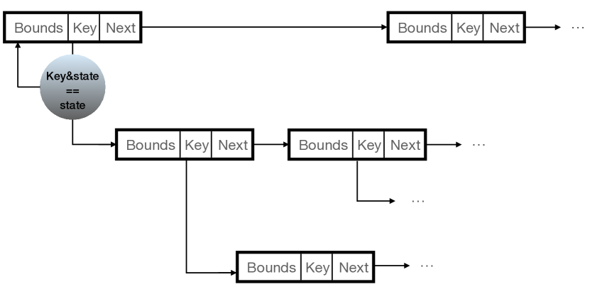
Figure 4: Illustration of a shallow tree structure used to store setrograde databases. The descent condition for a state lookup is superimposed on the path from the root node to its first child.

The maximum tree depth is the same as the retrograde depth, since 4 cards are defined at each level in the tree. Parents often have many children (the storage cost of each parent is split among its children) with the end effect that for each entry in the 24-card database, there are on average less than 2 (64 bit) nodes. Additionally, not all leaf nodes are at the maximum tree depth. x’s are implicitly represented, reducing the number of nodes per entry.

An independent tree is stored for each distribution of suits among the four players. This makes it practical to store the database in a compressed format, and expand only the portions of the database needed at any given point. Additionally, by reducing average tree size (by a factor of the Lower Bound in Table 1 — that is a factor of $2\times 10^{6}$ in the case of the 24 card database) we improve locality, and limit the cost of a query.

Several other small optimizations (child pointers are implicit, to save space; sibling pointers are relative) provide memory reductions and improve locality.

A state can be queried by starting from the root of a tree, and comparing the state’s 16-bit key (A state’s key has exactly one bit turned on for each 4-bit card representation) with a node’s 16-bit key using a bit-wise AND operator. If the bit-wise AND of the two keys is not equal to the state’s key, the state is not represented by the node. The lookup follows the sibling pointers until a match is found. When a match is found, the bounds are checked, and if a child exists, the search continues with the child.

Similar operations are used to look up sets, or given a set to find all dependent sets (sets sharing at least one state). Bit-wise operations are also used to find sets whose unions can be represented as a single set.

It is likely that the data structure could benefit from additional sorting, allowing for more direct access, however, the benefits of this data structure when compared with other structures we tried were crucial (and sufficient) for generating a 24-card database.

References

- Adelson-Velsky, Arlazarov, and Donskoy (1988) Adelson-Velsky, G. M.; Arlazarov, V. L.; and Donskoy, M. V. 1988. The Method of Analogy. Springer New York. ISBN 978-1-4612-3796-9.
- Beling (2017) Beling, P. 2017. Partition Search Revisited. IEEE Transactions on Computational Intelligence and AI in Games, 9(1): 76–87.
- Berlekamp and Wolfe (1994) Berlekamp, E.; and Wolfe, D. 1994. Mathematical Go: Chilling Gets the Last Point. AK Peters/CRC Press.
- Chess (2024) Chess. 2024. Syzygy Endgame Tablebases. syzygy-tables.info.
- Edelkamp, Kissmann, and Torralba (2015) Edelkamp, S.; Kissmann, P.; and Torralba, A. 2015. BDDs strike back (in AI planning). In Proceedings of the AAAI Conference on Artificial Intelligence, volume 29, 4320–4321.
- Furtak (2013) Furtak, T. 2013. Symmetries and Search in Trick-Taking Card Games. Ph.D. thesis, University of Alberta.
- Gaschnig (1979) Gaschnig, J. G. 1979. Performance measurement and analysis of certain search algorithms. Ph.D. thesis, Carnegie Mellon University.
- Ginsberg (1996) Ginsberg, M. 1996. Partition Search. In AAAI National Conference, 228–233.
- Haglund and Hein (2014) Haglund, B.; and Hein, S. 2014. Search algorithms for a bridge double dummy solver. privat.bahnhof.se/wb758135/bridge/Alg-dds˙x.pdf.
- Hart, Nilsson, and Raphael (1968) Hart, P.; Nilsson, N.; and Raphael, B. 1968. A Formal Basis for the Heuristic Determination of Minimum Cost Paths. IEEE Transactions on Systems Science and Cybernetics, 4(2): 100–107.
- Müller (2002) Müller, M. 2002. Proof-Set Search, 88–107. Springer.
- Romein and Bal (2003) Romein, J.; and Bal, H. 2003. Solving the Game of Awari using Parallel Retrograde Analysis. IEEE Computer, 38(10): 26–33.
- Schaeffer et al. (2007) Schaeffer, J.; Burch, N.; Björnsson, Y.; Kishimoto, A.; Müller, M.; Lake, R.; Lu, P.; and Sutphen, S. 2007. Checkers Is Solved. Science, 317(5844): 1518–1522.
- Schaeffer et al. (1992) Schaeffer, J.; Culberson, J.; Treloar, N.; Knight, B.; Lu, P.; and Szafron, D. 1992. A World Championship Caliber Checkers Program. Artificial Intelligence, 53(2-3): 273–290.
- Sturtevant (2003) Sturtevant, N. R. 2003. Multi-player games: Algorithms and approaches. Ph.D. thesis, UCLA.
- Sturtevant (2020) Sturtevant, N. R. 2020. On Strongly Solving Chinese Checkers. In Cazenave, T.; van den Herik, J.; Saffidine, A.; and Wu, I.-C., eds., Advances in Computer Games, 155–166. Cham: Springer International Publishing. ISBN 978-3-030-65883-0.
- Sturtevant and Saffidine (2017) Sturtevant, N. R.; and Saffidine, A. 2017. A Study of Forward Versus Backwards Endgame Solvers with Results in Chinese Checkers. In Computer Game Workshop at IJCAI, 121–136.