Injection process of pickup ion acceleration at an oblique heliospheric termination shock

Abstract

Injection process of pickup ion acceleration at a heliospheric termination shock is investigated. Using two-dimensional fully kinetic particle-in-cell simulation, accelerated pickup ions are self-consistently reproduced by tracking long time evolution of shock with unprecedentedly large system size in the shock normal direction. Reflected pickup ions drive upstream large amplitude waves through resonant instabilities. Convection of the large amplitude waves causes shock surface reformation and alters the downstream electromagnetic structure. A part of pickup ions are accelerated to tens of upstream flow energy in the time scale of $\sim 100$ times inverse ion gyro frequency. The initial acceleration occurs through shock surfing acceleration mechanism followed by shock drift acceleration mechanism. Large electrostatic potential accompanied by the upstream waves enables the shock surfing acceleration to occur.

1 Introduction

A collisionless shock is ubiquitous in space. It is an energy converter formed in a supersonic plasma flow. A variety of explosive phenomena in space, stellar wind, astrophysical jet accompany collisionless shocks. One of the outstanding issues of collisionless shock physics is the mechanism of particle acceleration occurring around it. It is believed that cosmic rays are produced in a collisionless shock through the diffusive shock acceleration (DSA) mechanism (e.g., Blandford & Eichler (1987)). In order for the DSA mechanism to work, preaccelerated nonthermal particles have to exist near a shock front. However, the mechanism producing such nonthermal particles, which should be dominated by complex microstructures of local electromagnetic fields, has been an open question for a long time. This is called the injection problem (Balogh & Treumann, 2013; Burgess & Scholer, 2015; Amano et al., 2022).

The heliospheric termination shock (HTS) is thought to be an ideal laboratory to study the injection process, because the anomalous cosmic rays (ACRs) having typically several tens of mega electron volts (MeV) are believed to be accelerated there (Chalov, 2006). However, the Voyager spacecraft observed only little amount of ACRs in the heliosheath, downstream of the HTS (e.g., Stone et al. (2005)). The reason for this was inferred by McComas & Schwadron (2006) as that efficient acceleration of ACRs occurs in the flank regions of the HTS, where geometrical condition of the local HTS is more suitable for particle acceleration than that of the HTS where the two Voyager spacecraft crossed.

On the other hand, Giacalone et al. (2021) recently performed hybrid (kinetic ions with charge neutralizing electron fluid) simulations and showed that the acceleration rate of low energy ($\lesssim 50$ keV) pickup ions (PUIs) is more or less independent of the position in the HTS. The nonthermal particles in this energy range are expected to have their global map obtained in the near future through the IMAP (Interstellar Mapping and Acceleration Probe) mission. In their simulation (Giacalone et al., 2021), turbulence in the solar wind is taken into account. Particles are expected to undergo scattering by the turbulent field, leading to some degree of acceleration, and there is a potential for these particles to be injected into the DSA process (Giacalone et al., 2021; Trotta et al., 2021; Pitňa et al., 2021; Zank et al., 2021; Trotta et al., 2022; Nakanotani et al., 2022; Wang et al., 2023). Another expected effect is the tilting of local magnetic field line. In oblique shocks particles reflected by the shock travel upstream, exciting waves themselves and generating mildly accelerated particles injected into the DSA process. Such a situation may occur in some specific regions of termination shock and perhaps locally everywhere when solar wind is turbulent. In this scenario, the generation of mildly accelerated particles needs to occur near the shock, but the detailed mechanism is not well understood. This study aims to validate the latter scenario.

It is thought that initial acceleration sets in when a particle is reflected at the shock. In general shock potential strongly affects the reflection of PUIs. In a hybrid simulation, the electrostatic potential is typically derived from a generalized Ohm’s law, which includes a term proportional to the electron pressure gradient. Calculating this electron pressure gradient term requires assuming a specific equation of state for electrons. Consequently, the electrostatic field in a hybrid simulation becomes model-dependent. Swisdak et al. (2023) pointed out that fully kinetic particle-in-cell (PIC) simulation leads to higher fluxes and maximal energies of PUIs than hybrid simulation likely due to differences in the shock potential. Before the Voyager spacecraft crossed the HTS, the shock surfing acceleration (SSA) was widely accepted as a plausible mechanism of injection (Lee et al., 1996; Zank et al., 1996). However, the Voyager did not observe the expected amount of high energy particles when they crossed the HTS (Decker et al., 2008). This implies that the shock surfing acceleration mechanism did not work effectively either. The reason for that SSA does not work in the termination shock was explained by Matsukiyo & Scholer (2014) by using one-dimensional fully kinetic particle-in-cell (PIC) simulation of (quasi-)perpendicular shock that most of potential jump in a PUI mediated shock occurs in an extended foot produced by reflected PUIs so that the potential jump at a shock ramp is insufficiently small for the SSA mechanism to work. The shock potential in an oblique PUI mediated shock has not been extensively studied so far.

Although the ab-initio PIC simulation is useful to reproduce complex multiscale electromagnetic structures responsible for injection processes, it requires large numerical cost. That is why PIC simulation of a collisionless shock in a plasma containing PUIs has been limitted mainly to the cases with one spatial dimension (e.g., Lee et al. (2005); Matsukiyo et al. (2007); Matsukiyo & Scholer (2011, 2014); Oka et al. (2011); Lembege & Yang (2016, 2018); Lembege et al. (2020)). Two-dimensional PIC simulations including PUIs are first conducted by Yang et al. (2015). They focused on the impact of PUIs on shock front nonstationarity of a perpendicular shock, $\Theta_{Bn}=90^{\circ}$, and energy dissipation up to $t=8\Omega^{-1}_{i}$, where $\Theta_{Bn}$ denotes the shock angle, the angle between shock normal and upstream magnetic field, and $\Omega_{i}$ is upstream ion cyclotron frequency. Kumar et al. (2018) performed longer simulation up to $t\sim 30\Omega^{-1}_{i}$ for quasi-perpendicular shocks, $\Theta_{Bn}=80^{\circ}$. They paid more attention to energy distribution of PUIs and solar wind ions (SWIs) for different upstream velocity distribution functions of PUIs. A little longer calculation up to $t\sim 40\Omega^{-1}_{i}$ was done with $\Theta_{Bn}=70^{\circ}$ by Swisdak et al. (2023). However, since the shock angle is close to or equal to perpendicular in the above previous studies, significant acceleration of PUIs are not reproduced. Indeed, when considering the average values, the shock angle of the termination shock is nearly perpendicular. However, as mentioned in the previous paragraph, it is easy to predict that the local shock angle fluctuates significantly due to the effects of solar wind turbulence and unsteady solar activity. This fluctuation could have important implications for the ion injection process.

In this study we focus the initial acceleration, which is often called injection process, of PUIs at an oblique HTS. The microstructures of a local oblique HTS with $\Theta_{Bn}=50^{\circ}$, and with $60^{\circ}$ and $70^{\circ}$ for comparison, mediated by the presence of PUIs and their impact on PUI acceleration are discussed by performing two-dimensional full PIC simulation with unprecedentedly long simulation time ($t_{max}=125\Omega^{-1}_{i}$).

2 PIC simulation

2.1 Settings

The system size in $x-y$ simulation domain is $L_{x}\times L_{y}=2,000v_{A}/\Omega_{i}\times 40.96v_{A}/\Omega_{i}$ which is divided by $200,000\times 4,096$ grid points. Here, $v_{A}$ denotes upstream Alfvén velocity. The so-called injection method is utilized to form a shock. An upstream homogeneous plasma consisting of solar wind electrons and ions as well as PUIs is continuously injected from the moving boundary at finite $x$, while the plasma and electromagnetic waves are reflected at the fixed rigid wall boundary at $x=0$. The simulation frame is a downstream plasma frame so that a shock propagates toward positive $x-$direction. Initially 20 particles per cell are distributed for each species. The distribution functions of the injected solar wind electrons and ions are a shifted-Maxwellian and that of the injected PUIs is a shifted-shell distribution with zero width of the shell velocity. The injection (or drift) speed is $-3.75v_{A}$ so that the Alfvén Mach number of the shock is $M_{A}\approx 5.5$ for $\Theta_{Bn}=50^{\circ}$, $M_{A}\approx 5.8$ for $\Theta_{Bn}=60^{\circ}$, and $M_{A}\approx 5.9$ for $\Theta_{Bn}=70^{\circ}$, respectively. Here, the upstream magnetic field is in the $x-y$ simulation plane. These values of the Mach number are close to the one estimated by Li et al. (2008) using Voyager 2 data, while is a little smaller than the value assumed in Giacalone et al. (2021). The upstream electron beta is $\beta_{e}=0.25$ and the solar wind ion temperature is the same as that of electrons, $T_{i}=T_{e}$. The beta value is slightly larger than the estimates by Li et al. (2008) and the values assumed by Giacalone et al. (2021), but considering the significant variations in solar wind temperature observed by Voyager 2 (Richardson et al., 2008), it falls within a realistic range. The ion to electron mass ratio is $m_{i}/m_{e}=100$ for both the SWIs and PUIs, the ratio of upstream electron plasma frequency to cyclotron frequency $\omega_{pe}/\Omega_{e}=4$, and the relative PUI density is 25%, respectively. In the following, the run with $\Theta_{Bn}=50^{\circ}$ is mainly discussed. Hereafter, time is normalized to $\Omega^{-1}_{i}$, velocity to $v_{A}$, and distance is to $v_{A}/\Omega_{i}$, respectively.

2.2 Overview

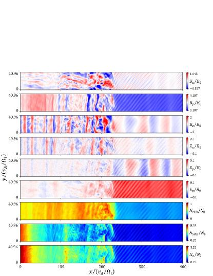
Figure 1: Structure of a PUI mediated oblique shock at $t=125$ ($\Theta_{Bn}=50^{\circ}$). From the top, the first three panels denote magnetic field $B_{x},B_{y},B_{z}$, the next three panels electric field $E_{x},E_{y},E_{z}$, and the last three indicate density of PUIs ($N_{\rm PUI}$), SWIs ($N_{\rm SWI}$), and electrons ($N_{e}$), respectively.

Fig.1 shows the structure of a shock at $t=125$, where a shock ramp is at $x\sim 210$. The first three panels represent magnetic field $B_{x},B_{y},B_{z}$, the next three electric field $E_{x},E_{y},E_{z}$, and the last three indicate density of PUIs ($N_{\rm PUI}$), SWIs ($N_{\rm SWI}$), and electrons ($N_{e}$), respectively. Both upstream and downstream, large amplitude waves are generated.

Liu et al. (2010) showed by performing a 2D hybrid simulation of a perpendicular shock including 20% PUIs that Alfvén ion cyclotron (AIC) instability and mirror instability lead to the downstream turbulent field. The AIC waves are visible in $B_{x}$ and $B_{z}$ and mainly propagate along the downstream magnetic field, while the mirror waves have wavenumbers oblique to it and are the most visible in $B_{y}$. In Fig.1, however, the AIC wave signature is confirmed only in $B_{x}$. The signature of mirror waves in $B_{y}$ and that of AIC waves in $B_{z}$ are overwhelmed by the vertical stripes which are also seen in $E_{x}$ and $E_{y}$.

The upstream waves are dominated by two types, a relatively long wavelength waves propagating in negative $x-$direction (vertical stripes) and a relatively short wavelength waves propagating in almost perpendicular to the ambient magnetic field (oblique stripes). These waves are convected by the upstream flow. The former are not only the origin of the downstream vertical structures discussed above, but also the cause of shock surface reformation. We will discuss the generation mechanism of the upstream waves below.

2.3 Upstream waves

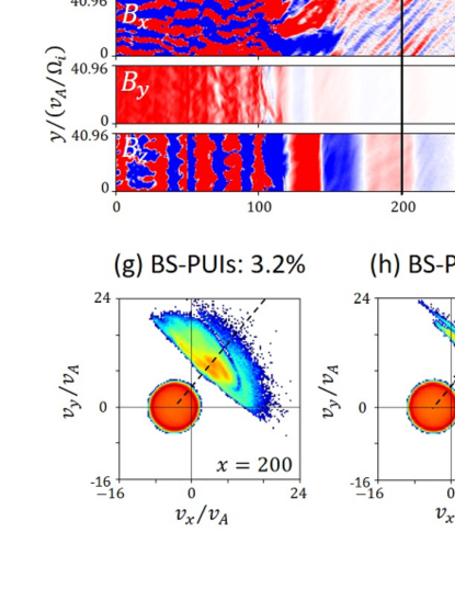
Figure 2: Particle distribution and magnetic fields upstream of the shock at $t=65$ ($\Theta_{Bn}=50^{\circ}$). From the top, $V_{x}-x$ phase space distributions of (a) PUIs, (b) solar wind ions, (c) electrons, magnetic field components of (d) $B_{x}$, (e) $B_{y}$, (f) $B_{z}$, velocity distributions of PUIs at (g) $x=200$, (h) $x=300$, and (i) $x=400$, respectively. In (a-c) and (g-i), only the particles at $y\approx L_{y}/2$ are counted. The color bars in (a-c) denote phase space density (in an arbitrary unit). The color bar in (g-i) denote velocity space density (in an arbitrary unit). The dashed lines in (g-i) represent the direction of local (upstream) magnetic field, ${\bf B_{0}}$.

In Fig.2 the $V_{x}-x$ phase space distributions of (a) PUIs, (b) SWIs, and (c) electrons, whose positions in $y$ are $y\approx L_{y}/2$, are shown, the corresponding magnetic field structures are represented in (d-f), and velocity space distributions of the PUIs at different positions in $x$ are indicated in (g-i), respectively, at $t=65$. The color scale in (a-c) and in (g-i) are in an arbitrary unit, and the color scale of the magnetic field is adjusted to appropriately see the upstream structures. It is clearly seen in (a) that some PUIs are reflected and backstreaming from the shock front at $x\approx 105$ toward upstream. On the other hand, as in the previous kinetic simulations of PUI mediated shocks (Matsukiyo & Scholer, 2014; Wu et al., 2009), no SWIs are reflected (b). This implies that the upstream waves are generated by these backstreaming PUIs (BS-PUIs). In the local velocity space at (g) $x=200$, (h) $x=300$, and (i) $x=400$, the red circular populations denote incoming PUIs, while the BS-PUIs are indicated by the rest in each panel. The BS-PUIs are well separated in the velocity space from the incoming PUIs and their average velocities roughly align to the black dashed lines indicating the direction of upstream magnetic field. The relative density of the BS-PUIs is 0.3% at $x=400$, 1.3% at $x=300$, and 3.2% at $x=200$, respectively.

Since the BS-PUIs are regarded as a field aligned beam, linear dispersion analysis of a beam-plasma system including background ions, electrons, and beam ions is performed. The details of the analysis are provided in the appendix.

In Fig.3 two unstable solutions obtained by solving the linearized Vlasov-Maxwell equation system are depicted. One is for $\theta_{Bk}=50^{\circ}$ and another is for $\theta_{Bk}=87^{\circ}$, where $\theta_{Bk}$ is the wave propagation angle with respect to the ambient magnetic field. For each solution, the solid line denotes the real part of frequency, while the dashed line shows the imaginary part. For $\theta_{Bk}=50^{\circ}$, the maximum growth rate occurs at $k\approx 0.096$. This corresponds to the relatively long wavelength waves having a wavenumber along the $x-$axis seen in Fig.2(e-f). The maximum growth rate occurs at $k\approx 1.2$ for $\theta_{Bk}=87^{\circ}$, which corresponds to the relatively short wavelength waves seen in Fig2(d). These instabilities are interpreted as a resonant instability with oblique propagation angle.

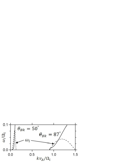
Figure 3: Linear dispersion relation of oblique resonant instability driven by BS-PUIs.

2.4 Injection of PUIs

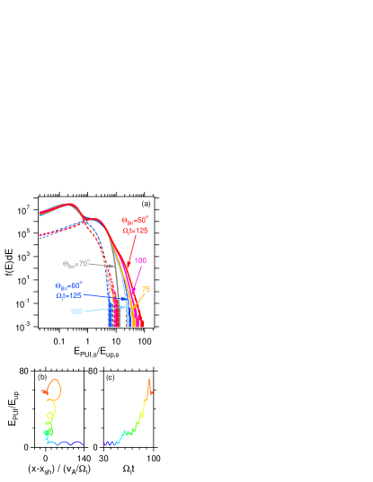
Figure 4: (a) Energy distributions of downstream PUIs at various shock angles and times. Each distribution (solid line) is divided into the two dashed lines indicating SWIs (lower energy) and PUIs (higher energy). Energy history of an accelerated PUI is shown by the rainbow colored lines as a function of (b) space and (c) time, respectively. The line color denotes time.

Fig.4(a) shows downstream energy distribution functions of ions at different times, $t=75$ (orange), 100 (magenta), and 125 (red), where the energy is measured in the shock rest frame and normalized to the upstream bulk flow energy. The each solid line, indicating the distribution of whole ions, is divided into the two dashed lines with relatively low and high energy. The low and high energy ones denote solar wind ions and PUIs, respectively. It is evident that high energy tail of the PUIs evolves in time, indicating the system has not reached steady evolution state with a constant power-law index.

For comparison, simulations for $\Theta_{Bn}=70^{\circ}$ and $\Theta_{Bn}=60^{\circ}$ were additionally performed. At $\Theta_{Bn}=70^{\circ}$, no backstreaming ions were observed, and the downstream energy distribution remained steady during the same time interval, with no discernible accelerated component of PUIs. The energy distribution at this time ($t=125$) is shown by the gray line. At $\Theta_{Bn}=60^{\circ}$, a very small amount of backstreaming ions was observed. As indicated by blue and cyan lines in Fig.4(a), the generation of accelerated PUIs can be observed over time, but the generation efficiency is evidently lower than that at $\Theta_{Bn}=50^{\circ}$. The energy densities of accelerated particles at $t=125$, relative to the steady downstream plasma energy density at $\Theta_{Bn}=70^{\circ}$, are 0.066 when $\Theta_{Bn}=60^{\circ}$ and 0.13 when $\Theta_{Bn}=50^{\circ}$, respectively. We consider the shock angle of $60^{\circ}$ to be close to the critical angle where particle backstreaming begins. At $\Theta_{Bn}=50^{\circ}$, the excitation of large-amplitude upstream waves by backstreaming PUIs is believed to increase the efficiency of accelerated PUI generation as discussed below.

The flux at the shoulder of the accelerated PUIs is roughly two orders of magnitude lower than the peak flux of PUIs. This relative flux of the shoulder looks comparable to or even higher than that seen in the past hybrid simulation with higher $M_{A}$ (Giacalone et al., 2021). To explore the potential reasons for this difference, attention is drawn to the initial behavior of the accelerated particles. Evolution of energy of an accelerated PUI is depicted by the rainbow colored lines in Fig.4(b) and (c) as a function of relative distance from the shock and time, respectively. Here, $x_{sh}$ is the shock position averaged in the $y$ direction and the energy is measured in the simulation (downstream) frame. The PUI shows typical cycloidal motion up to $t\sim 50$. Once it is reflected, the PUI starts gaining energy. Beyond $t\sim 60$, there is an increase in energy accompanied by periodic fluctuations, indicative of shock drift acceleration (SDA) characteristics. In SDA, an ion gyrating across a shock has relatively small gyro radius behind a ramp and large gyro radius in front of it so that the ion drifts along the shock surface parallel to the motional electric field. The small gyro motion behind a ramp is denoted in Fig.4(b) as the loop orbit. The same type of trajectory is reported by Giacalone & Decker (2010) (see their Fig.3). However, upon careful observation of the trajectory, it is evident that there is another acceleration phase before $t\sim 60$ and the behavior of the particle during this phase differs from that observed afterward. When first reflected at $x\approx x_{sh}$, the particle exhibits a trajectory that is not loop-like, indicating that the reflection occurs due to potential. The subsequent second reflection is also similar, and such multiple reflections due to potential followed by incomplete gyro-motion are characteristic of SSA.

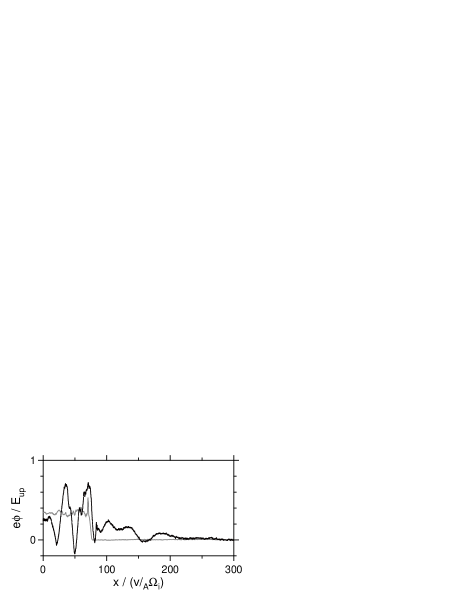
Figure 5: Electrostatic potential for $\Theta_{Bn}=50^{\circ}$ (black) and $\Theta_{Bn}=70^{\circ}$ (gray) at $t=50$ along $y\approx 27$. The gray line is shifted horizontally in $x$ to align the overshoot position with that of the black line.

Here, the SSA can work because of the large amplitude upstream waves. The black line in Fig.5 represents the profile of electrostatic potential normalized to upstream flow energy, $e\phi/E_{\rm up}$, along $y\approx 27$ at $t=50$ which is close to the time and position in $y$ when the PUI in Fig.4(b,c) was first reflected at the shock. The fluctuation of potential is clearly seen both upstream and downstream of the shock ramp ($x\approx 80$). The upstream fluctuation is compressed and amplified at the shock. The potential occurs about 0.2 $E_{\rm up}$ at $x\approx 100$ already before the ramp. At the ramp, large jump is seen so that the potential reaches nearly 0.7 $E_{\rm up}$. For comparison, the potential at $\Theta_{Bn}=70^{\circ}$ at the same time is indicated by the gray line. Here, the $x$-value is shifted to align the overshoot position almost the same. Without backstreaming ions and upstream large amplitude waves, both foot by the reflected PUIs and steep ramp can be observed (although not clear in this scale). The potential increase at the foot is about 0.3 $E_{up}$, and its spatial scale is approximately the gyro radius of the reflected PUIs, and the gradient of the potential in this part is smaller than that of the ramp at $\Theta_{Bn}=50^{\circ}$. The potential increase at the ramp is slightly over 0.2 $E_{\rm up}$, and the total potential increase is smaller than that of $\Theta_{Bn}=50^{\circ}$. Note that the obliquely propagating waves contain electrostatic field component. Therefore, the large amplitude upstream waves accompany electrostatic potential. When $\Theta_{Bn}=50^{\circ}$, the waves are compressed at the shock so that the gradient of potential increases. The potential jump at the ramp occurs within a few ion inertial lengths, although it is larger than the electron inertial length which was originally assumed by Lee et al. (1996). Furthermore, the density increase due to the shock compression amplifies the potential. These effects can cause the observed SSA of the PUI and this additional acceleration occurring immediately after the first reflection may enhance the production rate of the accelerated PUIs. Although we didn’t investigate all particles, we confirmed that among the particles we examined, those with exceptionally high energy ($E_{\rm PUI}/E_{\rm up}>60$ at $t=100$) underwent the SSA process before the SDA process.

3 summary

We investigated injection process of PUI acceleration at a PUI mediated oblique shock by using two-dimensional PIC simulation. The evolution of system with sufficiently large spatial size in the shock normal direction was followed for sufficiently long time ($t>100$) to reproduce accelerated PUIs for the first time. Backstreaming PUIs drive large amplitude waves through resonant instabilities. The convection of those large amplitude waves causes shock surface reformation and alters the downstream structure. A part of PUIs are accelerated to tens of upstream flow energy with the time scale of $t\sim 100$ as observed in hybrid simulation by Giacalone et al. (2021). The initial acceleration occurs through SSA mechanism followed by SDA mechanism. The electrostatic potential accompanied by the large amplitude upstream waves enables the SSA to occur.

McComas & Schwadron (2006) argue that low-energy particles are more likely to be accelerated at the terminal shocks in the flank of the heliosphere, where shock angles are oblique. The results discussed here qualitatively support this claim. However, the acceleration of particles in the tens of keV range discussed here requires shock angles of approximately $60^{\circ}$ or less for injection, whereas typical shock angles at the flank may not be so small. It may be that the solar wind turbulence advocated by Giacalone et al. (2021); Giacalone & Decker (2010) is necessary for injection.

Due to the finite system length in the $y-$direction, only limited wave modes are allowed to grow in our simulation. In the real system there should be other unstable wave modes with different $\theta_{Bk}$. Those waves may lead to efficient scattering of the accelerated PUIs, which should be confirmed in future. The accelerated particles in the tens of keV ($\sim$tens of upstream flow energy) range observed at $\Theta_{Bn}=50^{\circ}$ correspond to the energy range of energetic neutral atoms targeted by IMAP (Interstellar Mapping and Acceleration Probe) mission, and valuable insights into the particle injection site may be obtained from the data of its all-sky map.

Appendix

The dispersion relation of upstream waves (Fig.3) are obtained by numerically solving the linearized Vlasov-Maxwell equation system. The detailed derivation of the dispersion equation including a beam component at oblique propagation is given in Chap.8 of Gary (2005).

We assumed that there are three species, background ions, electrons, and beam ions. Each distribution function follows a (shifted-)Maxwellian distribution. The thermal velocity of electrons is 3.5, corresponding to an electron beta of 0.25. The electrons are given a drift velocity along the magnetic field to cancel out the current created by the beam ions. The background ions include both SWIs and PUIs, although we do not distinguish between the two and treat them as a single component of background ions at rest with an effective thermal velocity of 2.7. This value corresponds to an effective ion beta of 15, which is the sum of SWI beta and PUI beta. We will discuss the validity of this assumption later. As shown in Fig.2, the drift velocity of the beam ions varies depending on the distance from the shock. Here, a representative value of 16 is used. The thermal velocity of beam ions is set to $v_{tb}=1$. The beam population is actually propagating along the magnetic field with finite pitch angle so that the distribution function is a ring-beam type. This is the reason why the beam population in Fig.2(i) looks anisotropic in the velocity space. Since the ring velocity is clearly smaller than the beam velocity, we neglect the ring velocity in the dispersion analysis. Furthermore, a relative beam density of 0.3% is used. As long as the relative density is sufficiently small, the wavelength of the excited waves is hardly affected by it. The analysis is done in the frame of background ions.

Fig.3 is obtained with the above conditions. For $\theta_{Bk}=50^{\circ}$, the maximum growth rate occurs at $k\approx 0.096$ and $\omega\approx 0.07$. Since the argument of plasma dispersion function, $\zeta_{b}=(\omega-{\bf k\cdot v_{b}}+\Omega_{i})/\sqrt{2}k_{\parallel}v_{tb}$, is estimated as $\approx 0.95(<1)$, the observed instability is a resonant instability. For $\theta_{Bk}=87^{\circ}$, the maximum growth rate occurs at $k\approx 1.2$ and $\omega\approx 0.065$, leading to $\zeta_{b}\approx 0.68(<1)$. Hence, the instability is also a resonant instability. Fig.6 shows the dependence of the dispersion relation on the beta of the background ions, $\beta_{i}$. For both $\theta_{Bk}=50^{\circ}$ and $87^{\circ}$ cases, the maximum growth rate and the corresponding wavenumber do not very change, while $\beta_{i}$ varies from 0.25 to 15. This indicates that our assumption of considering SWIs and incoming PUIs as a single background ion component was valid.

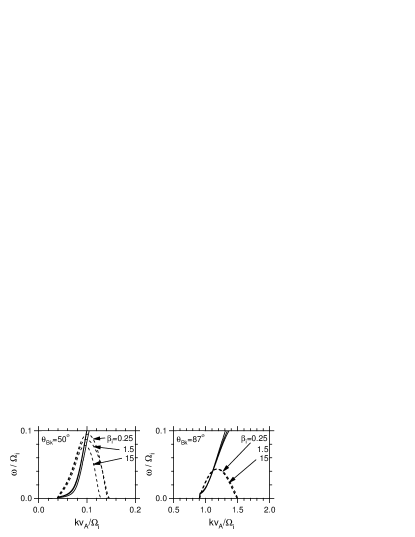
Figure 6: Linear dispersion relation of oblique resonant instability driven by BS-PUIs with different background ion beta, $\beta_{i}$. The solid and dashed lines indicate real and imaginary parts of frequency, respectively.

References

- Amano et al. (2022) Amano, T., Matsumoto, Y., Bohdan, A., et al. 2022, Rev. Mod. Plasma Phys., 6, 29
- Balogh & Treumann (2013) Balogh, A., & Treumann, R. A. 2013, Physics of Collsionless Shocks (Springer)
- Blandford & Eichler (1987) Blandford, R., & Eichler, D. 1987, Phys. Rep., 154, 1
- Burgess & Scholer (2015) Burgess, D., & Scholer, M. 2015, Collisionless Shocks in Space Plasmas (Cambridge University Press)
- Chalov (2006) Chalov, S. 2006, in The Physics of the Heliospheric Boundaries, ed. V. Izmodenov & R. Kallenbach, Vol. 5 (International Space Science Institute), 245
- Decker et al. (2008) Decker, R. B., Krimigis, S. M., Roelof, E. C., et al. 2008, Nature, 454, 67
- Gary (2005) Gary, S. P. 2005, Theory of Space Plasma Microinstabilities (Cambridge University Press)
- Giacalone & Decker (2010) Giacalone, J., & Decker, R. 2010, Astrophys. J., 710, 91
- Giacalone et al. (2021) Giacalone, J., Nakanotani, M., Zank, G. P., et al. 2021, Astrophys. J., 911, 27
- Kumar et al. (2018) Kumar, R., Zirnstein, E. J., & Spitkovsky, A. 2018, Astrophys. J., 860, 156
- Lee et al. (1996) Lee, M., Shapiro, V. D., & Sagdeev, R. Z. 1996, J. Geophys. Res., 101, 4777
- Lee et al. (2005) Lee, R. E., Chapman, S. C., & Dendy, R. O. 2005, Ann. Geophys., 23, 643
- Lembege & Yang (2016) Lembege, B., & Yang, Z. 2016, Astrophys. J., 827, 73
- Lembege & Yang (2018) —. 2018, Astrophys. J., 860, 84
- Lembege et al. (2020) Lembege, B., Yang, Z., & Zank, G. P. 2020, Astrophys. J., 890, 48
- Li et al. (2008) Li, H., Wang, C., & Richardson, J. D. 2008, Geophys. Res. Lett., 35, L19107
- Liu et al. (2010) Liu, K., Gary, P., & Winske, D. 2010, J. Geophys. Res., 115, A12114
- Matsukiyo & Scholer (2011) Matsukiyo, S., & Scholer, M. 2011, J. Geophys. Res., 116, A08106
- Matsukiyo & Scholer (2014) —. 2014, J. Geophys. Res., 119, 2388
- Matsukiyo et al. (2007) Matsukiyo, S., Scholer, M., & Burgess, D. 2007, Ann. Geophys., 25, 283