Abstract

We explore the trade-off between privacy and statistical utility in private two-sample testing under local differential privacy (LDP) for both multinomial and continuous data. We begin by addressing the multinomial case, where we introduce private permutation tests using practical privacy mechanisms such as Laplace, discrete Laplace, and Google’s RAPPOR. We then extend our multinomial approach to continuous data via binning and study its uniform separation rates under LDP over Hölder and Besov smoothness classes. The proposed tests for both discrete and continuous cases rigorously control the type I error for any finite sample size, strictly adhere to LDP constraints, and achieve minimax separation rates under LDP. The attained minimax rates reveal inherent privacy-utility trade-offs that are unavoidable in private testing. To address scenarios with unknown smoothness parameters in density testing, we propose an adaptive test based on a Bonferroni-type approach that ensures robust performance without prior knowledge of the smoothness parameters. We validate our theoretical findings with extensive numerical experiments and demonstrate the practical relevance and effectiveness of our proposed methods.

1 Introduction

Large-scale internet services such as Netflix and Amazon collect sensitive data from massive user bases, allowing companies to conduct cost-effective randomized experiments by assigning users to two different user interfaces or marketing campaigns. By testing whether the resulting two independent sets of samples originate from the same distribution—a procedure known as A/B testing or two-sample testing—companies can statistically assess the impact of new interfaces or campaigns on various user behaviors. However, the sensitivity of detailed personal data raises substantial privacy concerns in data analysis. Since privacy protection inherently conceals some of the information in the data and in turn compromises statistical utility, it is crucial to characterize and balance the trade-off between statistical utility and data privacy. Differential privacy (DP; Dwork et al.,, 2006) provides a rigorous framework for this trade-off, defining data privacy as a mathematical concept that supports such balancing.

We briefly review two notions of DP: central DP and local DP (LDP; Kasiviswanathan et al.,, 2011). The central DP constraint, illustrated in Figure 1(a), assumes that a trusted data curator (or distributor) has access to the entire original data set and calculates a noisy statistical result. This centralized approach requires that the probability of any event remains essentially the same when a single data entry is arbitrarily perturbed. Under this constraint, one cannot reliably extract any individual-level information from the noisy statistical result. In contrast, under the local DP constraint, illustrated in Figure 1(b), data owners do not place trust in the curator. Instead, each data owner independently reports a noisy version of their data. This more stringent local constraint inevitably impairs statistical utility more than the central constraint. However, it provides a higher level of privacy and separates the data curator from the responsibility for disclosure risk.

These benefits have driven widespread adoption of the LDP framework in the internet-scale deployment of data analysis under privacy, such as in Apple (Apple Differential Privacy Team,, 2017), Google (Erlingsson et al.,, 2014), Microsoft (Ding et al.,, 2017), and Uber (Near,, 2018). With the massive user bases, these companies require stringent privacy protections, while also having the capacity to obtain large samples which allow statistically meaningful analyses within strong privacy constraints. Various implementations of LDP in industrial applications has naturally spurred a substantial body of work (Acharya et al., 2021d, ; Duchi et al.,, 2018; Lam-Weil et al.,, 2022; Lalanne et al.,, 2023; Cai et al.,, 2021), examining the intrinsic trade-off between privacy and statistical utility in various settings. Our paper contributes to the existing body of work by exploring this trade-off in the context of the two-sample testing problem.

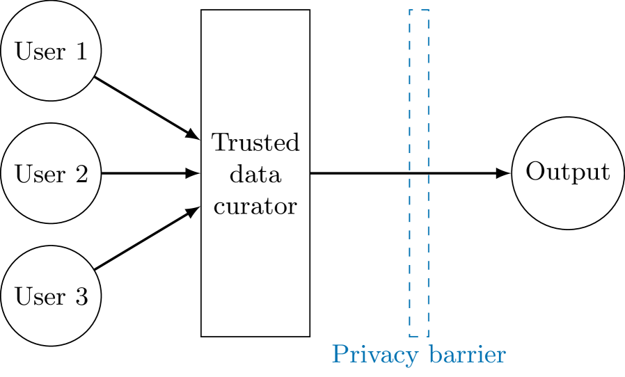
(a) Central differential privacy

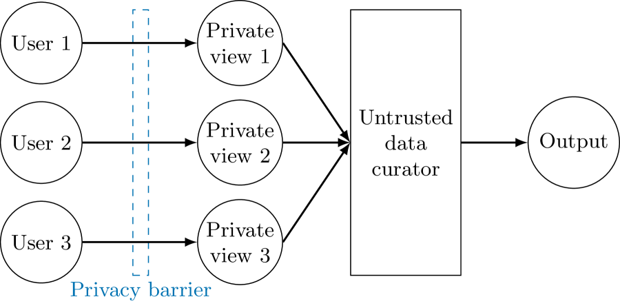
(b) Local differential privacy

Figure 1: Graphical illustration of central differential privacy and local differential privacy.

The two-sample testing problem, which originates from the classical two-sample $t$-test (Student,, 1908), has gained renewed interest in recent years due to the emergence of high-dimensional and complex data. Notably, several novel methodological approaches have been developed including kernel-based tests (Gretton et al.,, 2009, 2012), distance-based tests (Székely and Rizzo,, 2004, 2005) and regression/classification-based tests (Kim et al.,, 2019, 2021), which have demonstrated promising capabilities in dealing with modern data sets. On the theoretical front, researchers have explored the fundamental limit of this problem through the lens of minimax analysis both in the statistics (for example, Arias-Castro et al.,, 2018; Kim et al., 2022a, ; Schrab et al.,, 2023) and computer science (for example, Batu et al.,, 2000; Chan et al.,, 2014; Diakonikolas and Kane,, 2016; Goldreich and Ron,, 2011) literature. In addition to the methodological and theoretical advancements, the topic has found contemporary applications such as in education research (Rabin et al.,, 2019), network traffic analysis (Kohout and Pevný,, 2018), and audio segmentation (Harchaoui et al.,, 2009). Despite its long history and fundamental roles in practice, most of the existing work on two-sample testing has focused on non-private settings with a few exceptions. Exceptions include private versions of multinomial tests (Acharya et al.,, 2018; Aliakbarpour et al.,, 2019, 2018), traditional non-parametric tests (for example, Mann-Whitney and Wilcoxon signed-rank tests; Couch et al.,, 2019; Task and Clifton,, 2016), partitioning-based test of univariate continuous distributions (Sheffet and Omer,, 2024) and kernel tests (Raj et al.,, 2020; Kim and Schrab,, 2023) under central DP. The literature on two-sample testing under LDP is even more scarce. Notable contributions in this area include Ding et al., (2018) and Waudby-Smith et al., (2023), both of which are mainly concerned with detecting differences in location. In contrast, our primary goal is to develop two-sample tests for general alternatives under LDP, focusing on both multinomial and multivariate continuous data. Additionally, we shed new light on the fundamental limits of the two-sample problem under LDP.

In the following subsection, we begin with a review of related work and then discuss our techniques and contributions.

1.1 Related Prior Work

Private hypothesis testing has been extensively studied in the statistics and computer science literature. Among various studies on this topic, we briefly review those closely related to our work. Initially motivated by the privacy attack on genome-wide association study (GWAS) (Homer et al.,, 2008), the early work on private testing mainly concentrates on private versions of chi-square tests and explores their asymptotic properties (Gaboardi et al.,, 2016; Gaboardi and Rogers,, 2018; Johnson and Shmatikov,, 2013; Rogers and Kifer,, 2017; Uhler et al.,, 2013; Vu and Slavkovic,, 2009; Wang et al.,, 2015; Yu et al.,, 2014). In contrast, a recent line of work in computer science is concerned with non-asymptotic properties of private tests designed for multinomial data sets, and studies optimal sample complexities of testing problems from a minimax perspective. This line of work has been initiated by Cai et al., (2017) for central DP and Sheffet, (2018) for LDP, and continued by Acharya et al., (2018), Aliakbarpour et al., (2019, 2018), and Sheffet and Omer, (2024) for central DP and Acharya et al., (2020); Acharya et al., 2021a for LDP, respectively. The optimal sample complexity is usually achieved through a systematic analysis of both its upper and lower bounds. For the upper bound analysis, the prior works extend non-private multinomial tests, such as in Acharya et al., (2015), Chan et al., (2014), Diakonikolas et al., (2018), Diakonikolas and Kane, (2016), Goldreich and Ron, (2011), and Valiant and Valiant, (2014), to corresponding private counterparts by incorporating randomization mechanisms. On the other hand, the lower bound analysis relies on information-theoretic techniques, such as Le Cam’s method, while treating the DP requirement as information constraints (see, for example, Acharya et al.,, 2020; Duchi et al.,, 2018, for detailed discussions).

There are also a few recent papers from the statistics community that explore univariate goodness-of-fit testing under LDP. Specifically, Dubois et al., (2023) propose minimax optimal goodness-of-fit tests for Hölder densities under LDP in both non-interactive and interactive scenarios. Lam-Weil et al., (2022) also consider goodness-of-fit testing under LDP, and develop minimax optimal tests for multinomials and for continuous densities over Besov balls. Our work builds on their framework and extends the focus from goodness-of-fit testing to two-sample testing for both (i) multinomials and (ii) multivariate Hölder and Besov densities. It is worth highlighting that previous works (Lam-Weil et al.,, 2022; Dubois et al.,, 2023) rely solely on the Laplace mechanism (Dwork and Roth,, 2013) to establish their theoretical results. In contrast, we explore various LDP mechanisms that achieve similar optimality properties and empirically demonstrate that the Laplace mechanism can underperform in practical scenarios. Specifically, we delve into the Google’s RAPPOR (Erlingsson et al.,, 2014), generalized randomized response (Gaboardi and Rogers,, 2018), and (discrete) Laplace mechanisms (Ghosh et al.,, 2009), and illustrate their theoretical and empirical performance.

1.2 Techniques and Results

Previous work on hypothesis testing under local differential privacy has primarily focused on goodness-of-fit testing (Dubois et al.,, 2023; Lam-Weil et al.,, 2022). We instead target a broader and arguably more challenging settings of two-sample testing of multinomials and multivariate densities. In particular, we provide testing methods that are both practically reliable and theoretically optimal. Our practical reliability stems from both the privatization mechanism and the testing procedure. For privatization, one of our methods leverages Google’s RAPPOR, a widely adopted open-source privacy mechanism which has demonstrated effectiveness through years of large-scale deployment in Chrome browser. Although prior works (Duchi et al.,, 2013; Acharya et al.,, 2019; Acharya et al., 2021c, ) adopt RAPPOR and analyze its statistical performance under the minimax framework, their focuses are limited to $\ell_{1}$ separation and multinomial data. Our work expands upon them by establishing minimax optimality for both multivariate continuous and multinomial data under $\ell_{2}$ separation, marking the first result of its kind. For the testing procedure, our methods rigorously control the type I error in all scenarios. At the heart of achieving the blend of practicality and theory lies the permutation test. Achieving practical reliability poses a significant challenge, especially in calibrating the critical value within the non-asymptotic regime while accounting for the randomization effects introduced by local differential privacy. Under a composite null hypothesis of two-sample testing, critical values cannot be determined through Monte-Carlo-approximated population quantile of test statistics, unlike in goodness-of-fit testing. The critical values obtained through concentration inequalities, on the other hand, usually depend on unspecified constants and thus are not reliable in practice. By employing a permutation procedure, our testing methods guarantee type I error control at any sample size and with sufficiently large number of permutations (which does not depend on the sample size). The permutation procedure also facilitates theoretical analysis of power, leading to minimax upper bound analyses. In particular, it enables us to leverage the technique of Kim et al., 2022a , namely the two moments method therein. This technique allows us to avoid directly analyzing the permutation distribution under LDP, and provides a sufficient condition for type II error control based solely on the first two moments of the test statistic. Equipped with this tool, we analyze our test statistics, which are U-statistics derived from perturbed data with a carefully selected perturbation level. A bulk of our technical effort is dedicated to bounding the moments related to the U-statistic in the presence of this data perturbation.

By obtaining matching information-theoretic lower bounds, we establish the optimality of our methods and gain insight into the fundamental trade-off between statistical power and privacy. For the lower bound analysis, we leverage a recently developed technique by Lam-Weil et al., (2022). This technique builds upon Ingster’s method (Ingster,, 1993), a classical approach for deriving minimax separation rates in testing problems, and adapts it to incorporate the LDP constraint. At the heart of Ingster’s method is bounding the chi-square divergence between a simple null distribution and a mixture of alternative distributions. The key idea behind obtaining a tight lower bound under LDP is to construct a mixture distribution in Ingster’s method using the singular values and singular vectors of the privacy mechanism. Such construction naturally imposes extra restrictions caused by the LDP constraint, enabling us to achieve a tight lower bound under LDP. Our technical effort lies in extending the univariate result of Lam-Weil et al., (2022) to more general settings, including the multivariate Hölder ball and Besov ball.

Summary of our contributions. We highlight our contributions and contrast them with prior work as follows. We also refer readers to Table 1, which summarizes the non-private and private minimax separation rates for two-sample testing, derived from both prior work and our findings.

	Non-private rate	Private rate under LDP
Testing for multinomials in $\ell_{2}$ separation	$n_{1}^{-1/2}$ (Chan et al.,, 2014; Kim et al., 2022a, )	$\dfrac{k^{1/4}}{{(n_{1}\alpha^{2})^{1/2}}}\vee n_{1}^{-1/2}$ (Theorem 3.1)
Testing for Hölder and Besov densities in $\mathbb{L}_{2}$ separation	$n_{1}^{\frac{-2s}{4s+d}}$ (Arias-Castro et al.,, 2018)	$(n_{1}\alpha^{2})^{\frac{-2s}{4s+3d}}\vee n_{1}^{\frac{-2s}{4s+d}}$ (Theorem 4.1)

Table 1: Non-private and private minimax rates for two-sample multinomial and density testing in $\ell_{2}$ and $\mathbb{L}_{2}$ separation where $n_{1}$ denotes the minimum sample size and $\alpha$ denotes the privacy level. For multinomial testing, $k$ stands for the number of categories, and for density testing, $s$ represents the smoothness parameter. The rates exhibit elbow effects—phase transitions at specific levels of privacy. See Section 3 and 4 for details.

• Optimal multinomial testing under LDP (Theorem 3.1): We start by developing a private two-sample test for multinomials, and present minimax separation rates in terms of the $\ell_{2}$ distance under LDP. The prior work (Acharya et al.,, 2018; Aliakbarpour et al.,, 2019, 2018) for private two-sample testing generally focuses on central DP and imposes conditions such as equal sample sizes and Poisson sampling that may not be practically relevant. In contrast, our approach does not rely on such unnecessary conditions, and obtain optimality under more practical settings. We also highlight that our upper bound result is established using three distinct LDP mechanisms—namely Laplace, discrete Laplace and RAPPOR mechanisms—which diversifies the toolkit in practice. As mentioned earlier, this is in contrast to the prior work (Lam-Weil et al.,, 2022; Dubois et al.,, 2023), which mainly focuses on the Laplace mechanism. Moreover, we show that the use of generalized randomized response mechanism (Gaboardi and Rogers,, 2018) can lead to suboptimal power in Appendix H.

• Optimal density testing under LDP (Theorem 4.1): We next consider the two-sample problem for continuous data and derive optimal $\mathbb{L}_{2}$ separation rates under LDP, by leveraging the prior work (Lam-Weil et al.,, 2022; Kim et al., 2022a, ). In particular, we examine both Hölder and Besov smoothness classes, and show that the proposed private test is optimal for both classes with the finite-sample validity. This approach differs from the prior work on a similar topic. For instance, unlike Sheffet and Omer, (2024) that consider central DP with Poissonization, we focus on the more stringent setting of LDP and consider the standard sampling with fixed sample sizes. Moreover, in contrast to the prior work under LDP (Ding et al.,, 2018; Waudby-Smith et al.,, 2023), primarily focused on location alternatives, our private test is sensitive against a broad range of nonparametric alternatives. Lastly, we highlight that our method controls the type I error in any finite sample sizes, and exactly satisfies the LDP condition, distinguishing it from the prior work of Raj et al., (2020).

• Adaptive density testing under LDP (Theorem 4.2): Similar to other nonparametric methods for density testing, the optimality of the proposed density test relies on the knowledge of the underlying smoothness parameter, which is typically unknown. To tackle this issue, we introduce a Bonferroni-type approach that adapts to the unknown smoothness parameter at the expense of extra logarithmic factors in the separation rate. The proof of the adaptation result leverages the exponential inequality of the permuted U-statistic (Kim et al., 2022a, ). This technique leads to an improvement of the adaptive technique used in Lam-Weil et al., (2022), which resorts to a simple upper bound for the variance of the U-statistic along with Chebyshev’s inequality.

• Numerical validation (Section 5): Lastly, we assess the empirical performance of the proposed tests under various scenarios and showcase the trade-off between privacy and utility through numerical simulations. It is important to emphasize that previous research on private testing has primarily centered on theoretical optimality, often lacking empirical validation of their findings. We address this gap by complementing theoretical justifications with empirical evaluation, thereby enhancing practical relevance. Since no previous methods exist for two-sample testing for multinomials or densities under LDP, we create baseline methods by extending one-sample LDP $\chi^{2}$-tests (Gaboardi and Rogers,, 2018) to the two-sample problem (Appendix G.1), and compare their empirical performance with our main proposals. To facilitate the use of our method, we provide a Python package privateAB that implements all proposed and baseline methods, available at https://pypi.org/project/privateAB/0.0.2/.

1.3 Notation

Throughout this paper, real numbers are represented by lowercase, non-bold letters, such as $a$, while vectors in $\mathbb{R}^{d}$ for $d\geq 2$ are written in boldface lowercase, such as $\mathbf{a}$. Constant vectors are denoted using bold numerals, such as $\mathbf{1}$ and $\mathbf{0}$. The $i$th element of $\mathbf{a}$ is denoted by $a_{i}$. For indexed vector such as $\mathbf{a}_{j}$, its $i$th element is denoted as $a_{ji}$. Unless otherwise specified, random variables are written in uppercase non-bold (for example, $X$), while random vectors use bold uppercase (for example, $\mathbf{X}$). The $i$th element of $\mathbf{X}$ and $\mathbf{X}_{j}$ are denoted as $X_{i}$ and $X_{ji}$, respectively. The set of non-negative integers is denoted by $\mathbb{N}_{0}:=\{0,1,2,\ldots\}$. For positive integers $u$ and $v$, $[u]$ represents $\{1,\ldots,u\}$, and $[u]^{v}$ denotes its Cartesian product taken $v$ times. A set of $u$ elements indexed by $i$ is written as $\{a_{i}\}_{i\in[u]}:=\{a_{1},\ldots,a_{u}\}$. For any real $s>0$, $\lfloor s\rfloor$ denotes the largest integer strictly smaller than $s$. For $a,b\in\mathbb{R}$, we define $a\vee b:=\max\{a,b\}$ and $a\wedge b:=\min\{a,b\}$. Given $\mathbf{w}\in\mathbb{R}^{d}$ and $p\geq 1$, its $\ell_{p}$-norm is defined by $\|\mathbf{w}\|_{p}:=\bigl{(}\sum_{i=1}^{d}|w_{i}|^{p}\bigr{)}^{1/p}$. Similarly, the $\mathbb{L}_{p}$-norm of a function supported on $[0,1]^{d}$ is defined as follows:

$${\left|\kern-1.07639pt\left|\kern-1.07639pt\left|f\right|\kern-1.07639pt\right|\kern-1.07639pt\right|}_{\mathbb{L}_{p}}:=\biggl{(}\int_{[0,1]^{{d}}}|f(\mathbf{x})|^{p}d\mathbf{x}\biggr{)}^{1/p},\quad 1\leq p<\infty.$$

For any $\mathbf{u},\mathbf{v}\in\mathbb{R}^{d}$, with $u_{j}\leq v_{j}$ for $j=1,\ldots,d$, a hyperrectangle $[\mathbf{u},\mathbf{v}]$ is defined as follows:

$$[\mathbf{u},\mathbf{v}]:=\prod_{j=1}^{d}[u_{j},v_{j}].$$

Given the privacy parameter $\alpha>0$, we write $z_{\alpha}:=e^{2\alpha}-e^{-2\alpha}=2\sinh(2\alpha)$. Throughout, a constant that only depends on parameters $\theta_{1},\theta_{2},\ldots$ is denoted as $C(\theta_{1},\theta_{2},\ldots)$. The indicator function $\mathds{1}\left(\mathcal{A}\right)$ takes value 1 if the event $\mathcal{A}$ is true and 0 otherwise.

1.4 Outline of the Paper

The remainder of the paper is organized as follows: Section 2 introduces the necessary background on LDP, the minimax framework, and the permutation procedure. Section 3 illustrates the minimax analysis for multinomial testing under LDP and the optimal permutation testing procedure. Building on this result, Section 4 presents the minimax analysis for multivariate two-sample density testing under LDP and an optimal permutation testing procedure. Finally, Section 5 presents numerical validation of the procedures proposed in Sections 3 and 4. All proofs and additional simulation results are deferred to the appendix.

2 Background

This section introduces the notion of local differential privacy and two-sample testing under LDP. We then explain the minimax framework for two-sample testing under LDP, along with the permutation test procedure considered throughout this paper.

2.1 Two-Sample Testing under Local Differential Privacy Constraint

Let $\mathcal{P}$ denote the space of pairs of distributions of interest—multinomial distributions taking values in $[k]$ or continuous distributions taking values in $[0,1]^{d}$. Given a pair of distributions $(P_{Y},P_{Z})\in\mathcal{P}$, for each $i\in[n_{1}]$, the $i$th data owner draws $Y_{i}$ from $P_{Y}$ independently from the others. Similarly, for each $j\in[n_{2}]$, the $j$th data owner independently draws $Z_{j}$ from $P_{Z}$. We allow the sample sizes $n_{1}$ and $n_{2}$ to differ, and assume $n_{1}\leq n_{2}$, without loss of generality, throughout this paper. We denote the pooled sample size as $n:=n_{1}+n_{2}$. Under the LDP constraint, each owner releases only a randomized transformation of their raw sample as follows:

Definition 2.1 (Local differential privacy).

Given a privacy level $\alpha>0$, let $X_{i}$ and $\tilde{X}_{i}$ be random elements mapped to measurable spaces $(\mathcal{X},\mathcal{F})$ and $(\tilde{\mathcal{X}}_{i},\tilde{\mathcal{F}}_{i})$, respectively, for each $i\in[n]$. Then $\tilde{X}_{i}$ is an $\alpha$-local differentially private ($\alpha$-LDP) view of $X_{i}$ if there exists a bivariate function $Q_{i}(\cdot\,|\,\cdot)$ on $\tilde{\mathcal{F}}_{i}\times\mathcal{X}$ such that:

1. For any $x\in\mathcal{X}$, $Q_{i}(\cdot\,|\,x)$ is a conditional distribution of $\tilde{X}_{i}$ given $X_{i}=x$,

2. For any $A\in\tilde{\mathcal{F}}_{i}$, $x\mapsto Q_{i}(A\,|\,x)$ is a measurable function on $\mathcal{X}$, and

3. For any $x,x^{\prime}\in\mathcal{X}\times\mathcal{X}$ and $A\in\tilde{\mathcal{F}}_{i}$, the inequality $Q_{i}(A\,|\,x)\leq e^{\alpha}Q_{i}(A\,|\,x^{\prime})$ holds.

Let $\mathcal{Q}_{\alpha}$ be the set of joint distributions whose marginals satisfy the above properties. Then $Q\in\mathcal{Q}_{\alpha}$ is called an $\alpha$-LDP mechanism (or channel) associated with $\{X_{i}\}_{i=1}^{n}$.

The curator, aware of the privacy level $\alpha$ and the mechanism $Q$, only receives the $\alpha$-LDP views $\{\tilde{X}_{i}\}_{i\in[n]}$, consisting of $\{{\tilde{Y}}_{i}\}_{i\in[n_{1}]}$ and $\{{\tilde{Z}}_{j}\}_{j\in[n_{2}]}$, and uses them to decide whether $H_{0}:P_{Y}=P_{Z}$ or $H_{1}:P_{Y}\neq P_{Z}$. The definition of LDP above is non-interactive in a sense that the $i$th conditional distribution $Q_{i}$ is assumed to be independent of other private views $\tilde{X}_{1},\ldots,\tilde{X}_{i-1},\tilde{X}_{i+1},\ldots,\tilde{X}_{n}$. It has been pointed out that allowing $Q_{i}$ to be interactive with private views $\{\tilde{X}_{i^{\prime}}\}_{i^{\prime}\in[n]\setminus{i}}$ can yield more efficient statistical procedures (for example, Acharya et al., 2021b, ; Berrett and Butucea,, 2020; Kasiviswanathan et al.,, 2011). The non-interactive approach, however, requires less communication between data owners and a curator and thus is more suitable for large-scale statistical inference than the interactive counterpart (Berrett et al.,, 2021; Joseph et al.,, 2019). Thereby, we focus on the non-interactive privacy mechanisms throughout this paper.

Unless otherwise specified, all statements regarding expectations and variances in this paper are with respect to the distributions of the $\alpha$-LDP views defined as:

$$P_{\tilde{Y}_{i}}(A):=\int_{\mathcal{X}_{i}}Q_{i}(A\,|\,y)P_{Y}(dy)\leavevmode\nobreak\ \text{and}\leavevmode\nobreak\ P_{\tilde{Z}_{j}}(B):=\int_{\mathcal{X}_{j}}Q_{i}(B\,|\,z)P_{Z}(dz),$$

for $i\in[n_{1}]$, $j\in[n_{2}]$, $A\in\tilde{\mathcal{F}}_{i}$, and $B\in\tilde{\mathcal{F}}_{j}$, where the raw samples are marginalized out.

2.2 Non-Private and LDP Minimax Framework for Two-Sample Testing

Let $\mathcal{P}_{0}$ and $\mathcal{P}_{1}$ denote the collections of null and alternative distributions, respectively, corresponding to $H_{0}$ and $H_{1}$ introduced in Section 2.1. In the minimax framework, we focus on a subset of $\mathcal{P}_{1}$, denoted as $\mathcal{P}_{1}(\rho_{n_{1},n_{2}})$, where $\rho_{n_{1},n_{2}}$ indicates a minimum separation between $\mathcal{P}_{1}(\rho_{n_{1},n_{2}})$ and $\mathcal{P}_{0}$.

For a given privacy mechanism $Q$, the curator evaluates a test function $\Delta_{Q}:\prod_{i=1}^{n}\tilde{\mathcal{X}}_{i}\mapsto\{0,1\}$ on the $\alpha$-LDP views and rejects $H_{0}$ if $\Delta_{Q}=1$ and accepts $H_{0}$ otherwise. Our objective is to design the private test $\Delta_{Q}$ that controls the type I and II errors uniformly over distributions in $\mathcal{P}_{0}$ and $\mathcal{P}_{1}(\rho_{n_{1},n_{2}})$, respectively. In particular, for fixed $\gamma,\beta\in(0,1)$, we aim for the private test $\Delta_{Q}$ to satisfy the following conditions:

$$\text{Type I error:}\,\sup_{(P_{Y},P_{Z})\in\mathcal{P}_{0}}\mathbb{E}[\Delta_{Q}]\leq\gamma,\;\;\text{and}$$ (1)

$$\text{Type II error:}\,\sup_{(P_{Y},P_{Z})\in\mathcal{P}_{1}(\rho_{n_{1},n_{2}})}\mathbb{E}[1-\Delta_{Q}]\leq\beta.$$

Let $\Phi^{\alpha}_{\gamma}$ be the set of $\alpha$-LDP level $\gamma$ tests, which take $\alpha$-LDP views as inputs and control the type I error as in (LABEL:eq:uniform_control). The quality of a test $\Delta_{Q,\gamma}\in\Phi^{\alpha}_{\gamma}$ is assessed by its uniform separation rate, which quantifies the proximity between two hypotheses that can still be successfully distinguished by the test. In more technical terms, the uniform separation rate $\tilde{\rho}_{n_{1},n_{2}}(\Delta_{Q,\gamma})$ is the smallest separation $\rho_{n_{1},n_{2}}$ which accomplishes the type II error control as in (LABEL:eq:uniform_control), namely,

$$\tilde{\rho}_{n_{1},n_{2}}(\Delta_{Q,\gamma}):=\inf\Bigl{\{}\rho_{n_{1},n_{2}}>0:\sup_{(P_{Y},P_{Z})\in\mathcal{P}_{1}(\rho_{n_{1},n_{2}})}\mathbb{E}[1-\Delta_{Q,\gamma}]\leq\beta\Bigr{\}}.$$ (2)

Since different $\alpha$-LDP mechanism $Q$ may assume different $\tilde{\mathcal{X}}_{i}$’s, a test $\Delta_{Q,\gamma}$ depends on a particular LDP mechanism $Q$. Therefore, an optimal private level $\gamma$ test can be described as a pair of an $\alpha$-LDP mechanism and a test function, designed to achieve the minimal uniform separation rate (2). We define this minimal uniform separation rate as the optimal testing rate under LDP.

Definition 2.2 ($\alpha$-LDP non-asymptotic minimax testing rate).

For a fixed privacy level $\alpha>0$, the $\alpha$-LDP non-asymptotic minimax rate of testing is defined as

$$\rho_{n_{1},n_{2},\alpha}^{\ast}:=\inf_{Q\in\mathcal{Q}_{\alpha}}\inf_{\Delta_{Q,\gamma}\in\Phi^{\alpha}_{\gamma}}\tilde{\rho}_{n_{1},n_{2}}(\Delta_{Q,\gamma}).$$ (3)

Our main interest is to figure out the price to pay for privacy by comparing the private minimax testing rate (3) with the non-private (unconstrained) rate $\rho_{n_{1},n_{2}}^{\ast}:=\inf_{\Delta_{\gamma}\in\Phi_{\gamma}}\tilde{\rho}_{n_{1},n_{2}}(\Delta_{\gamma})$, where $\Phi_{\gamma}$ denotes the set of all level $\gamma$ tests without privacy constraints. Since it is mostly infeasible to obtain a test that achieves the exact minimax risk in a nonparametric setting, we follow the convention (Ingster,, 1994, 2000; Baraud,, 2002) and focus on minimax rate optimality. In particular, we say that a test is minimax rate optimal if its uniform separation rate is upper bounded by the minimax testing rate up to some constant.

2.3 Permutation Testing Procedure

The permutation test is a simple yet powerful method to calibrate a test statistic, yielding a valid $\gamma$-level test under exchangeability of the samples, meaning that when the distribution of the permuted samples is the same as the distribution of the original samples. Note that some $\alpha$-LDP mechanisms might violate exchangeability even when the raw samples are i.i.d. In order to guarantee exchangeability, throughout this paper, we only consider $\alpha$-LDP mechanisms with identical marginals. Below, we briefly explain the permutation test in the two-sample setting.

Let $\mathbb{X}_{n}$ denote the pooled sample $\{\xi_{1},\ldots,\xi_{n}\}:=\{Y_{1},\ldots,Y_{n_{1}},Z_{1},\ldots,Z_{n_{2}}\}$. Let $\bm{\pi}_{n}$ be the set of all possible permutations of $[n]$, and denote its cardinality as $|\bm{\pi}_{n}|$. Given a permutation $\pi:=(\pi_{1},\ldots,\pi_{n})$ sampled from a uniform distribution over $\bm{\pi}_{n}$, the permuted version of $\mathbb{X}_{n}$ is denoted as $\mathbb{X}_{n}^{\pi}:=\{\xi_{\pi_{1}},\ldots,\xi_{\pi_{n}}\}$. For a two-sample statistic $T_{n}(\mathbb{X}_{n})$, its permutation distribution function conditional on $\mathbb{X}_{n}$ is $F_{T}(t):=\sum_{\pi\in\bm{\pi}_{n}}\mathds{1}\bigl{(}T(\mathbb{X}_{n}^{\pi})\leq t\bigr{)}/|\bm{\pi}_{n}|$. The permutation testing procedure rejects the null hypothesis if $T(\mathbb{X}_{n})>\inf\{t:F_{T}(t)\geq 1-\gamma\}$. If the exchangeability assumption of $\mathbb{X}_{n}\stackrel{{\scriptstyle d}}{{=}}\mathbb{X}_{n}^{\pi}\leavevmode\nobreak\ \text{for any}\leavevmode\nobreak\ \pi\in\bm{\pi}_{n}$ is satisfied under $H_{0}$, the resulting test controls the type I error non-asymptotically (see, for example, Ramdas et al.,, 2023).

In practice, however, it is computationally infeasible to consider all $|\bm{\pi}_{n}|$ permutations. Therefore, it is now a standard practice to consider a Monte Carlo-based (MC-based) permutation test which uses much smaller number of permutations. To explain, for a given $B>0$, let $\pi_{1},\ldots,\pi_{B}$ be $B$ independent random permutations sampled from uniform distribution over $\bm{\pi}_{n}$. These permutations are used to calculate the following MC-based permutation p-value:

$$\hat{p}_{B}:=\frac{1}{B+1}\biggl{[}1+\sum_{b=1}^{B}\mathds{1}\bigl{\{}T_{n}(\mathbb{X}_{n}^{\pi_{b}})\geq T_{n}(\mathbb{X}_{n})\bigr{\}}\biggr{]},$$ (4)

which controls the type I error non-asymptotically under exchangeability for any $B$ and any test statistic (see, for example, Hemerik and Goeman,, 2018; Ramdas et al.,, 2023, for details). Regarding type II error, the MC-based permutation test using the U-statistic in (9) achieves power comparable to the full permutation test if $B$ is sufficiently large—independent of sample size and data dimension, and much smaller than $|\bm{\pi}_{n}|$ (see Proposition I.1 of Kim et al., 2022a, , for details).

3 Two-Sample Testing for Multinomials under LDP Constraint

Having introduced the background, we now proceed to present the main results of this paper. In Section 3.1, we consider the problem of comparing two multinomial distributions, and establish the corresponding minimax rate under the LDP constraint. The upper bound for the minimax rate is attained by the LDP permutation tests that we propose in Section 3.2. These tests play a pivotal role in establishing the minimax rate for multivariate continuous data, as discussed in Section 4.

3.1 Private Minimax Rates for Two-Sample Multinomial Testing

The problem of interest is formulated as follows. Let $\mathcal{P}_{\mathrm{multi}}^{(k)}$ denote the set of pairs of probability vectors with $k$ categories. Suppose the raw sample sets $\{{Y}_{i}\}_{i\in[n_{1}]}$ and $\{{Z}_{j}\}_{j\in[n_{2}]}$ are drawn from multinomial distributions with probability vectors $(\mathbf{p}_{Y},\mathbf{p}_{Z})\in\mathcal{P}_{\mathrm{multi}}^{(k)}$. The curator receives two sets of $\alpha$-LDP views, $\{{\tilde{Y}}_{i}\}_{i\in[n_{1}]}$ and $\{{\tilde{Z}}_{j}\}_{j\in[n_{2}]}$, and determines whether $(\mathbf{p}_{Y},\mathbf{p}_{Z})$ belongs to $\mathcal{P}_{0,\mathrm{multi}}:=\{(\mathbf{p}_{Y},\mathbf{p}_{Z})\in\mathcal{P}_{\mathrm{multi}}^{(k)}:\mathbf{p}_{Y}=\mathbf{p}_{Z}\}$ or to the alternative hypothesis set defined as:

$$\mathcal{P}_{1,\mathrm{multi}}(\rho_{n_{1},n_{2}}):=\bigl{\{}(\mathbf{p}_{Y},\mathbf{p}_{Z})\in\mathcal{P}_{\mathrm{multi}}^{(k)}:\|\mathbf{p}_{Y}-\mathbf{p}_{Z}\|_{2}\geq\rho_{n_{1},n_{2}}\bigr{\}}.$$ (5)

Let us fix the type I error $\gamma$ and the type II error $\beta$ such that $2\gamma+\beta<1$. This constraint arises from Ingster’s minimax lower bounding method, as similarly considered in Lam-Weil et al., (2022). The main result of this section, stated below, establishes a lower bound as well as an upper bound for the minimax separation rate for this multinomial problem under LDP in terms of the $\ell_{2}$ distance.

Theorem 3.1 (Minimax rate for two-sample multinomial testing under LDP).

There exist positive constants $C_{\ell}(\gamma,\beta)$ and $C_{u}(\gamma,\beta)$ such that the $\alpha$-LDP minimax testing rate $\rho^{\ast}_{n_{1},n_{2},\alpha}$ over the class of alternatives $\mathcal{P}_{1,\mathrm{multi}}$ in (5) is bounded as

$$C_{\ell}(\gamma,\beta)\Bigg{[}\biggl{(}\frac{k^{1/4}}{(n_{1}z_{\alpha}^{2})^{1/2}}\wedge(k\log k)^{-1/2}\biggr{)}\vee\frac{1}{{n_{1}}^{1/2}}\Biggr{]}\leq\rho^{\ast}_{n_{1},n_{2},\alpha}\leq C_{u}(\gamma,\beta)\biggl{[}\frac{k^{1/4}}{(n_{1}\alpha^{2})^{1/2}}\vee\frac{1}{{n_{1}}^{1/2}}\biggr{]},$$ (6)

where we recall $z_{\alpha}=2\mathrm{sinh}(2\alpha)$.

Theorem 3.1 states that the private separation rate for two-sample multinomials is notably different from its non-private counterpart $n_{1}^{-1/2}$ with respect to the $\ell_{2}$ distance (Chan et al.,, 2014; Kim et al., 2022a, ). In particular, in the high privacy regime, we observe additional dependence on $k$ and $\alpha$. The result also indicates that the privacy guarantee can be obtained at no additional cost in the low privacy regime where $n_{1}^{-1/2}$ dominates the other term.

We point out that while the lower bound and the upper bound do not exactly match, the gap is notably small. For instance, in the regime where the $(k\log k)^{-1/2}$ term is negligible, the only different terms are $\alpha$ and $z_{\alpha}$. We note that these two terms are the same, up to a constant factor, as long as $\alpha$ is bounded. Hence, in most practical scenarios where a small value of $\alpha$ is of interest, the upper bound matches the lower bound.

We now discuss the proof of Theorem 3.1, and a detailed analysis can be found in Appendix D.

• Lower bound. We can obtain the lower bound almost for free by observing that the two-sample problem is more difficult than the one-sample problem. In particular, one can always turn the one-sample problem into the two-sample problem by drawing additional samples from the target distribution. Therefore, a minimax lower bound for the one-sample problem does not exceed that of the two-sample problem (see Lemma 1 of Arias-Castro et al.,, 2018, for a formal argument). Given this insight, the lower bound follows by combining lower bound results of Theorem 3.2 in Lam-Weil et al., (2022) for the one-sample problem under LDP, as well as Chan et al., (2014) and Kim et al., 2022a for the two-sample problem without privacy constraints. We point out that the lower bound in Chan et al., (2014) and Kim et al., 2022a depends on $\max\{\|\mathbf{p}_{Y}\|_{2},\|\mathbf{p}_{Z}\|_{2}\}$. This quantity becomes a constant at the worst case scenario and it can be thereby disregarded in the lower bound for the global minimax rate.

• Upper bound. To prove the upper bound, we leverage the $\ell_{2}$ permutation test in Kim et al., 2022a , which achieves the non-private minimax rate. The considered test statistic is essentially a U-statistic of $\|\mathbf{p}_{Y}-\mathbf{p}_{Z}\|_{2}^{2}$ based on private views of indicator functions generated by privacy mechanisms. Given this privatized U-statistic detailed in Section 3.2, we derive the upper bound by using the two moments method of Kim et al., 2022a , which provides a sufficient condition for significant power of a permutation test based on the first two moments of the test statistic. The following subsection outlines the privacy mechanisms involved, introduces a specific form of the test statistic, and presents the testing procedure that achieves the upper bound.

3.2 Privacy Mechanisms and Testing Procedure for the Upper Bound

This subsection is dedicated to explaining the private permutation testing procedure which achieves the upper bound stated in (6). As mentioned earlier, this procedure builds on the U-statistic (Kim et al., 2022a, ) estimating the squared $\ell_{2}$ distance $\|\mathbf{p}_{Y}-\mathbf{p}_{Z}\|_{2}^{2}$. In a similar way, we deal with the U-statistic of $k\|\mathbf{p}_{Y}-\mathbf{p}_{Z}\|_{2}^{2}$, but a notable difference is that ours is based on $\alpha$-LDP views generated by privacy mechanisms. Before formally introducing the test statistic, let us explain the considered LDP mechanisms: Laplace, discrete Laplace, and RAPPOR mechanisms.

Privacy mechanisms. The first one is the standard Laplace mechanism, also considered in Lam-Weil et al., (2022) and Berrett and Butucea, (2020), which adds an independent Laplace noise to the original data represented as indicator variables.

Definition 3.1 (Laplace mechanism for multinomial data: LapU).

Consider a pooled raw multinomial sample $\{X_{i}\}_{i\in[n]}$ with $k$ categories. Fix the privacy level $\alpha>0$. Each data owner adds noise to their data point, with the noise variance parameterized by

$$\sigma_{\alpha}:=\frac{2\sqrt{2k}}{\alpha}.$$

The resulting locally privatized sample $\{\tilde{\mathbf{X}}_{i}\}_{i\in[n]}=\{\tilde{\mathbf{Y}}_{i}\}_{i\in[n_{1}]}\cup\{\tilde{\mathbf{Z}}_{i}\}_{i\in[n_{2}]}$ is a set of $k$-dimensional random vectors whose $m$th element $\tilde{X}_{im}$ is defined as follows:

$$\tilde{X}_{im}:=\sqrt{k}\;\mathds{1}\bigl{(}X_{i}=m\bigr{)}+\sigma_{\alpha}W_{im}.$$ (7)

Here, $\{W_{im}\}_{i\in[n],m\in[k]}\stackrel{{\scriptstyle i.i.d.}}{{\sim}}\mathrm{Lap}(1/\sqrt{2})$ is independent of $\{X_{i}\}_{i\in[n]}$, and $\mathrm{Lap}(1/\sqrt{2})$ denotes the centered Laplace distribution with variance one.

The second mechanism is based on discrete Laplace noise. We say that a random variable $W$ follows a discrete Laplace distribution with parameter $\zeta\in(0,1)$, denoted as $W\sim\mathrm{DL}(\zeta)$, if its probability mass function satisfies

$$\mathbb{P}(W=w)=\frac{1-\zeta}{1+\zeta}\zeta^{|w|},\quad\text{for all $w\in\mathbb{Z}.$}$$ (8)

The second mechanism is similar to the first one but it replaces continuous Laplace noise with discrete Laplace noise.

Definition 3.2 (Discrete Laplace mechanism for multinomial data: DiscLapU).

Consider a pooled raw multinomial sample $\{X_{i}\}_{i\in[n]}$ with $k$ categories. Fix the privacy level $\alpha>0$. Each data owner adds noise to their data point, with the noise distribution parametrized by

$$\zeta_{\alpha}:=e^{-\frac{\alpha}{2\sqrt{k}}},$$

where $\zeta_{\alpha}\in(0,1)$ for any value of $\alpha>0$ and $k\geq 2$. The resulting locally privatized sample $\{\tilde{\mathbf{X}}_{i}\}_{i\in[n]}=\{\tilde{\mathbf{Y}}_{i}\}_{i\in[n_{1}]}\cup\{\tilde{\mathbf{Z}}_{i}\}_{i\in[n_{2}]}$ is a set of $k$-dimensional random vectors whose $m$th element $\tilde{X}_{im}$ is defined as follows:

$$\tilde{X}_{im}:=\sqrt{k}\;\mathds{1}\bigl{(}X_{i}=m\bigr{)}+\sigma_{\alpha}W_{im}.$$

Here, $\{W_{im}\}_{i\in[n],m\in[k]}\stackrel{{\scriptstyle i.i.d.}}{{\sim}}DL(\zeta_{\alpha})$.

The third mechanism that we consider privatizes multinomial data vectors by randomly flipping individual components, instead of injecting additive random noise. This mechanism, proposed by Duchi et al., (2013), is equivalent to Google’s basic one-time RAPPOR (randomized aggregatable privacy-preserving ordinal response; Erlingsson et al.,, 2014).

Definition 3.3 (Basic one-time RAPPOR mechanism for multinomial data: RAPPOR).

Given a pooled raw multinomial sample $\{X_{i}\}_{i\in[n]}$ with $k$ categories, fix the privacy level $\alpha>0$. Each data owner perturbs their data point, resulting in the privatized sample $\{\tilde{\mathbf{X}}_{i}\}_{i\in[n]}=\{\tilde{\mathbf{Y}}_{i}\}_{i\in[n_{1}]}\cup\{\tilde{\mathbf{Z}}_{i}\}_{i\in[n_{2}]}$; a set of $k$-dimensional random vectors whose $m$th element $\tilde{X}_{im}$ is defined as follows:

$$\tilde{X}_{im}:=\begin{cases}\mathds{1}\bigl{(}X_{i}=m\bigr{)}\quad&\text{with probability}\quad\dfrac{e^{\alpha/2}}{e^{\alpha/2}+1},\\ \mathds{1}\bigl{(}X_{i}\neq m\bigr{)}\quad&\text{with probability}\quad\dfrac{1}{e^{\alpha/2}+1}.\end{cases}$$

The next lemma proves the $\alpha$-LDP guarantee for Laplace, discrete Laplace, and RAPPOR mechanisms. The proof for discrete Laplace mechanism can be found in Appendix C, whereas the proof for Laplace and RAPPOR mechanisms are provided in Lemma 4.2 of Lam-Weil et al., (2022) and Section 3.2 of Duchi et al., (2013), respectively.

Lemma 3.1 (LDP guarantee).

The random vectors $\{\tilde{\mathbf{X}}_{i}\}_{i\in[n]}$ generated by any of LapU mechanism (Definition 3.1), DiscLapU mechanism (Definition 3.2) and RAPPOR (Definition 3.3) are $\alpha$-LDP views of $\{X_{i}\}_{i\in[n]}$.

As defined below, our test statistic for multinomial testing builds on the $\alpha$-LDP views $\{\tilde{\mathbf{X}}_{i}\}_{i\in[n]}$ from one of the $\{\texttt{LapU},\texttt{DiscLapU},\texttt{RAPPOR}\}$ mechanisms. All of these mechanisms rigorously maintain local differential privacy and return a test that achieves the same separation rate as in Theorem 3.1.

Testing procedure. Given $\alpha$-LDP views from one of the $\{\texttt{LapU},\texttt{DiscLapU},\texttt{RAPPOR}\}$ mechanisms, we use the following U-statistic:

$$U_{n_{1},n_{2}}:=\frac{1}{n_{1}(n_{1}-1)}\sum_{1\leq i_{1}\neq i_{2}\leq n_{1}}\hskip-8.53581pt\tilde{\mathbf{Y}}_{i_{1}}^{\top}\tilde{\mathbf{Y}}_{i_{2}}+\frac{1}{n_{2}(n_{2}-1)}\sum_{1\leq j_{1}\neq j_{2}\leq n_{2}}\hskip-8.53581pt\tilde{\mathbf{Z}}_{j_{1}}^{\top}\tilde{\mathbf{Z}}_{j_{2}}-\frac{2}{n_{1}n_{2}}\sum_{i=1}^{n_{1}}\sum_{j=1}^{n_{2}}\tilde{\mathbf{Y}}_{i}^{\top}\tilde{\mathbf{Z}}_{j}.$$ (9)

To carry out a test, the test statistic is calibrated by the permutation procedure described in Section 2.3 with the pooled $\alpha$-LDP views $\{\tilde{\mathbf{X}}_{i}\}_{i\in[n]}$. Specifically, we reject the null when the $p$-value based on the test statistic (9) is smaller than or equal to significance level $\gamma$. The type I error of the resulting test is controlled at $\gamma$ as $\{\tilde{\mathbf{X}}_{i}\}_{i\in[n]}$ are i.i.d. random vectors under the null hypothesis. Our technical effort lies in studying the type II error guarantee of the proposed test, and in turn proving the upper bound in Theorem 3.1. We refer to Appendix D for details.

The statistic (9) based on either Laplace or discrete Laplace mechanism is an unbiased estimator of a scaled and squared $\ell_{2}$ distance between probability vectors:

$$\mathbb{E}[U_{n_{1},n_{2}}]=k\|\mathbf{p}_{Y}-\mathbf{p}_{Z}\|_{2}^{2}.$$ (10)

On the other hand, the test statistic based on the RAPPOR mechanism does not maintain the unbiasedness property, with its expectation shrinking to zero as $\alpha$ decreases (see Lemma B.2). It therefore requires a more careful and, indeed, more challenging analysis compared to the other two mechanisms.

Despite the fact that all three mechanisms ensure the minimax separation rate, their finite-sample power performance may differ in various scenarios as illustrated in Section 5. In particular, our numerical studies demonstrate that tests based on Laplace or discrete Laplace mechanisms tend to underperform compared to those based on the RAPPOR mechanism. This underperformance is partly because the private views from Laplace and discrete Laplace mechanism can take extreme values due to their unbounded support, whereas those from RAPPOR mechanism are always bounded. Accordingly, we advocate for using the RAPPOR mechanism over the Laplace and discrete Laplace mechanisms, even though they present the same theoretical guarantee in terms of the separation rate.

Another LDP mechanism for multinomial testing suggested by Gaboardi et al., (2016) is the generalized randomized response mechanism (GenRR; see Appendix G.1 for details). In contrast to RAPPOR mechanism, which destroys the structure of one-hot vectors, the generalized randomized response mechanism maintains the one-hot vector format while randomly altering the position of the non-zero component. It turns out, however, that the test based on the generalized randomized response mechanism is notoriously suboptimal in terms of the separation rate, as we show in Appendix H. Demonstrating this negative result requires a careful asymptotic analysis of the U-statistic, which we want to highlight as our technical contribution.

4 Two-Sample Testing for Hölder and Besov Densities under LDP

In this section, we switch gears to testing for equality between two multivariate densities under the LDP constraint. To this end, we consider two classes of smooth densities, namely the Hölder ball and Besov ball, and establish the minimax rate in terms of the $\mathbb{L}_{2}$ distance for each class. Especially, we derive the upper bound for the minimax rate by building on the multinomial permutation test introduced in Section 3.2 with a careful discretization scheme. We also introduce an aggregated test, which is adaptive to the unknown smoothness parameter.

4.1 Hölder and Besov Smootheness Classes

We start by formally defining the Hölder ball and Besov ball. The Hölder ball generalizes Lipschitz continuity and can be thought of as functions with bounded fractional derivatives. The following definition of the Hölder ball rephrases the one stated in Section 2.1 of Arias-Castro et al., (2018).

Definition 4.1 (Hölder ball).

The Hölder ball with smoothness parameter $s>0$ and radius $R>0$, denoted as $\mathcal{B}_{d,s}^{\mathrm{H}}(R)$, is the class of functions $f:[0,1]^{d}\mapsto\mathbb{R}$ satisfying the following conditions:

1. $\left|f^{(\lfloor s\rfloor)}(\mathbf{x})-f^{(\lfloor s\rfloor)}(\mathbf{x}^{\prime})\right|\leq R\,\|\mathbf{x}-\mathbf{x}^{\prime}\|^{s-\lfloor s\rfloor},\quad\text{for all }\mathbf{x},\mathbf{x}^{\prime}\in[0,1]^{d}.$

2. $|\kern-1.07639pt|\kern-1.07639pt|f^{(s^{\prime})}|\kern-1.07639pt|\kern-1.07639pt|_{\infty}\leq R,\quad$for each $s^{\prime}\in\bigl{[}\lfloor s\rfloor\bigr{]}$,

where $f^{(\lfloor s\rfloor)}$ denotes the $\lfloor s\rfloor$-order derivative of $f$.

The Besov ball, on the other hand, measures the smoothness of a function by capturing its abrupt oscillations through wavelets. In this respect, it can address spatially inhomogeneous functions whose smoothness can vary substantially across their domain. To elaborate, we consider an orthonormal wavelet basis of $\mathbb{L}_{2}([0,1]^{{d}})$ at a fixed prime resolution level $J\in\mathbb{N}_{0}$. We denote this basis as $\overline{\Phi}_{J}\cup(\cup_{j\geq J}\overline{\Psi}_{j})$, which are classified into two distinct categories. For $\phi\in\overline{\Phi}_{J}$, the scaling coefficient $\theta_{\phi}(f):=\int_{[0,1]^{d}}f(\mathbf{x})\phi(\mathbf{x})\;d\mathbf{x}$ detects an overall trend of $f$. On the other hand, for $\psi\in\overline{\Psi}_{j}$ with its resolution level $j\geq J$, the wavelet coefficient $\theta_{\psi}(f):=\int_{[0,1]^{d}}f(\mathbf{x})\psi(\mathbf{x})d\mathbf{x}$ captures abrupt oscillations from the general trend. As $J$ and $j$ increase, the coefficients capture more detailed behaviors. Among many existing types of wavelet basis, this paper focuses on Haar multivariate wavelet basis. It is useful because projecting densities onto a subset of this basis is equivalent to applying equal-sized binning, as used in our test proposed in Section 4.3. Consequently, the discretization error inherent in the test can be characterized by the corresponding wavelet coefficients. This basis is constructed by taking tensor products of many rescaled and shifted versions of two basic univariate functions (see Appendix B.3 for the details).

The Besov ball can be defined through the magnitudes of wavelet coefficients. The following definition paraphrases the one presented in Section 3 of Tang and Yang, (2023).

Definition 4.2 (Besov seminorm and Besov ball).

Fix a smoothness parameter $s>0$, a microscopic parameter $1\leq q\leq\infty$, and a wavelet basis $\overline{\Phi}_{0}\cup(\bigcup_{j\geq 0}\overline{\Psi}_{j})$. The Besov seminorm of $f\in\mathbb{L}_{2}([0,1]^{{d}})$ is defined using the sequences of its wavelet coefficients $\bigl{(}\theta_{\psi}(f)\bigr{)}_{\psi\in\overline{\Psi}_{j}}$ as follows:

$$\|f\|_{s,2,q}:=\begin{cases}\biggl{[}\sum_{j=0}^{\infty}2^{jsq}\bigl{(}\sum_{\psi\in\overline{\Psi}_{j}}|\theta_{\psi}(f)|^{2}\bigr{)}^{\frac{q}{2}}\biggr{]}^{\frac{1}{q}},\quad&1\leq q<\infty,\\ \sup_{j\in\mathbb{N}_{0}}2^{js}\bigl{(}\sum_{\psi\in\overline{\Psi}_{j}}|\theta_{\psi}(f)|^{2}\bigr{)}^{\frac{1}{2}},\quad&q=\infty.\end{cases}$$

For a radius $R>0$, we define the Besov ball $\mathcal{B}_{d,s,q}^{\mathrm{B}}(R)$ as

$$\mathcal{B}_{d,s,q}^{\mathrm{B}}(R):=\{f\in\mathbb{L}_{2}([0,1]^{{d}}):\|f\|_{s,2,q}\leq R\}.$$

Neither Definition 4.1 nor Definition 4.2 is restricted to density functions. Instead, we construct our models by defining classes of distribution pairs where the differences in their density functions lie within these smooth function classes.

Definition 4.3 (Smooth distribution pair classes).

Let $\mathcal{P}_{d,s}^{\mathrm{H,2}}(R)$ denote the set of pairs of distributions $(P_{\mathbf{Y}},P_{\mathbf{Z}})$ that satisfy the following conditions:

1. Both $P_{\mathbf{Y}}$ and $P_{\mathbf{Z}}$ have densities $f_{\mathbf{Y}}$ and $f_{\mathbf{Z}}$, respectively, with their $\mathbb{L}_{\infty}$ norms bounded by $R$.

2. The difference of these densities $(f_{\mathbf{Y}}-f_{\mathbf{Z}})$ lies in $\mathcal{B}_{d,s}^{\mathrm{H}}(R)$.

Similarly, let $\mathcal{P}_{d,s,q}^{\mathrm{B,2}}(R)$ denote the set of pairs of distributions that satisfy the two conditions above, with $\mathcal{B}_{d,s}^{\mathrm{H}}(R)$ replaced by $\mathcal{B}_{d,s,q}^{\mathrm{B}}(R)$.

The superscript 2 in $\mathcal{P}_{d,s}^{\mathrm{H,2}}(R)$ and $\mathcal{P}_{d,s,q}^{\mathrm{B,2}}(R)$ indicates that these sets consist of pairs of distributions, distinguishing them from the sets of single distributions used in Appendix E.2. For $\mathcal{P}_{d,s,q}^{\mathrm{B,2}}(R)$, we extend the analysis of Lam-Weil et al., (2022) into a multivariate setting, focusing on the Besov ball defined using a multivariate Haar wavelet basis and $s<1$. Details of the basis functions are provided in Appendix B.3. Notably, there is no restriction on the microscopic parameter $q$.

4.2 Private Minimax Testing Rates for Two-Sample Density Testing

Building on the smooth distribution classes defined in Definition 4.3, we formally define the two density testing problems of interest and present the minimax testing rate applicable to both. In this subsection, we assume that the smoothness parameter $s$ for Hölder ball and Besov ball is known, addressing the case of unknown $s$ in Section 4.4.

Assume that the data-generating distributions $(P_{\mathbf{Y}},P_{\mathbf{Z}})$ is contained in a class $\mathcal{P}$. The curator uses two sets of $\alpha$-LDP views $\{{\tilde{\mathbf{Y}}}_{i}\}_{i\in[n_{1}]}$ and $\{{\tilde{\mathbf{Z}}}_{j}\}_{j\in[n_{2}]}$, privatized as described in Section 2.1, to decide whether $(P_{\mathbf{Y}},P_{\mathbf{Z}})$ came from

$$\mathcal{P}_{0}:=\{(P_{\mathbf{Y}},P_{\mathbf{Z}})\in\mathcal{P}:f_{\mathbf{Y}}=f_{\mathbf{Z}}\}\leavevmode\nobreak\ \text{ or }\leavevmode\nobreak\ \mathcal{P}_{1}(\rho_{n_{1},n_{2}}):=\bigl{\{}(P_{\mathbf{Y}},P_{\mathbf{Z}})\in\mathcal{P}:{\left|\kern-1.07639pt\left|\kern-1.07639pt\left|f_{\mathbf{Y}}-f_{\mathbf{Z}}\right|\kern-1.07639pt\right|\kern-1.07639pt\right|}_{\mathbb{L}_{2}}\geq\rho_{n_{1},n_{2}}\bigr{\}},$$ (11)

where $f_{\mathbf{Y}}$ and $f_{\mathbf{Z}}$ are densities of $P_{\mathbf{Y}}$ and $P_{\mathbf{Z}}$, respectively. We consider the problems of $\mathcal{P}=\mathcal{P}_{d,s}^{\mathrm{H,2}}(R)$ and $\mathcal{P}=\mathcal{P}_{d,s,q}^{\mathrm{B,2}}(R)$. Notably, while we focus on the class of either $\mathcal{P}$ being Hölder or Besov smooth distributions, the permutation-based test presented in Section 4.3 guarantees type I error control over a broader class of null distributions beyond those defined over Hölder or Besov balls.

Let us fix the type I error $\gamma\in(0,1)$ and the type II error $\beta\in(0,1)$ such that $2\gamma+\beta<1$ as in Section 3.1, and assume further that $n_{1}\alpha^{2}\geq 1$, similarly considered in Lam-Weil et al., (2022). The main result of this section, stated below, establishes a lower bound as well as an upper bound for the minimax separation rate for two-sample density testing under the LDP constraint.

Theorem 4.1 (Minimax rates for two-sample density testing under LDP).

Assume $n_{1}\alpha^{2}\geq 1$. For the testing problem of distinguishing between the null and alternatives as in (11), where the distribution class $\mathcal{P}$ is $\mathcal{P}_{d,s}^{\mathrm{H,2}}(R)$, there exist positive constants $C_{\ell}(\gamma,\beta,R,s)\equiv C_{\ell}$ and $C_{u}(\gamma,\beta,R,s,d)\equiv C_{u}$ such that the $\alpha$-LDP minimax testing rate $\rho_{n_{1},n_{2},\alpha}^{\ast}$ is bounded as

$$C_{\ell}\left[\frac{(n_{1}z_{\alpha}^{2})^{\frac{-2s}{4s+3d}}}{\sqrt{\log(n_{1}z_{\alpha}^{2})}}\vee n_{1}^{\frac{-2s}{4s+d}}\right]\leq\rho_{n_{1},n_{2},\alpha}^{\ast}\leq C_{u}\bigl{[}(n_{1}\alpha^{2})^{\frac{-2s}{4s+3d}}\vee n_{1}^{\frac{-2s}{4s+d}}\bigr{]},$$ (12)

where we recall $z_{\alpha}=2\mathrm{sinh}(2\alpha)$. Similarly, for the testing problem of distinguishing between the null and alternatives as in (11), where the distribution class $\mathcal{P}$ is $\mathcal{P}_{d,s,q}^{\mathrm{B,2}}(R)$, the minimax testing is also bounded as (12).

Theorem 4.1 indicates that the private minimax separation rate for two-sample multivariate Hölder and Besov densities is noticeably different from its non-private counterpart $n_{1}^{-2s/(4s+d)}$ with respect to the $\mathbb{L}_{2}$ distance (Arias-Castro et al.,, 2018; Kim et al., 2022a, ). We point out that in the high privacy regime, a polynomial degradation on the minimax rate is observed, and this degradation becomes worse as the data dimension $d$ increases. The result also implies the privacy guarantee can be secured at no additional charge in the low privacy regime where $n_{1}^{-2s/(4s+d)}$ dominates the other term.

The bounds (12) are tight up to a logarithmic factor in the denominator of the lower bound, which can be omitted when $n_{1}z_{\alpha}^{2}\geq 1$. As already noted in Theorem 3.1, $\alpha$ and $z_{\alpha}$ are the same, up to a constant factor, as long as $\alpha$ is bounded. Hence, in most practical scenarios where a small value of $\alpha$ is of interest, the upper bound matches the lower bound.

We now discuss the proof of Theorem 4.1, and a detailed analysis can be found in Appendix E.

• Lower bound. To obtain the lower bound, we once again use the observation that two-sample testing is harder than goodness-of-fit testing. Based on this observation, we employ the lower bound result for goodness-of-fit testing, mirroring the approach employed in Theorem 3.1 for multinomial testing. We then extend the strategy presented in Lam-Weil et al., (2022) from the univariate case to the multivariate case. The same proof strategy also applies to the multivariate Hölder ball with only minor modifications, and details can be found in Appendix E.2.

• Upper bound. To prove the upper bound, we leverage the private multinomial permutation test in Section 3.2, which achieves the private minimax rate. For that purpose, we divide each side of the support $[0,1]^{d}$ into $\kappa$ equally-sized subintervals, effectively transforming the initially continuous observations into multinomial observations. The detailed procedure is outlined in Section 4.3. We then apply the same privacy mechanism and permutation testing procedure as outlined in Section 3.2. We exploit the Hölder and Besov smoothness conditions to find the optimal number of bins $\kappa$ that effectively controls the discretization error and thus leads to a tight upper bound.

4.3 Minimax Optimal Privacy Mechanism and Permutation Testing Procedure

Our proposed density test applies our proposed private multinomial test to data discretized by binning the density support into a certain sample-size dependent number of bins, defined as follows:

$$\kappa:=\begin{cases}\lfloor(n_{1}^{2/(4s+d)})\wedge(n_{1}\alpha^{2})^{2/(4s+3d)}\rfloor&\text{if}\leavevmode\nobreak\ (P_{\mathbf{Y}},P_{\mathbf{Z}})\in\mathcal{P}_{d,s}^{\mathrm{H,2}}(R),\\ \sup\bigl{\{}2^{J}:J\in\mathbb{N}_{0}\quad\text{and}\quad 2^{J}\leq(n_{1}^{2/(4s+d)})\wedge(n_{1}\alpha^{2})^{2/(4s+3d)}\bigr{\}}&\text{if}\leavevmode\nobreak\ (P_{\mathbf{Y}},P_{\mathbf{Z}})\in\mathcal{P}_{d,s,q}^{\mathrm{B,2}}(R).\end{cases}$$ (13)

Let $\{B_{1},...,B_{\kappa^{d}}\}$ be an enumeration of $d$-dimensional hypercubes whose length is set to $1/\kappa$. Each data owner bins their raw sample using the equal-sized binning function $D_{\kappa}:[0,1]^{{d}}\mapsto[\kappa^{d}]$, such that $D_{\kappa}(\mathbf{x})=m$ if and only if $\mathbf{x}\in B_{m}$. Then, based on the discretized data $\{D_{\kappa}(\mathbf{Y}_{1}),\dots,D_{\kappa}(\mathbf{Y}_{n_{1}})\}$ and $\{D_{\kappa}(\mathbf{Z}_{1}),\dots,D_{\kappa}(\mathbf{Z}_{n_{2}})\}$, we carry out our proposed private multinomial test in Section 3.2; the permutation test with test statistic (9). The resulting test achieves the tight upper bound in (12).

We now outline how this test maintains the privacy and testing error guarantees. Since the discretized data remain i.i.d. under the null, the permutation procedure maintains the type I error at $\gamma$. As for the privacy guarantee, the reduced distinguishability between samples due to discretization, combined with any of $\{\texttt{LapU},\texttt{DiscLapU},\texttt{RAPPOR}\}$, guarantees $\alpha$-LDP. Regarding the type II error, first note that the test compares two multinomial distributions with $\kappa^{d}$ categories. The corresponding probability vectors, $\mathbf{p}_{\mathbf{Y}}$ and $\mathbf{p}_{\mathbf{Z}}$, are defined as $\mathbf{p}_{\mathbf{Y}}(m):=\int_{B_{m}}f_{\mathbf{Y}}(\mathbf{t})\;d\mathbf{t}$ and $\mathbf{p}_{\mathbf{Z}}(m):=\int_{B_{m}}f_{\mathbf{Z}}(\mathbf{t})\;d\mathbf{t}$ for $m\in[\kappa^{d}]$. The boldface subscripts in $\mathbf{p}_{\mathbf{Y}}$ and $\mathbf{p}_{\mathbf{Z}}$ indicate that these vectors correspond to multivariate data, distinguishing them from $\mathbf{p}_{Y}$ and $\mathbf{p}_{Z}$ in Section 3. Thus the test statistic (9) estimates $\kappa^{d}\|\mathbf{p}_{\mathbf{Y}}-\mathbf{p}_{\mathbf{Z}}\|_{2}^{2}$ instead of ${\left|\kern-1.07639pt\left|\kern-1.07639pt\left|f_{\mathbf{Y}}-f_{\mathbf{Z}}\right|\kern-1.07639pt\right|\kern-1.07639pt\right|}_{\mathbb{L}_{2}}^{2}$, introducing an approximation error that depends on the number of bins $\kappa$. This error is controlled using smoothness conditions on densities and techniques from Arias-Castro et al., (2018) and Lam-Weil et al., (2022) (see Appendix B.4 for details). We show that when the number of bins $\kappa$ is chosen as in (13) and the $\mathbb{L}_{2}$ distance between $f_{\mathbf{Y}}$ and $f_{\mathbf{Z}}$ exceeds the threshold in (12), the multinomial test applied to the binned data controls the type II error to be at most $\beta$. A detailed proof is provided in Appendix E.1.

We note that our choice of $\kappa$ in (13) depends on the smoothness parameter $s$, typically unknown. In the next subsection, we introduce an adaptive procedure that accommodates this unknown $s$ without significant loss of power.

4.4 Adaptive Procedure for Private Two-Sample Density Testing

To achieve the tight upper bound in Theorem 4.1 via our proposed test in Section 4.3, the number of bins must be determined based on the unknown smoothness parameter $s$. To circumvent this requirement, this section introduces a multiscale permutation testing procedure that adapts to the unknown $s$. Following Ingster, (2000), it aggregates test results from different bin numbers using a Bonferroni-corrected significance level. This procedure does not significantly sacrifice power compared to the one relying on the true value of $s$.

Fix the privacy parameter $\alpha>0$. Denote the number of the test for the Bonferroni-type procedure as:

$$\mathcal{N}:=\left\lceil\bigg{\{}\dfrac{2}{d}\log_{2}{\left(\dfrac{n_{1}}{\log\log n_{1}}\right)\bigg{\}}}\wedge\bigg{\{}\dfrac{2}{3d}\log_{2}{\left(\dfrac{n_{1}\alpha^{2}}{(\log n_{1})^{2}\log\log n_{1}}\right)\bigg{\}}}\right\rceil.$$ (14)

For each ${t}\in[\mathcal{N}],$ let $\Delta^{t}_{\gamma/\mathcal{N}}$ denote the test function of our proposed method in Section 4.3, using $2^{t}$ bins, significance level $\gamma/\mathcal{N}$, and $(\alpha/\mathcal{N})$-LDP guarantee. The $\alpha$-LDP adaptive test is formally defined as follows:

$$\Delta^{\text{adapt}}_{\gamma}:=\max_{{t}\in[\mathcal{N}]}\Delta^{t}_{\gamma/\mathcal{N}}.$$ (15)

This adaptive procedure queries $\mathcal{N}$ number of $(\alpha/\mathcal{N})$-LDP views per observation, each using a different number of bins for discretization. By the composition theorem of differential privacy (McSherry and Talwar,, 2007), releasing $\mathcal{N}$ number of $(\alpha/\mathcal{N})$-LDP views satisfies the LDP constraint with a privacy level of $\mathcal{N}\times\alpha/\mathcal{N}=\alpha$. The type I error is at most $\gamma$ by the union bound, and for the type II error, Theorem 4.2 states that the adaptive procedure achieves the same testing rate up to logarithmic factors.

Theorem 4.2 (Minimax upper bound for the adaptive private testing procedure).

For the problems and conditions stated in Theorem 4.1, further assume that $n_{1}\asymp n_{2}$, $\gamma\leq e^{-1},n_{1}>e^{e}$ and $\alpha\leq n_{1}\leq n_{2}$. Then there exists a positive constant $C_{u}\equiv C(s,d,R,\gamma,\beta)$ such that the condition

$$\rho_{n_{1},n_{2}}\geq C_{u}\left[\left(\dfrac{n}{\log\log n_{1}}\right)^{\frac{-2s}{4s+d}}\vee\left(\dfrac{n_{1}\alpha^{2}}{(\log^{2}{n_{1}})\log\log n_{1}}\right)^{\frac{-2s}{4s+3d}}\right]$$

implies that the testing errors of the adaptive test $\Delta^{\mathrm{adapt}}_{\gamma}$ in (15) are uniformly bounded as in (LABEL:eq:uniform_control).

Comparing Theorems 4.2 and 4.1, in the high privacy regime, we find that the adaptive procedure incurs an additional cost of $\bigl{(}(\log^{2}{n_{1}})\log{\log{n_{1}}}\bigr{)}^{2s/(4s+3d)}$ . In the low privacy regime, the additional cost $(\log\log n_{1})^{2s/(4s+d)}$ matches the adaptivity cost for non-private testing rates found in Fromont and Laurent, (2006) and Kim et al., 2022a . Whether these additional logarithmic factors are necessary or can be improved upon remains an open question for future work. We briefly discuss the proof of Theorem 4.2; a detailed analysis is provided in Appendix F.

• Type I error control. The overall type I error is at most $\gamma$ by the union bound, though this approach usually is conservative in practice. Introducing an additional layer of calibration, as in Schrab et al., (2023), could mitigate this issue but would increase the noise level of privacy mechanisms. Developing an adaptive test with precise type I error control and robust power guarantee is an interesting avenue for future research.

• Type II error control. Since the significance level now depends on $d$ and $n_{1}$ via $\mathcal{N}$, we use a refined version of the two moments method presented in Kim et al., 2022a . It improves the dependence on the significance level $\gamma$ from $\sqrt{1/{\gamma}}$ of Theorem D.2 to $\log(1/\gamma)$, at the cost of an additional requirement of $n_{1}\asymp n_{2}$ on the sample sizes. At the heart of this refinement is an exponential concentration inequality for permuted U-statistics. This technique allows us to improve the adaptivity result of Lam-Weil et al., (2022) in their Theorem 5.2, replacing logarithmic factors with iterated logarithmic factors.

5 Numerical Results

In this section, we conduct a series of simulation studies to illustrate the finite sample performance of our proposed tests. Specifically, we investigate the privacy-utility trade-offs by varying the privacy level parameter $\alpha$. These simulation studies aim to confirm our theoretical results regarding these trade-offs, and also to demonstrate the rate at which the power diminishes as the privacy parameter $\alpha$ decreases in practical scenarios.

It is worth pointing out that there is no baseline method available in the literature for the problem we tackle. Therefore, we create the baseline methods by extending the LDP goodness-of-fit tests (Gaboardi and Rogers,, 2018) into a two-sample setting. The first method combines the generalized randomized response (GenRR; Gaboardi and Rogers,, 2018) privacy mechanism and the classical chi-square statistic (Chi). The second method combines RAPPOR privacy mechanism and projected chi-square statistic (ProjChi; Gaboardi and Rogers,, 2018). The third method combines the generalized randomized response mechanism with the $\ell_{2}$-type U-statistic in (9). A formal description and asymptotic properties of these extensions can be found in Appendix G.1. From now on, we refer to the LDP two-sample testing methods as “privacy mechanism+test statistic”, for example, RAPPOR+ProjChi or GenRR+Chi for ease of reference.

Recall that the proposed method for density testing, defined as a multinomial test applied to equal-sized binned data, requires the original data to lie within the unit hypercube $[0,1]^{d}$. In order to apply the multinomial test to continuous data with larger and potentially unbounded domains, we transform the data through a map $T:\mathbb{R}^{d}\mapsto[0,1]^{d}$, which is applied on a component-wise basis. A specific transformation that we focus on in this simulation is given as:

$$T(\mathbf{x})=\bigl{(}\Phi(x_{1}),\Phi(x_{2}),\ldots,\Phi(x_{d})\bigr{)},$$ (16)

where $\Phi(x):=(2\pi)^{-1/2}\int_{-\infty}^{x}e^{-t^{2}/2}\,dt$ is the standard normal cumulative distribution function. We then apply our procedure in Section 4.3 to these transformed observations through the map in (16). Recall that the minimax-optimal value of $\kappa$ in (13) depends on the unknown smoothness parameter $s$. Since this value is not directly usable, practitioners must select $\kappa$ to balance two competing effects: a large $\kappa$ reduces discretization error, but potentially weakens the signal and becomes vulnerable to the impact of added noise due to the privacy mechanism. Our simulation results indicate that $\kappa=4$ is a reasonable choice in most of the scenarios considered in this section, and thus we stick with the equal-sized binning scheme with $\kappa=4$ for density testing.

In all simulation scenarios, we consider equal sample sizes, denoted as $n:=n_{1}=n_{2}$, and fix the significance level at $\gamma=0.05$. We estimate the power by independently repeating the test 2000 times, and calculating the rejection ratio of the null hypothesis. The permutation procedure employs the Monte Carlo $p$-value given in (4) with $B=999$. The code for replicating the numerical results is available at https://github.com/Jong-Min-Moon/optimal-local-dp-two-sample.git.

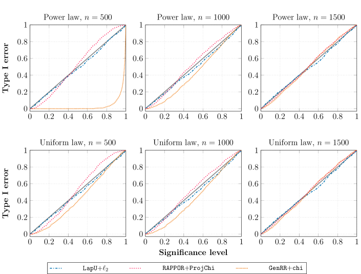
Figure 2: Comparison of type I error control between a permutation-calibrated method (LapU+$\ell_{2}$) and methods calibrated through asymptotic chi-square null distribution (RAPPOR+ProjChi and GenRR+Chi), across configurations of uniform (top row) and power-law (bottom row) null distributions as described in (17). The gray solid lines represent the $y=x$ line, indicating perfect type I error control.

Type I error control. First, we compare the type I error rates of three methods for multinomial testing: LapU+$\ell_{2}$, GenRR+Chi, and RAPPOR+ProjChi, to highlight the advantages of the permutation approach. We consider two null distributions, where for $m\in[k]$, the $m$th elements of $\mathbf{p}_{Y}$ and $\mathbf{p}_{Z}$ are defined as:

$$\text{(a) power law: }p_{{Y}{m}}=p_{{Z}{m}}\propto 1/m\quad\text{and}\quad\text{(b) uniform law: }p_{{Y}{m}}=p_{{Z}{m}}=1/k.$$ (17)

We set $k=500$ and $\alpha=0.1$, and investigate how the type I error rate varies with sample sizes $n\in\{500,1000,1500\}$. The results, displayed in Figure 2, indicate that the type I error of the permutation test, LapU+$\ell_{2}$, is well controlled at any sample size and significance level (up to a small numerical error) as expected. In contrast, we see that the asymptotic tests, namely RAPPOR+ProjChi and GenRR+Chi, have the size significantly deviated from the straight baseline, especially when the sample size is small or moderate. This indicates that the resulting asymptotic test can be either conservative or anti-conservative depending on the significance level.

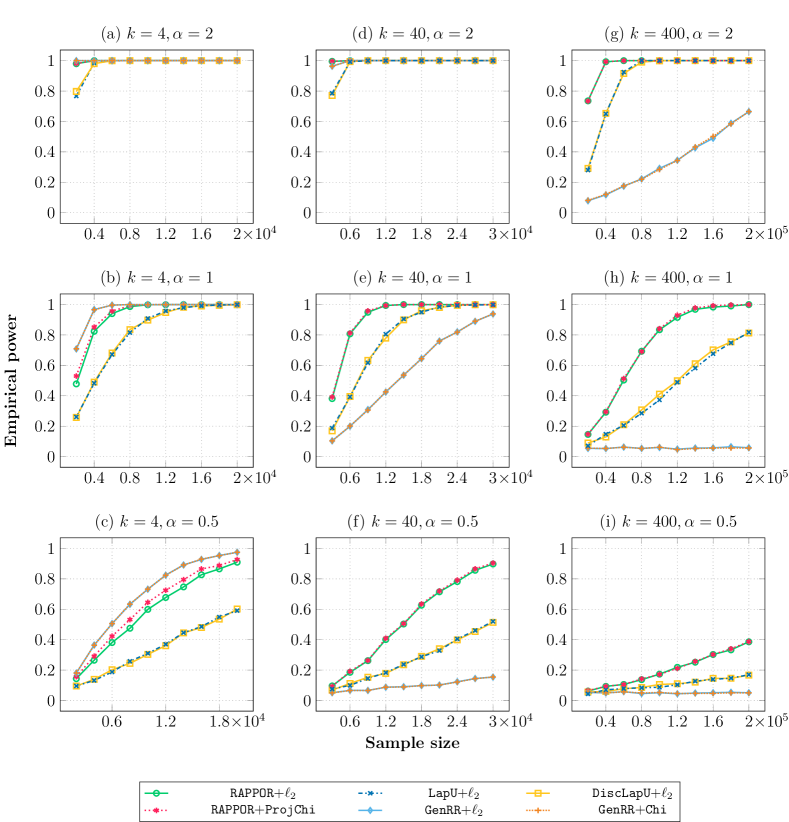
Figure 3: Comparison of the testing power between our proposed methods (first row in the legend) and baseline methods (second row in the legend) under the perturbed uniform alternatives (18). To ensure a fair comparison, all methods are calibrated using permutation procedures at level $\gamma=0.05$.

Simulation settings for power comparison in multinomial testing. We next compare the power of our proposed methods (RAPPOR+$\ell_{2}$, LapU+$\ell_{2}$, and DiscLapU+$\ell_{2}$) with baseline methods (GenRR+Chi, RAPPOR+ProjChi, and GenRR+$\ell_{2}$) for distinguishing between two multinomial distributions. As observed in Figure 2, both GenRR+Chi and RAPPOR+ProjChi can be miscalibrated when their thresholds are determined by the asymptotic null distributions. In order to ensure a fair power comparison, GenRR+Chi and RAPPOR+ProjChi were calibrated using permutation procedures in this power simulation. We aim to illustrate how the testing power varies with changes in the number of categories $k$ and the privacy parameter $\alpha$. The analysis is conducted under a perturbed uniform distribution scenario, where for $m\in[k]$, the $m$th elements of $\mathbf{p}_{Y}$ and $\mathbf{p}_{Z}$ are defined as:

$$p_{{Y}{m}}=\frac{1}{k}+(-1)^{m}\eta\leavevmode\nobreak\ \quad\text{and}\quad\leavevmode\nobreak\ p_{{Z}{m}}=\frac{1}{k}+(-1)^{(m+1)}\eta,\quad\text{for $m\in[k]$.}$$ (18)

The simulation considers the following combinations of three parameters, namely the number of categories $k$, the perturbation size $\eta$ and the privacy parameter $\alpha$:

$$(k,\eta,\alpha)\in\{(4,0.04),(40,0.015),(400,0.002)\}\times\{2,1,0.5\}.$$

The simulation results for this setting are provided in Figure 3.

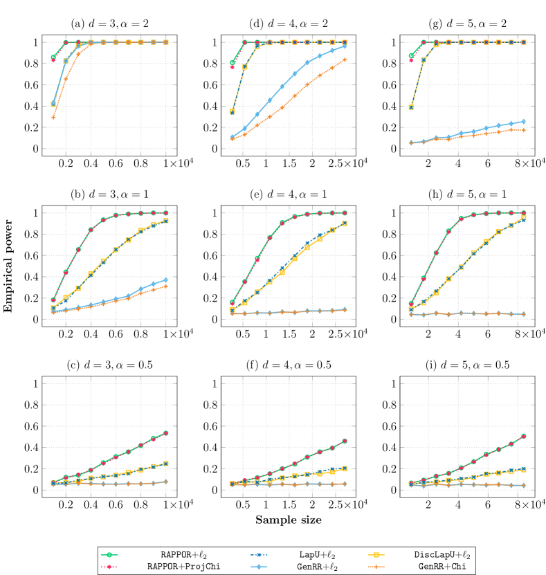
Figure 4: Comparison of the density testing power between our proposed methods (first row in the legend) and baseline methods (second row in the legend) under the location alternatives in (19). To ensure a fair comparison, all methods are calibrated using permutation procedures at level $\gamma=0.05$.

Simulation settings for power comparison in density testing. We also evaluate the density testing power of the same methods used in the simulations for multinomial testing. We consider two scenarios where two density functions differ in their location parameters or scale parameters. Since the results for scale difference show trend similar to that of location difference, we present these results in Appendix G.3. For the location difference, we analyze scenarios involving mean differences between two $d$-dimensional Gaussian distributions $P_{\mathbf{Y}}=\mathcal{N}(\bm{\mu}_{\mathbf{Y}},\Sigma_{\mathbf{Y}})$ and $P_{\mathbf{Z}}=\mathcal{N}(\bm{\mu}_{\mathbf{Z}},\Sigma_{\mathbf{Z}})$. Let $\mathbf{1}_{d}:=(1,\ldots,1)^{\top}\in\mathbb{R}^{d}$, $\mathbf{0}_{d}:=(0,\ldots,0)^{\top}\in\mathbb{R}^{d}$, $\mathbf{J}_{d}:=\mathbf{1}_{d}{\mathbf{1}_{d}}^{\top}\in\mathbb{R}^{d\times d}$, and $\mathbf{I}_{d}$ denote the identity matrix in $\mathbb{R}^{d\times d}$. We set the mean vectors and covariance matrices of the Gaussian distributions as:

$$\bm{\mu}_{\mathbf{Y}}=0.5\times\mathbf{1}_{d},\leavevmode\nobreak\ \bm{\mu}_{\mathbf{Z}}=-\bm{\mu}_{\mathbf{Y}},\quad\text{and}\quad\Sigma_{\mathbf{Y}}=\Sigma_{\mathbf{Z}}=0.5\times\mathbf{J}_{d}+0.5\times\mathbf{I}_{d}.$$ (19)

In simulations, the dimension of the original data is chosen as $d\in\{3,4,5\}$, and after binning through the map $T$ in (16) with $\kappa=4$, the number of categories becomes $k\in\{64,256,1024\}$.

Simulation results for power comparisons. The simulation results in this section are illustrated in Figures 3 and 4. We first consistently observe in all of the figures that the power tends to decrease as the privacy parameter $\alpha$ decreases meaning a stronger privacy guarantee. These trade-offs are all predictable from the minimax rates in (6) and (12). We next highlight the differences in trends related to the number of categories. For multinomial distributions with a small number of categories ($k=4$), the generalized randomized response, a natural extension of the classical mechanism (Warner,, 1965), outperforms all other methods. Following the generalized randomized response mechanism is the RAPPOR mechanism, while Laplace-noise-based mechanisms performing the least. However, in scenarios with a larger number of categories, or in density testing scenarios (which also correspond to a large number of categories), the testing power of the generalized randomized response diminishes, and RAPPOR emerges as the method with the highest power. The suboptimal performance of the generalized randomized response in high-dimensional settings, as theoretically explored in Appendix H and numerically observed by Gaboardi and Rogers, (2018), aligns with a simple intuition: since the generalized randomized response modifies data by shifting it from one category to another, the difference between the original sample and its corresponding $\alpha$-LDP view becomes more pronounced as the number of categories increases. These simulation results prove the superiority of RAPPOR over the other mechanisms, especially in multinomial testing with large $k$ and density testing, and we therefore recommend using RAPPOR in practical applications. Within the tests built upon RAPPOR, we observe in Figures 3 and 4 that RAPPOR+ProjChi and RAPPOR+$\ell_{2}$ perform comparably to each other, and in some cases, RAPPOR+ProjChi is slightly more powerful. It is also possible that the difference between RAPPOR+ProjChi and RAPPOR+$\ell_{2}$ is more pronounced in some settings. For example, if the signal is large in terms of chi-square divergence but relatively small in terms of the $\ell_{2}$ distance, we would expect RAPPOR+ProjChi to perform better than RAPPOR+$\ell_{2}$. Conversely, if the signal is large in the $\ell_{2}$ distance, the opposite holds true; we present the numerical results that confirm this in Appendix G.2. This suggests that when practitioners have insights into the nature of the deviation between two distributions, selecting a statistic that aligns with that specific deviation might be more effective. We leave it as future work to conduct more extensive simulations in diverse settings and using various types of test statistics.

6 Discussion

In this work, we studied minimax separation rates for two-sample testing under LDP constraint. Moving beyond the univariate Besov ball with $q=\infty$ considered in Lam-Weil et al., (2022), our work encompasses a larger Besov class of densities in a multivariate setting without restriction on $q$. We also considered the Hölder class and extended the non-private results of Kim et al., 2022a to a locally private setting. By noting the equivalence between the binning approach in Kim et al., 2022a and the projection approach in Lam-Weil et al., (2022), we proposed an integrated private testing framework that provides an optimal test for a large class of smooth densities. We proved our results using three distinct LDP mechanisms, thereby extending the toolkit available for practitioners. Additionally, an adaptive test is introduced that retains optimality up to a log factor without the knowledge of the smoothness parameter. Echoing prior work (Aliakbarpour et al.,, 2018, 2019; Cai et al.,, 2017; Lam-Weil et al.,, 2022), our results reaffirm that there exists an inevitable trade-off between data privacy and statistical efficiency that data analysts should bear in mind.

Our paper leaves several open questions for future investigation. Throughout the paper, we focused on equal-sized binning scheme that returns minimax optimal procedures. However, this framework may be problematic in high-dimensional settings as many bins would be empty. To address this issue, one can develop a data-adaptive binning scheme and improve the high-dimensional performance. In terms of smoothness classes, future work can be dedicated to extending our minimax result to a more general Besov class and other smoothness classes. Another interesting direction of future work is to develop optimal tests of conditional independence under privacy constraints, building on the recent work of Neykov et al., (2021) and Kim et al., 2022b . Finally, one can attempt to improve the $\log^{2}n_{1}\log\log n_{1}$ cost for adaptivity or find the matching lower bound. We leave all of these interesting but challenging problems for future work.

Appendix A Overview of Appendix

This supplementary material provides the technical proofs deferred in the main text, along with some additional results of interest. The content is organized as follows:

• Appendix B presents the technical lemmas, constructions, and calculations used in the main proofs of our results.

• Appendix C provides the proof of the $\alpha$-LDP guarantees for our proposed privacy mechanisms.

• Appendix D proves the minimax rate result for multinomial testing, as presented in Theorem 3.1.

• Appendix E proves the minimax rate result for density testing, as presented in Theorem 4.1.

• Appendix F establishes the minimax upper bound for adaptive density testing, as shown in Theorem 4.2.

• Appendix G provides additional information on the numerical studies presented in Section 5.

• Appendix H discusses the asymptotic suboptimality of the GenRR+$\ell_{2}$ multinomial test mentioned in Section 5.

Appendix B Preliminary Results

This section presents the technical lemmas, constructions, and calculations used in the main proofs.

B.1 First Two Moments of Discrete Laplace Noise

We analyze the first two moments of a discrete Laplace noise random variable to establish the upper bound for the separation rate of our private test in Theorem 3.1. The next lemma shows that the discrete noise in discrete Laplace mechanism (Definition 3.2) has mean zero and variance at most $8k/\alpha^{2}$, which matches the variance of the continuous noise in Laplace mechanism (Definition 3.1) with the same privacy guarantee.

Lemma B.1.

If $W$ follows $\mathrm{DL}(\zeta_{\alpha})$ defined in (8) and Definition 3.2, we have

$$\mathbb{E}(W)=0\quad\text{and}\quad\mathrm{Var}(W)\leq\frac{8k}{\alpha^{2}}.$$

Proof.

From Proposition 2.2 of Inusah and Kozubowski, (2006), we have $\mathbb{E}(W)=0$ and $\mathrm{Var}(W)=2\zeta_{\alpha}/(1-\zeta_{\alpha})^{2}$. Therefore, it suffices to show that

$$\frac{2\zeta_{\alpha}}{(1-\zeta_{\alpha})^{2}}\leq\frac{8k}{\alpha^{2}}.$$

For notational convenience, let $v:=\alpha/\sqrt{4k}>0$ for $\alpha>0$, so that we have $\zeta_{\alpha}=\exp({-\alpha/\sqrt{4k}})=\exp({-v}).$ The proof then reduces to showing that

$$v^{2}\leq\frac{(1-\zeta_{\alpha})^{2}}{\zeta_{\alpha}}=\bigl{(}e^{v/2}-e^{-v/2}\bigr{)}^{2}.$$

Since $v>0$, both sides of the above inequality is positive. Therefore it suffices to show that

$$v\leq e^{v/2}-e^{-v/2}.$$ (20)

Note that Taylor expansions of $\exp(v/2)$ and $\exp(-v/2)$ have the same even order terms, and their odd order terms have the same absolute values with opposite signs. Therefore, it holds that

$$(e^{v/2}-e^{-v/2})=2\cdot\sum_{n=0}^{\infty}\frac{\left(v/2\right)^{2n+1}}{(2n+1)!}=2\cdot\left((v/2)+\frac{(v/2)^{3}}{3!}+\frac{(v/2)^{5}}{5!}+\frac{(v/2)^{7}}{7!}+\cdots\right).$$

Since $v>0$, all the terms of above are positive. Thus, the condition (20) is satisfied. This concludes the proof of Lemma B.1. ∎

B.2 Summary Statistics of RAPPOR Mechanism

This section provides calculations for the summary statistics of the RAPPOR private views, which are used in Appendix D.1.2. First, Lemma B.2 presents the exact calculation of the expectation of the U-statistic in (9), as well as the variance and covariance of the entries of a RAPPOR private view.

Lemma B.2 (Summary statistics of RAPPOR private views).

Let $\{Y_{i}\}_{i\in[n_{1}]}$ be i.i.d. multinomial sample with $k$ categories. Let $\{\tilde{\mathbf{Y}}_{i}\}_{i\in[n_{1}]}$ represent the corresponding $\alpha$-LDP views obtained through the RAPPOR mechanism, where for each $m\in[k]$, the $m$th entry is distributed as

$$\tilde{Y}_{im}\sim\mathrm{Ber}\bigl{(}\alpha_{\mathrm{bf}}\mathds{1}(Y_{i}=m)+\delta_{\mathrm{bf}}\bigr{)},\leavevmode\nobreak\ \text{where}\leavevmode\nobreak\ \alpha_{\mathrm{bf}}:=\frac{e^{\alpha/2}-1}{e^{\alpha/2}+1}\quad\text{and}\quad\delta_{\mathrm{bf}}:=\frac{1}{e^{\alpha/2}+1}.$$

Then we have $\mathbb{E}[U_{n_{1},n_{2}}]=\alpha_{\mathrm{bf}}^{2}\|\mathbf{p}_{Y}-\mathbf{p}_{Z}\|_{2}^{2}$. Also, we have

$$\mathrm{Var}(\tilde{Y}_{1m})=\bigl{(}\alpha_{\mathrm{bf}}p_{{Y}{m}}+\delta_{\mathrm{bf}}\bigr{)}\bigl{(}1-\alpha_{\mathrm{bf}}p_{{Y}{m}}-\delta_{\mathrm{bf}}\bigr{)}\leavevmode\nobreak\ \text{and}\leavevmode\nobreak\ \mathrm{Cov}(\tilde{Y}_{1m},\tilde{Y}_{1m^{\prime}})=-\alpha_{\mathrm{bf}}^{2}p_{{Y}{m}}p_{{Y}{m^{\prime}}},$$

for each $m\in[k]$ and for $m,m^{\prime}\in[k]$ such that $m\neq m^{\prime}$, respectively.

Proof.

The expectation is verified as follows:

$$\mathbb{E}[U_{n_{1},n_{2}}] =\mathbb{E}[(\tilde{\mathbf{Y}}_{1}-\tilde{\mathbf{Z}}_{1})^{\top}(\tilde{\mathbf{Y}}_{2}-\tilde{\mathbf{Z}}_{2})]$$

$$=\mathbb{E}[\tilde{\mathbf{Y}}_{1}-\tilde{\mathbf{Z}}_{1}]^{\top}\mathbb{E}[\tilde{\mathbf{Y}}_{2}-\tilde{\mathbf{Z}}_{2}]$$

$$=(\alpha_{\mathrm{bf}}\;\mathbf{p}_{Y}-\alpha_{\mathrm{bf}}\mathbf{p}_{Z})^{\top}(\alpha_{\mathrm{bf}}\;\mathbf{p}_{Y}-\alpha_{\mathrm{bf}}\mathbf{p}_{Z})$$

$$=\alpha_{\mathrm{bf}}^{2}\|\mathbf{p}_{Y}-\mathbf{p}_{Z}\|_{2}^{2}.$$

The variance is verified as follows:

$$\mathrm{Var}(\tilde{Y}_{1m})=\mathbb{E}[\tilde{Y}_{1m}^{2}]-\mathbb{E}[\tilde{Y}_{1m}]^{2}\stackrel{{\scriptstyle(a)}}{{=}}\mathbb{E}[\tilde{Y}_{1m}]-\mathbb{E}[\tilde{Y}_{1m}]^{2}=\bigl{(}\alpha_{\mathrm{bf}}p_{{Y}{m}}+\delta_{\mathrm{bf}}\bigr{)}\bigl{(}1-\alpha_{\mathrm{bf}}p_{{Y}{m}}-\delta_{\mathrm{bf}}\bigr{)},$$ (21)

where step $(a)$ uses the fact that $\tilde{Y}_{1m}^{2}=\tilde{Y}_{1m}$ since $\tilde{Y}_{1m}$ is either 0 or 1. Finally, for $m,m^{\prime}\in[k]$ such that $m\neq m^{\prime}$, the covariance is calculated as:

$$\mathrm{Cov}(\tilde{Y}_{1m},\tilde{Y}_{1m^{\prime}})=\leavevmode\nobreak\ \mathbb{E}[\tilde{Y}_{1m}\tilde{Y}_{1m^{\prime}}]-\mathbb{E}[\tilde{Y}_{1m}]\mathbb{E}[\tilde{Y}_{1m^{\prime}}]$$

$$\stackrel{{\scriptstyle(a)}}{{=}}\hskip 4.4671pt \mathbb{P}[\tilde{Y}_{1m}=1,\tilde{Y}_{1m^{\prime}}=1]-\mathbb{E}[\tilde{Y}_{1m}]\mathbb{E}[\tilde{Y}_{1m^{\prime}}]$$

$$\stackrel{{\scriptstyle(b)}}{{=}}\hskip 4.60933pt \bigl{(}\alpha_{\mathrm{bf}}p_{{Y}{m}}+\delta_{\mathrm{bf}}\bigr{)}\bigl{(}\alpha_{\mathrm{bf}}p_{{Y}{m^{\prime}}}+\delta_{\mathrm{bf}}\bigr{)}-\alpha_{\mathrm{bf}}^{2}p_{{Y}{m}}p_{{Y}{m^{\prime}}}-\bigl{(}\alpha_{\mathrm{bf}}p_{{Y}{m}}+\delta_{\mathrm{bf}}\bigr{)}\bigl{(}\alpha_{\mathrm{bf}}p_{{Y}{m^{\prime}}}+\delta_{\mathrm{bf}}\bigr{)}$$

$$=\hskip 5.57675pt -\alpha_{\mathrm{bf}}^{2}p_{{Y}{m}}p_{{Y}{m^{\prime}}},$$

where step $(a)$ uses the fact that each entry is 0 or 1, and step $(b)$ is from Fact 1 of Acharya et al., (2019), which holds only when $m\neq m^{\prime}.$ ∎

We next give upper bounds for the sum of entrywise variances and covariances of an RAPPOR $\alpha$-LDP view.

Lemma B.3.

For any $m,m^{\prime}\in[k]$ such that $m^{\prime}\neq m^{\prime}$, the following inequalities hold:

$$\quad\ \sum_{m=1}^{k}\mathrm{Var}(\tilde{Y}_{1m})\bigl{(}p_{{Y}{m}}-p_{{Z}{m}}\bigr{)}^{2}\leq\alpha_{\mathrm{bf}}b^{1/2}\|\mathbf{p}_{Y}-\mathbf{p}_{Z}\|_{2}^{2}+\alpha_{\mathrm{bf}}\delta_{\mathrm{bf}}\|\mathbf{p}_{Y}-\mathbf{p}_{Z}\|_{2}^{2},$$ (22)

$$\quad\ \sum_{m=1}^{k}\mathrm{Var}(\tilde{Y}_{1m})^{2}\leq 2\alpha_{\mathrm{bf}}^{2}b+2\delta_{\mathrm{bf}}^{2}k,\leavevmode\nobreak\ \text{and}$$ (23)

$$\sum_{1\leq m\neq m^{\prime}\leq k}\mathrm{Cov}(\tilde{Y}_{1m},\tilde{Y}_{1m^{\prime}})^{2}\leq\alpha_{\mathrm{bf}}^{2}b,$$ (24)

where $b=\max\{\|\mathbf{p}_{Y}\|_{2}^{2},\|\mathbf{p}_{Z}\|_{2}^{2}\}$. The same type of inequalities also hold for $\tilde{Z}_{1m}$ and $\tilde{Z}_{1m^{\prime}}$.

Proof.

For (22), we have

$$\sum_{m=1}^{k}\mathrm{Var}(\tilde{Y}_{1m})\bigl{(}p_{{Y}{m}}-p_{{Z}{m}}\bigr{)}^{2} \stackrel{{\scriptstyle(a)}}{{=}}\sum_{m=1}^{k}\bigl{(}\alpha_{\mathrm{bf}}p_{{Y}{m}}+\delta_{\mathrm{bf}}\bigr{)}\bigl{\{}1-\bigl{(}\alpha_{\mathrm{bf}}p_{{Y}{m}}+\delta_{\mathrm{bf}}\bigr{)}\bigr{\}}\bigl{(}p_{{Y}{m}}-p_{{Z}{m}}\bigr{)}^{2}$$

$$\stackrel{{\scriptstyle(b)}}{{\leq}}\sum_{m=1}^{k}\bigl{(}\alpha_{\mathrm{bf}}p_{{Y}{m}}+\delta_{\mathrm{bf}}\bigr{)}\bigl{(}p_{{Y}{m}}-p_{{Z}{m}}\bigr{)}^{2}$$

$$\stackrel{{\scriptstyle(c)}}{{\leq}}\alpha_{\mathrm{bf}}b^{1/2}\|\mathbf{p}_{Y}-\mathbf{p}_{Z}\|_{4}^{2}+\delta_{\mathrm{bf}}\|\mathbf{p}_{Y}-\mathbf{p}_{Z}\|_{2}^{2}$$

$$\stackrel{{\scriptstyle(d)}}{{\leq}}\alpha_{\mathrm{bf}}b^{1/2}\|\mathbf{p}_{Y}-\mathbf{p}_{Z}\|_{2}^{2}+\delta_{\mathrm{bf}}\|\mathbf{p}_{Y}-\mathbf{p}_{Z}\|_{2}^{2},$$

where step $(a)$ uses Lemma B.2, step $(b)$ uses the fact that $0<\alpha_{\mathrm{bf}}p_{{Y}{m}}+\delta_{\mathrm{bf}}<1$ for any $m\in[k]$, step $(c)$ uses the Cauchy–Schwarz inequality, and step $(d)$ uses the monotonicity of the $\ell_{p}$ norm, specifically $\ell_{4}\leq\ell_{2}$.

Next, for (23), we have

$$\sum_{m=1}^{k}\mathrm{Var}(\tilde{Y}_{1m})^{2}\leq\leavevmode\nobreak\ \sum_{m=1}^{k}\bigl{(}\alpha_{\mathrm{bf}}p_{{Y}{m}}+\delta_{\mathrm{bf}}\bigr{)}^{2}\bigl{\{}1-\bigl{(}\alpha_{\mathrm{bf}}p_{{Y}{m}}+\delta_{\mathrm{bf}}\bigr{)}\bigr{\}}^{2}$$

$$\stackrel{{\scriptstyle(a)}}{{\leq}}\hskip 4.4671pt \sum_{m=1}^{k}\bigl{(}\alpha_{\mathrm{bf}}p_{{Y}{m}}+\delta_{\mathrm{bf}}\bigr{)}^{2}$$

$$\stackrel{{\scriptstyle(b)}}{{\leq}}\hskip 4.4671pt \sum_{m=1}^{k}\bigl{(}2\alpha_{\mathrm{bf}}p_{{Y}{m}}^{2}+2\delta_{\mathrm{bf}}^{2}\bigr{)}$$

$$=\hskip 5.12149pt 2\alpha_{\mathrm{bf}}^{2}\|\mathbf{p}_{Y}\|_{2}^{2}+2\delta_{\mathrm{bf}}^{2}k$$

$$\leq\hskip 4.97922pt 2\alpha_{\mathrm{bf}}^{2}b+2\delta_{\mathrm{bf}}^{2}k,$$

where step $(a)$ uses the fact that $0<\alpha_{\mathrm{bf}}p_{{Y}{m}}+\delta_{\mathrm{bf}}<1$ for any $m\in[k]$, and step $(b)$ uses the inequality $(a+b)^{2}\leq 2a^{2}+2b^{2}.$ Finally, for (24), we have

$$\sum_{1\leq m\neq m^{\prime}\leq k}\mathrm{Cov}(\tilde{Y}_{1m},\tilde{Y}_{1m^{\prime}})^{2}\stackrel{{\scriptstyle(a)}}{{=}}\hskip 4.4671pt \sum_{1\leq m\neq m^{\prime}\leq k}\alpha_{\mathrm{bf}}^{4}\;p_{{Y}{m}}^{2}p_{{Y}{m^{\prime}}}^{2}$$

$$\stackrel{{\scriptstyle(b)}}{{\leq}}\hskip 4.4671pt \alpha_{\mathrm{bf}}^{2}\sum_{m=1}^{k}p_{{Y}{m}}^{2}\sum_{m^{\prime}=1}^{k}p_{{Y}{m^{\prime}}}^{2}$$

$$=\hskip 5.03615pt \alpha_{\mathrm{bf}}^{2}\|\mathbf{p}_{Y}\|_{2}^{4}$$

$$\stackrel{{\scriptstyle(c)}}{{\leq}}\hskip 3.86957pt \alpha_{\mathrm{bf}}^{2}\|\mathbf{p}_{Y}\|_{2}^{2}$$

$$\leq\hskip 4.89388pt \alpha_{\mathrm{bf}}^{2}b,$$

where step $(a)$ uses Lemma B.2, step $(b)$ uses the fact that $0<\alpha_{\mathrm{bf}}<1$ for any $\alpha>0$, and step $(c)$ uses the fact that $\|\mathbf{p}_{Y}\|_{2}^{2}\leq 1$. ∎

B.3 Construction of Multivariate Haar Wavelet Basis

We outline the construction of multivariate Haar wavelets, following Giné and Nickl, (2015), Section 4.3.6, and Autin et al., (2010), Section 2. For $f:[0,1]\to\mathbb{R}$ and integers $u,v$, define the re-scaled and shifted version as $f_{u,v}(x):=2^{u/2}f(2^{u}x-v)$. Define the univariate Haar scaling and wavelet functions from $[0,1]$ to $\mathbb{R}$ as

$$\phi(x):=\mathds{1}(0\leq x<1)\quad\text{and}\quad\psi(x):=\mathds{1}(0\leq x<1/2)-\mathds{1}(1/2\leq x<1),$$

respectively. A multivariate Haar wavelet basis is indexed by its prime resolution level $J\in\mathbb{N}_{0}$, with each element characterized by up to three (multi) indices that range over:

1. Re-scaling: $\mathbb{N}\setminus[J-1]$,

2. Shifting: $\Lambda(j):=\{0,1,\ldots,(2^{j}-1)\}^{d}$, for an integer $j\geq J$,

3. On-off: $\mathcal{I}:=\{0,1\}^{d}\setminus\mathbf{0}$,

respectively. For any $\bm{k}=(k_{1},\ldots,k_{d})\in\Lambda(J)$, let $\phi_{J,\bm{k}}:[0,1]^{d}\to\mathbb{R}$ be a tensor product of the re-scaled and shifted $\phi$’s, evaluated at $\mathbf{x}=(x_{1},\ldots,x_{d})\in[0,1]^{d}$:

$$\phi_{J,\bm{k}}(\mathbf{x}):=\prod_{p=1}^{d}\phi_{J,k_{p}}(x_{p}).$$

For a resolution level $j\geq J$, and for any $\bm{\ell}=(\ell_{1},\ldots,\ell_{d})\in\Lambda(j)$, let $\psi_{j,\bm{\ell}}^{\mathbf{\epsilon}}:[0,1]^{d}\to\mathbb{R}$ be a mixed tensor product of re-scaled and shifted $\phi$’s and $\psi$’s, evaluated at $\mathbf{x}=(x_{1},\ldots,x_{d})\in[0,1]^{d}$:

$$\psi_{j,\bm{\ell}}^{\mathbf{\epsilon}}(\mathbf{x}):=\prod_{{p}=1}^{d}\bigl{\{}\phi_{j,\ell_{p}}(x_{p})\bigr{\}}^{1-\epsilon_{p}}\bigl{\{}\psi_{j,\ell_{p}}(x_{p})\bigr{\}}^{\epsilon_{p}}.$$

The Haar multivariate wavelet basis at prime resolution level $J$ is defined as

$$\Phi_{J}\cup\bigl{(}\bigcup_{j\geq J}\Psi_{j}\bigr{)},\text{ where }\Phi_{J}:=\{\phi_{J,\bm{k}}\}_{\bm{k}\in\Lambda(J)}\text{ and }\Psi_{j}:=\{\psi_{j,\bm{\ell}}^{\mathbf{\epsilon}}\}_{\bm{\ell}\in\Lambda(j),\mathbf{\epsilon}\in\mathcal{I}}.$$ (25)

B.4 Density Discretization Error Analysis

This section analyzes the error arising from comparing discretized multinomial probability vectors instead of the original multivariate densities. Given the number of bins $\kappa$, let ${B_{1},\dots,B_{\kappa^{d}}}$ enumerate $d$-dimensional hypercubes with side length $1/\kappa$. For a density $f_{\mathbf{Y}}$, its step function approximation is defined as:

$$\hat{f}_{\mathbf{Y}}(\mathbf{y}):=\sum_{m\in[\kappa^{d}]}\mathds{1}(\mathbf{y}\in B_{m})\kappa^{d}\int_{B_{m}}f_{\mathbf{Y}}(\mathbf{t})\;d\mathbf{t}.$$ (26)

Similarly, define $\hat{f}_{\mathbf{Z}}$ from $f_{\mathbf{Z}}$. Then it holds that $\|\mathbf{p}_{\mathbf{Y}}-\mathbf{p}_{\mathbf{Z}}\|_{2}^{2}=\kappa^{-d}|\kern-1.07639pt|\kern-1.07639pt|\hat{f}_{\mathbf{Y}}-\hat{f}_{\mathbf{Z}}|\kern-1.07639pt|\kern-1.07639pt|_{\mathbb{L}_{2}}^{2}$. We analyze the differenece between $|\kern-1.07639pt|\kern-1.07639pt|\hat{f}_{\mathbf{Y}}-\hat{f}_{\mathbf{Z}}|\kern-1.07639pt|\kern-1.07639pt|_{\mathbb{L}_{2}}$ and $|\kern-1.07639pt|\kern-1.07639pt|f_{\mathbf{Y}}-f_{\mathbf{Z}}|\kern-1.07639pt|\kern-1.07639pt|_{\mathbb{L}_{2}}$ when $(f_{\mathbf{Y}}-f_{\mathbf{Z}})$ lies in $\mathcal{B}_{d,s}^{\mathrm{H}}(R)$ or $\mathcal{B}_{d,s,\infty}^{\mathrm{B}}(R)$. For both cases, the discretization error scales as $\kappa^{-s}$, where we recall that $s$ is the smoothness parameter. For the Hölder density case, the analysis is a simple application of Lemma 7.2 of Arias-Castro et al., (2018), rephrased below:

Lemma B.4.

For a function $h\in\mathcal{B}_{d,s}^{\mathrm{H}}(R)$, let $\hat{h}$ be its step function approximation as in (26), with $\kappa$ bins. Then there exist positive constants $C_{1}$ and $C_{2}$ depending only on $d,s$ and $R$, but not on $h$, such that

$$|\kern-1.07639pt|\kern-1.07639pt|\hat{h}_{\kappa}|\kern-1.07639pt|\kern-1.07639pt|_{\mathbb{L}_{2}}\geq C_{1}{\left|\kern-1.07639pt\left|\kern-1.07639pt\left|h\right|\kern-1.07639pt\right|\kern-1.07639pt\right|}_{\mathbb{L}_{2}}-C_{2}\kappa^{-s}.$$

Substituting $(f_{\mathbf{Y}}-f_{\mathbf{Z}})\in\mathcal{B}_{d,s}^{\mathrm{H}}(R)$ into $h$ in Lemma B.4, the discretization error is characterized as follows:

$$\|\mathbf{p}_{\mathbf{Y}}-\mathbf{p}_{\mathbf{Z}}\|_{2}\geq\kappa^{-d/2}\bigl{(}C_{1}|\kern-1.07639pt|\kern-1.07639pt|f_{\mathbf{Y}}-f_{\mathbf{Z}}|\kern-1.07639pt|\kern-1.07639pt|_{\mathbb{L}_{2}}-C_{2}\kappa^{-s}\bigr{)}.$$ (27)

For the Besov density case, we derive a similar lemma as follows:

Lemma B.5.

Define $\mathcal{B}_{d,s,\infty}^{\mathrm{B}}(R)$ using Haar multivariate wavelet basis at prime resolution level $J$ constructed in Appendix B.3. For a function $(f_{\mathbf{Y}}-f_{\mathbf{Z}})\in\mathcal{B}_{d,s,\infty}^{\mathrm{B}}(R)$, the following error bound holds:

$$\|\mathbf{p}_{\mathbf{Y}}-\mathbf{p}_{\mathbf{Z}}\|_{2}\geq\kappa^{-d/2}\bigl{(}|\kern-1.07639pt|\kern-1.07639pt|f_{\mathbf{Y}}-f_{\mathbf{Z}}|\kern-1.07639pt|\kern-1.07639pt|_{\mathbb{L}_{2}}-R\kappa^{-s}\bigr{)},$$ (28)

where $\kappa=2^{J}$ and $\mathbf{p}_{\mathbf{Y}}$ and $\mathbf{p}_{\mathbf{Z}}$ are binned with side length $1/\kappa$.

Proof.

Let $\Phi_{J}\cup(\bigcup_{j\geq J}\Psi_{j})$ denote the Haar multivariate wavelet basis that defines $\mathcal{B}_{d,s,\infty}^{\mathrm{B}}(R)$. The analysis proceeds in two steps. First, we show that the sum of squared coefficients from projecting $(f_{\mathbf{Y}}-f_{\mathbf{Z}})$ onto span($\Phi_{J}$) equals the scaled $\ell_{2}$ distance between the probability vectors:

$$\sum_{\phi\in\Phi_{J}}\theta^{2}_{\phi}(f_{\mathbf{Y}}-f_{\mathbf{Z}})=\leavevmode\nobreak\ \sum_{(k_{1},\ldots k_{d})\in\Lambda(J)}\left(\int_{[0,1]^{d}}\bigl{(}f_{\mathbf{Y}}(\mathbf{x})-f_{\mathbf{Z}}(\mathbf{x})\bigr{)}\prod_{p=1}^{d}\phi_{J,k_{p}}(x_{p})\;d\mathbf{x}\right)^{2}$$

$$\stackrel{{\scriptstyle(a)}}{{=}}\hskip 4.4671pt \kappa^{d}\sum_{(k_{1},\ldots k_{d})\in\Lambda(J)}\left(\int_{[0,1]^{d}}\bigl{(}f_{\mathbf{Y}}(\mathbf{x})-f_{\mathbf{Z}}(\mathbf{x})\bigr{)}\prod_{p=1}^{d}\mathds{1}\biggl{(}\frac{k_{p}}{\kappa}\leq x_{p}<\frac{k_{p}+1}{\kappa}\biggr{)}\;d\mathbf{x}\right)^{2}$$

$$=\leavevmode\nobreak\ \kappa^{d}\sum_{m\in[\kappa^{d}]}\left(\int_{B_{m}}\bigl{(}f_{\mathbf{Y}}(\mathbf{x})-f_{\mathbf{Z}}(\mathbf{x})\bigr{)}\;d\mathbf{x}\right)^{2}$$

$$=\leavevmode\nobreak\ \kappa^{d}\|\mathbf{p}_{Y}-\mathbf{p}_{Z}\|_{2}^{2},$$ (29)

where step $(a)$ uses the definition $\phi_{J,\bm{k}}(\mathbf{x})=\prod_{p=1}^{d}\phi_{J,k_{p}}(x_{p})$, with $\phi:[0,1]\to\{0,1\}$ defined as $\phi(x)=\mathds{1}(0\leq x<1)$, and $\phi_{J,k_{p}}(x_{p})=2^{J/2}f(2^{J}x_{p}-k_{p})$ indicates its re-scaled and shifted version. See Appendix B.3 for details. Since ${\Phi}_{J}\cup\bigl{(}\bigcup_{j\geq J}{\Psi}_{j}\bigr{)}$ forms an orthonormal basis of $\mathbb{L}_{2}([0,1]^{{d}})$, the approximation error is given by the sum of squared projection coefficients of $(f_{\mathbf{Y}}-f_{\mathbf{Z}})$ onto $\text{span}\bigl{(}\bigcup_{j\geq J}\Psi_{j}\bigr{)}$. Bounding this term is the second step of our analysis, which begins by noting that from Definition 4.2, for any $j\in\mathbb{N}_{0}$, the sum of squared wavelet coefficients is bounded as

$$\sum_{\psi\in{\Psi}_{j}}\theta_{\psi}^{2}(f_{\mathbf{Y}}-f_{\mathbf{Z}})\leq 2^{-2js}R^{2}.$$ (30)

Then the approximation error is bounded as follows:

$$|\kern-1.07639pt|\kern-1.07639pt|f_{\mathbf{Y}}-f_{\mathbf{Z}}|\kern-1.07639pt|\kern-1.07639pt|_{\mathbb{L}_{2}}^{2}-\kappa^{d}\|\mathbf{p}_{Y}-\mathbf{p}_{Z}\|_{2}^{2} =\sum_{j=J}^{\infty}\sum_{\psi\in{\Psi}_{j}}\theta_{\psi}^{2}(f_{\mathbf{Y}}-f_{\mathbf{Z}})$$

$$\stackrel{{\scriptstyle(a)}}{{\leq}}\sum_{j=J}^{\infty}2^{-2js}R^{2}$$

$$\stackrel{{\scriptstyle(b)}}{{=}}R^{2}\frac{2^{-2Js}}{1-2^{-2s}}\leq R^{2}2^{-2Js}=R^{2}\kappa^{-2s},$$

where step $(a)$ uses (30), and step $(b)$ uses an infinite geometric series. Applying $\sqrt{x+y}\leq\sqrt{x}+\sqrt{y}$ to the inequality above, we get

$$|\kern-1.07639pt|\kern-1.07639pt|f_{\mathbf{Y}}-f_{\mathbf{Z}}|\kern-1.07639pt|\kern-1.07639pt|_{\mathbb{L}_{2}}=\kappa^{d/2}\|\mathbf{p}_{Y}-\mathbf{p}_{Z}\|_{2}+R2^{-Js}\kappa^{d/2}\|\mathbf{p}_{Y}-\mathbf{p}_{Z}\|_{2}+R\kappa^{-s}.$$

∎

B.5 Gaussian Approximation of One-Sample U-statistic

The theorems presented here are used to establish a negative result for our statistic in (9) when applied with the generalized randomized response mechanism. First, Theorem B.1 restates a result from Kim, (2020), which demonstrates the asymptotic normality of a one-sample U-statistic, which is a special case of our statistic in (9) with either $n_{1}=\infty$ or $n_{2}=\infty$ under the uniform null hypothesis.

Theorem B.1 (Kim,, 2020, Corollary 3.3).

Consider a multinomial goodness-of-fit test where the null hypothesis is a discrete uniform distribution with $k$ categories, whose probability vector is denoted as $\bm{\pi}_{0}$. Let $\{\mathbf{Y}_{i}\}_{i=1}^{n}$ be a random sample represented in one-hot vector form drawn from $\bm{\pi}_{0}$. Define the U-statistic as:

$$U_{I}:={\binom{n}{2}}^{-1}\sum_{1\leq i<j\leq n}(\mathbf{Y}_{i}-\bm{\pi}_{0})^{\top}(\mathbf{Y}_{j}-\bm{\pi}_{0}).$$ (31)

If $n/\sqrt{k}\to\infty$, then the test statistic $U_{I}$ has the following asymptotic normality:

$$\sqrt{\binom{n}{2}}\frac{U_{I}}{\sqrt{(1-1/k)/k}}\overset{d}{\longrightarrow}\mathcal{N}(0,1).$$

The next theorem studies the limiting distribution of $U_{I}$ under the alternative hypothesis.

Theorem B.2 (Kim,, 2020, Theorem 3.3).

Consider the same testing problem as Theorem B.1. Let $\Sigma:=\mathrm{Cov}(\mathbf{Y}_{1})$. Under the alternative where the data is generated from a multinomial distribution with a probability vector $\bm{\pi}\neq\bm{\pi}_{0}$, suppose that the following conditions hold as $n,k\to\infty$:

1. $\dfrac{\mathrm{tr}(\Sigma^{4})}{\bigl{\{}\mathrm{tr}(\Sigma^{2})\bigr{\}}^{2}}\to 0.$

2. $\dfrac{\mathbb{E}[\bigl{\{}(\mathbf{Y}_{1}-\bm{\pi}_{0})^{\top}(\mathbf{Y}_{2}-\bm{\pi}_{0})\bigr{\}}^{4}]+n_{1}\mathbb{E}[\bigl{\{}(\mathbf{Y}_{1}-\mathbf{p}_{Z})^{\top}(\mathbf{Y}_{2}-\mathbf{p}_{Z}\bigr{\}}^{2}\bigl{\{}(\mathbf{Y}_{1}-\mathbf{p}_{Z})^{\top}(\mathbf{Y}_{3}-\mathbf{p}_{Z})\bigr{\}}^{2}]}{n^{2}\left\{\mathrm{tr}(\Sigma^{2})\right\}^{2}}\to 0.$

3. $(\bm{\pi}-\bm{\pi}_{0})^{\top}\Sigma(\bm{\pi}-\bm{\pi}_{0})<\infty$.

Then the test statistic $U_{I}$ in (31) has the following asymptotic normality:

$$\sqrt{\frac{n(n-1)}{2}}\frac{U_{I}-\|\bm{\pi}-\bm{\pi}_{0}\|_{2}^{2}}{\sqrt{\mathrm{tr}(\Sigma^{2})+2(n-1)(\bm{\pi}-\bm{\pi}_{0})^{\top}\Sigma(\bm{\pi}-\bm{\pi}_{0})}}\stackrel{{\scriptstyle d}}{{\to}}\mathcal{N}(0,1).$$ (32)

Appendix C Proof of Lemma 3.1

This section provides privacy guarantee proof for the mechanisms proposed in Section 3.2. The privacy proof for the RAPPOR mechanism is given in Section 3.2 of Duchi et al., (2013). The privacy proof for the Laplace mechanism is a minor modification of the proof of Lemma 4.2 from Lam-Weil et al., (2022), adjusting the domain of the raw samples. Thus, we only present the privacy proof for the discrete Laplace mechanism, defined in Definition 3.2. Its outline resembles the proof of Lemma 4.2 from Lam-Weil et al., (2022).

Proof.

We note that the conditional distribution of the $m$th entry of its $\alpha$-LDP view, denoted as $\tilde{X}_{im}$, is a discrete Laplace distribution with parameter $\zeta_{\alpha}=\exp({-\alpha/(2\sqrt{k}}))$, shifted by $\sqrt{k}\mathds{1}(X_{i}=m)$. Note again that for $m\neq m^{\prime}$, $\tilde{X}_{im}$ and $\tilde{X}_{im^{\prime}}$ are independent. With slight abuse of notation, we denote the conditional density function of $\tilde{\mathbf{X}}_{i}$ as $q_{i}(\cdot\,|\,\cdot)$, which can be written as

$$q_{i}(\tilde{\mathbf{x}}\,|\,x)=\prod_{m=1}^{k}\frac{1-\zeta_{\alpha}}{1+\zeta_{\alpha}}\zeta_{\alpha}^{|\tilde{x}_{m}-\sqrt{k}\mathds{1}(x=m)|}.$$

Then for all $\tilde{\mathbf{x}}=(\tilde{\mathbf{x}}_{1},\ldots,\tilde{\mathbf{x}}_{k})^{\top}\in\mathbb{R}^{k}$ and all $x,x^{\prime}\in[k]$, we have

$$\frac{q_{i}(\tilde{\mathbf{x}}\,|\,x)}{q_{i}(\tilde{\mathbf{x}}\,|\,x^{\prime})}\leavevmode\nobreak\ =\leavevmode\nobreak\ \prod_{m=1}^{k}\zeta_{\alpha}^{|\tilde{x}_{m}-\sqrt{k}\mathds{1}(x=m)|-|\tilde{x}_{m}-\sqrt{k}\mathds{1}(x^{\prime}=m)|}$$

$$=\leavevmode\nobreak\ \zeta_{\alpha}^{\sum_{m=1}^{k}|\tilde{x}_{m}-\sqrt{k}\mathds{1}(x=m)|-|\tilde{x}_{m}-\sqrt{k}\mathds{1}(x^{\prime}=m)|}$$

$$\stackrel{{\scriptstyle(a)}}{{\leq}}\hskip 4.4671pt \bigl{(}\zeta_{\alpha}^{-1}\bigr{)}^{\sum_{m=1}^{k}\bigl{|}|\tilde{x}_{m}-\sqrt{k}\mathds{1}(x=m)|-|\tilde{x}_{m}-\sqrt{k}\mathds{1}(x^{\prime}=m)|\bigr{|}}$$

$$\stackrel{{\scriptstyle(b)}}{{\leq}}\hskip 4.4671pt \bigl{(}\zeta_{\alpha}^{-1}\bigr{)}^{\sum_{m=1}^{k}\bigl{\{}\sqrt{k}\mathds{1}(x=m)+\sqrt{k}\mathds{1}(x^{\prime}=m)\bigr{\}}}$$

$$\stackrel{{\scriptstyle(c)}}{{\leq}}\hskip 4.4671pt \bigl{(}\zeta_{\alpha}^{-1}\bigr{)}^{2\sqrt{k}}=e^{\alpha},$$

where step $(a)$ uses the fact that $\zeta_{\alpha}^{x}\leq\zeta_{\alpha}^{-|x|}$ for all $x\in\mathbb{R}$ since $\zeta_{\alpha}\in(0,1)$, step $(b)$ uses the reverse triangle inequality, and step $(c)$ holds since $\mathds{1}(x=m)\neq 0$ for only a single value of $m$. Using the inequality above, for any Borel set $A\in\mathcal{B}(\mathbb{R}^{d})$, and for any $x,x^{\prime}\in[k]$, we have:

$$\frac{Q_{i}(A\,|\,x)}{Q_{i}(A\,|\,x^{\prime})}=\frac{\int_{A}q_{i}(\tilde{\mathbf{x}}\,|\,x)\,d\tilde{\mathbf{x}}}{\int_{A}q_{i}(\tilde{\mathbf{x}}\,|\,x^{\prime})\,d\tilde{\mathbf{x}}}\leq\frac{\int_{A}q_{i}(\tilde{\mathbf{x}}\,|\,x^{\prime})e^{\alpha}\,d\tilde{\mathbf{x}}}{\int_{A}q_{i}(\tilde{\mathbf{x}}\,|\,x)e^{-\alpha}\,d\tilde{\mathbf{x}}}=\frac{Q_{i}(A\,|\,x^{\prime})}{Q_{i}(A\,|\,x)}e^{2\alpha}.$$

This completes the proof of the guarantee for the discrete Laplace mechanism. ∎

Appendix D Proof of Theorem 3.1

In this section, we prove the minimax rate result for multinomial testing presented in Theorem 3.1, first focusing on the upper bound result followed by the lower bound result.

D.1 Upper Bound

This section demonstrates that the permutation test with the U-statistic proposed in (9), in conjunction with one of the mechanisms $\{\texttt{LapU},\texttt{DiscLapU},\texttt{RAPPOR}\}$, achieves a tight upper bound presented in Theorem 3.1. Since the permutation procedure controls the type I error, it suffices to prove that the condition in Theorem 3.1 guarantees type II error control. Let

$$b:=\max\{\|\mathbf{p}_{Y}\|_{2}^{2},\|\mathbf{p}_{Z}\|_{2}^{2}\}.$$ (33)

The control of the type II error is then rephrased in the following lemma.

Lemma D.1.

Assume the settings of Theorem 3.1. For each of the mechanisms $\{\textnormal{{LapU}},\textnormal{{DiscLapU}},\textnormal{{RAPPOR}}\}$, there exists a constant $C_{u}(\gamma,\beta)$ such that the type II error of the permutation test of size $\gamma$ with U-statistic in (9) is uniformly controlled by $\beta$ over $\mathcal{P}_{1,\mathrm{multi}}$ if

$$\rho_{n_{1},n_{2}}\geq C_{u}(\gamma,\beta)\left(\frac{k^{1/4}}{(n_{1}\alpha^{2})^{1/2}}\vee\frac{{b}^{1/4}}{n_{1}^{1/2}}\right).$$ (34)

Since ${b}\leq 1$, Lemma D.1 proves the upper bound result of Theorem 3.1. To prove Lemma D.1, we leverage the two moments method (Theorem 4.1 of Kim et al., 2022a, ), rephrased in Lemma D.2. This method states that if the test statistic’s expectation is sufficiently larger than a variance proxy, then uniform type II error control is achieved for the permutation test with a two-sample U-statistic of order 2. Its key advantage is that the condition bypasses the randomness arising from permutations. It lets us avoid the complex analysis typically required for permuted statistics.

To proceed, consider the following kernel:

$$h_{ts}(\mathbf{y}_{1},\mathbf{y}_{2};\mathbf{z}_{1},\mathbf{z}_{2})=\mathbf{y}_{1}^{\top}\mathbf{y}_{2}+\mathbf{z}_{1}^{\top}\mathbf{z}_{2}-\mathbf{z}_{1}^{\top}\mathbf{y}_{2}-\mathbf{z}_{2}^{\top}\mathbf{y}_{1},$$ (35)

which defines our two-sample U-statistic $U_{n_{1},n_{2}}$ in (9). Its symmetrized version, denoted $h_{ts}$, is defined as:

$$\check{h}_{ts}(\mathbf{y}_{1},\mathbf{y}_{2};\mathbf{z}_{1},\mathbf{z}_{2}):=\frac{1}{2!2!}\sum_{1\leq i_{1}\neq i_{2}\leq n_{1}}\sum_{1\leq j_{1}\neq j_{2}\leq n_{2}}h_{ts}(\mathbf{y}_{i_{1}},\mathbf{y}_{i_{2}};\mathbf{z}_{j_{1}},\mathbf{z}_{j_{2}}).$$

For the upper bound analysis, we use a U-statistic represented by $\check{h}_{ts}$, which is equivalent to our original statistic in $U_{n_{1},n_{2}}$ (9). Recall that under the LDP constraint, the raw samples $\{{Y}_{i}\}_{i\in[n_{1}]}$ and $\{{Z}_{j}\}_{j\in[n_{2}]}$ are generated from $P=(P_{Y},P_{Z})$ and then transformed into LDP-views $\{{\tilde{\mathbf{Y}}}_{i}\}_{i\in[n_{1}]}$ and $\{{\tilde{\mathbf{Z}}}_{j}\}_{j\in[n_{2}]}$ through an LDP mechanism $Q$. Let us denote the associated moments as

$$M_{Y,1}(P,Q) :=\mathrm{Var}_{P,Q}[\mathbb{E}\{\check{h}_{ts}(\tilde{\mathbf{Y}}_{1},\tilde{\mathbf{Y}}_{2};\tilde{\mathbf{Z}}_{1},\tilde{\mathbf{Z}}_{2})\,|\,\tilde{\mathbf{Y}}_{1}\}],$$

$$M_{Z,1}(P,Q) :=\mathrm{Var}_{P,Q}[\mathbb{E}\{\check{h}_{ts}(\tilde{\mathbf{Y}}_{1},\tilde{\mathbf{Y}}_{2};\tilde{\mathbf{Z}}_{1},\tilde{\mathbf{Z}}_{2})\,|\,\tilde{\mathbf{Z}}_{1}\}],$$

$$M_{YZ,2}(P,Q) :=\max\{\mathbb{E}[(\tilde{\mathbf{Y}}_{1}^{\top}\tilde{\mathbf{Y}}_{2})^{2}],\,\mathbb{E}[(\tilde{\mathbf{Y}}_{1}^{\top}\tilde{\mathbf{Z}}_{1})^{2}],\,\mathbb{E}[(\tilde{\mathbf{Z}}_{1}^{\top}\tilde{\mathbf{Z}}_{2})^{2}]\}.$$ (36)

Using these moments, we rephrase the two moments method under the setting of LDP.

Lemma D.2 (Two moments method).

Let $U_{n_{1},n_{2}}$ be a two-sample U-statistic based on the kernel given in (35). Assume that the samples are privatized through an $\alpha$-LDP mechanism $Q$. Then there exists a sufficiently large constant $C>0$ such that if

$$\mathbb{E}[U_{n_{1},n_{2}}]\geq C\sqrt{\max\left\{\frac{M_{Y,1}(P,Q)}{\beta n_{1}},\frac{M_{Z,1}(P,Q)}{\beta n_{2}},\frac{M_{YZ,2}(P,Q)}{\gamma\beta}\left(\frac{1}{n_{1}}+\frac{1}{n_{2}}\right)^{2}\right\}}$$ (37)

for all pairs of distributions $P=(P_{Y},P_{Z})\in\mathcal{P}_{1,\mathrm{multi}}(\rho_{n_{1},n_{2}})$, then the type II error of the permutation test over $\mathcal{P}_{1,\mathrm{multi}}(\rho_{n_{1},n_{2}})$ is uniformly bounded by $\beta$ as in (LABEL:eq:uniform_control).

Having stated the two moments method, our goal is to verify that inequality (37) holds under the separation conditions described in Section 3.2. We provide separate proofs for the Laplace-noise based mechanisms (LapU and DiscLapU) and the RAPPOR mechanism. However, both proofs follow the same two steps:

1. Derive upper bounds for the moments $M_{Y,1}(P,Q),M_{Z,1}(P,Q)$, and $M_{YZ,2}(P,Q)$ in (36).

2. Using the upper bounds established in Step 1, show that condition (37) in the two moments method is fulfilled as long as inequality (34) in Lemma D.1 holds.

We now verify the previous preliminary steps in order, first assuming the Laplace-noise based mechanisms.

D.1.1 Proof of Lemma D.1 Through Laplace or Discrete Laplace Mechanism

Since the analysis for Laplace and discrete Laplace mechanism is similar, we present the proof using the former (see Remark D.1 for details).

Proof.

We follow the two steps mentioned above.

Step 1: Bound the moments from above. We start by bounding the variance of conditional expectation terms. Recall the notation $M_{Y,1}(P,Q)=\mathrm{Var}_{P,Q}[\mathbb{E}\{\check{h}_{ts}(\tilde{\mathbf{Y}}_{1},\tilde{\mathbf{Y}}_{2};\tilde{\mathbf{Z}}_{1},\tilde{\mathbf{Z}}_{2})\,|\,\tilde{\mathbf{Y}}_{1}\}]$. To upper bound $M_{Y,1}(P,Q)$, we first calculate the conditional expectation of the kernel function, namely $A:=\mathbb{E}\{\check{h}_{ts}(\tilde{\mathbf{Y}}_{1},\tilde{\mathbf{Y}}_{2};\tilde{\mathbf{Z}}_{1},\tilde{\mathbf{Z}}_{2})\,|\,\tilde{\mathbf{Y}}_{1}\}$. Then we bound the variance of $A$.

For the conditional expectation, recall the $m$th component of $\mathbf{p}_{Y},\mathbf{p}_{Z},\tilde{\mathbf{Y}}_{i},\tilde{\mathbf{Z}}_{j}$ are denoted as $p_{{Y}{m}},p_{{Z}{m}},\tilde{Y}_{im}$ and $\tilde{Z}_{j,m}$, respectively. Due to i.i.d. assumptions, regardless of privacy mechanism, we have the following equalities and inequalities. First we calculate the conditional expectation:

$$A :=\mathbb{E}\bigl{[}\check{h}_{ts}(\tilde{\mathbf{Y}}_{1},\tilde{\mathbf{Y}}_{2};\tilde{\mathbf{Z}}_{1},\tilde{\mathbf{Z}}_{2})\,|\,\tilde{\mathbf{Y}}_{1}\bigr{]}=\bigl{(}\tilde{\mathbf{Y}}_{1}-\mathbb{E}[\tilde{\mathbf{Z}}_{1}]\bigr{)}^{\top}\bigl{(}\mathbb{E}[\tilde{\mathbf{Y}}_{1}]-\mathbb{E}[\tilde{\mathbf{Z}}_{1}]\bigr{)}.$$

Then we calculate the unconditional expectation:

$$\mathbb{E}[A]=\bigl{(}\mathbb{E}[\tilde{\mathbf{Y}}_{1}]-\mathbb{E}[\tilde{\mathbf{Z}}_{1}]\bigr{)}^{\top}\bigl{(}\mathbb{E}[\tilde{\mathbf{Y}}_{1}]-\mathbb{E}[\tilde{\mathbf{Z}}_{1}]\bigr{)}=\|\mathbb{E}[\tilde{\mathbf{Y}}_{1}]-\mathbb{E}[\tilde{\mathbf{Z}}_{1}]\|_{2}^{2}.$$

Then the squared and centered conditional expectation is calculated as follows:

$$A-\mathbb{E}[A] =\bigl{(}\tilde{\mathbf{Y}}_{1}-\mathbb{E}[\tilde{\mathbf{Y}}_{1}]\bigr{)}^{\top}\bigl{(}\mathbb{E}[\tilde{\mathbf{Y}}_{1}]-\mathbb{E}[\tilde{\mathbf{Z}}_{1}]\bigr{)}.$$

Based on this, the variance is calculated as

$$\mathbb{E}\bigl{[}\bigl{(}A-\mathbb{E}[A]\bigr{)}^{2}\bigr{]}=\leavevmode\nobreak\ \mathbb{E}\bigl{[}\bigl{\{}\bigl{(}\tilde{\mathbf{Y}}_{1}-\mathbb{E}[\tilde{\mathbf{Y}}_{1}]\bigr{)}^{\top}\bigl{(}\mathbb{E}[\tilde{\mathbf{Y}}_{1}]-\mathbb{E}[\tilde{\mathbf{Z}}_{1}]\bigr{)}\bigr{\}}^{2}\bigr{]}$$ (38)

$$=\leavevmode\nobreak\ \mathbb{E}\bigl{[}\bigl{\{}\tilde{\mathbf{Y}}_{1}^{\top}\bigl{(}\mathbb{E}[\tilde{\mathbf{Y}}_{1}]-\mathbb{E}[\tilde{\mathbf{Z}}_{1}]\bigr{)}-\mathbb{E}[\tilde{\mathbf{Y}}_{1}]^{\top}\bigl{(}\mathbb{E}[\tilde{\mathbf{Y}}_{1}]-\mathbb{E}[\tilde{\mathbf{Z}}_{1}]\bigr{)}\bigr{\}}^{2}\bigr{]}$$

$$\leq\leavevmode\nobreak\ 2\mathbb{E}\bigl{[}\bigl{\{}\tilde{\mathbf{Y}}_{1}^{\top}\bigl{(}\mathbb{E}[\tilde{\mathbf{Y}}_{1}]-\mathbb{E}[\tilde{\mathbf{Z}}_{1}]\bigr{)}\bigr{\}}^{2}\bigr{]}+2\bigl{[}\bigl{\{}\mathbb{E}[\tilde{\mathbf{Y}}_{1}]^{\top}\bigl{(}\mathbb{E}[\tilde{\mathbf{Y}}_{1}]-\mathbb{E}[\tilde{\mathbf{Z}}_{1}]\bigr{)}\bigr{\}}^{2}\bigr{]},$$ (39)

where the last inequality uses $(x+y)^{2}\leq 2x^{2}+2y^{2}$. Using $\|\mathbf{p}_{Y}\|_{2}\leq 1$, we bound the second term in (39) by

$$2k^{2}\|\mathbf{p}_{Y}\|_{2}\|\mathbf{p}_{Y}-\mathbf{p}_{Z}\|_{2}^{2}.$$ (40)

For the first term, we leverage the structure of our privacy mechanism, which adds independent and centered noises. Applying the Cauchy–Schwarz inequality then provides an upper bound, reducing the order of $k$ compared to a direct application of Cauchy–Schwarz. More formally,

$$2\mathbb{E}\Bigl{\{}\tilde{\mathbf{Y}}_{1}^{\top} \bigl{(}\mathbb{E}[\tilde{\mathbf{Y}}_{1}]-\mathbb{E}[\tilde{\mathbf{Z}}_{1}]\bigr{)}\Bigr{\}}^{2}$$

$$=\leavevmode\nobreak\ 2\sum_{m=1}^{k}\sum_{m^{\prime}=1}^{k}\mathbb{E}[\tilde{Y}_{1m}\tilde{Y}_{1m^{\prime}}]\bigl{(}\mathbb{E}[\tilde{Y}_{1m}]-\mathbb{E}[\tilde{Z}_{1m}]\bigr{)}\bigl{(}\mathbb{E}[\tilde{Y}_{1m^{\prime}}]-\mathbb{E}[\tilde{Z}_{1m^{\prime}}]\bigr{)}$$

$$\stackrel{{\scriptstyle(a)}}{{=}}\hskip 4.4671pt 2\sum_{m=1}^{k}\mathbb{E}[\tilde{Y}_{1m}^{2}]\bigl{(}\mathbb{E}[\tilde{Y}_{1m}]-\mathbb{E}[\tilde{Z}_{1m}]\bigr{)}^{2}$$

$$\stackrel{{\scriptstyle(b)}}{{=}}\hskip 4.4671pt 2\sum_{m=1}^{k}\bigl{\{}kp_{{Y}{m}}+\sigma_{\alpha}^{2}\bigr{\}}\bigl{(}\mathbb{E}[\tilde{Y}_{1m}]-\mathbb{E}[\tilde{Z}_{1m}]\bigr{)}^{2}$$

$$=\leavevmode\nobreak\ 2\sum_{m=1}^{k}kp_{{Y}{m}}\bigl{(}\mathbb{E}[\tilde{Y}_{1m}]-\mathbb{E}[\tilde{Z}_{1m}]\bigr{)}^{2}+2k\sigma_{\alpha}^{2}\|\mathbf{p}_{Y}-\mathbf{p}_{Z}\|_{2}^{2}$$

$$\stackrel{{\scriptstyle(c)}}{{\leq}}\hskip 4.4671pt 2k^{2}\|\mathbf{p}_{Y}\|_{2}\|\mathbf{p}_{Y}-\mathbf{p}_{Z}\|_{2}^{2}+2k\sigma_{\alpha}^{2}\|\mathbf{p}_{Y}-\mathbf{p}_{Z}\|_{2}^{2},$$ (41)

where step $(a)$ uses $\mathbb{E}[\tilde{Y}_{1m}\tilde{Y}_{1m^{\prime}}]=0$ for $m\neq m^{\prime}$, step $(b)$ uses $\mathbb{E}[\tilde{Y}_{1m}^{2}]=kp_{{Y}{m}}+\sigma_{\alpha}^{2}$, and step $(c)$ uses the Cauchy–Schwarz inequality, $\|\mathbf{p}_{Y}\|_{2}^{2}\leq\|\mathbf{p}_{Y}\|_{2}$, and monotonicity of $\ell_{p}$ norm, specifically $\ell_{4}\leq\ell_{2}$. Combining the results in (40) and (41), we achieve an upper bound for $M_{Y,1}(P,Q)$ given as

$$M_{Y,1}(P,Q)\leq\bigl{(}4k^{2}\|\mathbf{p}_{Y}\|_{2}+2k\sigma_{\alpha}^{2}\bigr{)}\|\mathbf{p}_{Y}-\mathbf{p}_{Z}\|_{2}^{2}.$$ (42)

By symmetry, we also have

$$M_{Z,1}(P,Q)\leq\bigl{(}4k^{2}\|\mathbf{p}_{Z}\|_{2}+2k\sigma_{\alpha}^{2}\bigr{)}\|\mathbf{p}_{Y}-\mathbf{p}_{Z}\|_{2}^{2}.$$ (43)

Combining the upper bound results of (42) and (43), and keeping in mind that ${b}=\max\{\|\mathbf{p}_{Y}\|_{2}^{2},\|\mathbf{p}_{Z}\|_{2}^{2}\}$, we obtain the following upper bound:

$$\max\{M_{Y,1}(P,Q),M_{Z,1}(P,Q)\}\leq(4{k}^{2}{b}^{1/2}+{2k}\sigma_{\alpha}^{2})\|\mathbf{p}_{Y}-\mathbf{p}_{Z}\|_{2}^{2}.$$ (44)

We now turn our attention to the expectation of square terms:

$$M_{YZ,2}(P,Q):=\max\bigl{\{}\mathbb{E}\bigl{[}({\tilde{\mathbf{Y}}^{\top}}_{1}\tilde{\mathbf{Y}}_{2})^{2}\bigr{]},\leavevmode\nobreak\ \mathbb{E}\bigl{[}(\tilde{\mathbf{Z}}_{1}^{\top}\tilde{\mathbf{Z}}_{2})^{2}\bigr{]},\leavevmode\nobreak\ \mathbb{E}\bigl{[}(\tilde{\mathbf{Y}}_{1}^{\top}\tilde{\mathbf{Z}}_{1})^{2}\bigr{]}\bigr{\}}.$$

First, we calculate $\mathbb{E}\bigl{[}(\tilde{\mathbf{Y}}_{1}^{\top}\tilde{\mathbf{Y}}_{2})^{2}\bigr{]}$ and $\mathbb{E}\bigl{[}(\tilde{\mathbf{Z}}_{1}^{\top}\tilde{\mathbf{Z}}_{2})^{2}\bigr{]}$. Note that

$$\mathbb{E}\bigl{[}(\tilde{\mathbf{Y}}_{1}^{\top}\tilde{\mathbf{Y}}_{2})^{2}\bigr{]}=\mathbb{E}\biggl{[}\biggl{(}\sum_{m=1}^{k}\tilde{Y}_{1m}\tilde{Y}_{2m}\biggr{)}^{2}\biggr{]}\stackrel{{\scriptstyle(a)}}{{=}}\hskip 4.4671pt \sum_{m=1}^{k}\sum_{m^{\prime}=1}^{k}\mathbb{E}\bigl{[}\tilde{Y}_{1m}\tilde{Y}_{1m^{\prime}}\bigr{]}\mathbb{E}\bigl{[}\tilde{Y}_{2m}\tilde{Y}_{2m^{\prime}}\bigr{]}$$

$$\stackrel{{\scriptstyle(b)}}{{=}}\hskip 4.4671pt \sum_{m=1}^{k}\bigl{\{}{k}p_{{Y}{m}}+\sigma_{\alpha}^{2}\bigr{\}}^{2}$$

$$=\leavevmode\nobreak\ \sum_{m=1}^{k}\bigl{\{}{k}^{2}p^{2}_{Y}(m)+2{k}\sigma_{\alpha}^{2}p_{{Y}{m}}+\sigma_{\alpha}^{4}\bigr{\}}$$

$$=\leavevmode\nobreak\ {k}^{2}\|\mathbf{p}_{Y}\|_{2}^{2}\leavevmode\nobreak\ +\leavevmode\nobreak\ 2{k}\sigma_{\alpha}^{2}\leavevmode\nobreak\ +\leavevmode\nobreak\ k\sigma_{\alpha}^{4},$$ (45)

where step $(a)$ uses the independence between observations, and step $(b)$ uses $\mathbb{E}\bigl{[}\tilde{Y}_{1m}\tilde{Y}_{1m^{\prime}}\bigr{]}=\bigl{(}kp_{{Y}{m}}+\sigma_{\alpha}^{2}\bigr{)}\mathds{1}(m=m^{\prime})$ (and similar equalitiy for $\tilde{\mathbf{Y}}_{2}$). By symmetry, we also have:

$$\mathbb{E}\bigl{[}(\tilde{\mathbf{Z}}_{1}^{\top}\tilde{\mathbf{Z}}_{2})^{2}\bigr{]}={k}^{2}\|\mathbf{p}_{Z}\|_{2}^{2}\leavevmode\nobreak\ +\leavevmode\nobreak\ 2{k}\sigma_{\alpha}^{2}\leavevmode\nobreak\ +\leavevmode\nobreak\ k\sigma_{\alpha}^{4}.$$ (46)

Moving on, we upper bound $\mathbb{E}\bigl{[}(\tilde{\mathbf{Y}}_{1}^{\top}\tilde{\mathbf{Z}}_{1})^{2}\bigr{]}$ as follows:

$$\mathbb{E}\bigl{[}(\tilde{Y}_{1m}^{\top}\tilde{Z}_{1m})^{2}\bigr{]}=\leavevmode\nobreak\ \mathbb{E}\biggl{[}\biggl{(}\sum_{m=1}^{k}\tilde{Y}_{1m}\tilde{Z}_{1m}\biggr{)}^{2}\biggr{]}$$

$$\stackrel{{\scriptstyle(a)}}{{=}}\hskip 4.4671pt \sum_{m=1}^{k}\sum_{m^{\prime}=1}^{k}\mathbb{E}[\tilde{Y}_{1m}\tilde{Y}_{1m^{\prime}}]\mathbb{E}[\tilde{Z}_{1m}\tilde{Z}_{1m^{\prime}}]$$

$$\stackrel{{\scriptstyle(b)}}{{=}}\hskip 4.4671pt \sum_{m=1}^{k}\bigl{\{}{k}p_{{Y}{m}}+\sigma_{\alpha}^{2}\bigr{\}}\bigl{\{}{k}p_{{Z}{m}}+\sigma_{\alpha}^{2}\bigr{\}}$$

$$\stackrel{{\scriptstyle(c)}}{{\leq}}\hskip 4.4671pt \frac{1}{2}\sum_{m=1}^{k}\bigl{[}\bigl{\{}{k}p_{{Y}{m}}+\sigma_{\alpha}^{2}\bigr{\}}^{2}+\bigl{\{}{k}p_{{Z}{m}}+\sigma_{\alpha}^{2}\bigr{\}}^{2}\bigr{]}$$

$$=\leavevmode\nobreak\ \frac{{k}^{2}}{2}\|\mathbf{p}_{Y}\|^{2}_{2}\leavevmode\nobreak\ +\leavevmode\nobreak\ \frac{{k}^{2}}{2}\|\mathbf{p}_{Z}\|^{2}_{2}\leavevmode\nobreak\ +\leavevmode\nobreak\ 2{k}\sigma_{\alpha}^{2}\leavevmode\nobreak\ +\leavevmode\nobreak\ k\sigma_{\alpha}^{4},$$ (47)

where step $(a)$ uses the independence between $\tilde{\mathbf{Y}}_{1}$ and $\tilde{\mathbf{Z}}_{1}$, step $(b)$ uses $\mathbb{E}\bigl{[}\tilde{Y}_{1m}\tilde{Y}_{1m^{\prime}}\bigr{]}=\bigl{(}kp_{{Y}{m}}+\sigma_{\alpha}^{2}\bigr{)}\mathds{1}(m=m^{\prime})$ (and similar equality for $\tilde{\mathbf{Z}}_{1}$), and step $(c)$ applies the inequality $xy\leq x^{2}/2+y^{2}/2$.

Finally, by combining (45), (46) and (47), we obtain the following upper bound:

$$M_{YZ,2}(P,Q)\leq 2({k}^{2}{b}+{k}\sigma_{\alpha}^{2}+{k}\sigma_{\alpha}^{4}).$$ (48)

Remark D.1 (Proving the upper bound using DiscLapU).

In our proof with continuous Laplace noise from LapU, we use the independence and the equality $\ \mathbb{E}\bigl{[}\tilde{Y}_{1m}\tilde{Y}_{1m^{\prime}}\bigr{]}=\bigl{(}{k}p_{{Y}{m}}+\sigma_{\alpha}^{2}\bigr{)}\mathds{1}(m=m^{\prime})$, which holds due to the Laplace noise’s moments: mean zero and variance $\sigma_{\alpha}^{2}=8k/\alpha^{2}$. The discrete Laplace noise of DiscLapU also satisfies these independence and moment conditions, with variance upper bounded by $8k/\alpha^{2}$ (Lemma B.1). Due to these properties, the use of DiscLapU also leads to $\ \mathbb{E}\bigl{[}\tilde{Y}_{1m}\tilde{Y}_{1m^{\prime}}\bigr{]}\leq\bigl{(}{k}p_{{Y}{m}}+\sigma_{\alpha}^{2}\bigr{)}\mathds{1}(m=m^{\prime}).$ Given this inequality, the entire proof of this section remains valid for DiscLapU as well.

Step 2: Apply the two moments method. Using the bounds (44) and (48), we show that condition (37) in the two moments method holds if the separation condition (34) in Lemma D.1 is met. Since $\mathbb{E}[U_{n_{1},n_{2}}]=k\|\mathbf{p}_{Y}-\mathbf{p}_{Z}\|_{2}^{2}$, assuming $n_{1}\leq n_{2}$, condition (37) of Lemma D.2 is satisfied when

$$k\|\mathbf{p}_{Y}-\mathbf{p}_{Z}\|_{2}^{2} \geq C_{1}\sqrt{\frac{({k}^{2}{b}^{1/2}+{k}\sigma_{\alpha}^{2})\|\mathbf{p}_{Y}-\mathbf{p}_{Z}\|_{2}^{2}}{\beta n_{1}}}\quad\text{from}\leavevmode\nobreak\ \eqref{upper_lapu_moment1},\leavevmode\nobreak\ \text{and}$$ (49)

$$k\|\mathbf{p}_{Y}-\mathbf{p}_{Z}\|_{2}^{2} \geq C_{2}\sqrt{\frac{{k}^{2}{b}+k\sigma_{\alpha}^{2}+k\sigma_{\alpha}^{4}}{\gamma\beta n_{1}^{2}}}\quad\text{from}\leavevmode\nobreak\ \eqref{upper_lapu_moment2},$$ (50)

for any $P=(P_{Y},P_{Z})\in\mathcal{P}_{1,\mathrm{multi}}(\rho_{n_{1},n_{2}})$. Since $\sigma_{\alpha}=2\sqrt{2k}/\alpha$, condition (49) is satisfied when

$$k\|\mathbf{p}_{Y}-\mathbf{p}_{Z}\|_{2}^{2}\geq C_{3}\sqrt{\frac{({k}^{2}{b}^{1/2}+{k}^{2}/\alpha^{2})\|\mathbf{p}_{Y}-\mathbf{p}_{Z}\|_{2}^{2}}{\beta n_{1}}}.$$

Using $\sqrt{x+y}\leq\sqrt{x}+\sqrt{y}\leq 2\max\{\sqrt{x},\sqrt{y}\}$ for $x,y\geq 0$, the condition above is implied by:

$$\|\mathbf{p}_{Y}-\mathbf{p}_{Z}\|_{2}^{2}\geq C_{4}(\beta)\;\frac{\max\bigl{\{}{b}^{1/4},1/\alpha\bigr{\}}}{n_{1}^{1/2}}.$$ (51)

On the other hand, condition (50) is satisfied when

$$k\|\mathbf{p}_{Y}-\mathbf{p}_{Z}\|_{2}^{2}\geq C_{5}\sqrt{\frac{{k}^{2}{b}+k^{2}/\alpha^{2}+k^{3}/\alpha^{4}}{\gamma\beta n_{1}^{2}}}.$$

Using $\sqrt{x+y+z}\leq 3\max\{\sqrt{x},\sqrt{y},\sqrt{z}\}$ for $x,y,z\geq 0$, the condition above is implied by:

$$\|\mathbf{p}_{Y}-\mathbf{p}_{Z}\|_{2}^{2}\geq C_{6}(\gamma,\beta)\;\frac{\max\{{b}^{1/4},1/\sqrt{\alpha},k^{1/4}/\alpha\}}{n_{1}^{1/2}}.$$ (52)

Then, by combining (51) and (52), the condition (37) of Lemma D.2 is satisfied when

$$\rho_{n_{1},n_{2}}\geq\leavevmode\nobreak\ C_{6}(\gamma,\beta)\frac{1}{n_{1}^{1/2}}\max\biggl{\{}\max\biggl{(}{b}^{1/4},\frac{1}{\alpha}\biggr{)},\,\max\biggl{(}{b}^{1/4},\frac{1}{\sqrt{\alpha}},\frac{k^{1/4}}{\alpha}\biggr{)}\biggr{\}}$$

$$=\leavevmode\nobreak\ C_{6}(\gamma,\beta)\frac{1}{n_{1}^{1/2}}\max\biggl{\{}{b}^{1/4},\,\max\bigg{(}\frac{1}{\alpha},\frac{1}{\sqrt{\alpha}},\frac{k^{1/4}}{\alpha}\biggr{)}\biggr{\}}$$

$$=\hskip 5.43448pt \begin{cases}\displaystyle C_{6}(\gamma,\beta)\frac{1}{n_{1}^{1/2}}\max\biggl{(}{b}^{1/4},\,\frac{k^{1/4}}{\alpha}\biggr{)}&\text{if}\leavevmode\nobreak\ \alpha\leq k^{1/2},\\[10.00002pt] \displaystyle C_{6}(\gamma,\beta)\frac{1}{n_{1}^{1/2}}\max\biggl{(}{b}^{1/4},\,\frac{1}{\sqrt{\alpha}}\biggr{)}&\text{if}\leavevmode\nobreak\ \alpha\geq k^{1/2}\end{cases}$$

$$\stackrel{{\scriptstyle(a)}}{{=}}\hskip 3.89801pt C_{6}(\gamma,\beta)\frac{1}{n_{1}^{1/2}}\max\biggl{(}{b}^{1/4},\,\frac{k^{1/4}}{\alpha}\biggr{)}$$

$$=\hskip 4.95079pt C_{6}(\gamma,\beta)\max\left(\frac{{b}^{1/4}}{n_{1}^{1/2}},\,\frac{k^{1/4}}{(n_{1}\alpha^{2})^{1/2}}\right),$$

where the step $(a)$ holds because if $\alpha\geq k^{1/2}$, then we have ${b}^{1/4}\geq 1/k^{1/4}\geq 1/\sqrt{\alpha}\geq k^{1/4}/\alpha.$ This completes the proof of the upper bound through the (discrete) Laplace mechanism. ∎

D.1.2 Proof of Lemma D.1 Through RAPPOR Mechanism

While we follow the same two main steps as in Appendix D.1.1, proving a tight upper bound under the RAPPOR mechanism requires a more delicate analysis due to the dependence and bias inherent in private views. To elaborate, recall from Lemma B.2 that the entries of an $\alpha$-LDP view under the RAPPOR mechanism are dependent Bernoulli random variables. Specifically, the $m$th entry of $\tilde{\mathbf{Y}}_{i}$, denoted as $\tilde{Y}_{im}$, and the $m^{\prime}$th entry of $\tilde{\mathbf{Z}}_{j}$, denoted as $\tilde{Z}_{jm^{\prime}}$, follow the following distributions:

$$\tilde{Y}_{im}\sim\mathrm{Ber}\bigl{(}\alpha_{\mathrm{bf}}\mathds{1}(Y_{i}=m)+\delta_{\mathrm{bf}}\bigr{)}\quad\text{and}\quad\tilde{Z}_{jm^{\prime}}\sim\mathrm{Ber}\bigl{(}\alpha_{\mathrm{bf}}\mathds{1}(Z_{j}=m^{\prime})+\delta_{\mathrm{bf}}\bigr{)},$$

where

$$\alpha_{\mathrm{bf}}=\frac{e^{\alpha/2}-1}{e^{\alpha/2}+1}\quad\text{and}\quad\delta_{\mathrm{bf}}=\frac{1}{e^{\alpha/2}+1}.$$

As in Appendix D.1.1, we employ the two moments method (Lemma D.2), which compares the the expectation of the U-statistic with a variance proxy. The challenge is that, unlike LapU, for each $m\in[k]$, the $m$th entry of each $\alpha$-LDP view in RAPPOR is not centered at the scaled multinomial probability:

$$\mathbb{E}\bigl{[}\tilde{Y}_{im}\bigr{]}=\mathbb{E}\bigl{[}\mathbb{E}\bigl{[}\tilde{Y}_{im}\,\big{|}\,Y_{im}]\bigr{]}=\alpha_{\mathrm{bf}}p_{{Y}{m}}+\delta_{\mathrm{bf}},$$ (53)

and pairwise negatively correlated for $m,m^{\prime}\in[k]$ such that $m\neq m^{\prime}$:

$$\mathrm{Cov}(\tilde{Y}_{1m},\tilde{Y}_{1m^{\prime}})=-\alpha_{\mathrm{bf}}^{2}p_{{Y}{m}}p_{{Y}{m^{\prime}}},$$ (54)

which is proved in Lemma B.2. Keeping these facts in mind, we proceed to the upper bound proof.

Proof.

We follow the two steps of Appendix D.1.1.

Step 1: Bound the moments from above. We start by bounding the variance of conditional expectation terms. We begin with the intermediate form of $M_{Y,1}(P,Q)$ (38) found in Appendix D.1.1:

$$M_{Y,1}(P,Q)=\leavevmode\nobreak\ \mathbb{E}\Bigl{[}\bigl{\{}\bigl{(}\tilde{\mathbf{Y}}_{1}-\mathbb{E}[\tilde{\mathbf{Y}}_{1}]\bigr{)}^{\top}\bigl{(}\mathbb{E}[\tilde{\mathbf{Y}}_{1}]-\mathbb{E}[\tilde{\mathbf{Z}}_{1}]\bigr{)}\bigr{\}}^{2}\Bigr{]}$$

$$\stackrel{{\scriptstyle(a)}}{{=}}\hskip 4.4671pt \mathbb{E}\Bigl{[}\bigl{\{}\bigl{(}\tilde{\mathbf{Y}}_{1}-\mathbb{E}[\tilde{\mathbf{Y}}_{1}]\bigr{)}^{\top}\alpha_{\mathrm{bf}}\bigl{(}\mathbf{p}_{Y}-\mathbf{p}_{Z}\bigr{)}\bigr{\}}^{2}\Bigr{]}$$

$$=\leavevmode\nobreak\ \alpha_{\mathrm{bf}}^{2}\mathbb{E}\biggl{[}\biggl{\{}\sum_{m=1}^{k}\bigl{(}\tilde{Y}_{1m}-\mathbb{E}[\tilde{Y}_{1m}]\bigr{)}\bigl{(}p_{{Y}{m}}-p_{{Z}{m}}\bigr{)}\biggr{\}}^{2}\biggr{]}$$

$$=\leavevmode\nobreak\ \alpha_{\mathrm{bf}}^{2}\mathbb{E}\biggl{[}\sum_{m=1}^{k}\bigl{(}\tilde{Y}_{1m}-\mathbb{E}[\tilde{Y}_{1m}]\bigr{)}^{2}\bigl{(}p_{{Y}{m}}-p_{{Z}{m}}\bigr{)}^{2}\biggr{]}$$

$$+\leavevmode\nobreak\ \alpha_{\mathrm{bf}}^{2}\mathbb{E}\biggl{[}\sum_{1\leq m\neq m^{\prime}\leq k}\bigl{(}\tilde{Y}_{1m}-\mathbb{E}[\tilde{Y}_{1m}]\bigr{)}\bigl{(}\tilde{Y}_{1m^{\prime}}-\mathbb{E}[\tilde{Y}_{1m^{\prime}}]\bigr{)}\bigl{(}p_{{Y}{m}}-p_{{Z}{m}}\bigr{)}\bigl{(}p_{{Y}{m^{\prime}}}-p_{{Z}{m^{\prime}}}\bigr{)}\biggr{]}$$

$$=\leavevmode\nobreak\ \alpha_{\mathrm{bf}}^{2}\biggl{[}\sum_{m=1}^{k}\mathrm{Var}(\tilde{Y}_{1m})\bigl{(}p_{{Y}{m}}-p_{{Z}{m}}\bigr{)}^{2}\biggr{]}$$

$$+\leavevmode\nobreak\ \alpha_{\mathrm{bf}}^{2}\biggl{[}\sum_{1\leq m\neq m^{\prime}\leq k}\mathrm{Cov}(\tilde{Y}_{1m},\tilde{Y}_{1m^{\prime}})\bigl{(}p_{{Y}{m}}-p_{{Z}{m}}\bigr{)}\bigl{(}p_{{Y}{m^{\prime}}}-p_{{Z}{m^{\prime}}}\bigr{)}\biggr{]}$$

$$\stackrel{{\scriptstyle(b)}}{{\leq}}\hskip 4.4671pt \alpha_{\mathrm{bf}}^{3}b^{1/2}\|\mathbf{p}_{Y}-\mathbf{p}_{Z}\|_{2}^{2}+\alpha_{\mathrm{bf}}^{2}\delta_{\mathrm{bf}}\|\mathbf{p}_{Y}-\mathbf{p}_{Z}\|_{2}^{2},$$ (55)

where step $(a)$ uses (53), and step $(b)$ uses (22) in Lemma B.3 for the first term and (54) for the second term. Therefore we have

$$M_{Y,1}(P,Q)\leq\alpha_{\mathrm{bf}}^{3}b^{1/2}\|\mathbf{p}_{Y}-\mathbf{p}_{Z}\|_{2}^{2}+\alpha_{\mathrm{bf}}^{2}\delta_{\mathrm{bf}}\|\mathbf{p}_{Y}-\mathbf{p}_{Z}\|_{2}^{2},$$ (56)

and by symmetry, we also have

$$M_{Z,1}(P,Q)\leq\alpha_{\mathrm{bf}}^{3}b^{1/2}\|\mathbf{p}_{Z}-\mathbf{p}_{Z}\|_{2}^{2}+\alpha_{\mathrm{bf}}^{2}\delta_{\mathrm{bf}}\|\mathbf{p}_{Y}-\mathbf{p}_{Z}\|_{2}^{2}.$$ (57)

Next, we examine the expectation of square terms $M_{YZ,2}(P,Q)$. The proof’s key technique involves rewriting the kernel $(\tilde{\mathbf{Y}}_{1}-\tilde{\mathbf{Z}}_{1})^{\top}(\tilde{\mathbf{Y}}_{2}-\tilde{\mathbf{Z}}_{2})$ (35) of the U-statistic (9) using $\bar{\mathbf{Y}}_{1}:=\tilde{\mathbf{Y}}_{1}-\mathbb{E}[\tilde{\mathbf{Y}}_{1}]$, $\bar{\mathbf{Z}}_{1}:=\tilde{\mathbf{Z}}_{1}-\mathbb{E}[\tilde{\mathbf{Y}}_{1}],$ $\bar{\mathbf{Y}}_{2}:=\tilde{\mathbf{Y}}_{2}-\mathbb{E}[\tilde{\mathbf{Y}}_{2}]$, and $\bar{\mathbf{Z}}_{2}:=\tilde{\mathbf{Z}}_{2}-\mathbb{E}[\tilde{\mathbf{Y}}_{2}].$ Formally, we re-express the kernel (35) as the following:

$$(\tilde{\mathbf{Y}}_{1}-\tilde{\mathbf{Z}}_{1})^{\top}(\tilde{\mathbf{Y}}_{2}-\tilde{\mathbf{Z}}_{2}) =(\tilde{\mathbf{Y}}_{1}-\mathbb{E}[\tilde{\mathbf{Y}}_{1}]+\mathbb{E}[\tilde{\mathbf{Y}}_{1}]-\tilde{\mathbf{Z}}_{1})^{\top}(\tilde{\mathbf{Y}}_{2}-\mathbb{E}[\tilde{\mathbf{Y}}_{2}]+\mathbb{E}[\tilde{\mathbf{Y}}_{2}]-\tilde{\mathbf{Z}}_{2})$$

$$=\bigl{\{}(\tilde{\mathbf{Y}}_{1}-\mathbb{E}[\tilde{\mathbf{Y}}_{1}])-(\tilde{\mathbf{Z}}_{1}-\mathbb{E}[\tilde{\mathbf{Y}}_{1}])\bigr{\}}^{\top}\bigl{\{}(\tilde{\mathbf{Y}}_{2}-\mathbb{E}[\tilde{\mathbf{Y}}_{2}])-(\tilde{\mathbf{Z}}_{2}-\mathbb{E}[\tilde{\mathbf{Y}}_{2}])\bigr{\}}$$

$$=(\bar{\mathbf{Y}}_{1}-\bar{\mathbf{Z}}_{1})^{\top}(\bar{\mathbf{Y}}_{2}-\bar{\mathbf{Z}}_{2})$$ (58)

Let $\bar{U}_{n_{1},n_{2}}$ denote the U-statistic defined by the kernel $(\bar{\mathbf{Y}}_{1}-\bar{\mathbf{Z}}_{1})^{\top}(\bar{\mathbf{Y}}_{2}-\bar{\mathbf{Z}}_{2})$ in (58). Then $\bar{U}_{n_{1},n_{2}}$ is equal to our original U-statistic (9). Thus, it suffices to prove Lemma D.1 with respect to $\bar{U}_{n_{1},n_{2}}$. Let $\bar{M}_{Y,1}(P,Q)$, $\bar{M}_{Z,1}(P,Q)$, and $\bar{M}_{YZ,2}(P,Q)$ be the moments defined as in (36) using the kernel $(\bar{\mathbf{Y}}_{1}-\bar{\mathbf{Z}}_{1})^{\top}(\bar{\mathbf{Y}}_{2}-\bar{\mathbf{Z}}_{2})$ . Since $\bar{M}_{Y,1}(P,Q)=M_{Y,1}(P,Q)$ and $\bar{M}_{Z,1}(P,Q)=M_{Z,1}(P,Q)$, the bounds (56) and (57) are also valid for $\bar{M}_{Y,1}(P,Q)$ and $\bar{M}_{Z,1}(P,Q)$. Now, we move on to bounding $\bar{M}_{YZ,2}(P,Q)$ given as

$$\bar{M}_{YZ,2}(P,Q)=\max\{\mathbb{E}[(\bar{\mathbf{Y}}_{1}^{\top}\bar{\mathbf{Y}}_{2})^{2}],\,\mathbb{E}[(\bar{\mathbf{Y}}_{1}^{\top}\bar{\mathbf{Z}}_{1})^{2}],\,\mathbb{E}[(\bar{\mathbf{Z}}_{1}^{\top}\bar{\mathbf{Z}}_{2})^{2}]\}.$$

Let us start by upper bounding $\mathbb{E}[(\bar{\mathbf{Y}}_{1}^{\top}\bar{\mathbf{Y}}_{2})^{2}]$:

$$\mathbb{E}[(\bar{\mathbf{Y}}_{1}^{\top}\bar{\mathbf{Y}}_{2})^{2}] =\mathbb{E}\biggl{[}\biggl{\{}\sum_{m=1}^{k}\bigl{(}\tilde{Y}_{1m}-\mathbb{E}\bigl{[}\tilde{Y}_{1m}\bigr{]}\bigr{)}\bigl{(}\tilde{Y}_{2m}-\mathbb{E}\bigl{[}\tilde{Y}_{2m}\bigr{]}\bigr{)}\biggl{\}}^{2}\biggr{]}$$

$$=\mathbb{E}\biggl{[}\sum_{m=1}^{k}\bigl{(}\tilde{Y}_{1m}-\mathbb{E}\bigl{[}\tilde{Y}_{1m}\bigr{]}\bigr{)}^{2}\bigl{(}\tilde{Y}_{2m}-\mathbb{E}\bigl{[}\tilde{Y}_{2m}\bigr{]}\bigr{)}^{2}\biggr{]}$$

$$\quad+\mathbb{E}\biggl{[}\sum_{1\leq m\neq m^{\prime}\leq k}\hskip-14.22636pt\bigl{(}\tilde{Y}_{1m}-\mathbb{E}\bigl{[}\tilde{Y}_{1m}\bigr{]}\bigr{)}\bigl{(}\tilde{Y}_{1m^{\prime}}-\mathbb{E}\bigl{[}\tilde{Y}_{1m^{\prime}}\bigr{]}\bigr{)}\bigl{(}\tilde{Y}_{2m}-\mathbb{E}\bigl{[}\tilde{Y}_{2m}\bigr{]}\bigr{)}\bigl{(}\tilde{Y}_{2m^{\prime}}-\mathbb{E}\bigl{[}\tilde{Y}_{2m^{\prime}}\bigr{]}\bigr{)}\biggr{]}$$

$$=\sum_{m=1}^{k}\mathrm{Var}(\tilde{Y}_{1m})^{2}+\hskip-5.69054pt\sum_{1\leq m\neq m^{\prime}\leq k}\hskip-14.22636pt\mathrm{Cov}(\tilde{Y}_{1m},\tilde{Y}_{1m^{\prime}})^{2}$$

$$\leq 3\alpha_{\mathrm{bf}}^{2}b+2\delta_{\mathrm{bf}}^{2}k,$$ (59)

where the last inequality uses (23) and (24) in Lemma B.3. By symmetry, we also have:

$$\mathbb{E}[(\bar{\mathbf{Z}}_{1}^{\top}\bar{\mathbf{Z}}_{2})^{2}]\leq 3\alpha_{\mathrm{bf}}^{2}b+2\delta_{\mathrm{bf}}^{2}k.$$ (60)

Now we move on to bounding $\mathbb{E}[(\bar{\mathbf{Y}}_{1}^{\top}\bar{\mathbf{Z}}_{1})^{2}]$, which is expanded as:

$$\mathbb{E}[(\bar{\mathbf{Y}}_{1}^{\top}\bar{\mathbf{Z}}_{1})^{2}] =\mathbb{E}\biggl{[}\biggl{\{}\sum_{m=1}^{k}\bigl{(}\tilde{Y}_{1m}-\mathbb{E}\bigl{[}\tilde{Y}_{1m}\bigr{]}\bigr{)}\bigl{(}\tilde{Z}_{1m}-\mathbb{E}\bigl{[}\tilde{Y}_{1m}\bigr{]}\bigr{)}\biggl{\}}^{2}\biggr{]}$$

$$=\mathbb{E}\biggl{[}\sum_{m=1}^{k}\bigl{(}\tilde{Y}_{1m}-\mathbb{E}\bigl{[}\tilde{Y}_{1m}\bigr{]}\bigr{)}^{2}\bigl{(}\tilde{Z}_{1m}-\mathbb{E}\bigl{[}\tilde{Y}_{1m}\bigr{]}\bigr{)}^{2}\biggr{]}$$

$$\quad+\mathbb{E}\biggl{[}\sum_{1\leq m\neq m^{\prime}\leq k}\hskip-14.22636pt\bigl{(}\tilde{Y}_{1m}-\mathbb{E}\bigl{[}\tilde{Y}_{1m}\bigr{]}\bigr{)}\bigl{(}\tilde{Y}_{1m^{\prime}}-\mathbb{E}\bigl{[}\tilde{Y}_{1m^{\prime}}\bigr{]}\bigr{)}\bigl{(}\tilde{Z}_{1m}-\mathbb{E}\bigl{[}\tilde{Y}_{1m}\bigr{]}\bigr{)}\bigl{(}\tilde{Z}_{1m^{\prime}}-\mathbb{E}\bigl{[}\tilde{Y}_{1m^{\prime}}\bigr{]}\bigr{)}\biggr{]}$$

$$=\sum_{m=1}^{k}\mathrm{Var}(\tilde{Y}_{1m})\mathbb{E}\bigl{(}\tilde{Z}_{1m}-\mathbb{E}\bigl{[}\tilde{Y}_{1m}\bigr{]}\bigr{)}^{2}$$ (61)

$$\quad+\hskip-8.53581pt\sum_{1\leq m\neq m^{\prime}\leq k}\hskip-14.22636pt\mathrm{Cov}(\tilde{Y}_{1m},\tilde{Y}_{1m^{\prime}})\mathbb{E}\bigl{(}\tilde{Z}_{1m}-\mathbb{E}\bigl{[}\tilde{Y}_{1m}\bigr{]}\bigr{)}\bigl{(}\tilde{Z}_{1m^{\prime}}-\mathbb{E}\bigl{[}\tilde{Y}_{1m^{\prime}}\bigr{]}\bigr{)},$$ (62)

where the last equality uses Lemma B.2. We bound the terms (61) and (62) separately. For the term (61), we use the following equality that holds for each of $m\in[k]$:

$$\mathbb{E}\bigl{[}\tilde{Z}_{1m} -\mathbb{E}[\tilde{Y}_{1m}]\bigr{]}^{2}$$

$$=\mathbb{E}\bigl{[}\tilde{Z}_{1m}-\mathbb{E}[\tilde{Z}_{1m}]+\mathbb{E}[\tilde{Z}_{1m}]-\mathbb{E}[\tilde{Y}_{1m}]\bigr{]}^{2}$$

$$=\mathbb{E}\bigl{[}\tilde{Z}_{1m}-\mathbb{E}[\tilde{Z}_{1m}]\bigr{]}^{2}+\bigl{[}\mathbb{E}[\tilde{Z}_{1m}]-\mathbb{E}[\tilde{Y}_{1m}]\bigr{]}^{2}+2\mathbb{E}\bigl{[}\tilde{Z}_{1m}-\mathbb{E}[\tilde{Z}_{1m}]\bigr{]}\bigl{(}\mathbb{E}[\tilde{Z}_{1m}]-\mathbb{E}[\tilde{Y}_{1m}]\bigr{)}$$

$$=\mathrm{Var}(\tilde{Z}_{1m})+\bigl{[}\mathbb{E}[\tilde{Z}_{1m}]-\mathbb{E}[\tilde{Y}_{1m}]\bigr{]}^{2}$$

$$=\mathrm{Var}(\tilde{Z}_{1m})+\alpha_{\mathrm{bf}}^{2}\bigl{(}p_{{Y}{m}}-p_{{Z}{m}}\bigr{)}^{2},$$ (63)

where the last equality uses (53). Using this equality, the term (61) is bounded as:

$$\sum_{m=1}^{k} \mathrm{Var}(\tilde{Y}_{1m})\mathbb{E}\bigl{(}\tilde{Z}_{1m}-\mathbb{E}\bigl{[}\tilde{Y}_{1m}\bigr{]}\bigr{)}^{2}$$

$$=\leavevmode\nobreak\ \sum_{m=1}^{k}\mathrm{Var}(\tilde{Y}_{1m})\mathrm{Var}(\tilde{Z}_{1m})+\sum_{m=1}^{k}\mathrm{Var}(\tilde{Y}_{1m})\alpha_{\mathrm{bf}}^{2}\bigl{(}p_{{Y}{m}}-p_{{Z}{m}}\bigr{)}^{2}$$

$$\stackrel{{\scriptstyle(a)}}{{\leq}}\hskip 4.4671pt \frac{1}{2}\sum_{m=1}^{k}\mathrm{Var}(\tilde{Y}_{1m})^{2}+\frac{1}{2}\sum_{m=1}^{k}\mathrm{Var}(\tilde{Z}_{1m})^{2}+\alpha_{\mathrm{bf}}^{2}\sum_{m=1}^{k}\mathrm{Var}(\tilde{Y}_{1m})\bigl{(}p_{{Y}{m}}-p_{{Z}{m}}\bigr{)}^{2}$$

$$\stackrel{{\scriptstyle(b)}}{{\leq}}\hskip 4.4671pt \alpha_{\mathrm{bf}}^{2}b+\alpha_{\mathrm{bf}}^{3}b^{1/2}\|\mathbf{p}_{Y}-\mathbf{p}_{Z}\|_{2}^{2}+\alpha_{\mathrm{bf}}^{2}\delta_{\mathrm{bf}}\|\mathbf{p}_{Y}-\mathbf{p}_{Z}\|_{2}^{2},$$

where step $(a)$ uses $2ab\leq a^{2}+b^{2}$, and step $(b)$ uses Lemma B.3. For the term (62), note that:

$$\mathbb{E} \bigl{[}(\tilde{Z}_{1m}-\mathbb{E}[\tilde{Y}_{1m}])(\tilde{Z}_{1m^{\prime}}-\mathbb{E}[\tilde{Y}_{1m^{\prime}}])\bigr{]}$$

$$=\mathbb{E}\bigl{[}(\tilde{Z}_{1m}-\mathbb{E}[\tilde{Z}_{1m}]+\mathbb{E}[\tilde{Z}_{1m}]-\mathbb{E}[\tilde{Y}_{1m}])(\tilde{Z}_{1m^{\prime}}-\mathbb{E}[\tilde{Z}_{1m^{\prime}}]+\mathbb{E}[\tilde{Z}_{1m^{\prime}}]-\mathbb{E}[\tilde{Y}_{1m^{\prime}}])\bigr{]}$$

$$=\mathbb{E}\bigl{[}(\tilde{Z}_{1m}-\mathbb{E}[\tilde{Z}_{1m}])(\tilde{Z}_{1m^{\prime}}-\mathbb{E}[\tilde{Z}_{1m^{\prime}}])\bigr{]}+(\mathbb{E}[\tilde{Z}_{1m}]-\mathbb{E}[\tilde{Y}_{1m}])(\mathbb{E}[\tilde{Z}_{1m^{\prime}}]-\mathbb{E}[\tilde{Y}_{1m^{\prime}}])$$

$$=\mathrm{Cov}(\tilde{Z}_{1m},\tilde{Z}_{1m^{\prime}})+\alpha_{\mathrm{bf}}^{2}\bigl{(}p_{{Y}{m}}-p_{{Z}{m}}\bigr{)}\bigl{(}p_{{Y}{m^{\prime}}}-p_{{Z}{m^{\prime}}}\bigr{)},$$

for each $m\in[k]$. Using this equality, the term (62) is bounded as:

$$\sum_{1\leq m\neq m^{\prime}\leq k}\hskip-14.22636pt \mathrm{Cov}(\tilde{Y}_{1m},\tilde{Y}_{1m^{\prime}})\mathbb{E}\bigl{(}\tilde{Z}_{1m}-\mathbb{E}\bigl{[}\tilde{Y}_{1m}\bigr{]}\bigr{)}\bigl{(}\tilde{Z}_{1m^{\prime}}-\mathbb{E}\bigl{[}\tilde{Y}_{1m^{\prime}}\bigr{]}\bigr{)}$$

$$=\leavevmode\nobreak\ \hskip-8.53581pt\sum_{1\leq m\neq m^{\prime}\leq k}\hskip-14.22636pt\mathrm{Cov}(\tilde{Y}_{1m},\tilde{Y}_{1m^{\prime}})\mathrm{Cov}(\tilde{Z}_{1m},\tilde{Z}_{1m^{\prime}})$$

$$\leavevmode\nobreak\ +\hskip-8.53581pt\sum_{1\leq m\neq m^{\prime}\leq k}\hskip-14.22636pt\mathrm{Cov}(\tilde{Y}_{1m},\tilde{Y}_{1m^{\prime}})\alpha_{\mathrm{bf}}^{2}\bigl{(}p_{{Y}{m}}-p_{{Z}{m}}\bigr{)}\bigl{(}p_{{Y}{m^{\prime}}}-p_{{Z}{m^{\prime}}}\bigr{)}$$

$$\stackrel{{\scriptstyle(a)}}{{\leq}}\hskip 4.4671pt \frac{1}{2}\sum_{1\leq m\neq m^{\prime}\leq k}\hskip-14.22636pt\mathrm{Cov}^{2}(\tilde{Y}_{1m},\tilde{Y}_{1m^{\prime}})+\frac{1}{2}\sum_{1\leq m\neq m^{\prime}\leq k}\hskip-14.22636pt\mathrm{Cov}^{2}(\tilde{Z}_{1m},\tilde{Z}_{1m^{\prime}})$$

$$\leavevmode\nobreak\ +\frac{1}{2}\sum_{1\leq m\neq m^{\prime}\leq k}\hskip-14.22636pt\mathrm{Cov}^{2}(\tilde{Y}_{1m},\tilde{Y}_{1m^{\prime}})\leavevmode\nobreak\ +\frac{1}{2}\sum_{1\leq m\neq m^{\prime}\leq k}\hskip-14.22636pt\alpha_{\mathrm{bf}}^{4}\bigl{(}p_{{Y}{m}}-p_{{Z}{m}}\bigr{)}^{2}\bigl{(}p_{{Y}{m^{\prime}}}-p_{{Z}{m^{\prime}}}\bigr{)}^{2}$$

$$\stackrel{{\scriptstyle(b)}}{{\leq}}\hskip 4.4671pt \frac{3}{2}\alpha_{\mathrm{bf}}^{2}b+\frac{\alpha_{\mathrm{bf}}^{4}}{2}\|\mathbf{p}_{Y}-\mathbf{p}_{Z}\|_{2}^{2}$$

$$\stackrel{{\scriptstyle(c)}}{{\leq}}\hskip 4.4671pt \frac{5}{2}\alpha_{\mathrm{bf}}^{2}b,$$

where step $(a)$ uses $ab\leq a^{2}/2+b^{2}/2$, step $(b)$ uses Lemma B.3, and step $(c)$ uses the fact that $0<\alpha_{\mathrm{bf}}<1$ for any $\alpha>0$ and $\mathbf{p}_{Y}^{\top}\mathbf{p}_{Z}>0$. Collecting the bounds for (61) and (62), we finally bound $\mathbb{E}[(\bar{\mathbf{Y}}_{1}^{\top}\bar{\mathbf{Z}}_{1})^{2}]$ as

$$\mathbb{E}[(\bar{\mathbf{Y}}_{1}^{\top}\bar{\mathbf{Z}}_{1})^{2}]\leq\frac{7}{2}\alpha_{\mathrm{bf}}^{2}b+\alpha_{\mathrm{bf}}^{3}b^{1/2}\|\mathbf{p}_{Y}-\mathbf{p}_{Z}\|_{2}^{2}+\alpha_{\mathrm{bf}}^{2}\delta_{\mathrm{bf}}\|\mathbf{p}_{Y}-\mathbf{p}_{Z}\|_{2}^{2}.$$ (64)

Collecting the bounds (59), (60), and (64), we finally bound $\bar{M}_{YZ,2}(P,Q)$ as

$$\bar{M}_{YZ,2}(P,Q)\leq\frac{7}{2}\alpha_{\mathrm{bf}}^{2}b+\alpha_{\mathrm{bf}}^{3}b^{1/2}\|\mathbf{p}_{Y}-\mathbf{p}_{Z}\|_{2}^{2}+\alpha_{\mathrm{bf}}^{2}\delta_{\mathrm{bf}}\|\mathbf{p}_{Y}-\mathbf{p}_{Z}\|_{2}^{2}+2\delta_{\mathrm{bf}}^{2}k.$$ (65)

Step 2: Apply the two moments method. Using the bounds in (56), (57) and (65), we show that condition (37) in the two moments method holds if the separation condition (34) in Lemma D.1 is met. Since $\mathbb{E}[U_{n_{1},n_{2}}]=\alpha_{\mathrm{bf}}^{2}\|\mathbf{p}_{Y}-\mathbf{p}_{Z}\|_{2}^{2}$, assuming $n_{1}\leq n_{2}$ and $\gamma=\beta$ for simplicity, the condition (37) of Lemma D.2 is satisfied if, for all pairs of distributions $P=(P_{Y},P_{Z})\in\mathcal{P}_{1,\mathrm{multi}}(\rho_{n_{1},n_{2}})$, the following conditions hold:

$$\alpha_{\mathrm{bf}}^{2}\|\mathbf{p}_{Y}-\mathbf{p}_{Z}\|_{2}^{2} \geq\sqrt{\frac{\alpha_{\mathrm{bf}}^{3}b^{1/2}\|\mathbf{p}_{Y}-\mathbf{p}_{Z}\|_{2}^{2}+\alpha_{\mathrm{bf}}^{2}\delta_{\mathrm{bf}}\|\mathbf{p}_{Y}-\mathbf{p}_{Z}\|_{2}^{2}}{\beta n_{1}}}\leavevmode\nobreak\ \bigl{(}\text{from}\leavevmode\nobreak\ \eqref{inequality:rappor_elltwo_var_condexp_y},\eqref{inequality:rappor_elltwo_var_condexp_z}\bigr{)},\leavevmode\nobreak\ \text{and}$$

$$\alpha_{\mathrm{bf}}^{2}\|\mathbf{p}_{Y}-\mathbf{p}_{Z}\|_{2}^{2} \geq\sqrt{\frac{\frac{7}{2}\alpha_{\mathrm{bf}}^{2}b+\alpha_{\mathrm{bf}}^{3}b^{1/2}\|\mathbf{p}_{Y}-\mathbf{p}_{Z}\|_{2}^{2}+\alpha_{\mathrm{bf}}^{2}\delta_{\mathrm{bf}}\|\mathbf{p}_{Y}-\mathbf{p}_{Z}\|_{2}^{2}+\delta_{\mathrm{bf}}^{2}k}{\gamma\beta n_{1}^{2}}}\leavevmode\nobreak\ \bigl{(}\text{from}\leavevmode\nobreak\ \eqref{inequality:rappor_elltwo_exp_square}\bigr{)}.$$

Since $\sqrt{a}+\sqrt{b}\geq\sqrt{a+b}$ for any nonnegative $a$ and $b$, the conditions above are satisfied when

$$\alpha_{\mathrm{bf}}^{2}\|\mathbf{p}_{Y}-\mathbf{p}_{Z}\|_{2}^{2} \geq\sqrt{\frac{\alpha_{\mathrm{bf}}^{3}b^{1/2}\|\mathbf{p}_{Y}-\mathbf{p}_{Z}\|_{2}^{2}+\alpha_{\mathrm{bf}}^{2}\delta_{\mathrm{bf}}\|\mathbf{p}_{Y}-\mathbf{p}_{Z}\|_{2}^{2}}{\beta n_{1}}},\leavevmode\nobreak\ \text{and}$$

$$\alpha_{\mathrm{bf}}^{2}\|\mathbf{p}_{Y}-\mathbf{p}_{Z}\|_{2}^{2} \geq\sqrt{\frac{\frac{7}{2}\alpha_{\mathrm{bf}}^{2}b+\delta_{\mathrm{bf}}^{2}k}{\gamma\beta n_{1}^{2}}}.$$

Since $k\geq 2$, the above inequalities are further satisfied when

$$\|\mathbf{p}_{Y}-\mathbf{p}_{Z}\|_{2}^{2}\geq C_{1}(\beta)\max\;\biggl{\{}\frac{b^{1/4}}{\alpha_{\mathrm{bf}}^{1/2}n_{1}^{1/2}},\frac{k^{1/4}\delta_{\mathrm{bf}}^{1/2}}{\alpha_{\mathrm{bf}}n_{1}^{1/2}}\biggr{\}}.$$

Therefore, to obtain our desire result, it suffices to show that

$$\max\;\biggl{\{}\frac{b^{1/4}}{\alpha_{\mathrm{bf}}^{1/2}n_{1}^{1/2}},\frac{k^{1/4}\delta_{\mathrm{bf}}^{1/2}}{\alpha_{\mathrm{bf}}n_{1}^{1/2}}\biggr{\}}\leq 6\max\biggl{\{}\frac{b^{1/4}}{{n_{1}}^{1/2}},\frac{k^{1/4}}{n_{1}^{1/2}\alpha}\biggr{\}},$$ (66)

and set $C_{u}(\gamma,\beta)=6C_{1}(\beta)$. Using an indicator function, we separately consider the cases of high privacy $(\alpha\leq 1)$ and low privacy $(\alpha>1)$. Then we derive (66) for both cases. First, assuming $0<\alpha\leq 1$, we have

$$\max\;\biggl{\{}\frac{b^{1/4}}{\alpha_{\mathrm{bf}}^{1/2}n_{1}^{1/2}},\frac{k^{1/4}\delta_{\mathrm{bf}}^{1/2}}{\alpha_{\mathrm{bf}}n_{1}^{1/2}}\biggr{\}} \leq\max\;\biggl{\{}\frac{b^{1/4}}{n_{1}^{1/2}},\frac{k^{1/4}\delta_{\mathrm{bf}}^{1/2}}{\alpha_{\mathrm{bf}}n_{1}^{1/2}}\biggr{\}}\leq\max\;\biggl{\{}\frac{b^{1/4}}{n_{1}^{1/2}},\frac{6k^{1/4}}{\alpha n_{1}^{1/2}}\biggr{\}},$$ (67)

where the last inequality uses the fact that for $0\leq\alpha\leq 1$, we have

$$\frac{\delta_{\mathrm{bf}}^{1/2}}{\alpha_{\mathrm{bf}}}=\frac{\sqrt{e^{\alpha/2}+1}}{(e^{\alpha/2}-1)}<\frac{6}{\alpha}.$$

Next, assuming $\alpha>1$, we have

$$\max\;\biggl{\{}\frac{b^{1/4}}{\alpha_{\mathrm{bf}}^{1/2}n_{1}^{1/2}},\frac{k^{1/4}\delta_{\mathrm{bf}}^{1/2}}{\alpha_{\mathrm{bf}}n_{1}^{1/2}}\biggr{\}}=\leavevmode\nobreak\ \max\;\biggl{\{}\frac{b^{1/4}}{n_{1}^{1/2}}\sqrt{\frac{e^{\alpha/2}+1}{e^{\alpha/2}-1}}+\frac{k^{1/4}}{n_{1}^{1/2}}\frac{1}{\sqrt{e^{\alpha/2}+1}}\frac{e^{\alpha/2}+1}{e^{\alpha/2}-1}\biggr{\}}$$

$$=\leavevmode\nobreak\ \sqrt{\frac{e^{\alpha/2}+1}{e^{\alpha/2}-1}}\max\;\biggl{\{}\frac{b^{1/4}}{n_{1}^{1/2}},\frac{k^{1/4}}{n^{1/2}\sqrt{e^{\alpha/2}-1}}\biggr{\}}$$

$$\stackrel{{\scriptstyle(a)}}{{\leq}}\hskip 4.4671pt 3\max\;\biggl{\{}\frac{b^{1/4}}{n_{1}^{1/2}},\frac{k^{1/4}}{n^{1/2}\sqrt{e^{\alpha/2}-1}}\biggr{\}}$$

$$\stackrel{{\scriptstyle(b)}}{{\leq}}\hskip 4.4671pt 3\max\;\biggl{\{}\frac{b^{1/4}}{n_{1}^{1/2}},\frac{2k^{1/4}}{n^{1/2}\alpha}\biggr{\}},$$ (68)

where step $(a)$ and step $(b)$ use the following inequalities:

$$\sqrt{\frac{e^{\alpha/2}+1}{e^{\alpha/2}-1}}\leq 3,\leavevmode\nobreak\ \text{and}\leavevmode\nobreak\ \frac{1}{\sqrt{e^{\alpha/2}-1}}<\frac{2}{\alpha},$$

respectively, both of which holds for $\alpha>1$. Combining (67) and (68), we obtain the following inequality:

$$\max\; \biggl{\{}\frac{b^{1/4}}{\alpha_{\mathrm{bf}}^{1/2}n_{1}^{1/2}},\frac{k^{1/4}\delta_{\mathrm{bf}}^{1/2}}{\alpha_{\mathrm{bf}}n_{1}^{1/2}}\biggr{\}}$$

$$=\mathds{1}(\alpha\leq 1)\cdot\max\;\biggl{\{}\frac{b^{1/4}}{\alpha_{\mathrm{bf}}^{1/2}n_{1}^{1/2}},\frac{k^{1/4}\delta_{\mathrm{bf}}^{1/2}}{\alpha_{\mathrm{bf}}n_{1}^{1/2}}\biggr{\}}+\mathds{1}(\alpha>1)\cdot\max\;\biggl{\{}\frac{b^{1/4}}{\alpha_{\mathrm{bf}}^{1/2}n_{1}^{1/2}},\frac{k^{1/4}\delta_{\mathrm{bf}}^{1/2}}{\alpha_{\mathrm{bf}}n_{1}^{1/2}}\biggr{\}}$$

$$\leq\mathds{1}(\alpha\leq 1)\cdot 6\max\;\biggl{\{}\frac{b^{1/4}}{n_{1}^{1/2}},\frac{k^{1/4}}{n^{1/2}\alpha}\biggr{\}}+\mathds{1}(\alpha>1)\cdot 6\max\;\biggl{\{}\frac{b^{1/4}}{n_{1}^{1/2}},\frac{k^{1/4}}{n^{1/2}\alpha}\biggr{\}}$$

$$=6\max\;\biggl{\{}\frac{b^{1/4}}{n_{1}^{1/2}},\frac{k^{1/4}}{n^{1/2}\alpha}\biggr{\}}.$$

This completes the proof of the upper bound through RAPPOR mechanism. ∎

D.2 Lower Bound

The lower bound result follows by combining the lower bound results for the one-sample problem under LDP (Theorem 3.2 in Lam-Weil et al.,, 2022) with results for the two-sample problem without privacy constraints (Chan et al.,, 2014; Kim et al., 2022a, ). Hence we omit the details.

Appendix E Proof of Theorem 4.1

Here we prove the upper bound and lower bound results for density two-sample testing. We start with the upper bound (Appendix E.1) and move onto the lower bound (Appendix E.2).

E.1 Upper Bound

The proof of the upper bound proceeds in two steps, where step 1 leverage the result from multinomial testing (Lemma D.1), and step 2 uses the discretization error analysis (Appendix B.4).

Proof.

We verify the two steps mentioned above in order.

Step 1: Separation condition for the probability vectors. We derive a separation condition for the probability vectors $\mathbf{p}_{\mathbf{Y}}$ and $\mathbf{p}_{\mathbf{Z}}$ of $\kappa^{d}$ categories, obtained by binning the densities $f_{\mathbf{Y}}$ and $f_{\mathbf{Z}}$, that ensures our multinomial test distinguishes between them using the samples. By substituting $(\mathbf{p}_{{Y}},\mathbf{p}_{{Z}})$ with $(\mathbf{p}_{\mathbf{Y}},\mathbf{p}_{\mathbf{Z}})$ and $k$ with $\kappa^{d}$ in the separation condition (34) of Lemma D.1, we obtain the following separation condition:

$$\|\mathbf{p}_{\mathbf{Y}}-\mathbf{p}_{\mathbf{Z}}\|_{2}\geq C_{u}(\gamma,\beta)\biggl{(}\frac{\kappa^{d/4}}{(n_{1}\alpha^{2})^{1/2}}\vee\frac{\max\{\|\mathbf{p}_{\mathbf{Y}}\|^{1/2}_{2},\|\mathbf{p}_{\mathbf{Z}}\|^{1/2}_{2}\}}{{n_{1}}^{1/2}}\biggr{)}.$$ (69)

Since we assume that ${\left|\kern-1.07639pt\left|\kern-1.07639pt\left|f_{\mathbf{Y}}\right|\kern-1.07639pt\right|\kern-1.07639pt\right|}_{\mathbb{L}_{\infty}}<R$ and ${\left|\kern-1.07639pt\left|\kern-1.07639pt\left|f_{\mathbf{Z}}\right|\kern-1.07639pt\right|\kern-1.07639pt\right|}_{\mathbb{L}_{\infty}}<R$ in Definition 4.3, $\|\mathbf{p}_{\mathbf{Y}}\|_{2}^{2}$ is upper bounded as

$$\|\mathbf{p}_{\mathbf{Y}}\|_{2}^{2}=\sum_{m\in[\kappa^{d}]}\left(\int_{B_{m}}f_{\mathbf{Y}}(\mathbf{t})\;d\mathbf{t}\right)^{2}\leq R\sum_{\bm{k}\in[\kappa]^{d}}\left(\int_{B_{m}}f_{\mathbf{Y}}(\mathbf{t})\;d\mathbf{t}\right)^{2}=R\kappa^{d}(\kappa^{-d})^{2}=R\kappa^{-d},$$

and in a similar manner, we also have $\|\mathbf{p}_{\mathbf{Z}}\|_{2}^{2}\leq R\kappa^{-d}$. Thus, the condition (69) is implied by:

$$\|\mathbf{p}_{\mathbf{Y}}-\mathbf{p}_{\mathbf{Z}}\|_{2}\geq C_{1}(R,\gamma,\beta)\biggl{(}\frac{\kappa^{d/4}}{(n_{1}\alpha^{2})^{1/2}}\vee\frac{\kappa^{-d/4}}{{n_{1}}^{1/2}}\biggr{)}.$$ (70)

Step 2: Separation condition for the densities. Now we find a density separation condition that ensures the probability vector separation condition (70). From the discretization error analysis (27) and (28) in Appendix B.4, both for the Hölder and Besov case, we have the following inequality:

$$\|\mathbf{p}_{\mathbf{Y}}-\mathbf{p}_{\mathbf{Z}}\|_{2}\geq C_{2}(s,R,d,\gamma,\beta)\;\kappa^{-d/2}\bigl{(}|\kern-1.07639pt|\kern-1.07639pt|f_{\mathbf{Y}}-f_{\mathbf{Z}}|\kern-1.07639pt|\kern-1.07639pt|_{\mathbb{L}_{2}}-\kappa^{-s}\bigr{)}.$$

Using the above inequality, we derive the following sufficient condition for (70):

$$|\kern-1.07639pt|\kern-1.07639pt|f_{\mathbf{Y}}-f_{\mathbf{Z}}|\kern-1.07639pt|\kern-1.07639pt|_{\mathbb{L}_{2}}\geq C_{3}(s,R,d,\gamma,\beta)\max\biggl{\{}\frac{\kappa^{3d/4}}{(n_{1}\alpha^{2})^{1/2}}+\kappa^{-s},\frac{\kappa^{d/4}}{{n_{1}}^{1/2}}+\kappa^{-s}\biggr{\}}.$$

Recalling from (13) that $\kappa\leq\bigl{(}n^{2/(4s+d)}\wedge(n\alpha^{2})^{2/(4s+3d)}\bigr{)}$, and utilizing

$$\frac{2}{4s+3d}\frac{3d}{4}-\frac{1}{2}=\frac{-2s}{4s+3d}\leavevmode\nobreak\ \text{and}\leavevmode\nobreak\ \frac{2}{4s+d}\frac{d}{4}-\frac{1}{2}=\frac{-2s}{4s+d},$$

the condition above is implied by:

$$|\kern-1.07639pt|\kern-1.07639pt|f_{\mathbf{Y}}-f_{\mathbf{Z}}|\kern-1.07639pt|\kern-1.07639pt|_{\mathbb{L}_{2}}\geq C_{3}(s,R,d,\gamma,\beta)\max\biggl{\{}(n_{1}\alpha^{2})^{\frac{-2s}{4s+3d}}+\kappa^{-s},{n_{1}}^{\frac{-2s}{4s+d}}+\kappa^{-s}\biggr{\}}.$$

Since $\bigl{(}n^{2/(4s+d)}\wedge(n\alpha^{2})^{2/(4s+3d)}\bigr{)}=\kappa+\delta$, where $0\leq\delta<1$ and $\kappa\geq 1$, we have $2\kappa\geq\bigl{(}n^{2/(4s+d)}\wedge(n\alpha^{2})^{2/(4s+3d)}\bigr{)}$. Therefore we have $\kappa^{-s}\leq 2^{s}\bigl{(}n^{2/(4s+d)}\wedge(n\alpha^{2})^{2/(4s+3d)}\bigr{)}$. Thus the condition above is implied by:

$$|\kern-1.07639pt|\kern-1.07639pt|f_{\mathbf{Y}}-f_{\mathbf{Z}}|\kern-1.07639pt|\kern-1.07639pt|_{\mathbb{L}_{2}}\geq C_{4}(s,R,d,\gamma,\beta)\max\biggl{\{}(n_{1}\alpha^{2})^{\frac{-2s}{4s+3d}}+{n_{1}}^{\frac{-2s}{4s+d}}\biggr{\}}.$$

This concludes the proof of the upper bound result of Theorem 4.1. ∎

E.2 Lower Bound

By the argument in Arias-Castro et al., (2018), the lower bound for the minimax testing rate in the one-sample problem, denoted as $\rho^{\ast}_{n_{1},\alpha}$, also provides a lower bound for the minimax rate in two-sample case, denoted as $\rho^{\ast}_{n_{1},n_{2},\alpha}$. Thus, we focus on bounding $\rho^{\ast}_{n_{1},\alpha}$ in the following proof.

Proof.

In the one-sample setting, let $f_{0}$ denote the known density $f_{\mathbf{Z}}$, and assume that the data-generating distribution $P_{\mathbf{Y}}$ lies within the following class:

Definition E.1 (Smooth distribution classes).

Let $\mathcal{P}_{d,s}^{\mathrm{H,1}}(R)$ denote the set of distributions $P_{\mathbf{Y}}$ whose density function $f_{\mathbf{Y}}$ satisfies $(f_{\mathbf{Y}}-f_{0})\in\mathcal{B}_{d,s}^{\mathrm{H}}(R)$ and $|\kern-1.07639pt|\kern-1.07639pt|f_{\mathbf{Y}}-f_{0}|\kern-1.07639pt|\kern-1.07639pt|_{\mathbb{L}_{2}}\leq R.$ Similarly, define $\mathcal{P}_{d,s,q}^{\mathrm{B,1}}(R)$ by replacing $\mathcal{B}_{d,s}^{\mathrm{H}}(R)$ with $\mathcal{B}_{d,s,q}^{\mathrm{B}}(R)$.

The one-sample density testing problem is defined as follows: Given $\{{\tilde{\mathbf{Y}}}_{i}\}_{i\in[n_{1}]}$ generated from $P_{\mathbf{Y}}$ and privatized via $\alpha$-LDP mechanism $Q$, decide whether $P_{\mathbf{Y}}$ came from

$$\mathcal{P}_{0}=\{P_{\mathbf{Y}}\in\mathcal{P}:f_{\mathbf{Y}}=f_{0}\}\quad\text{or}\quad\mathcal{P}_{1}(\rho_{n_{1}})=\{P_{\mathbf{Y}}\in\mathcal{P}:{\left|\kern-1.07639pt\left|\kern-1.07639pt\left|f_{\mathbf{Y}}-f_{0}\right|\kern-1.07639pt\right|\kern-1.07639pt\right|}_{\mathbb{L}_{2}}\geq\rho_{n_{1}}\}.$$ (71)

We consider two problems: $(i)\leavevmode\nobreak\ \mathcal{P}=\mathcal{P}_{d,s}^{\mathrm{H,1}}(R)$, and $(ii)\leavevmode\nobreak\ \mathcal{P}=\mathcal{P}_{d,s,q}^{\mathrm{B,1}}(R)$, with significant overlap in most of the proof steps.

We derive the lower bound by testing the uniform null hypothesis against a carefully constructed mixture alternative. This alternative balances two objectives regarding the distances between the distributions: achieving sufficient separation in $\mathbb{L}_{2}$ distance without the $\alpha$-LDP constraint, and ensuring indistinguishability in the total variation distance under the $\alpha$-LDP constraint. The mixture construction follows the approach in Appendix A.2.2 of Lam-Weil et al., (2022), where uniform densities are perturbed by eigenfunctions of the integral operator created from the $\alpha$-LDP mechanism. We generalize this construction to multivariate Besov and Hölder smoothness classes.

As defined in Definition 2.1, let $Q\in\mathcal{Q}_{\alpha}$ be a non-interactive $\alpha$-LDP mechanism, and $\{Q_{i}\}_{i\in[n_{1}]}$ be its marginals. By Lemma B.1 of Lam-Weil et al., (2022), for each $i\in[n_{1}]$, there exists a probability measure $\mu_{i}$ such that $Q_{i}(\cdot\,|\,\mathbf{y}_{i})$ is absolutely continuous with respect to $\mu_{i}$ for all $\mathbf{y}_{i}\in[0,1]^{d}$. Denote its density with respect to $\mu_{i}$ by $q_{i}(\tilde{\mathbf{y}}_{i}\,|\,\mathbf{y}_{i})$. Using this, we define the private counterpart of a density function on $[0,1]^{d}$:

Definition E.2 (Private counterpart of density).

Let $f$ be a probability density on $[0,1]^{d}$ and $Q$ be an $\alpha$-LDP mechanism with marginal conditional densities $q_{i}(\tilde{\mathbf{y}}_{i}\mid\mathbf{y})$ with respect to $\mu_{i}$. The private counterpart of $f$ is defined as

$$\tilde{f}_{i}(\tilde{\mathbf{y}}_{i}):=\int_{[0,1]^{d}}q_{i}(\tilde{\mathbf{y}}_{i}\mid\mathbf{y})f(\mathbf{y})\,d\mathbf{y}.$$

Let $f_{0}$ denote the uniform density supported on $[0,1]^{{d}}$. Using its private counterpart, we introduce the following integral operator whose kernel resembles the likelihood ratio of the privatized densities:

Definition E.3 (Privacy mechanism intergral operator).

For each $i\in[n_{1}],$ define an operator $L_{i}:[0,1]^{d}\times\tilde{\mathcal{X}}\to\mathbb{R}$ as:

$$L_{i}(\mathbf{s},\mathbf{t}):=\frac{q_{i}(\mathbf{t}|\mathbf{s})}{\sqrt{\tilde{f}_{0,i}(\mathbf{t})}}.$$

Using $L_{i}$ as a kernel function, we define an integral operator $K_{i}:\mathbb{L}_{2}([0,1]^{d})\to\mathbb{L}_{2}(\tilde{\mathcal{X}},d\mu_{i})$ as:

$$(K_{i}f)(\cdot):=\int_{[0,1]^{d}}L_{i}(\mathbf{y},\cdot)f(\mathbf{y})d\mathbf{y}.$$

Let $K_{i}^{\ast}$ denote the adjoint of $K_{i}$. Finally, by aggregating all the operators for $i\in[n_{1}],$ we define a symmetric and positive semidefinite integral operator:

$$K:=\sum_{i=1}^{n_{1}}\frac{1}{n_{1}}K_{i}^{\ast}K_{i}.$$

For $f\in\mathbb{L}_{2}\bigl{(}[0,1]^{d}\bigr{)}$, the operator $K$ yields the expected squared privatized likelihood ratio:

$$\langle Kf,f\rangle =\frac{1}{n_{1}}\sum_{i=1}^{n}\int_{\tilde{\mathcal{X}}_{i}}\frac{\bigl{(}\int_{[0,1]^{d}}q_{i}(\tilde{\mathbf{y}}_{i}|\mathbf{y})f(\mathbf{y})d{\mathbf{y}}\bigr{)}^{2}}{\tilde{f}_{0,i}(\tilde{\mathbf{y}}_{i})}d\mu_{i}(\tilde{\mathbf{y}}_{i})$$

$$=\frac{1}{n_{1}}\sum_{i=1}^{n}\int_{\tilde{\mathcal{X}}_{i}}\frac{\tilde{f}_{i}(\tilde{\mathbf{y}}_{i})^{2}}{\tilde{f}_{0,i}(\tilde{\mathbf{y}}_{i})}\frac{dQ_{f_{0}}}{\tilde{f}_{0,i}(\tilde{\mathbf{y}}_{i})}=\frac{1}{n_{1}}\sum_{i=1}^{n}\mathbb{E}_{Q_{f_{0}}}\left[\frac{\tilde{f}^{2}_{i}(\tilde{\mathbf{y}}_{i})}{\tilde{f}^{2}_{0,i}(\tilde{\mathbf{y}}_{i})}\right].$$ (72)

We construct each mixture element by adding carefully chosen eigenfunctions of $K$ as bumps to $f_{0}$, ensuring the resulting densities belong to the Hölder or Besov classes. Specifically, we define two orthonormal sets of smoothness-inducing functions—one for Besov smoothness and one for Hölder smoothness. For a positive integer $J$ and $\omega$>0, we set $\kappa=2^{J}$ and determine the number of functions as $\kappa^{d}$. The parameter $\omega$ controls the perturbation height. The value of $J$ and $\omega$ will be optimized later to achieve a tight lower bound. Both orthonormal sets have cardinality $\kappa^{d}$, the supports of their elements partition $[0,1]^{d}$ without overlap, each element has the $\mathbb{L}_{\infty}$ norm bounded by $\kappa^{d/2}$, and is orthogonal to $f_{0}$. We start by defining the orthonormal set for the Besov ball, consisting of bounded step functions from the multivariate Haar basis.

Definition E.4 (Orthonormal set for the Besov ball).

Consider the Haar wavelet basis on $[0,1]^{d}$ with a prime resolution level $J\in\mathbb{N}$, as defined in Appendix B.3. Set $\kappa=2^{J}$ and define $\Lambda(J):=\{0,1,\dots,(\kappa-1)\}^{d}$. Fix a $d$-dimensional on-off multi-index $\mathbf{\epsilon}^{\ast}:=\{1,0,0,\ldots,0\}$. Let $\mathbb{B}_{B}$ represent the elements with this multi-index, drawn from the mixed tensor product set at the lowest resolution level $J$. Specifically, we define:

$$\mathbb{B}_{B}:=\{\psi_{J,\bm{\ell}}^{\mathbf{\epsilon}^{\ast}}\}_{\bm{\ell}\in\Lambda(J)}.$$

Since all results ahead hold for any non-zero $\mathbf{\epsilon}^{\ast}$, the specific choice in Definition E.4 is arbitrary. Each element of $\mathbb{B}_{B}$ is orthogonal to $f_{0}$ because its multi-index has at least one non-zero entry. In that dimension of non-zero entry, the scaled and shifted Haar wavelet function $\psi(x)=\mathds{1}_{[0,1/2)}(x)-\mathds{1}_{[1/2,1)}(x)$, which integrates to zero, contributes to the integral. By Fubini’s theorem, this ensures that the entire integral equals zero. Next we define the orthonormal set for Hölder ball:

Definition E.5 (Orthonormal set for the Hölder ball).

For a smoothness parameter $s>0$, let $\bar{\varphi}:\mathbb{R}^{d}\to\mathbb{R}$ be an infinitely differentiable function supported on $[0,1]^{d}$ satisfying ${\left|\kern-1.07639pt\left|\kern-1.07639pt\left|\bar{\varphi}\right|\kern-1.07639pt\right|\kern-1.07639pt\right|}_{\mathbb{L}_{2}}=1$, ${\left|\kern-1.07639pt\left|\kern-1.07639pt\left|\bar{\varphi}\right|\kern-1.07639pt\right|\kern-1.07639pt\right|}_{\mathbb{L}_{\infty}}<\infty$, $\int_{[0,1]^{{d}}}\bar{\varphi}=0$, and $|\kern-1.07639pt|\kern-1.07639pt|\bar{\varphi}^{(s^{\prime})}|\kern-1.07639pt|\kern-1.07639pt|_{\infty}<\infty$ for $s^{\prime}\in\{1,\ldots,(\lfloor s\rfloor+1)\}$. For $J\in\mathbb{N}$, set $\kappa=2^{J}$ and define $\Lambda(J):=\{0,1,\dots,(\kappa-1)\}^{d}$, $\varphi_{J,\bm{\ell}}(\mathbf{y}):=\kappa^{d/2}\bar{\varphi}(\kappa\mathbf{y}-\bm{\ell})$ for $\bm{\ell}\in\Lambda(J)$, and $\mathbb{B}_{H}:=\{\varphi_{J,\bm{\ell}}\}_{\bm{\ell}\in\Lambda(J)}$, meaning scaled and shifted copies of $\bar{\varphi}$.

Now we are ready to define the mixtures, one for Besov and one for Hölder ball.

Definition E.6 (Mixture alternatives).

For the Hölder ball, let $V=\operatorname{Span}(\{f_{0}\}\cup\mathbb{B}_{H})$. Construct an orthonormal basis of $V$ as $\{f_{0}\}\cup\{u_{t}\}_{t=1}^{\kappa^{d}}$, where each $u_{t}$ is an eigenfunction of $K$ with eigenvalue $\lambda_{t}$. For each $t\in[\kappa^{d}]$, since $u_{t}$ is orthogonal to $f_{0}$, it integrates to zero. Recall that $z_{\alpha}=e^{2\alpha}-e^{-2\alpha}$ for $\alpha>0$, and set $\tilde{\lambda}_{t}=(\lambda_{t}/z_{\alpha}^{2})\vee\kappa^{-d}$. Fix $\omega>0$. For any $\bm{\eta}=(\eta_{1},\ldots,\eta_{\kappa^{d}})\in\{-1,1\}^{\kappa^{d}}$, define the perturbed density as:

$$f^{\bm{\eta}}_{\omega,\kappa}:=f_{0}+\omega\sum_{t=1}^{\kappa^{d}}\eta_{t}\tilde{\lambda}_{t}^{-1/2}u_{t}.$$ (73)

Since $u_{t}\in V$ for each $t\in[\kappa^{d}]$, we can also write:

$$f^{\bm{\eta}}_{\omega,\kappa}=f_{0}+\omega\sum_{t=1}^{\kappa^{d}}\eta_{t}\tilde{\lambda}_{t}^{-1/2}\sum_{\psi\in\mathbb{B}_{H}}\theta_{\psi}(u_{t})\,\psi,$$ (74)

where $\theta_{\psi}(u_{t})$ is the Fourier coefficient of $u_{t}$ with respect to $\psi$. The mixture for Hölder ball, denoted as $\nu_{\rho}^{H}$, is defined as the uniform probability measure over $\{f^{{\bm{\eta}}}_{\omega,\kappa}:{\bm{\eta}}\in\{-1,1\}^{\kappa^{d}}\}$. The mixture for the Besov ball, denoted as $\nu_{\rho}^{B}$, is defined through the same procedure as above, with $\mathbb{B}_{H}$ replaced by $\mathbb{B}_{B}$.

We now outline the properties of these mixtures, beginning with their $\mathbb{L}_{2}$ separation from the null:

Lemma E.1 ($\mathbb{L}_{2}$ separation).

For any density $f^{{\bm{\eta}}}_{\omega,\kappa}$ drawn from $\nu_{\rho}$, the $\mathbb{L}_{2}$ distance from $f_{0}$ is bounded as:

$${\left|\kern-1.07639pt\left|\kern-1.07639pt\left|f^{{\bm{\eta}}}_{\omega,\kappa}-f_{0}\right|\kern-1.07639pt\right|\kern-1.07639pt\right|}_{\mathbb{L}_{2}}\geq\kappa^{d}\omega\sqrt{3/4}.$$ (75)

We next establish a series of conditions on $\kappa$ and $\omega$ to ensure that the mixture elements belong to the smooth density class with high probability.

Lemma E.2 (Nonnegativity).

For any $f^{\bm{\eta}}_{\omega,\kappa}$ drawn from either the distribution $\nu_{\rho}^{H}$ or $\nu_{\rho}^{B}$, we always have $\int_{[0,1]^{d}}f^{{\bm{\eta}}}_{\omega,\kappa}(\mathbf{y})d\mathbf{y}=1$. Also, $f^{\bm{\eta}}_{\omega,\kappa}\geq 0$ with a probability greater than $1-\gamma$ if

$$\omega\leq\frac{\kappa^{-d}}{\sqrt{2\log(2{\kappa^{d}}/\gamma)}}.$$ (76)

Lemma E.3 (Hölder class).

With probability at least $1-\gamma$, a function drawn from $\nu_{\rho}^{H}$ lies in $\mathcal{B}_{d,s}^{\mathrm{H}}(R)$ if

$$\omega\leq\frac{R\kappa^{-(d+s)}}{C(s,\bar{\varphi})\sqrt{2\log({2\kappa^{d}}/\gamma)}},$$

where $C(s,\bar{\varphi}):=\max_{s^{\prime}\in\{1,\ldots,(\lfloor s\rfloor+1)\}}4|\kern-1.07639pt|\kern-1.07639pt|\bar{\varphi}^{(s^{\prime})}|\kern-1.07639pt|\kern-1.07639pt|_{\mathbb{L}_{\infty}}$.

Lemma E.4 (Besov class).

With probability at least $1-\gamma$, a function drawn from $\nu_{\rho}^{\mathrm{B}}$ lies in $\mathcal{B}_{d,s,q}^{\mathrm{B}}(R)$ if

$$\omega\leq\frac{R\kappa^{-(s+d)}}{\sqrt{2\log(\kappa^{d}/\gamma)}}.$$ (77)

Finally, we characterize the condition for $\kappa$ and $\omega$ that ensures any valid private test fails.

Lemma E.5 (Indistinguishability).

Under the conditions of Lemmas E.2 and E.3, if

$$\omega\leq(nz_{\alpha}^{2})^{-1/2}\left(\frac{\log\left[1+4(1-2\gamma-\beta)^{2}\right]}{\kappa^{d}}\right)^{1/4},$$ (78)

then no valid $\alpha$-LDP test of level $\gamma$ can distinguish between the uniform density $f_{0}$ and the alternatives in (71) (with $\mathcal{P}=\mathcal{P}_{d,s}^{\mathrm{H,1}}(R)$) with type II error less than $\beta$. The same conclusion holds when $\mathcal{P}_{d,s}^{\mathrm{H,1}}(R)$ and the condition in E.3 is replaced by $\mathcal{P}_{d,s,q}^{\mathrm{B,1}}(R)$ and the condition in E.4, respectively.

We now gather the results to form a conclusion. Recall from Lemma E.1 that ${\left|\kern-1.07639pt\left|\kern-1.07639pt\left|f^{{\bm{\eta}}}_{\omega,\kappa}-f_{0}\right|\kern-1.07639pt\right|\kern-1.07639pt\right|}_{\mathbb{L}_{2}}\geq\kappa^{d}\omega\sqrt{3/4}$ . To maximize this separation while satisfying the conditions of Lemmas E.2, E.3, E.4, and E.5, we choose $\omega$ as the largest possible value:

$$\omega=(nz_{\alpha}^{2})^{-1/2}\left(\frac{\log\left[1+4(1-2\gamma-\beta)^{2}\right]}{\kappa^{d}}\right)^{1/4}\wedge\frac{(R\wedge 1)\kappa^{-(d+s)}}{C(s,\bar{\varphi})\sqrt{2\log({2\kappa^{d}}/\gamma)}}.$$

Substituting this $\omega$ into the $\mathbb{L}_{2}$ separation expression, and collecting the constant terms, we can show that any $\alpha$-LDP test fails if the $\mathbb{L}_{2}$ separation between the hypotheses is larger than:

$$C_{1}(\gamma,\beta,R,s)\left(\frac{\kappa^{3d/4}}{(nz_{\alpha}^{2})^{1/2}}\wedge\frac{\kappa^{-s}}{\sqrt{\log({\kappa^{d}})}}\right).$$

Taking $J$ as the largest integer such that $2^{J}\leq C_{1}(\gamma,\beta,R,s)(n_{1}z_{\alpha}^{2})^{2/(4s+3d)}$ and taking $\kappa=2^{J}$ leads to the following lower bound for the minimax testing rate:

$$\rho_{n_{1},\alpha}^{\ast}\geq C_{2}(\gamma,\beta,R,s)\left[\frac{(nz_{\alpha}^{2})^{-2s/(4s+3d)}}{\sqrt{\log(nz_{\alpha}^{2})}}\right].$$

As justified in Lam-Weil et al., (2022), the $\alpha$-LDP minimax testing rate is lower bounded by its non-private counterpart. Therefore, combining the result above with the non-private minimax testing rate $n_{1}^{-2s/(4s+d)}$ of Arias-Castro et al., (2018), we obtain the final result:

$$\rho_{n_{1},\alpha}^{\ast}\geq C_{3}(\gamma,\beta,R,s)\left[\frac{(n_{1}z_{\alpha}^{2})^{-2s/(4s+3d)}}{\sqrt{\log(n_{1}z_{\alpha}^{2})}}\vee n^{-2s/(4s+d)}\right].$$

This completes the proof for the lower bound result in Theorem 4.1. ∎

E.3 Proofs of the Lemmas in Appendix E.2

This section provides proofs for the lemmas used in the lower bound proof given in Appendix E.2.

E.3.1 Proof of Lemma E.1

The proof follows the same reasoning as inequality (31), Lemma B.4, and inequality (32) in the Appendix of Lam-Weil et al., (2022), with the only difference being the number of orthonormal basis functions. Therefore, we only outline the key steps.

Proof.

Since $f^{{\bm{\eta}}}_{\omega,\kappa}-f_{0}$ is a weighted sum of orthonormal singular vectors of $Q$, its $\mathbb{L}_{2}$ norm ${\left|\kern-1.07639pt\left|\kern-1.07639pt\left|f_{{\bm{\eta}}}-f_{0}\right|\kern-1.07639pt\right|\kern-1.07639pt\right|}_{\mathbb{L}_{2}}$ is bounded below by a quantity involving the sum of the corresponding singular values of $Q$. Bounding this sum by $z_{\alpha}^{2}=e^{2\alpha}-e^{-2\alpha}$, using the definition of the $\alpha$-LDP constraint, completes the proof. ∎

E.3.2 Proof of Lemma E.5

As the proof follows Appendix B.4 and Lemma 3.1 in Lam-Weil et al., (2022), we outline only the key steps.

Proof.

The argument applies to both $(\mathcal{P}_{d,s}^{\mathrm{H,1}}(R),\nu_{\rho}^{H})$ and $(\mathcal{P}_{d,s,q}^{\mathrm{B,1}}(R),\nu_{\rho}^{B})$. For simplicity, denote the distribution class and mixture as $\mathcal{P}$ and $\nu_{\rho}$, respectively. Let $L_{Q_{\nu_{\rho}}^{n}}(\tilde{\mathbf{Y}}_{1},\dots,\tilde{\mathbf{Y}}_{n_{1}})$ be the likelihood ratio between $Q_{\nu_{\rho}}^{n}$ and $Q_{f_{0}}^{n}$. Define the total variation distance as $\|\mathbb{P}_{Q_{\nu_{\rho}}^{n}}-\mathbb{P}_{Q_{f_{0}}^{n}}\|_{\text{TV}}:=\frac{1}{2}\int|LQ_{\nu_{\rho}}^{n}-1|\;d\mathbb{P}_{Q_{f_{0}}^{n}}$, and chi-square divergence as ${\chi^{2}}(Q^{n}_{\nu_{\rho}}\|Q^{n}_{f_{0}}):=\frac{1}{2}\bigl{(}\mathbb{E}_{Q_{f_{0}}^{n}}\bigl{[}L_{Q_{\nu_{\rho}}^{n}}(\tilde{\mathbf{Y}}_{1},\dots,\tilde{\mathbf{Y}}_{n_{1}})^{2}-1\bigr{]}\bigr{)}^{1/2}$. The minimax type II error is lower bounded as:

$$\inf_{\Delta_{\gamma,Q}}\sup_{f\in\mathcal{P}}\mathbb{P}_{Q^{n}_{f}}\left(\Delta_{\gamma,Q}(\tilde{\mathbf{Y}}_{1},\dots,\tilde{\mathbf{Y}}_{n_{1}})=0\right) \geq\inf_{\Delta_{\gamma,Q}}\mathbb{P}_{Q^{n}_{\nu_{\rho}}}\left(\Delta_{\gamma,Q}(\tilde{\mathbf{Y}}_{1},\dots,\tilde{\mathbf{Y}}_{n_{1}})=0\right)-\gamma$$

$$\geq 1-2\gamma-\|Q^{n}_{\nu_{\rho}^{H}}-Q^{n}_{f_{0}}\|_{\mathrm{TV}}$$

$$\geq 1-2\gamma-\frac{1}{2}\sqrt{{\chi^{2}}(Q^{n}_{\nu_{\rho}}\|Q^{n}_{f_{0}})},$$ (79)

where the last inequality uses the inequality between chi-square divergence and total variation distance ${\chi^{2}}(Q^{n}_{\nu_{\rho}}\|Q^{n}_{f_{0}})\geq 4\|Q^{n}_{\nu_{\rho}}-Q^{n}_{f_{0}}\|^{2}_{\mathrm{TV}}$ (see, for example, Lemma B.2 of Lam-Weil et al.,, 2022). Thus it suffices to verify that the condition in (78) implies that the last right-hand side term in (79) is lower bounded by $\beta$. Thus the proof is completed by bounding the chi-square divergence as ${\chi^{2}}(Q^{n}_{\nu_{\rho}}\|Q^{n}_{f_{0}})\leq 1+\exp(n_{1}^{2}\omega^{4}z_{\alpha}^{4}\kappa^{d}),$ by utilizing the equation (72) and the definition in (73) involving the orthonormal singular vectors of $Q$. ∎

E.3.3 Proof of Lemma E.2

The proof proceeds in two steps: we first verify that $f^{\bm{\eta}}_{\omega,\kappa}$ integrates to 1, and prove the nonnegativeness property, using Hoeffding’s inequality.

Proof.

We verify the two steps mentioned above in order.

Verification of integration to 1. Using the expansion of $f^{\bm{\eta}}_{\omega,\kappa}$ in terms of the singular vectors from (73), which are orthogonal to $f_{0}$ for any $\bm{\eta}$, the integral is computed as follows:

$$\int_{[0,1]^{d}}f^{\bm{\eta}}_{\omega,\kappa}(\mathbf{y})\;d\mathbf{y}=\langle f^{\bm{\eta}}_{\omega,\kappa},f_{0}\rangle_{\mathbb{L}_{2}}=\langle f_{0},f_{0}\rangle_{\mathbb{L}_{2}}+\sum_{t=1}^{\kappa^{d}}\omega\eta_{t}\tilde{\lambda_{t}}^{-1/2}\langle f_{0},u_{t}\rangle=1,$$

where the final equality follows from the orthogonality between $f_{0}$ and the $u_{t}$’s. Note that this equation holds for both $\nu_{\rho}^{H}$ and $\nu_{\rho}^{B}$.

Verification of nonnegativeness with high probability. The proof follows the approach of Lemma B.5 in Lam-Weil et al., (2022), with an adjustment for the change of basis. Since the proof is the same for $\nu_{\rho}^{H}$ and $\nu_{\rho}^{B}$, we state if only for $\nu_{\rho}^{B}$. For each $\psi\in\mathbb{B}_{B}$, define an event $A_{\psi}$ as:

$$A_{\psi}:=\left[\left|\omega\sum_{t=1}^{\kappa^{d}}\eta_{t}\tilde{\lambda_{t}}^{-1/2}\theta_{\psi}(u_{t})\right|\geq\kappa^{-d/2}\right],$$

which belongs to $\sigma$-algebra generated by $\bm{\eta}$. Since the sum of independent scaled Rademacher variables inside $A_{\psi}$ is sub-Gaussian with variance proxy $\omega^{2}\tilde{\lambda}_{t}^{-1}\sum_{t=1}^{\kappa^{d}}\theta_{\psi}^{2}(u_{t}),$ by the union bound, we have:

$$\mathbb{P}_{\nu_{\rho}^{B}}\left(\bigcup_{\psi\in\mathbb{B}_{B}}A_{\psi}\right)\leq\leavevmode\nobreak\ \sum_{\psi\in\mathbb{B}_{B}}2\exp\left(\frac{-\kappa^{-d}}{2\omega^{2}\tilde{\lambda}_{t}^{-1}\sum_{t=1}^{\kappa^{d}}\theta_{\psi}^{2}(u_{t})}\right)$$

$$\stackrel{{\scriptstyle(a)}}{{\leq}}\hskip 4.4671pt 2\sum_{\psi\in\mathbb{B}_{B}}\exp\left(\frac{-\kappa^{-2d}}{2\omega^{2}\sum_{t=1}^{\kappa^{d}}\theta^{2}_{\psi}(u_{t})}\right)$$

$$\stackrel{{\scriptstyle(b)}}{{=}}\hskip 4.4671pt 2\kappa^{d}\exp\left(\frac{-\kappa^{-2d}}{2\omega^{2}}\right),$$ (80)

where step $(a)$ uses $\tilde{\lambda_{t}}\leq\kappa^{-d}$ and step $(b)$ uses the following equality that stems from the fact that $u_{t}$’s are orthonormal eigenbasis of $V$ and the orthonormality of $\mathbb{B}_{B}$:

$$\sum_{t=1}^{\kappa^{d}}\theta^{2}_{\psi}(u_{t}) =\langle\psi,\sum_{t=1}^{\kappa^{d}}\langle\psi,u_{t}\rangle_{\mathbb{L}_{2}}\;u_{t}\rangle_{\mathbb{L}_{2}}=\langle\psi,\psi\rangle_{\mathbb{L}_{2}}=1.$$

Utilizing the expansion in (74), the expression $f^{\bm{\eta}}_{\omega,\kappa}-f_{0}$ can be represented as:

$$f^{\bm{\eta}}_{\omega,\kappa}-f_{0}=\sum_{\psi\in\mathbb{B}_{B}}\left(\omega\sum_{t=1}^{\kappa^{d}}\eta_{t}\tilde{\lambda_{t}}^{-1/2}\theta_{\psi}(u_{t})\right)\psi.$$

Each $\psi\in\mathbb{B}_{B}$ has mutually disjoint support, and the maximum magnitude of $\psi$ across its domain is $\kappa^{d/2}$. Therefore, $f^{\bm{\eta}}_{\omega,\kappa}$ is nonnegative if the event $\bigcap_{\psi\in\mathbb{B}_{B}}A_{\psi}^{c}$ holds, which occurs with a probability exceeding $1-2\kappa^{d}\exp(-\kappa^{-2d}/2\omega^{2})$. Finally, solving $\gamma\leq 2\kappa^{d}\exp(-\kappa^{-2d}/2\omega^{2})$ for $\omega$ confirms the condition (76). This completes the proof of Lemma E.2. ∎

E.3.4 Proof of Lemma E.3

For a $f^{{\bm{\eta}}}_{\omega,\kappa}$ drawn from $\nu_{\rho}^{H}$, we use the basis expansion form in (74) using $\mathbb{B}_{H}$ (defined in (E.5)):

$$f^{{\bm{\eta}}}_{\omega,\kappa}=f_{0}+\omega\;\sum_{t=1}^{\kappa^{d}}\;\eta_{t}\;\tilde{\lambda_{t}}^{-1/2}\sum_{\varphi\in\mathbb{B}_{H}}\theta_{\varphi}(u_{t})\;\varphi.$$

The proof proceeds in two steps: we first identify a sufficient condition for the Lipschitz property and then proceed to establish a sufficient condition for bounded derivatives.

Proof.

We verify the two steps mentioned above in order.

Hölder continuity of derivatives with high probability. Fix arbitrary $\mathbf{y}_{1},\mathbf{y}_{2}\in[0,1]^{{d}}$. Since each $\varphi\in\mathbb{B}_{H}$ has disjoint support, we can specify the element of $\mathbb{B}_{H}$ whose $\lfloor s\rfloor$-derivative has support containing $\mathbf{y}_{1}$ and $\mathbf{y}_{2}$, say $\varphi_{\mathbf{y}_{1}}$ and $\varphi_{\mathbf{y}_{2}}$. Then using the fact that $\varphi_{\mathbf{y}_{1}}^{(\lfloor s\rfloor)}(\mathbf{y}_{2})-\varphi_{\mathbf{y}_{2}}^{(\lfloor s\rfloor)}(\mathbf{y}_{1})=0$, we can write the difference of the $\lfloor s\rfloor$-derivative of $f^{{\bm{\eta}}}_{\omega,\kappa}$ as

$$|{(f^{{\bm{\eta}}}_{\omega,\kappa})}^{(\lfloor s\rfloor)}(\mathbf{y}_{1}) -{(f^{{\bm{\eta}}}_{\omega,\kappa})}^{(\lfloor s\rfloor)}(\mathbf{y}_{2})|$$

$$=\leavevmode\nobreak\ \omega\bigg{|}\sum_{t=1}^{\kappa^{d}}\eta_{t}\tilde{\lambda_{t}}^{-1/2}\bigl{\{}\theta_{\varphi_{\mathbf{y}_{1}}}(u_{t})\varphi_{\mathbf{y}_{1}}^{(\lfloor s\rfloor)}(\mathbf{y}_{1})-\theta_{\varphi_{\mathbf{y}_{2}}}(u_{t})\varphi_{\mathbf{y}_{2}}^{(\lfloor s\rfloor)}(\mathbf{y}_{2})\bigr{\}}\bigg{|}$$

$$\leavevmode\nobreak\ \leq\leavevmode\nobreak\ \omega\bigg{|}\sum_{t=1}^{\kappa^{d}}\theta_{\varphi_{\mathbf{y}_{1}}}(u_{t})\eta_{t}\tilde{\lambda_{t}}^{-1/2}\left(\varphi^{(\lfloor s\rfloor)}_{\mathbf{y}_{1}}(\mathbf{y}_{1})-\varphi^{(\lfloor s\rfloor)}_{\mathbf{y}_{1}}(\mathbf{y}_{2})\right)\bigg{|}$$ (81)

$$\leavevmode\nobreak\ +\leavevmode\nobreak\ \omega\bigg{|}\sum_{t=1}^{\kappa^{d}}\theta_{\varphi_{\mathbf{y}_{2}}}(u_{t})\eta_{t}\tilde{\lambda_{t}}^{-1/2}\left(\varphi^{(\lfloor s\rfloor)}_{\mathbf{y}_{2}}(\mathbf{y}_{1})-\varphi^{(\lfloor s\rfloor)}_{\mathbf{y}_{2}}(\mathbf{y}_{2})\right)\bigg{|},$$ (82)

where the last inequality uses the triangle inequality. We separately bound the terms (81) and (82), starting with (81). For $\mathbf{y}\in[0,1]^{{d}}$, recall from (E.5) that $\varphi_{\mathbf{y}_{1}}$ has the form $\kappa^{d/2}\varphi(\kappa\mathbf{y}-\bm{\ell})$. By the chain rule, its $\lfloor s\rfloor$-mixed partial derivatives are written as

$$\varphi_{\mathbf{y}_{1}}^{(\lfloor s\rfloor)}(\mathbf{y})=\kappa^{(d/2)+\lfloor s\rfloor}\bar{\varphi}^{(\lfloor s\rfloor)}(\kappa\mathbf{y}-\bm{\ell}).$$ (83)

Using the above equality, the mean value theorem and the boundedness of all partial mixed derivatives specified in Definition E.5, the term (81) is upper bounded by

$$\omega\kappa^{(d/2)+\lfloor s\rfloor}\bigg{|}\sum_{t=1}^{\kappa^{d}}\theta_{\varphi_{\mathbf{y}_{1}}}(u_{t})\eta_{t}\tilde{\lambda_{t}}^{-1/2}\bigg{|}C_{1}(s,\bar{\varphi})\;\kappa\|\mathbf{y}_{1}-\mathbf{y}_{2}\|,$$

where $C_{1}(s,\bar{\varphi}):=\bigl{(}2|\kern-1.07639pt|\kern-1.07639pt|\bar{\varphi}^{(\lfloor s\rfloor)}|\kern-1.07639pt|\kern-1.07639pt|_{L_{\infty}}\wedge|\kern-1.07639pt|\kern-1.07639pt|\bar{\varphi}^{(\lfloor s+1\rfloor)}|\kern-1.07639pt|\kern-1.07639pt|_{L_{\infty}}\bigr{)}.$ Bounding the term (82) using the same argument, we obtain the following bound:

$$|{(f^{{\bm{\eta}}}_{\omega,\kappa})}^{(\lfloor s\rfloor)}(\mathbf{y}_{1})-{(f^{{\bm{\eta}}}_{\omega,\kappa})}^{(\lfloor s\rfloor)}(\mathbf{y}_{2})|$$

$$\leavevmode\nobreak\ \leq\omega\kappa^{(d/2)+\lfloor s\rfloor}\left(\bigg{|}\sum_{t=1}^{\kappa^{d}}\theta_{\varphi_{\mathbf{y}_{1}}}(u_{t})\eta_{t}\tilde{\lambda_{t}}^{-1/2}\bigg{|}+\bigg{|}\sum_{t=1}^{\kappa^{d}}\theta_{\varphi_{\mathbf{y}_{2}}}(u_{t})\eta_{t}\tilde{\lambda_{t}}^{-1/2}\bigg{|}\right)C_{1}(s,\bar{\varphi})\;\kappa\|\mathbf{y}_{1}-\mathbf{y}_{2}\|.$$ (84)

For each $\varphi\in\mathbb{B}_{H}$, let $A_{\varphi}$ be an event within the $\sigma$-algebra generated by $\bm{\eta}$, defined as follows:

$$A_{\varphi}:=\left[\big{|}\sum_{t=1}^{\kappa^{d}}\eta_{t}\tilde{\lambda_{t}}^{-1/2}\theta_{\varphi}(u_{t})\bigr{|}\geq\sqrt{2\kappa^{d}\log(2\kappa^{d}/\gamma)}\right].$$ (85)

Since the sum of independent scaled Rademacher variables inside $A_{\varphi}$ is sub-Gaussian with variance proxy $\tilde{\lambda}_{t}^{-1}\sum_{t=1}^{\kappa^{d}}\theta_{\varphi}^{2}(u_{t}),$ by the same technique as (80), we have $\mathbb{P}_{\nu_{\rho}^{H}}\bigl{(}\bigcap_{\varphi\in\mathbb{B}_{H}}A_{\varphi}^{c}\bigr{)}\geq 1-\gamma/2$. Under the event $\bigcap_{\varphi\in\mathbb{B}_{H}}A_{\varphi}^{c}$, the bound (84) continues to

$$|{(f^{{\bm{\eta}}}_{\omega,\kappa})}^{(\lfloor s\rfloor)}(\mathbf{y}_{1})-{(f^{{\bm{\eta}}}_{\omega,\kappa})}^{(\lfloor s\rfloor)}(\mathbf{y}_{2})|\stackrel{{\scriptstyle(a)}}{{\leq}}\hskip 4.4671pt \omega\kappa^{\frac{d}{2}+\lfloor s\rfloor}2\sqrt{2\kappa^{d}\log(2{\kappa^{d}}/\gamma)}\;C_{1}(s,\bar{\varphi})\;\kappa\|\mathbf{y}_{1}-\mathbf{y}_{2}\|$$

$$\stackrel{{\scriptstyle(b)}}{{\leq}}\hskip 4.4671pt \omega\kappa^{\frac{d}{2}+\lfloor s\rfloor}\sqrt{2\kappa^{d}\log(2{\kappa^{d}}/\gamma)}\;C_{2}(s,\bar{\varphi})\;\left(1\wedge\kappa\|\mathbf{y}_{1}-\mathbf{y}_{2}\|\right)$$

$$\stackrel{{\scriptstyle(c)}}{{\leq}}\hskip 4.4671pt \omega\kappa^{\frac{d}{2}+\lfloor s\rfloor}\sqrt{2\kappa^{d}\log(2{\kappa^{d}}/\gamma)}\;C_{2}(s,\bar{\varphi})\;\kappa^{(s-\lfloor s\rfloor)}\|\mathbf{y}_{1}-\mathbf{y}_{2}\|^{s-\lfloor s\rfloor}$$

$$=\hskip 4.9223pt \omega\kappa^{d+s}\sqrt{2\log(2{\kappa^{d}}/\gamma)}\;C_{2}(s,\bar{\varphi})\;\|\mathbf{y}_{1}-\mathbf{y}_{2}\|^{s-\lfloor s\rfloor},$$ (86)

where $C_{2}(s,\bar{\varphi}):=\bigl{(}4|\kern-1.07639pt|\kern-1.07639pt|\bar{\varphi}^{(\lfloor s\rfloor)}|\kern-1.07639pt|\kern-1.07639pt|_{L_{\infty}}\vee 2|\kern-1.07639pt|\kern-1.07639pt|\bar{\varphi}^{(\lfloor s+1\rfloor)}|\kern-1.07639pt|\kern-1.07639pt|_{L_{\infty}}\bigr{)}$, step $(a)$ uses the event $\bigcap_{\varphi\in\mathbb{B}_{H}}A_{\varphi}^{c}$, step $(b)$ uses the basic inequality that

$$(a\times 1)\wedge(b\times c)\leq(a\vee b)\times(1\wedge c)\quad\text{for}\;a,b,c\geq 0,$$

and step $(c)$ holds by the following fact: When $(1\wedge c)\leq 1$ and $0\leq s-\lfloor s\rfloor<1$, it holds that

$$(1\wedge c)\leq(1\wedge c)^{s-\lfloor s\rfloor}\leq c^{s-\lfloor s\rfloor}.$$

Starting from inequality (86), we solve for $\omega$ in $\omega\kappa^{d+s}\sqrt{2\log(2{\kappa^{d}}/\gamma)}\;C_{2}(s,\bar{\varphi})\leq R$. Solving for $\omega$, we obtain

$$\omega\leq\frac{R\kappa^{-d+s}}{C_{2}(s,\bar{\varphi})\sqrt{2\log(2{\kappa^{d}}/\gamma)}.}$$ (87)

Therefore, if $\omega$ satisfies this inequality, then with probability at least $1-\gamma/2$, the Lipschitz property from Definition 4.1 holds for a function $f^{{\bm{\eta}}}_{\omega,\kappa}$ drawn from $\nu_{\rho}^{H}$.

Bounded derivatives with high probability. Fix an integer $s^{\prime}\in\bigl{[}\lfloor s\rfloor\bigr{]}$ and an arbitrary $\mathbf{y}\in[0,1]^{{d}}$. Since each $\varphi\in\mathbb{B}_{H}$ has disjoint support, we can specify the element of $\mathbb{B}_{H}$ whose $s^{\prime}$-derivative has support containing $\mathbf{y}$, say $\varphi_{\mathbf{y}}$. Utilizing (83) to the basis expansion of $f^{{\bm{\eta}}}_{\omega,\kappa}$ with respect to $\mathbb{B}_{H}$, we compute the $s^{\prime}$-derivative of $f^{{\bm{\eta}}}_{\omega,\kappa}$ as:

$$({f^{{\bm{\eta}}}_{\omega,\kappa})}^{(s^{\prime})}(\mathbf{y})=\leavevmode\nobreak\ \omega\kappa^{\frac{d}{2}+s^{\prime}}\biggl{(}\sum_{t=1}^{\kappa^{d}}\eta_{t}\tilde{\lambda_{t}}^{-1/2}\theta_{\varphi_{\mathbf{y}}}(u_{t})\biggr{)}\bar{\varphi}^{(s^{\prime})}(\kappa\mathbf{y}-\bm{\ell}).$$

Under the event $\bigcap_{\varphi\in\mathbb{B}_{H}}A_{\varphi}^{c}$ as defined in (85), the derivative above is bounded by

$$({f^{{\bm{\eta}}}_{\omega,\kappa})}^{(s^{\prime})}(\mathbf{y})\leq\kappa^{d+s^{\prime}}|\kern-1.07639pt|\kern-1.07639pt|\varphi^{(s^{\prime})}|\kern-1.07639pt|\kern-1.07639pt|_{\mathbb{L}_{\infty}}\omega\sqrt{2\log(2{\kappa^{d}}/\gamma)}.$$

We solve for $\omega$ in $\kappa^{d+s^{\prime}}|\kern-1.07639pt|\kern-1.07639pt|\varphi^{(s^{\prime})}|\kern-1.07639pt|\kern-1.07639pt|_{\mathbb{L}_{\infty}}\omega\sqrt{2\log(2{\kappa^{d}}/\gamma)}\leq R$. Solving for $\omega$, we obtain

$$\omega\leq\frac{R\kappa^{-(d+s^{\prime})}}{|\kern-1.07639pt|\kern-1.07639pt|\varphi^{(s^{\prime})}|\kern-1.07639pt|\kern-1.07639pt|_{\mathbb{L}_{\infty}}\sqrt{2\log(2{\kappa^{d}}/\gamma)}}.$$ (88)

Therefore, if $\omega$ satisfies this inequality, then with probability at least $1-\gamma/2$, the $s^{\prime}$-derivative of $f^{{\bm{\eta}}}_{\omega,\kappa}$ drawn from $\nu_{\rho}^{H}$ is bounded by $R$. Combining the above condition for $s^{\prime}\in\bigl{[}\lfloor s\rfloor\bigr{]}$, we conclude that if

$$\omega\leq\frac{R\kappa^{-(d+s)}}{C_{3}(s,\bar{\varphi})\sqrt{2\log({2\kappa^{d}}/\gamma)}},$$ (89)

where $C_{3}(s,\bar{\varphi}):=\max_{s^{\prime}\in\{1,\ldots,\lfloor s\rfloor\}}|\kern-1.07639pt|\kern-1.07639pt|\bar{\varphi}^{(s^{\prime})}|\kern-1.07639pt|\kern-1.07639pt|_{\mathbb{L}_{\infty}}$, then with probability at least $1-\gamma/2$, the bounded derivatives property of Definition 4.1 holds for a function $f^{{\bm{\eta}}}_{\omega,\kappa}$ drawn from $\nu_{\rho}^{H}$.

Conclusion. Combining the conditions (87) and (89), we conclude that if

$$\omega\leq\frac{R\kappa^{-(d+s)}}{C_{4}(s,\bar{\varphi})\sqrt{2\log({2\kappa^{d}}/\gamma)}},$$ (90)

where $C_{4}(s,\bar{\varphi}):=\max_{s^{\prime}\in\{1,\ldots,(\lfloor s\rfloor+1)\}}4|\kern-1.07639pt|\kern-1.07639pt|\bar{\varphi}^{(s^{\prime})}|\kern-1.07639pt|\kern-1.07639pt|_{\mathbb{L}_{\infty}}$, then with probability at least $1-\gamma$, for a function $f^{{\bm{\eta}}}_{\omega,\kappa}$ drawn from $\nu_{\rho}^{H}$ , we have $f^{{\bm{\eta}}}_{\omega,\kappa}\in\mathcal{B}_{d,s}^{\mathrm{H}}(R)$. This completes the proof Lemma E.3. ∎

E.3.5 Proof of Lemma E.4

Recall from Definition E.4 that $\mathbb{B}_{B}$ is a subset of the multivariate Haar wavelet basis defined in Appendix B.3, specifically the mixed tensor products at resolution level $J$ with on-off multi-index $\mathbf{\epsilon}^{\ast}=\{1,0,0,\ldots,0\}$. Using the orthonormality of the Haar wavelet basis and the basis expansion of $f^{{\bm{\eta}}}_{\omega,\kappa}$ in (74), the Fourier coefficient of $f^{{\bm{\eta}}}_{\omega,\kappa}-f_{0}$ with respect to a Haar wavelet $\psi$ is calculated as

$$\theta_{\psi}(f^{{\bm{\eta}}}_{\omega,\kappa}-f_{0})=\begin{cases}\omega\sum_{t=1}^{\kappa^{d}}\eta_{t}\tilde{\lambda_{t}}^{-1/2}\theta_{\psi}(u_{t}),\leavevmode\nobreak\ &\text{if}\leavevmode\nobreak\ \psi\in\mathbb{B}_{B},\\ 0,&\text{otherwise}.\end{cases}$$

due to the orthonormality of Haar wavelets (see Appendix B.3 for details). The following proof uses the calculation above.

Proof.

Recall that we set $\kappa=2^{J}$. We proceed the analysis for the case of $1\leq q<\infty$ and $q=\infty$.

The case of $1\leq q<\infty$. The $q$th power of the Besov seminorm (Definition 4.2) of $f^{{\bm{\eta}}}_{\omega,\kappa}-f_{0}$ is:

$$\|f^{{\bm{\eta}}}_{\omega,\kappa}-f_{0}\|^{q}_{s,2,q} =\kappa^{sq}\biggl{(}\sum_{\psi\in\mathbb{B}_{B}}\theta^{2}_{\psi}(f^{{\bm{\eta}}}_{\omega,\kappa}-f_{0})\biggr{)}^{q/2}$$

$$=\kappa^{sq}\biggl{\{}\sum_{\psi\in\mathbb{B}_{B}}\biggl{(}\omega\sum_{t=1}^{\kappa^{d}}\;\eta_{t}\;\tilde{\lambda_{t}}^{-1/2}\theta_{\psi}(u_{t})\biggr{)}^{2}\biggr{\}}^{q/2}.$$ (91)

For each $\psi\in\mathbb{B}_{B}$, let $E_{\psi}$ denote an event within the $\sigma$-algebra generated by $\bm{\eta}$, defined as follows:

$$E_{\psi}:=\left[\big{|}\sum_{t=1}^{\kappa^{d}}\eta_{t}\tilde{\lambda_{t}}^{-1/2}\theta_{\psi}(u_{t})\bigr{|}\geq\sqrt{2\kappa^{d}\log(\kappa^{d}/\gamma)}\right].$$

Since the sum of independent scaled Rademacher variables is sub-Gaussian with variance proxy $\tilde{\lambda}_{t}^{-1}\sum_{t=1}^{\kappa^{d}}\theta_{\psi}^{2}(u_{t}),$ by the same technique as (80), we have $\mathbb{P}_{\nu_{\rho}^{B}}\bigl{(}\bigcap_{\psi\in\mathbb{B}_{B}}E_{\psi}^{c}\bigr{)}\geq 1-\gamma$. Under the event $\bigcap_{\psi\in\mathbb{B}_{B}}E_{\psi}^{c}$, and noting that the cardinality of $\mathbb{B}_{B}$ is $\kappa^{d}$, we bound the quantity in (91) as:

$$\|f^{{\bm{\eta}}}_{\omega,\kappa}-f_{0}\|^{q}_{s,2,q}\;\leq\;\kappa^{sq}\biggl{(}\sum_{\phi\in\mathbb{B}_{B}}\omega^{2}2\kappa^{d}\log(\kappa^{d}/\gamma)\biggr{)}^{q/2}\\ \;=\;\kappa^{(s+d)q}\omega^{q}\bigl{(}2\log(\kappa^{d}/\gamma)\bigr{)}^{q/2},$$

which is equivalent to

$$\|f^{{\bm{\eta}}}_{\omega,\kappa}-f_{0}\|_{s,2,q}\;\leq\;\kappa^{(s+d)}\omega\sqrt{2\log(\kappa^{d}/\gamma)}.$$

The case of $q=\infty$. Under the event $\bigcap_{\psi\in\mathbb{B}_{B}}E_{\psi}^{c}$, and noting that the cardinality of $\mathbb{B}_{B}$ is $\kappa^{d}$, the Besov seminorm (Definition 4.2) of $(f^{{\bm{\eta}}}_{\omega,\kappa}-f_{0})$ is bounded as:

$$\|f^{{\bm{\eta}}}_{\omega,\kappa}-f_{0}\|_{s,2,q} =\kappa^{s}\biggl{(}\sum_{\psi\in\mathbb{B}_{B}}\theta^{2}_{\psi}(f^{{\bm{\eta}}}_{\omega,\kappa}-f_{0})\biggr{)}^{1/2}$$

$$=\kappa^{s}\biggl{\{}\sum_{\psi\in\mathbb{B}_{B}}\biggl{(}\omega\sum_{t=1}^{\kappa^{d}}\;\eta_{t}\;\tilde{\lambda_{t}}^{-1/2}\theta_{\psi}(u_{t})\biggr{)}^{2}\biggr{\}}^{1/2}$$

$$\leq\;\kappa^{(s+d)}\omega\sqrt{2\log(\kappa^{d}/\gamma)}.$$ (92)

Conclusion. From (91) and (92), we have $\|f^{{\bm{\eta}}}_{\omega,\kappa}-f_{0}\|_{s,2,q}\;\leq\;\kappa^{(s+d)}\omega\sqrt{2\log(\kappa^{d}/\gamma)}$ for all possible values of $q$. We solve for $\omega$ in $\kappa^{(s+d)}\omega\sqrt{2\log(\kappa^{d}/\gamma)}\;\leq\;R.$ Solving for $\omega$, we obtain

$$\omega\leq\frac{R\kappa^{-(s+d)}}{\sqrt{2\log(\kappa^{d}/\gamma)}}.$$ (93)

Therefore, if $\omega$ satisfies this inequality, then with probability at least $1-\gamma$, a function $f^{{\bm{\eta}}}_{\omega,\kappa}$ drawn from $\nu_{\rho}^{B}$ lies in the Besov ball $\mathcal{B}_{d,s,q}^{\mathrm{B}}(R)$. This concludes the proof of Lemma E.4. ∎

Appendix F Proof of Theorem 4.2

This section proves the upper bound for the adaptive density test presented in Theorem 4.2.

Proof.

For any $(P_{\mathbf{Y}},P_{\mathbf{Z}})\in\mathcal{P}_{0}$, the type I error is controlled through the union bound:

$$\mathbb{E}[\Delta^{\text{adapt}}_{\gamma}]\leq\sum_{{t}\in[\mathcal{N}]}\mathbb{E}[\Delta^{t}_{\gamma/\mathcal{N}}]\leq\mathcal{N}\cdot\frac{\gamma}{\mathcal{N}}=\gamma.$$

Now we move onto the type II error guarantee, following the proof strategy of Proposition 7.1 of Kim et al., 2022a for non-private adaptive two-sample test. Recall from (14) that the number of tests is defined as

$$\mathcal{N}=\left\lceil\dfrac{2}{d}\log_{2}{\left(\dfrac{n_{1}}{\log\log n_{1}}\right)}\wedge\dfrac{2}{3d}\log_{2}{\left(\dfrac{n_{1}\alpha^{2}}{(\log n_{1})^{2}\log\log n_{1}}\right)}\right\rceil.$$

Since $2/d>2/(d+4s)$ and $2/3d>2/(3d+4s)$ for $s>0$, there exists an integer $t^{\ast}\in[\mathcal{N}]$ such that

$$\kappa^{\ast}:=2^{t^{\ast}}\leq 2\left[\left(\dfrac{n_{1}}{\log\log n_{1}}\right)^{2/(4s+d)}\wedge\left(\dfrac{n_{1}\alpha^{2}}{(\log{n_{1}})^{2}\log\log n_{1}}\right)^{2/(4s+3d)}\right]\leq 2^{t^{\ast}+1}.$$ (94)

Since the type II error of $\Delta^{\text{adapt}}_{\gamma}$ is upper bounded by that of a single inner test $\Delta^{t}_{\gamma/\mathcal{N}}$, it suffices to control the type II error of $\Delta^{t^{\ast}}_{\gamma/\mathcal{N}}$. The dependence of the two-moments method on the significance level as $1/(\gamma/\mathcal{N})$ significantly affects the resulting rate. Therefore, we use the following improved two-moments method (Lemma F.1), which has a logarithmic dependence on $1/(\gamma/\mathcal{N})$, at the cost of assuming $n_{1}\asymp n_{2}$:

Lemma F.1 (Kim et al., 2022a, , Lemma C.1).

For $0<\gamma<1/e$, suppose that there is a sufficiently large constant $C>0$ such that

$$\mathbb{E}[U_{n_{1},n_{2}}]\geq C\max\bigg{\{}\sqrt{\frac{M_{Y,1}(P,Q)}{\beta n_{1}}},\sqrt{\frac{M_{Z,1}(P,Q)}{\beta n_{2}}},\sqrt{\frac{M_{YZ,2}(P,Q)}{\beta}}\log\left(\frac{1}{\gamma}\right)\left(\frac{1}{n_{1}}+\frac{1}{n_{2}}\right)\bigg{\}}$$

for all pairs of distributions $P=(P_{\mathbf{Y}},P_{\mathbf{Z}})\in\mathcal{P}_{1}(\rho_{n_{1},n_{2}})$. Then under the assumptions that $n_{1}\asymp n_{2}$, the type II error of the permutation test over $\mathcal{P}_{1}(\rho_{n_{1},n_{2}})$ is uniformly bounded by $\beta$.

Applying Lemma F.1 on the upper bounds of moments in (44) and (48) (for LapU or DiscLapU) or the bounds in (56), (57) and (65) (for RAPPOR), one can verify that the type II error of the two-sample multinomial test with $k$ categories is at most $\beta$ if

$$\|\mathbf{p}_{Y}-\mathbf{p}_{Z}\|_{2}\geq C_{1}(\beta)\sqrt{\log(\mathcal{N}/\gamma)}\biggl{(}\frac{k^{1/4}}{(n_{1}\alpha^{2})^{1/2}}\vee\frac{\max\{\|\mathbf{p}_{Y}\|^{1/2}_{2},\|\mathbf{p}_{Z}\|^{1/2}_{2}\}}{{n_{1}}^{1/2}}\biggr{)}.$$

Note that since $\Delta^{t^{\ast}}_{\gamma/\mathcal{N}}$ is $(\alpha/\mathcal{N})$-LDP, the scaling factor for Laplace noise is multiplied by $\mathcal{N}$. As in Appendix E.1, we substitute $(\mathbf{p}_{{Y}},\mathbf{p}_{{Z}})$ with $(\mathbf{p}_{\mathbf{Y}},\mathbf{p}_{\mathbf{Z}})$ and $k$ with $(\kappa^{\ast})^{d}$ and use the discretization error analysis result:

$$\|\mathbf{p}_{\mathbf{Y}}-\mathbf{p}_{\mathbf{Z}}\|_{2}\geq C_{2}(s,R,d,\gamma,\beta)\;(\kappa^{\ast})^{-d/2}\bigl{(}|\kern-1.07639pt|\kern-1.07639pt|f_{\mathbf{Y}}-f_{\mathbf{Z}}|\kern-1.07639pt|\kern-1.07639pt|_{\mathbb{L}_{2}}-(\kappa^{\ast})^{-s}\bigr{)}.$$

As a result, type II error of $\Delta^{t^{\ast}}_{\gamma/\mathcal{N}}$ is at most $\beta$ if:

$$|\kern-1.07639pt|\kern-1.07639pt|f_{\mathbf{Y}}-f_{\mathbf{Z}}|\kern-1.07639pt|\kern-1.07639pt|_{\mathbb{L}_{2}} \geq C_{3}(s,R,d,\gamma,\beta)\max\biggl{\{}\mathcal{N}\sqrt{\log{\mathcal{N}}}\frac{(\kappa^{\ast})^{3d/4}}{(n_{1}\alpha^{2})^{1/2}}+(\kappa^{\ast})^{-s},\sqrt{\log{\mathcal{N}}}\frac{(\kappa^{\ast})^{d/4}}{{n_{1}}^{1/2}}+(\kappa^{\ast})^{-s}\biggr{\}}.$$

Since we have $\mathcal{N}\leq C(d)\log n_{1}$ for any $d\geq 1$ and $n_{1}\geq e^{e}$, the condition above is satisfied if $|\kern-1.07639pt|\kern-1.07639pt|f_{\mathbf{Y}}-f_{\mathbf{Z}}|\kern-1.07639pt|\kern-1.07639pt|_{\mathbb{L}_{2}}$ is larger than:

$$C_{4}(s,R,d,\gamma,\beta)\max\biggl{\{}(\kappa^{\ast})^{3d/4}\biggl{(}\frac{(\log{n_{1}})^{2}\log{\log n_{1}}}{n_{1}\alpha^{2}}\biggr{)}^{1/2}+(\kappa^{\ast})^{-s},(\kappa^{\ast})^{d/4}\biggl{(}\frac{\log{\log n_{1}}}{{n_{1}}}\biggr{)}^{1/2}+(\kappa^{\ast})^{-s}\biggr{\}}.$$

Applying the left part of inequality (94), the condition above is implied by:

$$|\kern-1.07639pt|\kern-1.07639pt|f_{\mathbf{Y}}-f_{\mathbf{Z}}|\kern-1.07639pt|\kern-1.07639pt|_{\mathbb{L}_{2}}\geq C_{5}(s,R,d,\gamma,\beta)\biggl{\{}(\kappa^{\ast})^{-s}+\biggl{(}\frac{n_{1}\alpha^{2}}{(\log{n_{1}})^{2}\log{\log n_{1}}}\biggr{)}^{\frac{-2s}{4s+3d}}+\biggl{(}\frac{n_{1}}{\log{\log n_{1}}}\biggr{)}^{\frac{-2s}{4s+d}}\biggr{\}}.$$

Applying the right part of inequality (94), the condition above is implied by:

$$|\kern-1.07639pt|\kern-1.07639pt|f_{\mathbf{Y}}-f_{\mathbf{Z}}|\kern-1.07639pt|\kern-1.07639pt|_{\mathbb{L}_{2}}\geq C_{6}(s,R,d,\gamma,\beta)\biggl{\{}\biggl{(}\frac{n_{1}\alpha^{2}}{(\log{n_{1}})^{2}\log{\log n_{1}}}\biggr{)}^{\frac{-2s}{4s+3d}}\vee\biggl{(}\frac{n_{1}}{\log{\log n_{1}}}\biggr{)}^{\frac{-2s}{4s+d}}\biggr{\}}.$$

This completes the proof of Theorem 4.2. ∎

Appendix G Supplementary Information for the Numerical Results

This section describes the baseline methods for evaluating our proposed methods in Section 5 and presents additional numerical results.

G.1 Baseline Methods

To the best of our knowledge, no methods exist for nonparametric two-sample testing under LDP. For a reliable evaluation, we adapt two one-sample testing methods from Gaboardi and Rogers, (2018) to the two-sample setting for our simulations. The first combines the generalized randomized response (GenRR) with a two-sample chi-square statistic (Chi), while the second integrates the RAPPOR mechanism with a projected two-sample chi-square statistic (ProjChi), both calibrated using asymptotic chi-square null distributions. Lastly, we adopt the combination of the generalized randomized response mechanism and $\ell_{2}$-type U-statistic (9) as the third baseline method.

Baseline method 1: GenRR+Chi. We begin by introducing the generalized randomized response mechanism.

Definition G.1 (Generalized randomized response for multinomial data: GenRR).

Consider a pooled raw multinomial sample $\{X_{i}\}_{i\in[n]}$ with $k$ categories. Fix the privacy level $\alpha>0$. Each data owner perturbs their data point, resulting in the privatized sample $\{\tilde{X}_{i}\}_{i\in[n]}=\{\tilde{Y}_{i}\}_{i\in[n_{1}]}\cup\{\tilde{Z}_{i}\}_{i\in[n_{2}]}$; a multinomial random sample where the $i$th sample $\tilde{X}_{i}$ represents a modified version of the original $i$th sample $X_{i}$, with category change from $m\in[k]$ to $\tilde{m}\in[k]$ occurring according to the following conditional probabilities:

$$\mathbb{P}\bigl{(}\tilde{X}_{i}=\tilde{m}\;|\;X_{i}=m\bigr{)}=\dfrac{\exp\bigl{(}\alpha\mathds{1}\left(\tilde{m}=m\right)\bigr{)}}{\exp(\alpha)+k-1}.$$ (95)

Gaboardi and Rogers, (2018) invoke the exponential mechanism arguement to prove the privacy guarantee. We here present an alternative proof which directly uses the definition of LDP (Definition 2.1).

Lemma G.1.

The random variables $\{\tilde{X}_{i}\}_{i\in[n]}$ generated by GenRR are $\alpha$-LDP views of $\{X_{i}\}_{i\in[n]}$.

Proof.

$$\sup_{\tilde{m}\in[k],(m,m^{\prime})\in[k]^{2}}\frac{\mathbb{P}\bigl{(}\tilde{X}_{i}=\tilde{m}\;|\;X_{i}=m\bigr{)}}{\mathbb{P}\bigl{(}\tilde{X}_{i}=\tilde{m}\;|\;X_{i}=m^{\prime}\bigr{)}} =\sup_{\tilde{m}\in[k],(m,m^{\prime})\in[k]^{2}}\frac{\exp\bigl{(}\alpha\mathds{1}\left(\tilde{m}=m\right)\bigr{)}/\bigl{(}\exp(\alpha)+k-1\bigr{)}}{\exp\bigl{(}\alpha\mathds{1}\left(\tilde{m}=m^{\prime}\right)\bigr{)}/\bigl{(}\exp(\alpha)+k-1\bigr{)}}$$

$$=\sup_{\tilde{m}\in[k],(m,m^{\prime})\in[k]^{2}}\exp\Bigl{(}\alpha\bigl{(}\mathds{1}\left(\tilde{m}=m\right)-\mathds{1}\left(\tilde{m}=m^{\prime}\right)\bigr{)}\Bigr{)}$$

$$=\exp(\alpha).$$

∎

Now we define a chi-square statistic, referred to as Chi, which takes the GenRR views as inputs:

$$T_{n_{1},n_{2}}:=\biggl{(}\dfrac{1}{n_{1}}+\dfrac{1}{n_{2}}\biggr{)}^{-1}(\hat{\bm{\mu}}_{\tilde{Y}}-\hat{\bm{\mu}}_{\tilde{Y}})^{\top}\mathrm{diag}(\hat{\mathbf{p}})^{-1}(\hat{\bm{\mu}}_{\tilde{Y}}-\hat{\bm{\mu}}_{\tilde{Y}}),$$ (96)

where for $m\in[k]$, the $m$th elements of $\hat{\bm{\mu}}_{\tilde{Y}},\hat{\bm{\mu}}_{\tilde{Y}}$ and $\hat{\mathbf{p}}$ are defined as:

$$\hat{\mu}_{\tilde{Y}m} :=\frac{1}{n_{1}}\sum_{i=1}^{n_{1}}\mathds{1}({\tilde{Y}_{i}=m}),\quad\hat{\mu}_{\tilde{Z}m}:=\frac{1}{n_{2}}\sum_{j=1}^{n_{2}}\mathds{1}({\tilde{Z}_{j}=m}),\leavevmode\nobreak\ \text{and}$$

$$\hat{p}_{m} :=\frac{\sum_{i=1}^{n_{1}}\mathds{1}({\tilde{Y}_{i}=m})+\sum_{j=1}^{n_{2}}\mathds{1}({\tilde{Z}_{j}=m})}{n_{1}+n_{2}},$$

respectively. The test statistic $T_{n_{1},n_{2}}$ (96) can be calibrated using their asymptotic null distributions:

Lemma G.2 (Asymptotic null distribution of GenRR+Chi).

Fix the number of categories $k$ and the multinomial probability vectors $\mathbf{p}_{Y}$ and $\mathbf{p}_{Z}$, each contained in the interior of the set $\Omega:=\{\mathbf{p}\in\mathbb{R}^{k}:p_{m}>0,\sum_{m=1}^{k-1}p_{m}\leq 1,p_{k}=1-\sum_{m=1}^{k-1}p_{m}\}$. Fix the privacy level $\alpha>0$. Under the null hypothesis $\mathbf{p}_{Y}=\mathbf{p}_{Z}$, for each pair of sample sizes $(n_{1},n_{2})$, compute the statistic $T_{n_{1},n_{2}}$ based on the GenRR $\alpha$-LDP views $\{\tilde{Y}_{i}\}_{i\in[n_{1}]}$ and $\{\tilde{Z}_{i}\}_{i\in[n_{2}]}$, generated from $\mathbf{p}_{Y}$ and $\mathbf{p}_{Z}$, respectively. Then, as $n_{1},n_{2}\to\infty$, we have $T_{n_{1},n_{2}}\stackrel{{\scriptstyle d}}{{\to}}\chi^{2}_{k-1}$.

The proof given in Appendix G.4.1 follows directly from Lindberg’s central limit theorem (CLT), as outlined in Proposition 2.27 of van der Vaart, (1998), and the fact that a chi-square random variable arises from an asymptotic normal distribution with a projection matrix as its covariance.

Baseline method 2: RAPPOR+ProjChi. We propose a projected Hotelling’s-type statistic, referred to as ProjChi, which takes the outputs of RAPPOR as input, defined as follows:

$$T^{\mathrm{proj}}_{n_{1},n_{2}}:=\biggl{(}\dfrac{1}{n_{1}}+\dfrac{1}{n_{2}}\biggr{)}^{-1}(\check{\mathbf{Y}}-\check{\mathbf{Z}})^{\top}\Pi\hat{\Sigma}^{-1}\Pi(\check{\mathbf{Y}}-\check{\mathbf{Z}}),$$ (97)

where $\check{\mathbf{Y}}:=\sum_{i=1}^{n_{1}}\tilde{\mathbf{Y}}_{i}/n_{1}$ and $\check{\mathbf{Z}}:=\sum_{j=1}^{n_{2}}\tilde{\mathbf{Z}}_{j}/n_{2}$ are the sample means of the RAPPOR $\alpha$-LDP views, $\hat{\Sigma}$ is the pooled empirical covariance matrix:

$$\hat{\Sigma}:=\frac{(n_{1}-1)\hat{\Sigma}_{1}+(n_{2}-1)\hat{\Sigma}_{2}}{n_{1}+n_{2}-2},$$ (98)

where

$$\hat{\Sigma}_{1} :=\frac{1}{n_{1}-1}\sum_{i=1}^{n_{1}}(\tilde{\mathbf{Y}}_{i}-\check{\mathbf{Y}})(\tilde{\mathbf{Y}}_{i}-\check{\mathbf{Y}})^{\top},\leavevmode\nobreak\ \text{and}$$

$$\hat{\Sigma}_{2} :=\frac{1}{n_{2}-1}\sum_{i=1}^{n_{2}}(\tilde{\mathbf{Z}}_{i}-\check{\mathbf{Z}})(\tilde{\mathbf{Z}}_{i}-\check{\mathbf{Z}})^{\top},$$

and $\Pi=I_{k}-\mathbf{1}\mathbf{1}^{\top}$ is the projection matrix to the subspace spanned by the one-vector $\mathbf{1}$. The test statistic $T^{\mathrm{proj}}_{n_{1},n_{2}}$ (97) can be calibrated using its asymptotic null distribution:

Lemma G.3 (Asymptotic null distribution of RAPPOR+ProjChi).

Assume the same multinomial setting as in Lemma G.2. Fix the privacy level $\alpha>0$. Under the null hypothesis $\mathbf{p}_{Y}=\mathbf{p}_{Z}$, for each pair of sample sizes $(n_{1},n_{2})$, compute the statistic $T_{n_{1},n_{2}}$ based on the RAPPOR $\alpha$-LDP views $\{\tilde{\mathbf{Y}}_{i}\}_{i\in[n_{1}]}$ and $\{\tilde{\mathbf{Z}}_{i}\}_{i\in[n_{2}]}$, generated from $\mathbf{p}_{Y}$ and $\mathbf{p}_{Z}$ , respectively. Then, as $n_{1},n_{2}\to\infty$, we have $T^{\mathrm{proj}}_{n_{1},n_{2}}\stackrel{{\scriptstyle d}}{{\to}}\chi^{2}_{k-1}$.

The proof, provided in Appendix G.4.2, follows a similar approach to the proof of Lemma G.2. The key difference is that the RAPPOR $\alpha$-LDP views are no longer multinomial samples.

Baseline method 3: GenRR+$\ell_{2}$. This method applies the $\ell_{2}$-type U-statistic in (9) to the GenRR $\alpha$-LDP views, with calibration via permutation procedures.

G.2 Power Comparison of RAPPOR-Based Methods under Additional Scenarios

Within the tests based on the RAPPOR mechanism, as shown in Figures 3, 4, and 6, we observe that RAPPOR+ProjChi and RAPPOR+$\ell_{2}$ exhibit comparable performance. In certain cases, RAPPOR+ProjChi demonstrates slightly greater power. The dominance of one test over the other depends on the specific scenario, particularly on the privacy level $\alpha$ and the relative signal strength of the chi-square divergence versus the $\ell_{2}$ distance.

In the perturbed uniform distribution scenario considered for Figure 3, the chi-square divergence is relatively strong, while the $\ell_{2}$ distance is relatively weak compared to other potential scenarios. To contrast this, we now present a multinomial testing scenario where the chi-square divergence is relatively weak. In this scenario, the probability vectors follow a power law as in (17), but with different powers. Specifically, we consider the following setup: for $m=1,\ldots,k=40$, the $m$th elements of $\mathbf{p}_{Y}$ and $\mathbf{p}_{Z}$ are defined as:

$$p_{{Y}{m}}\propto m^{2.45},\leavevmode\nobreak\ \text{and}\leavevmode\nobreak\ p_{{Z}{m}}\propto m^{2.3}.$$ (99)

We also examine the effect of varying the privacy parameter $\alpha\in\{4,2,1\}$ to assess how the privacy level influences the power difference between the two methods.

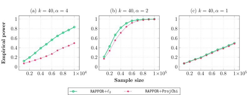
Figure 5: Comparison of the testing power between RAPPOR+$\ell_{2}$ and RAPPOR+ProjChi under the power law alternatives in (99). To ensure a fair comparison, both tests are calibrated using permutation procedures at level $\gamma=0.05$.

The results presented in Figure 5 demonstrate that in this power law scenario, where the signal is strong in $\ell_{2}$ distance and weak in chi-square divergence, RAPPOR+$\ell_{2}$ outperforms RAPPOR+ProjChi. This difference is more pronounced in the low-privacy setting (meaning larger $\alpha$ values) and becomes more subtle as the privacy level increases (meaning smaller $\alpha$ values).

An intuition behind this phenomenon is as follows. For each $m\in[k]$, the $m$th entry of the RAPPOR output follows $\mathrm{Ber}\left(\alpha_{\mathrm{bf}}\mathds{1}(Y_{i}=m)+\delta_{\mathrm{bf}}\right),$ where $\alpha_{\mathrm{bf}}=\alpha/4+o(\alpha)$ and $\delta_{\mathrm{bf}}=1/2+o(1)$, with $o(1)$ representing a term that vanishes as $\alpha\to 0$. Threrfore, as $\alpha$ decreases, the distributions approach uniform multinomial distributions, diminishing the difference between chi-square divergence and $\ell_{2}$ distance in the signal.

G.3 Numerical Result for Density Testing for Scale Alternatives

Similar to the location alternative scenario (19), we analyze scenarios involving covariance differences between two $d$-dimensional Gaussian distributions $P_{\mathbf{Y}}=\mathcal{N}(\bm{\mu}_{\mathbf{Y}},\Sigma_{\mathbf{Y}})$ and $P_{\mathbf{Z}}=\mathcal{N}(\bm{\mu}_{\mathbf{Z}},\Sigma_{\mathbf{Z}})$. We set the mean vectors and covariance matrices of the Gaussian distributions as

$$\bm{\mu}_{\mathbf{Y}}=\bm{\mu}_{\mathbf{Z}}=\mathbf{0}_{d},\Sigma_{\mathbf{Y}}=0.5\times\mathbf{J}_{d}+0.5\times\mathbf{I}_{d},\quad\text{and}\quad\Sigma_{\mathbf{Z}}=5\times\Sigma_{\mathbf{Y}}.$$ (100)

The power results against the scale alternatives, provided in Figure 6, shows similar patterns to Figure 4.

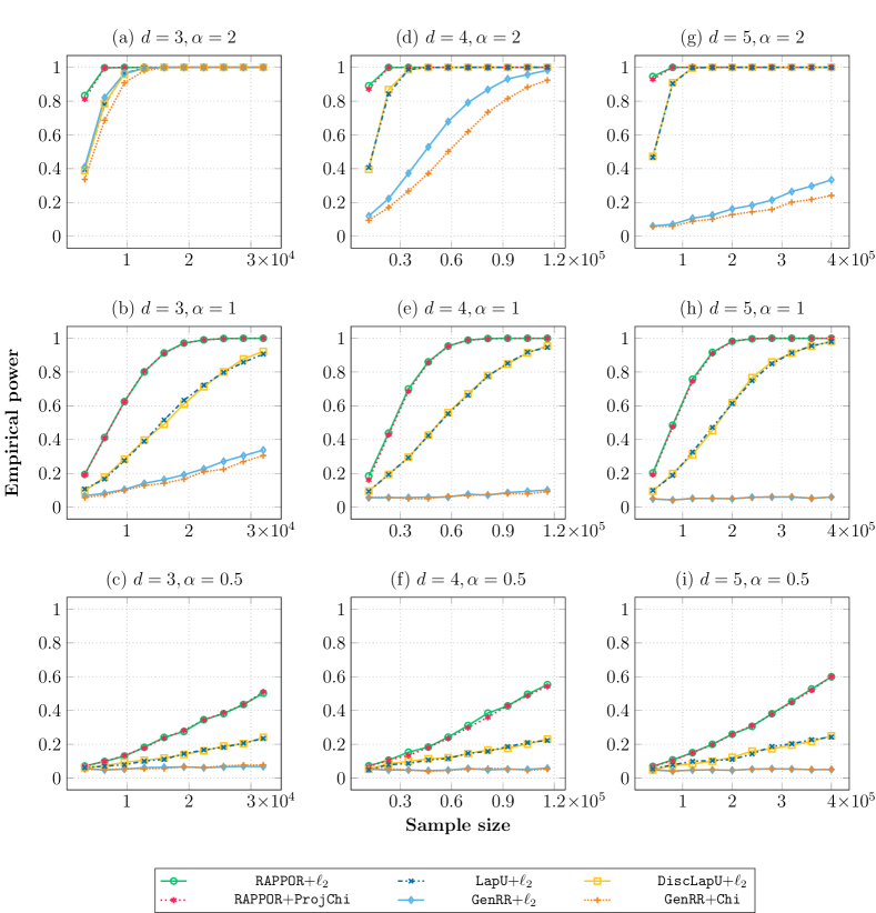
Figure 6: Comparison of the density testing power between our proposed methods (first row in the legend) and baseline methods (second row in the legend) under the scale alternatives in (100). To ensure a fair comparison, all methods are calibrated using permutation procedures at level $\gamma=0.05$.

G.4 Proof of Asymptotic Null Distributions

This section presents the derivation of chi-square asymptotic null distributions of GenRR+Chi and RAPPOR+Chi $\alpha$-LDP tests introduced in Appendix G.1, starting with GenRR+Chi.

G.4.1 Proof of Lemma G.2

The proof is a straighforward application of Lindberg’s CLT.

Proof.

Throughout the proof, assume that the null hypothesis $\mathbf{p}_{Y}=\mathbf{p}_{Z}$ holds. Thus, for each $m\in[k]$, we have $p_{{\tilde{Y}}{m}}=p_{{\tilde{Z}}{m}}$. Without loss of generality, we denote all $p_{{\tilde{Z}}{m}}$ as $p_{{\tilde{Y}}{m}}$. For each $i\in[n_{1}]$ and $j\in[n_{2}]$, we can view $\tilde{Y}_{i}$ and $\tilde{Z}_{j}$ as drawn independently from a multinomial distribution with probability vector defined as:

$$\mathbf{p}_{\tilde{Y}}:=\frac{\exp(\alpha)}{\exp(\alpha)+k-1}\mathbf{p}_{Y}+\frac{1}{\exp(\alpha)+k-1}(\mathbf{1}_{k}-\mathbf{p}_{Y}).$$ (101)

For each $m\in[k]$, the $m$th term of $\hat{\bm{\mu}}_{\tilde{Y}}-\hat{\bm{\mu}}_{\tilde{Y}}$ can be written as

$$\hat{{\mu}}_{\tilde{Y}m}-\hat{{\mu}}_{\tilde{Z}m}=\frac{1}{n_{1}}\sum_{i=1}^{n_{1}}\bigl{(}\mathds{1}(\tilde{Y}_{i}=m)-p_{{\tilde{Y}}{m}}\bigr{)}-\frac{1}{n_{2}}\sum_{j=1}^{n_{2}}\bigl{(}\mathds{1}(\tilde{Z}_{j}=m)-p_{{\tilde{Y}}{m}}\bigr{)}.$$

To apply Lindeberg’s CLT, we construct a triangular array sequence. Each row of the array corresponds to the pooled sample size $N\coloneqq n_{1}+n_{2}$. Within each row, the columns are indexed by $\ell\in[N]$. For each $N$ and $\ell$, we define a $k$-dimensional random vector $\tilde{\mathbf{X}}_{N[:,\ell]}$, whose $m$th element, denoted as $\tilde{\mathbf{X}}_{N[m,\ell]}$, is given by:

$$\tilde{\mathbf{X}}_{N[m,\ell]}:=\begin{cases}\sqrt{\biggl{(}\dfrac{1}{n_{1}}+\dfrac{1}{n_{2}}\biggr{)}^{-1}}\dfrac{1}{n_{1}}\bigl{(}\mathds{1}(\tilde{Y}_{\ell}=m)-p_{{\tilde{Y}}{m}}\bigr{)}\leavevmode\nobreak\ &\text{if}\leavevmode\nobreak\ 1\leq\ell\leq n_{1},\\ \sqrt{\biggl{(}\dfrac{1}{n_{1}}+\dfrac{1}{n_{2}}\biggr{)}^{-1}}\dfrac{1}{n_{2}}\bigl{(}p_{{\tilde{Y}}{m}}-\mathds{1}(\tilde{Z}_{\ell-n_{1}}=m)\bigr{)}\leavevmode\nobreak\ &\text{if}\leavevmode\nobreak\ (n_{1}+1)\leq\ell\leq(n_{1}+n_{2}),\end{cases}$$

for $m\in[k]$. Then for each $\ell\in[N]$, we have $\mathbb{E}[\tilde{\mathbf{X}}_{N[:,\ell]}]=0$ and

$$\sum_{\ell=1}^{N}\tilde{\mathbf{X}}_{N[:,\ell]}=\sqrt{\biggl{(}\dfrac{1}{n_{1}}+\dfrac{1}{n_{2}}\biggr{)}^{-1}}(\hat{\bm{\mu}}_{\tilde{Y}}-\hat{\bm{\mu}}_{\tilde{Z}}).$$

We also have:

$$\mathrm{Cov}(\tilde{\mathbf{X}}_{N[:,\ell]})=\begin{cases}\biggl{(}\dfrac{1}{n_{1}}+\dfrac{1}{n_{2}}\biggr{)}^{-1}\dfrac{1}{n_{1}^{2}}\bigl{(}\text{diag}(\mathbf{p}_{\tilde{Y}})-\mathbf{p}_{\tilde{Y}}\mathbf{p}_{\tilde{Y}}^{\top}\bigr{)}\leavevmode\nobreak\ &\text{if}\leavevmode\nobreak\ 1\leq\ell\leq n_{1},\\ \biggl{(}\dfrac{1}{n_{1}}+\dfrac{1}{n_{2}}\biggr{)}^{-1}\dfrac{1}{n_{2}^{2}}\bigl{(}\text{diag}(\mathbf{p}_{\tilde{Y}})-\mathbf{p}_{\tilde{Y}}\mathbf{p}_{\tilde{Y}}^{\top}\bigr{)}\leavevmode\nobreak\ &\text{if}\leavevmode\nobreak\ (n_{1}+1)\leq\ell\leq(n_{1}+n_{2}).\end{cases}$$

Now we verify two conditions of Lindberg’s CLT in order.

Condition 1: Convergence of the sum of covariances. We aim to verify the following condition:

$$\sum_{\ell=1}^{N}\mathrm{Cov}(\tilde{\mathbf{X}}_{N[:,\ell]})\to\Sigma\leavevmode\nobreak\ \text{as}\leavevmode\nobreak\ N\to\infty,$$ (102)

for some fixed covariance matrix $\Sigma$. The condition (102) is verified as follows. For each $N$,

$$\sum_{\ell=1}^{N}\mathrm{Cov}(\tilde{\mathbf{X}}_{N[:,\ell]}) =\biggl{(}\dfrac{1}{n_{1}}+\dfrac{1}{n_{2}}\biggr{)}^{-1}\left(\sum_{i=1}^{n_{1}}\frac{1}{n_{1}^{2}}\bigl{(}\text{diag}(\mathbf{p}_{\tilde{Y}})-\mathbf{p}_{\tilde{Y}}\mathbf{p}_{\tilde{Y}}^{\top}\bigr{)}+\sum_{j=1}^{n_{2}}\frac{1}{n_{2}^{2}}\bigl{(}\text{diag}(\mathbf{p}_{\tilde{Y}})-\mathbf{p}_{\tilde{Y}}\mathbf{p}_{\tilde{Y}}^{\top}\bigr{)}\right)$$

$$=\text{diag}(\mathbf{p}_{\tilde{Y}})-\mathbf{p}_{\tilde{Y}}\mathbf{p}_{\tilde{Y}}^{\top}.$$

Since the covariance computed above depends on neither $N$ nor $\ell$, the condition (102) holds for $\Sigma=\text{diag}(\mathbf{p}_{\tilde{Y}})-\mathbf{p}_{\tilde{Y}}\mathbf{p}_{\tilde{Y}}^{\top}.$ Now we check the second condition of Lindberg’s CLT:

Condition 2: Lindberg’s condition. We aim to verify the following condition:

$$\sum_{\ell=1}^{N}\mathbb{E}\bigl{[}\|\tilde{\mathbf{X}}_{N[:,\ell]}\|_{2}^{2}\mathds{1}\left(\|\tilde{\mathbf{X}}_{N[:,\ell]}\|_{2}>\epsilon\right)\bigr{]}\to 0\leavevmode\nobreak\ \text{as}\leavevmode\nobreak\ N\to\infty,\leavevmode\nobreak\ \text{for any}\leavevmode\nobreak\ \epsilon>0.$$ (103)

The condition (103) is verified as follows. For any fixed $\ell$, we have:

$$\|\tilde{\mathbf{X}}_{N[:,\ell]}\|_{2}=\begin{cases}\sqrt{\biggl{(}\dfrac{1}{n_{1}}+\dfrac{1}{n_{2}}\biggr{)}^{-1}}\dfrac{1}{n_{1}}\bigl{\{}\sum_{m=1}^{k}\bigl{(}\mathds{1}(\tilde{Y}_{\ell}=m)-p_{{\tilde{Y}}{m}}\bigr{)}^{2}\bigr{\}}^{1/2}\leavevmode\nobreak\ &\text{if}\leavevmode\nobreak\ \ell=1,\ldots,n_{1},\\ \sqrt{\biggl{(}\dfrac{1}{n_{1}}+\dfrac{1}{n_{2}}\biggr{)}^{-1}}\dfrac{1}{n_{2}}\bigl{\{}\sum_{m=1}^{k}\bigl{(}\mathds{1}(\tilde{Z}_{\ell-n_{1}}=m)-p_{{\tilde{Y}}{m}}\bigr{)}^{2}\bigr{\}}^{1/2}\leavevmode\nobreak\ &\text{if}\leavevmode\nobreak\ (n_{1}+1)\leq\ell\leq(n_{1}+n_{2}).\end{cases}$$ (104)

Note that $|\mathds{1}(\tilde{Y}_{\ell}=m)-p_{{\tilde{Y}}{m}}|\leq 1$ and $|\mathds{1}(\tilde{Z}_{\ell-n_{1}}=m)-p_{{\tilde{Y}}{m}}|\leq 1$ for $m\in[k]$. Therefore, for any $\ell\in[N]$, we have the following upper bound:

$$\|\tilde{\mathbf{X}}_{N[:,\ell]}\|_{2}\leq\sqrt{\biggl{(}\dfrac{1}{n_{1}}+\dfrac{1}{n_{2}}\biggr{)}^{-1}}\frac{\sqrt{k}}{\min(n_{1},n_{2})},$$

where the right-hand side is not random and does not depend on $\ell$. Therefore, when verifying the condition (103), we can pull the indicator out of the expectation and the sum:

$$\sum_{\ell=1}^{N}\mathbb{E}\bigl{[}\|\tilde{\mathbf{X}}_{N[:,\ell]}\|_{2}^{2}\mathds{1}\left(\|\tilde{\mathbf{X}}_{N[:,\ell]}\|_{2}>\epsilon\right)\bigr{]} \leq\sum_{\ell=1}^{N}\mathbb{E}\Biggl{[}\|\tilde{\mathbf{X}}_{N[:,\ell]}\|_{2}^{2}\mathds{1}\Biggl{(}\sqrt{\biggl{(}\dfrac{1}{n_{1}}+\dfrac{1}{n_{2}}\biggr{)}^{-1}}\frac{\sqrt{k}}{\min(n_{1},n_{2})}>\epsilon\Biggr{)}\Biggr{]}$$

$$=\mathds{1}\left(\sqrt{\biggl{(}\dfrac{1}{n_{1}}+\dfrac{1}{n_{2}}\biggr{)}^{-1}}\frac{\sqrt{k}}{\min(n_{1},n_{2})}>\epsilon\right)\sum_{\ell=1}^{N}\mathbb{E}\bigl{[}\|\tilde{\mathbf{X}}_{N[:,\ell]}\|_{2}^{2}\bigr{]}.$$

From (104), it can be shown that $\sum_{\ell=1}^{N}\mathbb{E}\bigl{[}\|\tilde{\mathbf{X}}_{N[:,\ell]}\|_{2}^{2}\bigr{]}=2\mathrm{tr}\bigl{(}\text{diag}(\mathbf{p}_{\tilde{Y}})-\mathbf{p}_{\tilde{Y}}\mathbf{p}_{\tilde{Y}}^{\top}\bigr{)},$ where the right-hand side is finite and do not depend on $N$. For any $n_{1}$ and $n_{2}$ large enough, we have

$$\sqrt{\biggl{(}\dfrac{1}{n_{1}}+\dfrac{1}{n_{2}}\biggr{)}^{-1}}\frac{\sqrt{k}}{\min(n_{1},n_{2})}=\sqrt{\frac{n_{1}n_{2}}{n_{1}+n_{2}}}\frac{\sqrt{k}}{\min(n_{1},n_{2})}<\epsilon.$$

Therefore, the condition (103) is satisfied when $n_{1},n_{2}\to\infty$. Therefore by Lindberg’s CLT, we have

$$\sum_{\ell=1}^{N}\tilde{\mathbf{X}}_{N[:,\ell]}=\sqrt{\biggl{(}\dfrac{1}{n_{1}}+\dfrac{1}{n_{2}}\biggr{)}^{-1}}(\hat{\mathbf{\mu}}_{\tilde{Y}}-\hat{\mathbf{\mu}}_{\tilde{Z}})\stackrel{{\scriptstyle d}}{{\to}}\mathcal{N}\bigl{(}0,\text{diag}(\mathbf{p}_{\tilde{Y}}\bigr{)}-\mathbf{p}_{\tilde{Y}}\mathbf{p}_{\tilde{Y}}^{\top}).$$

By the weak law of large numbers and Slutsky’s theorem, it can be shown that

$$\sqrt{\biggl{(}\dfrac{1}{n_{1}}+\dfrac{1}{n_{2}}\biggr{)}^{-1}}\mathrm{diag}(\hat{\mathbf{p}})^{-1/2}(\hat{\mathbf{\mu}}_{\tilde{Y}}-\hat{\mathbf{\mu}}_{\tilde{Z}})\stackrel{{\scriptstyle d}}{{\to}}\mathcal{N}\bigl{(}0,I_{k}-\mathrm{diag}(\mathbf{p}_{\tilde{Y}})^{-1/2}\mathbf{p}_{\tilde{Y}}\mathbf{p}_{\tilde{Y}}^{\top}\mathrm{diag}(\mathbf{p}_{\tilde{Y}})^{-1/2}\bigr{)}.$$ (105)

Since the covariance matrix in (105) is an identity matrix minus a rank-one matrix formed by an orthonormal vector, its eigenvalues are 0 (with multiplicity 1) and 1 (with multiplicity $k-1$). Thus, the covariance matrix is a projection matrix of rank $k-1$. By a standard result (for example, Lemma 17.1 of van der Vaart,, 1998), the test statistic in (96), equivalent to the squared $\ell_{2}$ norm of the left-hand side of (105), converges to a chi-square distribution with $k-1$ degrees of freedom. This concludes the proof of Lemma G.2. ∎

G.4.2 Proof of Lemma G.3

The proof is a straightforward application of Lindberg’s CLT.

Proof.

Throughout the proof, assume that the null hypothesis $\mathbf{p}_{Y}=\mathbf{p}_{Z}$ holds. Thus, for each $m\in[k]$, we have $\mathbb{E}(\tilde{Y}_{1m})=\mathbb{E}(\tilde{Z}_{1m})$. Without loss of generality, we denote all $\mathbb{E}(\tilde{Z}_{1m})$ as $\mathbb{E}(\tilde{Y}_{1m})$. The proof leverages the content and structure of the argument used in the proof for $T_{n_{1},n_{2}}$ in Appendex G.4.1. To apply Lindeberg’s CLT, we construct a triangular array sequence. Each row of the array corresponds to the pooled sample size $N\coloneqq n_{1}+n_{2}$. Within each row, the columns are indexed by $\ell\in[N]$. For each $N$ and $\ell$, we define a $k$-dimensional random vector $\tilde{\mathbf{X}}_{N[:,\ell]}$,whose $m$th element, denoted as $\tilde{\mathbf{X}}_{N[m,\ell]}$, is given by:

$$\tilde{\mathbf{X}}_{N[m,\ell]}:=\begin{cases}\sqrt{\biggl{(}\dfrac{1}{n_{1}}+\dfrac{1}{n_{2}}\biggr{)}^{-1}}\dfrac{1}{n_{1}}\bigl{(}\tilde{Y}_{\ell m}-\mathbb{E}(\tilde{Y}_{1m})\bigr{)}\leavevmode\nobreak\ &\text{if}\leavevmode\nobreak\ 1\leq\ell\leq n_{1},\\ \sqrt{\biggl{(}\dfrac{1}{n_{1}}+\dfrac{1}{n_{2}}\biggr{)}^{-1}}\dfrac{1}{n_{2}}\bigl{(}\mathbb{E}(\tilde{Y}_{1m})-\tilde{Z}_{(\ell-n_{1})m}\bigr{)}\leavevmode\nobreak\ &\text{if}\leavevmode\nobreak\ (n_{1}+1)\leq\ell\leq(n_{1}+n_{2}),\end{cases}$$

for $m\in[k]$, where we recall from (53) that

$$\mathbb{E}(\tilde{Y}_{1m})=\frac{(e^{\alpha/2}-1)p_{{Y}{m}}+1}{e^{\alpha/2}+1}.$$

Now we verify two conditions of Lindberg’s CLT in order.

Condition 1: Convergence of the sum of covariances. To verify the condition (102), first note that:

$$\sum_{\ell=1}^{N}\mathrm{Cov}(\tilde{\mathbf{X}}_{N[:,\ell]}) =\biggl{(}\dfrac{1}{n_{1}}+\dfrac{1}{n_{2}}\biggr{)}^{-1}\left(\sum_{i=1}^{n_{1}}\frac{1}{n_{1}^{2}}\mathrm{Cov}(\tilde{\mathbf{Y}_{i}})+\sum_{j=1}^{n_{2}}\frac{1}{n_{2}^{2}}\mathrm{Cov}(\tilde{\mathbf{Z}_{j}})\right)$$

$$=\mathrm{Cov}(\tilde{\mathbf{Y}}_{1})$$

$$=\left(\frac{e^{\alpha/2}-1}{e^{\alpha/2}+1}\right)^{2}\bigl{(}\mathrm{diag}(\mathbf{p}_{Y})-\mathbf{p}_{Y}{\mathbf{p}^{\top}_{Y}}\bigr{)}+\frac{e^{\alpha/2}}{(e^{\alpha/2}+1)^{2}}I_{d},$$

where the last calculation is from Lemma B.2. Since the covariance computed above depends on neither $N$ nor $\ell$, the condition (102) is satisfied with $\Sigma=\mathrm{Cov}(\tilde{\mathbf{Y}}_{1})$.

Condition 2: Lindberg’s condition. To verify the condition (103) , first note that $0\leq\tilde{Y}_{\ell m}-\mathbb{E}(\tilde{Y}_{1m})\leq 1$ and $0\leq\mathbb{E}(\tilde{Y}_{1m})-\tilde{Z}_{(\ell-n_{1})m}\leq 1$. Therefore by the same analysis as the proof of $T_{n_{1},n_{2}}$, the condition (103) is also satisfied. Therefore, by Linbderg’s CLT, we have:

$$\sqrt{\biggl{(}\dfrac{1}{n_{1}}+\dfrac{1}{n_{2}}\biggr{)}^{-1}}(\check{\mathbf{Y}}-\check{\mathbf{Z}})\stackrel{{\scriptstyle d}}{{\to}}\mathcal{N}(0,\mathrm{Cov}(\tilde{\mathbf{Y}}_{1})).$$ (106)

Note that $\mathrm{Cov}(\tilde{\mathbf{Y}}_{1})$ has an eigenvector $\mathbf{1}$, which corresponds to an eigenvalue which is neither $0$ nor $1$. To turn the covariance matrix into a projection matrix, we delete the eigenvector $\mathbf{1}$ by pre-multiplying the random vector in the left-hand side of (106) by $\mathrm{Cov}(\tilde{\mathbf{Y}}_{1})^{-1/2}\Pi$. Then we have:

$$\mathrm{Cov}(\tilde{\mathbf{Y}_{1}})^{-1/2}\Pi\sqrt{\biggl{(}\dfrac{1}{n_{1}}+\dfrac{1}{n_{2}}\biggr{)}^{-1}}(\check{\mathbf{Y}}-\check{\mathbf{Z}})\stackrel{{\scriptstyle d}}{{\to}}\mathcal{N}\bigl{(}0,\mathrm{Cov}(\tilde{\mathbf{Y}}_{1})^{-1/2}\Pi\mathrm{Cov}(\tilde{\mathbf{Y}}_{1})\Pi\mathrm{Cov}(\tilde{\mathbf{Y}}_{1})^{-1/2}\bigr{)}.$$

For a map $h:A\to A^{-1/2}$, define $\mathrm{Disc}(h):=\{A\in\mathbb{R}^{p\times p}:h\leavevmode\nobreak\ \text{is not continuous at}\leavevmode\nobreak\ A\}$. By Lemma 5.6 of Gaboardi and Rogers, (2018), $\mathrm{Cov}(\tilde{\mathbf{Y}}_{1})$ is invertible for any $\alpha>0$ and any $\mathbf{p}_{Y}\in\mathrm{int}(\Omega)$. Therefore we have $\mathrm{Cov}(\tilde{\mathbf{Y}}_{1}\bigr{)}\notin\mathrm{Disc}(h)$ almost surely. Thus by the weak law of large numbers and the continuous mapping theorem, we have $\hat{\Sigma}^{-1/2}\stackrel{{\scriptstyle p}}{{\to}}\mathrm{Cov}(\tilde{\mathbf{Y}}_{1})^{-1/2}$. Then by Slutsky’s theorem, we have

$$\hat{\Sigma}^{-1/2}\Pi\sqrt{\biggl{(}\dfrac{1}{n_{1}}+\dfrac{1}{n_{2}}\biggr{)}^{-1}}(\check{\mathbf{Y}}-\check{\mathbf{Z}})\stackrel{{\scriptstyle d}}{{\to}}\mathcal{N}(0,\mathrm{Cov}(\tilde{\mathbf{Y}}_{1})^{-1/2}\Pi\mathrm{Cov}(\tilde{\mathbf{Y}}_{1})\Pi\mathrm{Cov}(\tilde{\mathbf{Y}}_{1})^{-1/2}).$$ (107)

By the analysis of Gaboardi and Rogers, (2018), $\mathrm{Cov}(\tilde{\mathbf{Y}}_{1})^{-1/2}\Pi\mathrm{Cov}(\tilde{\mathbf{Y}_{1}})\Pi\mathrm{Cov}(\tilde{\mathbf{Y}}_{1})^{-1/2}$ is an identity matrix except one of the entries on the diagonal being zero, thus a projection matrix with rank $k-1$. Therefore, by a standard result (for example, Lemma 17.1 van der Vaart,, 1998), the test statistic (97), which is equivalent to squared $\ell_{2}$ norm of the random vector on the left-hand side of (107), converges to a chi-square distribution with $k-1$ degrees of freedom. This concludes the proof of Lemma G.3. ∎

Appendix H Suboptimality of Generalized Randomized Response

This section illustrates that the generalized randomized response mechanism in (95) can lead to suboptimal power. Specifically, we show that the GenRR+$\ell_{2}$ test performs suboptimally in certain privacy regimes where the number of categories $k$ increases with the sample size $n_{1}$, but the privacy level $\alpha$ is fixed. This negative result is further supported by our numerical studies in Section 5.

Theorem H.1 (Asymptotic powerlessness of GenRR+$\ell_{2}$ test).

Let $(\mathbf{p}_{Y},\mathbf{p}_{Z})$ be a pair of data-generating multinomial distributions with $k$ categories, where $\mathbf{p}_{Z}$ is a uniform distribution and $\mathbf{p}_{Y}$ is a perturbed uniform distribution parametrized by $\epsilon>0$. Formally, for each $m\in[k]$, the $m$th entry of $\mathbf{p}_{Y}$ and $\mathbf{p}_{Z}$ are defined as:

$$p_{{Y}{m}}:=\frac{1}{k}+\frac{(-1)^{m}\epsilon}{\sqrt{k}},\quad p_{{Z}{m}}:=\frac{1}{k},$$ (108)

ensuring that $\|\mathbf{p}_{Y}-\mathbf{p}_{Z}\|_{2}=\epsilon$. Assume the privacy parameter $\alpha>0$ is sufficiently small so that the minimax testing rate, given in equation (6), satisfies

$$\rho^{\ast}_{n_{1},n_{2},\alpha}\asymp\frac{k^{1/4}}{(n_{1}\alpha^{2})^{1/2}}.$$ (109)

For a sufficiently large, but fixed constant $C>0$, set

$$\epsilon=\frac{C\cdot k^{1/4}}{(n_{1}\alpha^{2})^{1/2}},$$ (110)

and consider the regime where

$$\sqrt{k}\epsilon=\frac{C\cdot k^{3/4}}{(n_{1}\alpha^{2})^{1/2}}\to 0,$$ (111)

which guarantees that $0<p_{{Y}{m}}<1$ in (108) for each $m\in[k]$ and for sufficiently large $n_{1}$. Under this regime, the GenRR+$\ell_{2}$ test is asymptotically powerless, meaning its asymptotic power becomes at most the size.

Given the setting in (110) from Theorem H.1, an optimal test would achieve non-trivial power greater than the significance level by selecting a sufficiently large $C$. However, Theorem H.1 proves that the GenRR+$\ell_{2}$ test becomes asymptotically powerless for any fixed $C>0$, thereby underscoring its suboptimality.

Proof.

For the proof, we analyze the power function of the test statistic. To achieve this, we use high-dimensional asymptotics for U-statistics, specifically Corollary 3.3 and Theorem 3.3 from Kim, (2020), which are restated as Theorem B.1 and Theorem B.2, respectively.

Let $w:=(e^{\alpha}-1)/(e^{\alpha}+k-1)$. Recall from (101) that the $\alpha$-LDP view $\{\tilde{Y}_{i}\}_{i\in[n_{1}]}$ via GenRR mechanism is equivalent to a random sample drawn from a mixture of $\mathbf{p}_{Y}$ and $\mathbf{p}_{Z}$ defined as follows:

$$\mathbf{p}_{\tilde{Y}} :=\frac{e^{\alpha}}{e^{\alpha}+k-1}\mathbf{p}_{Y}+\frac{1}{e^{\alpha}+k-1}(\mathbf{1}_{k}-\mathbf{p}_{Y})$$

$$=\frac{e^{\alpha}-1}{e^{\alpha}+k-1}\mathbf{p}_{Y}+\frac{k}{e^{\alpha}+k-1}\frac{1}{k}\mathbf{1}_{k}$$

$$=w\mathbf{p}_{Y}+(1-w)\mathbf{p}_{Z},$$ (112)

Similarly, $\{\tilde{Z}_{i}\}_{i\in[n_{2}]}$ can be viewed as a random sample drawn from $\mathbf{p}_{\tilde{Z}}:=w\mathbf{p}_{Z}+(1-w)\mathbf{p}_{Z}=\mathbf{p}_{Z}$. Note that the $\ell_{2}$ distance between the probability vectors shrinks to $\|\mathbf{p}_{\tilde{Y}}-\mathbf{p}_{\tilde{Z}}\|_{2}=w\epsilon$.

For convenience, let $\{\tilde{\mathbf{Y}}_{i}\}_{i\in[n_{1}]}$ be the one-hot vectorized version of $\{\tilde{Y}_{i}\}_{i\in[n_{1}]}$. We define a one-sample U-statistic for uniformity testing as follows:

$$U_{n_{1}}:=\frac{2}{n_{1}(n_{1}-1)}\sum_{1\leq i<j\leq n_{1}}h(\tilde{\mathbf{Y}}_{i},\tilde{\mathbf{Y}}_{j}),$$ (113)

where $h(\tilde{\mathbf{Y}}_{i},\tilde{\mathbf{Y}}_{j}):=\bigl{(}\tilde{\mathbf{Y}}_{i}-\mathbf{p}_{Z}\bigr{)}^{\top}\bigl{(}\tilde{\mathbf{Y}}_{j}-\mathbf{p}_{Z}\bigr{)}$, which is a special case of the two-sample statistic $U_{n_{1},n_{2}}$ in (9) with $n_{2}=\infty$. Now we analyze the power function of the test based on $U_{n_{1}}$ by specifying the critical value, the distribution of the test statistic under the alternative, and the power function in order.

Critical value. We specify the critical value by establishing the asymptotic normality of the test statistic under the null by utilizing Theorem B.1. Since the statistic (113) is equivalent to the statistic $U_{I}$ in (31) of Theorem B.1, it suffices to show that $n_{1}/\sqrt{k}\to\infty$ to establish the asymptotic normality. Note that the assumption $\sqrt{k}\epsilon=Ck^{3/4}/(n_{1}\alpha^{2})^{1/2}\to 0$ in (111) implies $n_{1}/\sqrt{k}\to\infty$ for fixed $\alpha$. Therefore, under the null of $\mathbf{p}_{Y}=\mathbf{p}_{Z}$, which implies $\mathbf{p}_{\tilde{Y}}=w\mathbf{p}_{Z}+(1-w)\mathbf{p}_{Z}=\mathbf{p}_{Z}$, we have

$$\sqrt{\binom{n_{1}}{2}}\frac{U_{n_{1}}}{\sqrt{k^{-1}(1-k^{-1})}}\overset{d}{\longrightarrow}\mathcal{N}(0,1).$$

Based on this asymptotic normality, an asymptotically exact critical value is specified as follows:

$$\text{Reject}\leavevmode\nobreak\ H_{0}\leavevmode\nobreak\ \text{if}\leavevmode\nobreak\ U_{n_{1}}\geq z_{\gamma}\sqrt{\frac{2(1-1/k)}{kn_{1}(n_{1}-1)}}.$$ (114)

Here $z_{\gamma}$ denotes the upper $\gamma$ quantile of $W\sim\mathcal{N}(0,1)$ satisfying $\mathbb{P}(W>z_{\gamma})=\gamma$.

Alternative distribution. Next we derive that the asymptotic distribution of the test statistic under the alternative specified in (108). By substituting $\|\mathbf{p}_{\tilde{Y}}-\mathbf{p}_{Z}\|_{2}^{2}=w^{2}\epsilon^{2}$ into (32), we can establish the following asymptotic normality:

$$\sqrt{\frac{n_{1}(n_{1}-1)}{2}}\frac{U_{n_{1}}-w^{2}\epsilon^{2}}{\sqrt{\mathrm{tr}(\Sigma_{\tilde{Y}}^{2})+2(n_{1}-1)(\mathbf{p}_{\tilde{Y}}-\mathbf{p}_{Z})^{\top}\Sigma_{\tilde{Y}}(\mathbf{p}_{\tilde{Y}}-\mathbf{p}_{Z})}}\stackrel{{\scriptstyle d}}{{\to}}\mathcal{N}(0,1),$$ (115)

provided that the conditions C1, C2, and C3 of Theorem B.2 hold. We verify these conditions in order.

Verification of the condition C1. The condition C1 is restated as follows:

$$\frac{\mathrm{tr}(\Sigma_{\tilde{Y}}^{4})}{\bigl{\{}\mathrm{tr}(\Sigma_{\tilde{Y}}^{2})\bigr{\}}^{2}}\to 0.$$

We first analyze the denominator $\bigl{\{}\mathrm{tr}(\Sigma_{\tilde{Y}}^{2})\bigr{\}}^{2}$. Since $\Sigma_{\tilde{Y}}=\mathrm{diag}(\mathbf{p}_{\tilde{Y}})-\mathbf{p}_{\tilde{Y}}\mathbf{p}_{\tilde{Y}}^{\top}$, we have

$$\Sigma_{\tilde{Y}}^{2}=\{\mathrm{diag}(\mathbf{p}_{\tilde{Y}})\}^{2}+(\mathbf{p}_{\tilde{Y}}\mathbf{p}_{\tilde{Y}}^{\top})^{2}-\mathrm{diag}(\mathbf{p}_{\tilde{Y}})\mathbf{p}_{\tilde{Y}}\mathbf{p}_{\tilde{Y}}^{\top}-\mathbf{p}_{\tilde{Y}}\mathbf{p}_{\tilde{Y}}^{\top}\mathrm{diag}(\mathbf{p}_{\tilde{Y}}).$$

Utilizing the equalities $\bigl{(}\mathbf{p}_{\tilde{Y}}\mathbf{p}_{\tilde{Y}}^{\top}\bigr{)}^{2}=\|\mathbf{p}_{\tilde{Y}}\|_{2}^{2}\mathbf{p}_{\tilde{Y}}\mathbf{p}_{\tilde{Y}}^{\top}$, $\mathrm{tr}\bigl{(}\mathbf{p}_{\tilde{Y}}\mathbf{p}_{\tilde{Y}}^{\top}\bigr{)}=\|\mathbf{p}_{\tilde{Y}}\|_{2}^{2}$, and $\mathrm{tr}\bigl{(}\text{diag}(\mathbf{p}_{\tilde{Y}})\mathbf{p}_{\tilde{Y}}\mathbf{p}_{\tilde{Y}}^{\top}\bigr{)}=\mathbf{p}_{\tilde{Y}}^{\top}\text{diag}(\mathbf{p}_{\tilde{Y}})\mathbf{p}_{\tilde{Y}}$, we can calculate $\mathrm{tr}(\Sigma_{\tilde{Y}}^{2})$ as

$$\mathrm{tr}(\Sigma_{\tilde{Y}}^{2})=\|\mathbf{p}_{\tilde{Y}}\|_{2}^{2}+\|\mathbf{p}_{\tilde{Y}}\|_{2}^{4}-2\|\mathbf{p}_{\tilde{Y}}\|_{3}^{3}.$$

In a similar manner, we can expand the numerator term as follows:

$$\mathrm{tr}(\Sigma_{\tilde{Y}}^{4})=\|\mathbf{p}_{\tilde{Y}}\|_{4}^{4}+\|\mathbf{p}_{\tilde{Y}}\|_{2}^{8}+2\|\mathbf{p}_{\tilde{Y}}\|_{3}^{6}+4\|\mathbf{p}_{\tilde{Y}}\|_{2}^{2}\|\mathbf{p}_{\tilde{Y}}\|_{4}^{4}-4\|\mathbf{p}_{\tilde{Y}}\|_{2}^{4}\|\mathbf{p}_{\tilde{Y}}\|_{3}^{3}-4\|\mathbf{p}_{\tilde{Y}}\|_{5}^{5}.$$

Therefore, it suffices to study the asymptotic behavior of

$$\mathrm{tr} (\Sigma_{\tilde{Y}}^{4})/\bigl{\{}\mathrm{tr}(\Sigma_{\tilde{Y}}^{2})\bigr{\}}^{2}$$

$$=\frac{\bigl{(}\|\mathbf{p}_{\tilde{{Y}}}\|_{2}^{8}-4\|\mathbf{p}_{\tilde{{Y}}}\|_{2}^{4}\|\mathbf{p}_{\tilde{{Y}}}\|_{3}^{3}+2\|\mathbf{p}_{\tilde{{Y}}}\|_{3}^{6}\bigr{)}+\|\mathbf{p}_{\tilde{{Y}}}\|_{4}^{4}+4\|\mathbf{p}_{\tilde{{Y}}}\|_{2}^{2}\|\mathbf{p}_{\tilde{{Y}}}\|_{4}^{4}-4\|\mathbf{p}_{\tilde{{Y}}}\|_{5}^{5}}{\bigl{(}\|\mathbf{p}_{\tilde{Y}}\|_{2}^{8}-4\|\mathbf{p}_{\tilde{Y}}\|_{2}^{4}\|\mathbf{p}_{\tilde{Y}}\|_{3}^{3}+4\|\mathbf{p}_{\tilde{Y}}\|_{3}^{6}\bigr{)}+\|\mathbf{p}_{\tilde{Y}}\|_{2}^{4}+2\|\mathbf{p}_{\tilde{Y}}\|_{2}^{2}\|\mathbf{p}_{\tilde{Y}}\|_{2}^{4}-4\|\mathbf{p}_{\tilde{Y}}\|_{2}^{2}\|\mathbf{p}_{\tilde{Y}}\|_{3}^{3}},$$ (116)

where the parentheses group together terms of the same order. Since $p_{{Y}{m}}=1/k+(-1)^{m}\epsilon/\sqrt{k}$, we have

$$p_{{\tilde{Y}}{m}}=\frac{w}{k}+\frac{w(-1)^{m}\sqrt{k}\epsilon}{k}+\frac{1}{k}-\frac{w}{k}=\frac{1}{k}+\frac{(-1)^{m}w\epsilon}{\sqrt{k}},$$ (117)

for $m\in[k]$. Utilizing (117) and the fact that $k$ is an even integer, the powers of norms of $\mathbf{p}_{\tilde{Y}}$ are calculated as follows:

$$\|\mathbf{p}_{\tilde{Y}}\|_{2}^{2}=\frac{1}{k}+w^{2}\epsilon^{2},\ \|\mathbf{p}_{\tilde{Y}}\|_{3}^{3}=\frac{1}{k^{2}}+\frac{3w^{2}\epsilon^{2}}{k},$$ (118)

$$\|\mathbf{p}_{\tilde{Y}}\|_{4}^{4}=\frac{1}{k^{3}}+6\frac{w^{2}\epsilon^{2}}{k^{2}}+\frac{w^{4}\epsilon^{4}}{k},\ \|\mathbf{p}_{\tilde{Y}}\|_{5}^{5}=\frac{1}{k^{4}}+10\frac{w^{2}\epsilon^{2}}{k^{3}}+5\frac{w^{4}\epsilon^{4}}{k^{2}}.$$

By substituting (118) into (116), and recalling that $w\epsilon$ is of order $k^{-3/4}n_{1}^{-1/2}$, we find that among the terms in (116), the term that converges to 0 the most slowly is $-4/k^{3}$, which comes from $-4\|\mathbf{p}_{\tilde{Y}}\|_{2}^{2}\|\mathbf{p}_{\tilde{Y}}\|_{3}^{3}$ in the denominator. Consequently, the quantity in (118) converges to 0, confirming condition C1 of Theorem B.2.

Verification of the condition C2. The condition C2 is recalled below as

$$\dfrac{\mathbb{E}[W_{1}]+n_{1}\mathbb{E}[W_{2}]}{n_{1}^{2}\big{\{}\mathrm{tr}(\Sigma_{\tilde{Y}}^{2})\big{\}}^{2}}\to 0,$$ (119)

where

$$W_{1} :=\bigl{\{}(\tilde{\mathbf{Y}}_{1}-\mathbf{p}_{Z})^{\top}(\tilde{\mathbf{Y}}_{2}-\mathbf{p}_{Z})\bigr{\}}^{4},$$

$$W_{2} :=\bigl{\{}(\tilde{\mathbf{Y}}_{1}-\mathbf{p}_{Z})^{\top}(\tilde{\mathbf{Y}}_{2}-\mathbf{p}_{Z})\bigr{\}}^{2}\bigl{\{}(\tilde{\mathbf{Y}}_{1}-\mathbf{p}_{Z})^{\top}(\tilde{\mathbf{Y}}_{3}-\mathbf{p}_{Z})\bigr{\}}^{2}.$$

We separately analyze the terms in (119). First for $\mathbb{E}[W_{1}]$, the random variable $W_{1}$ takes two distinct values:

$$W_{1}=\begin{cases}\biggl{(}1-\dfrac{1}{k}\biggr{)}^{4},&\tilde{\mathbf{Y}}_{1}=\tilde{\mathbf{Y}}_{2},\\[10.00002pt] \leavevmode\nobreak\ \dfrac{1}{k^{4}},&\text{otherwise.}\end{cases}$$

Observe that, according to (117), we have

$$\mathbb{P}(\tilde{\mathbf{Y}}_{1}=\tilde{\mathbf{Y}}_{2})=\sum_{m=1}^{k}p_{{\tilde{Y}}{m}}^{2}=\sum_{m=1}^{k}\biggl{(}\frac{1}{k}+\frac{(-1)^{m}w\epsilon}{\sqrt{k}}\biggr{)}^{2}=\frac{1}{k}+w^{2}\epsilon^{2}.$$ (120)

Using the established probability (120), we calculate the target expected value as

$$\mathbb{E}[W_{1}]=-\frac{1}{k^{5}}+\frac{k}{k^{5}}-\frac{k\epsilon^{2}w^{2}}{k^{5}}+\frac{(-1+k)^{4}}{k^{5}}+\frac{(-1+k)^{4}(1+k\epsilon^{2}w^{2})}{k^{5}}.$$

Among the terms in the expectation computed above, the term that converges to 0 most slowly is of order $1/k$, which arises from the fourth term of the numerator. Similarly, for $\mathbb{E}[W_{2}],$ the random variable $W_{2}$ takes on the values as:

$$W_{2}=\begin{cases}\biggl{(}1-\dfrac{1}{k}\biggr{)}^{4},&\tilde{\mathbf{Y}}_{1}=\tilde{\mathbf{Y}}_{2}=\tilde{\mathbf{Y}}_{3},\\[10.00002pt] \leavevmode\nobreak\ \dfrac{1}{k^{2}}\biggl{(}1-\dfrac{1}{k}\biggr{)}^{2},&[\tilde{\mathbf{Y}}_{1}=\tilde{\mathbf{Y}}_{2},\tilde{\mathbf{Y}}_{1}\neq\tilde{\mathbf{Y}}_{3}]\cup[\tilde{\mathbf{Y}}_{1}=\tilde{\mathbf{Y}}_{3},\tilde{\mathbf{Y}}_{1}\neq\tilde{\mathbf{Y}}_{2}]\\[10.00002pt] \dfrac{1}{k^{4}},&\text{otherwise.}\end{cases}$$ (121)

The corresponding probabilities are calculated as

$$\mathbb{P}(\tilde{\mathbf{Y}}_{1}=\tilde{\mathbf{Y}}_{2}=\tilde{\mathbf{Y}}_{3})=\sum_{m=1}^{k}p_{{\tilde{Y}}{m}}^{3}=\|\mathbf{p}_{\tilde{Y}}\|_{3}^{3}\stackrel{{\scriptstyle(a)}}{{=}}\frac{1}{k^{2}}+\frac{3w^{2}\epsilon^{2}}{k},\leavevmode\nobreak\ \text{and}$$

$$\mathbb{P}([\tilde{\mathbf{Y}}_{1}=\tilde{\mathbf{Y}}_{2},\tilde{\mathbf{Y}}_{1}\neq\tilde{\mathbf{Y}}_{3}]\cup[\tilde{\mathbf{Y}}_{1}=\tilde{\mathbf{Y}}_{3},\tilde{\mathbf{Y}}_{1}\neq\tilde{\mathbf{Y}}_{2}])\stackrel{{\scriptstyle(b)}}{{=}}2\mathbb{P}([\tilde{\mathbf{Y}}_{1}=\tilde{\mathbf{Y}}_{2},\tilde{\mathbf{Y}}_{1}\neq\tilde{\mathbf{Y}}_{3}])$$

$$\hskip 206.00037pt=2\sum_{m=1}^{k}p_{{\tilde{Y}}{m}}^{2}(1-p_{{\tilde{Y}}{m}})$$

$$\hskip 206.00037pt=2\|\mathbf{p}_{\tilde{Y}}\|_{2}^{2}-2\|\mathbf{p}_{\tilde{Y}}\|_{3}^{3}$$

$$\hskip 203.50037pt\stackrel{{\scriptstyle(c)}}{{=}}\frac{2}{k}+2w^{2}\epsilon^{2}-\frac{2}{k^{2}}-\frac{6w^{2}\epsilon^{2}}{k},$$

where steps $(a)$ and $(c)$ use the equations in (118) and step $(b)$ uses the independence between samples, as well as the exclusiveness and symmetry of the events. Now $\mathbb{E}[W_{2}]$ is calculated as

$$\mathbb{E}[W_{2}] =\biggl{(}1-\frac{1}{k}\biggr{)}^{4}\biggl{(}\frac{1}{k^{2}}+\frac{3w^{2}\epsilon^{2}}{k}\biggr{)}+\biggl{\{}\frac{1}{k^{2}}\biggl{(}1-\frac{1}{k}\biggr{)}^{2}\biggr{\}}\biggl{(}\frac{2}{k}+2w^{2}\epsilon^{2}-\frac{2}{k^{2}}-\frac{6w^{2}\epsilon^{2}}{k}\biggr{)}$$

$$\quad+\frac{1}{k^{4}}\biggl{(}1-\frac{1}{k^{2}}-\frac{3w^{2}\epsilon^{2}}{k}-\frac{2}{k}-2w^{2}\epsilon^{2}+\frac{2}{k^{2}}+\frac{6w^{2}\epsilon^{2}}{k}\biggr{)},$$ (122)

where the term that converges to $0$ the slowest is of order $1/k^{2}$, originating from the first term on the right-hand side of (122). Finally, the trace term in the denominator is calculated as

$$\mathrm{tr}(\Sigma_{\tilde{Y}}^{2}) =\|\mathbf{p}_{\tilde{Y}}\|_{2}^{2}+\|\mathbf{p}_{\tilde{Y}}\|_{2}^{4}-2\|\mathbf{p}_{\tilde{Y}}\|_{3}^{3}$$

$$=\frac{1}{k}+w^{2}\epsilon^{2}+\frac{1}{k^{2}}+w^{4}\epsilon^{4}+\frac{2w^{2}\epsilon^{2}}{k}-\frac{2}{k^{2}}-\frac{6w^{2}\epsilon^{2}}{k}$$

$$=\frac{1}{k}-\frac{1}{k^{2}}+w^{2}\epsilon^{2}+w^{4}\epsilon^{4}-\frac{4w^{2}\epsilon^{2}}{k},$$ (123)

where the term that converges to 0 the slowest is $1/k$. Now to verify the condition C2, we separately analyze the asymptotic behaviors of $\mathbb{E}[W_{1}]/n_{1}^{2}\big{\{}\mathrm{tr}(\Sigma_{\tilde{Y}}^{2})\big{\}}^{2}$ and $n_{1}\mathbb{E}[W_{2}]/n_{1}^{2}\big{\{}\mathrm{tr}(\Sigma_{\tilde{Y}}^{2})\big{\}}^{2}$, focusing on the terms that converges the slowest to $0$ in the numerator and denominator, respectively. For the first term, it suffices to investigate $(1/k)/(n_{1}^{2}/k^{2})$, which converges to 0 as long as $k/n_{1}^{2}\to 0$. Note that $k/n_{1}^{2}\to 0$ is implied by our assumption (111). For the second term, it suffices to investigate $(n_{1}/k^{2})/(n_{1}^{2}/k^{2})$, which converges to 0. Therefore the convergence in (119) is verified, confirming the condition C2 of Theorem B.2.

Verification of the condition C3. The condition C3 is restated as

$$(\mathbf{p}_{\tilde{Y}}-\mathbf{p}_{Z})^{\top}\Sigma_{\tilde{{Y}}}(\mathbf{p}_{\tilde{Y}}-\mathbf{p}_{Z})=o\left(n_{1}^{-1}\mathrm{tr}(\Sigma_{\tilde{{Y}}}^{2})\right).$$ (124)

To calculate the quadratic form therein, note that since $\mathbf{p}_{\tilde{Y}}-\mathbf{p}_{Z}=w(\mathbf{p}_{Y}-\mathbf{p}_{Z})$, we have

$$(\mathbf{p}_{\tilde{Y}}-\mathbf{p}_{Z})^{\top}\Sigma_{\tilde{{Y}}}(\mathbf{p}_{\tilde{Y}}-\mathbf{p}_{Z})=w^{2}(\mathbf{p}_{Y}-\mathbf{p}_{Z})^{\top}\mathrm{diag}(\mathbf{p}_{\tilde{Y}})(\mathbf{p}_{Y}-\mathbf{p}_{Z})-w^{2}(\mathbf{p}_{Y}-\mathbf{p}_{Z})^{\top}\mathbf{p}_{\tilde{Y}}\mathbf{p}_{\tilde{Y}}^{\top}(\mathbf{p}_{Y}-\mathbf{p}_{Z}).$$

We separately analyze the two terms on the right-hand side. For the first term, we have

$$w^{2}(\mathbf{p}_{Y}-\mathbf{p}_{Z})^{\top}\mathrm{diag}(\mathbf{p}_{\tilde{Y}})(\mathbf{p}_{Y}-\mathbf{p}_{Z}) =w^{2}\sum_{m=1}^{k}\frac{(-1)^{m}\epsilon}{\sqrt{k}}\biggl{(}\frac{1}{k}+\frac{(-1)^{m}w\epsilon}{\sqrt{k}}\biggr{)}\frac{(-1)^{m}\epsilon}{\sqrt{k}}$$

$$=\frac{w^{2}\epsilon^{2}}{k}\sum_{m=1}^{k}\biggl{(}\frac{1}{k}+\frac{(-1)^{m}w\epsilon}{\sqrt{k}}\biggr{)}$$

$$=\frac{w^{2}\epsilon^{2}}{k},$$

where the last equality holds since $k$ is even. The second term is computed as

$$w^{2}(\mathbf{p}_{Y}-\mathbf{p}_{Z})^{\top}\mathbf{p}_{\tilde{Y}}\mathbf{p}_{\tilde{Y}}^{\top}(\mathbf{p}_{Y}-\mathbf{p}_{Z}) =w^{2}\bigl{\{}(\mathbf{p}_{Y}-\mathbf{p}_{Z})^{\top}\mathbf{p}_{\tilde{Y}}\bigr{\}}^{2}$$

$$=w^{2}\biggl{\{}\sum_{m=1}^{k}\frac{(-1)^{m}\epsilon}{\sqrt{k}}\biggl{(}\frac{1}{k}+\frac{(-1)^{m}w\epsilon}{\sqrt{k}}\biggr{)}\biggr{\}}^{2}$$

$$=w^{4}\epsilon^{4},$$

where the last equality again uses the fact that $k$ is an even integer. Therefore we have

$$(\mathbf{p}_{\tilde{Y}}-\mathbf{p}_{Z})^{\top}\Sigma_{\tilde{{Y}}}(\mathbf{p}_{\tilde{Y}}-\mathbf{p}_{Z})=\frac{w^{2}\epsilon^{2}}{k}-w^{4}\epsilon^{4},$$ (125)

where $w^{2}\epsilon^{2}/k$ is the term that converges to 0 most slowly. Utilizing the trace calculation (123), we can verify the condition C3 (124) by studying the asymptotic behavior of $(w^{2}\epsilon^{2}/k)/(1/kn_{1})$. Since this quantity converges to 0, the condition C3 is verified.

As all conditions of Theorem B.2 are satisfied, the asymptotic distribution in (115) is confirmed.

Power function. Using the critical value in (114) and the asymptotic alternative distribution established in (115), under the asymptotic regime in (111), the power function is written as:

$$\gamma {}_{n_{1},k,\alpha}(\mathbf{p}_{Y},\mathbf{p}_{Z})$$

$$=\mathbb{P}_{H_{1}}\!\left(U_{n_{1}}\geq z_{\gamma}\sqrt{\frac{2(1-1/k)}{kn_{1}(n_{1}-1)}}\right)$$

$$=\mathbb{P}_{H_{1}}\!\left(W\geq\sqrt{\frac{n_{1}(n_{1}-1)}{2}}\frac{z_{\gamma}\sqrt{2\{1-(1/k)\}/\{kn_{1}(n_{1}-1)\}}-w^{2}\epsilon^{2}}{\sqrt{\mathrm{tr}(\Sigma_{\tilde{Y}}^{2})+2(n_{1}-1)(\mathbf{p}_{\tilde{Y}}-\mathbf{p}_{Z})^{\top}\Sigma_{\tilde{Y}}(\mathbf{p}_{\tilde{Y}}-\mathbf{p}_{Z})}}\right)+o(1)$$

$$=\Phi\!\left(\sqrt{\frac{n_{1}(n_{1}-1)}{2}}\frac{w^{2}\epsilon^{2}-z_{\gamma}\sqrt{2\{1-(1/k)\}/\{kn_{1}(n_{1}-1)\}}}{\sqrt{\mathrm{tr}(\Sigma_{\tilde{Y}}^{2})+2(n_{1}-1)(\mathbf{p}_{\tilde{Y}}-\mathbf{p}_{Z})^{\top}\Sigma_{\tilde{Y}}(\mathbf{p}_{\tilde{Y}}-\mathbf{p}_{Z})}}\right)$$

$$=\Phi\!\left(\frac{\sqrt{n_{1}(n_{1}-1)/2}w^{2}\epsilon^{2}-z_{\gamma}\sqrt{(1/k)-(1/k^{2})}}{\sqrt{\left\{(1/k)-(1/k^{2})+w^{2}\epsilon^{2}+w^{4}\epsilon^{4}-(4w^{2}\epsilon^{2}/k)\right\}+2(n_{1}-1)\bigl{\{}(w^{2}\epsilon^{2}/k)-w^{4}\epsilon^{4}\bigr{\}}}}\right)$$

$$\to\Phi\!\left(-z_{\gamma}\right)=\gamma,$$ (126)

where $W\sim\mathcal{N}(0,1)$, $\Phi$ denotes the cumulative distribution function of $W$, and $o(1)$ refers to a quantity that goes to 0 as $n_{1}$ and $k$ go to $\infty$, in the regime of (111). The last line in (126) uses the fact that given that $w\epsilon$ is of the order $k^{-3/4}n_{1}^{-1/2}$, the term in (126) that converges most slowly to 0 is $\sqrt{1/k}$, which appears both on the second term in the numerator and the first term in the denominator. It is important to note that the convergence result (111) holds for any sufficiently small $\alpha$, indicating that the GenRR+$\ell_{2}$ test becomes asymptotically powerless in the regime where the minimax testing rate is $k^{1/4}/(n_{1}\alpha^{2})^{1/2}$. This completes the proof of Theorem H.1. ∎

References

• (1) Acharya, J., Canonne, C. L., Freitag, C., Sun, Z., and Tyagi, H. (2021a). Inference under information constraints III: Local privacy constraints. IEEE Journal on Selected Areas in Information Theory, 2:253–267.
• Acharya et al., (2019) Acharya, J., Canonne, C. L., Freitag, C., and Tyagi, H. (2019). Test without trust: Optimal locally private distribution testing. In International Conference on Artificial Intelligence and Statistics (AISTATS), volume 89.
• (3) Acharya, J., Canonne, C. L., Liu, Y., Sun, Z., and Tyagi, H. (2021b). Interactive inference under information constraints. IEEE International Symposium on Information Theory (ISIT).
• Acharya et al., (2020) Acharya, J., Canonne, C. L., and Tyagi, H. (2020). Inference under information constraints I: Lower bounds from chi-square contraction. IEEE Transactions on Information Theory, 66:7835–7855.
• Acharya et al., (2015) Acharya, J., Daskalakis, C., and Kamath, G. (2015). Optimal testing for properties of distributions. In Advances in Neural Information Processing Systems (NeurIPS), volume 28.
• (6) Acharya, J., Kairouz, P., Liu, Y., and Sun, Z. (2021c). Estimating sparse discrete distributions under privacy and communication constraints. In International Conference on Algorithmic Learning Theory (ALT), volume 132.
• Acharya et al., (2018) Acharya, J., Sun, Z., and Zhang, H. (2018). Differentially private testing of identity and closeness of discrete distributions. In Advances in Neural Information Processing Systems (NeurIPS).
• (8) Acharya, J., Sun, Z., and Zhang, H. (2021d). Differentially private Assouad, Fano, and Le Cam. In International Conference on Algorithmic Learning Theory (ALT), volume 132.
• Aliakbarpour et al., (2019) Aliakbarpour, M., Diakonikolas, I., Kane, D., and Rubinfeld, R. (2019). Private testing of distributions via sample permutations. In Advances in Neural Information Processing Systems (NeurIPS), volume 32.
• Aliakbarpour et al., (2018) Aliakbarpour, M., Diakonikolas, I., and Rubinfeld, R. (2018). Differentially private identity and equivalence testing of discrete distributions. In International Conference on Machine Learning (ICML), volume 80.
• Apple Differential Privacy Team, (2017) Apple Differential Privacy Team (2017). Learning with privacy at scale. Apple Machine Learning Journal, 1.
• Arias-Castro et al., (2018) Arias-Castro, E., Pelletier, B., and Saligrama, V. (2018). Remember the curse of dimensionality: the case of goodness-of-fit testing in arbitrary dimension. Journal of Nonparametric Statistics, 30(2):448–471.
• Autin et al., (2010) Autin, F., Le Pennec, E., and Tribouley, K. (2010). Thresholding methods to estimate copula density. Journal of Multivariate Analysis, 101(1):200–222.
• Baraud, (2002) Baraud, Y. (2002). Non-asymptotic minimax rates of testing in signal detection. Bernoulli, 8(5):577–606.
• Batu et al., (2000) Batu, T., Fortnow, L., Rubinfeld, R., Smith, W. D., and White, P. (2000). Testing that distributions are close. IEEE Annual Symposium on Foundations of Computer Science (FOCS).
• Berrett and Butucea, (2020) Berrett, T. B. and Butucea, C. (2020). Locally private non-asymptotic testing of discrete distributions is faster using interactive mechanisms. In Advances in Neural Information Processing Systems (NeurIPS), volume 33.
• Berrett et al., (2021) Berrett, T. B., Györfi, L., and Walk, H. (2021). Strongly universally consistent nonparametric regression and classification with privatised data. Electronic Journal of Statistics, 15:2430–2453.
• Cai et al., (2017) Cai, B., Daskalakis, C., and Kamath, G. (2017). Priv’it: Private and sample efficient identity testing. In International Conference on Machine Learning (ICML), volume 70.
• Cai et al., (2021) Cai, T. T., Wang, Y., and Zhang, L. (2021). The cost of privacy: Optimal rates of convergence for parameter estimation with differential privacy. The Annals of Statistics, 49(5):2825–2850.
• Chan et al., (2014) Chan, S.-O., Diakonikolas, I., Valiant, P., and Valiant, G. (2014). Optimal algorithms for testing closeness of discrete distributions. In ACM-SIAM Symposium on Discrete Algorithms (SODA), pages 1193–1203. SIAM.
• Couch et al., (2019) Couch, S., Kazan, Z., Shi, K., Bray, A., and Groce, A. (2019). Differentially private nonparametric hypothesis testing. In ACM SIGSAC Conference on Computer and Communications Security (CCS), page 737–751. Association for Computing Machinery.
• Diakonikolas et al., (2018) Diakonikolas, I., Gouleakis, T., Peebles, J., and Price, E. (2018). Sample-optimal identity testing with high probability. International Colloquium on Automata, Languages, and Programming (ICALP), 107:41:1–41:14.
• Diakonikolas and Kane, (2016) Diakonikolas, I. and Kane, D. M. (2016). A new approach for testing properties of discrete distributions. IEEE Annual Symposium on Foundations of Computer Science (FOCS), pages 685–694.
• Ding et al., (2017) Ding, B., Kulkarni, J., and Yekhanin, S. (2017). Collecting telemetry data privately. In Advances in Neural Information Processing Systems (NeurIPS), pages 3574–3583.
• Ding et al., (2018) Ding, B., Nori, H., Li, P., and Allen, J. (2018). Comparing population means under local differential privacy: With significance and power. In AAAI Conference on Artificial Intelligence.
• Dubois et al., (2023) Dubois, A., B. Berrett, T., and Butucea, C. (2023). Goodness-of-fit testing for Hölder continuous densities under local differential privacy. In Foundations of Modern Statistics, pages 53–119, Cham. Springer International Publishing.
• Duchi et al., (2013) Duchi, J. C., Jordan, M. I., and Wainwright, M. J. (2013). Local privacy and minimax bounds: sharp rates for probability estimation. In Advances in Neural Information Processing Systems (NeurIPS), volume 1, page 1529–1537. Curran Associates Inc.
• Duchi et al., (2018) Duchi, J. C., Jordan, M. I., and Wainwright, M. J. (2018). Minimax optimal procedures for locally private estimation. Journal of the American Statistical Association, 113(521):182–201.
• Dwork et al., (2006) Dwork, C., McSherry, F., Nissim, K., and Adam, S. (2006). Calibrating noise to sensitivity in private data analysis. In Theory of Cryptography, pages 265–284. Springer Berlin Heidelberg.
• Dwork and Roth, (2013) Dwork, C. and Roth, A. (2013). The algorithmic foundations of differential privacy. Foundations and Trends in Theoretical Computer Science, 9.
• Erlingsson et al., (2014) Erlingsson, Ú., Pihur, V., and Korolova, A. (2014). RAPPOR: Randomized aggregatable privacy-preserving ordinal response. In ACM SIGSAC Conference on Computer and Communications Security (CCS), pages 1054–1067.
• Fromont and Laurent, (2006) Fromont, M. and Laurent, B. (2006). Adaptive goodness-of-fit tests in a density model. The Annals of Statistics, 34(2):680–720.
• Gaboardi et al., (2016) Gaboardi, M., Lim, H., Rogers, R., and Vadhan, S. (2016). Differentially private chi-squared hypothesis testing: Goodness of fit and independence testing. In International Conference on Machine Learning (ICML), volume 48, pages 2111–2120.