Localized states in monitored quantum walks

Abstract:

In this paper we study localized states in a monitored evolution on a finite graph and how they are distinguished from the delocalized states in terms of the transition probabilities and the mean transition times. Monitoring is performed by repeated projective measurements with respect to a single quantum state. Our constructive approach is based on a mapping from a set of energy levels and an eigenvector basis onto the monitored evolution matrix. The eigenvalues of the latter are distributed over the complex unit disk and the corresponding transition probabilities decay quickly in the quantum Zeno regime at frequent measurements. A localized basis favors the return to the initial state, while a delocalized basis favors transitions between different states. This provides a practical criterion to identify localized states by measuring the mean transition time.

1 Introduction

Transport properties of quantum systems distinguish between localized and delocalized regimes. For instance, in the delocalized regime a particle may travel over large distances and explore the entire Hilbert space, while in the localized regime it stays for all times close to the position where it was initially created. This behavior is determined by the eigenstates of the evolution operator and is reflected by the transition probability, where the latter is a classical quantity. The example of the particle position can be generalized to other quantum states, always asking whether or not an initial state can explore the entire Hilbert space under quantum evolution or only a subspace. A spin-ordered state, for example, keeps its order in the localized regime, while it may loose it over time in the delocalized regime.

The appearance of localized states and the competition with its delocalized counterparts is a crucial effect in disordered systems. Disorder usually means that the ensemble of eigenstates is a mixture of localized as well as delocalized states. The distribution of the two types of states has different weights, in which one of them wins and dominates the average result. This has been studied intensely for the unitary evolution [1, 2, 3, 4], indicating that it is worthwhile to study these properties also in terms of monitored quantum walks. In any case, the disorder average is performed on a classical quantity, e.g., the transition probability, while quantum average is always taken before. Therefore, for any realization of a random Hamiltonian we first determine its eigenbasis, calculate the quantum expectation value of the transition probability and average with respect to the distribution of the Hamiltonians only in the final step. In the following we will focus on the first two steps.

Quantum walks on finite graphs [5, 6, 7, 8, 9] offer a systematic approach to a deeper analysis of a quantum evolution by constructing specific evolution operators and study the corresponding transition properties. In particular, we can employ repeated projective measurements to monitor the localization properties. A monitored evolution, in contrast to a unitary evolution, provides an efficient approach to determine properties of the quantum system. For instance, the mean transition time reveals after how many measurements the systems typically has performed a transition from the initial state to another state of the quantum system. Very frequent measurements result in the Quantum Zeno Effect [10, 11, 12, 13]. It competes with the localization effect, since both cause the quantum walk to stay near the initial state.

The goal of this paper is to study the role of localized versus delocalized eigenstates in a monitored quantum evolution. To this end, we briefly discuss the unitary evolution and evaluate the time-averaged transition probability on a finite graph and its properties for localized as well as for delocalized states. Central to our systematic approach is that we map the continuous-time unitary evolution of a quantum system onto a discrete-time evolution through a specific measurement protocol. This concept is quite useful for practical realizations on a quantum computer [14]. It has some similarity with the coin flip induced discrete-time quantum walks [5, 6]. But instead of a coin flip we employ here a projective measurement to create a discrete quantum walk. We describe the evolution of a quantum system in terms of a measurement protocol, which requires typically only a finite number of measurements for a complete description on a finite-dimensional Hilbert space. In this context spectral degeneracies are special cases, which may require in principle an infinite number of measurement for this protocol, since the transition probabilities do not decay [15, 16]. On the other hand, they are crucial for phase transitions, where the energy levels of two or more different groundstates cross.

We construct an ensemble of Hamiltonians with localized and with delocalized eigenvectors. In the simplest case we consider just a Hamiltonian with localized and another Hamiltonian with delocalized eigenvectors. Measurements are defined as local operations. Since localized states induce a local structure, it is interesting to see how these two local effects compete and interact. Our approach is based on the mapping from a given spectrum (i.e., given energy levels) and a specific set of eigenstates onto an evolution operator. This mapping reflects the situation of the experiment, where we typically observe energy levels rather than Hamiltonians or evolution operators. Recent studies are based on quantum circuits, which consist of unitary operators without referring to a Hamiltonian. In those cases the construction of the quantum circuit relies on the eigenvalues and the eigenvectors of the evolution operators.

The paper is organized as follows. In Sect. 2 the monitored evolution, based on repeated projective measurements, is discussed and compared with the unitary evolution. Localized states are defined through the inverse participation ratio and the monitored transition amplitude is given in terms of quantum walk sums in Sect. 3. Finally, a recursive approach for the transition amplitude is briefly described in Sect. 4. The results of the general part are discussed in Sect. 5 and the inverse participation ratio, the transition amplitude and the mean transition times are calculated for several examples. The derivation of some relations and the details of the calculations are collected in App. A – D.

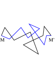
Figure 1: Two typical realizations of a monitored quantum walk on a graph from $|{\bf r}_{M^{\prime}}\rangle$ to $|{\bf r}_{M}\rangle$ with $8$ steps between projective measurement, where the links represent elements of the evolution matrix ${\hat{T}}_{M}$. The measured state $|{\bf r}_{M}\rangle$ is only visited at the end of the quantum walk. The summation with respect to all possible quantum walk realizations gives the quantum walk sum (QWS) of Eq. (5).

2 Unitary vs. monitored evolution

In the following we will calculate the transition amplitude for a quantum walk on a graph, comprising $N$ sites $\{{\bf r}_{j}\}_{j=1,\ldots,N}$ with associated states $\{|{\bf r}_{j}\rangle\}$. These states can be assumed to be single particle states but any other finite-dimensional basis is possible as well. The measured state is an element of the basis $|\psi\rangle=|{\bf r}_{M}\rangle$, and the initial state $|\psi_{0}\rangle=|{\bf r}_{M^{\prime}}\rangle$ is from the same basis. This choice will simplify the calculations but can also be generalized in a straightforward manner. The definition of the graph does not provide a structure, i.e., there is no distance. The latter will be created by the quantum walk. Then, for instance, a distance between basis states can be defined by the transition probability between different states. As we will see below, the resulting structure depends on the type of quantum walk, e.g., whether it is based on a unitary or a monitored evolution. It also depends on the eigenvectors of the evolution operator.

Although we are mostly interested in the monitored evolution, we consider the unitary evolution first. The transition amplitude reads in this case $\langle{\bf r}_{M}|e^{-iHt/\hbar}|{\bf r}_{M^{\prime}}\rangle$ with a continuous time $t$ and the Hamiltonian $H$. For the uniform state $|\psi_{0}\rangle=\sum_{k}|{\bf r}_{k}\rangle/\sqrt{N}$ we assume that it is invariant under the unitary evolution:

$$e^{-iHt/\hbar}|\psi_{0}\rangle=|\psi_{0}\rangle,$$ (1)

such that this state is eigenstate of the evolution operator with eigenvalue 1 and, consequently, an eigenstate of $H$ with zero eigenvalue. (In the following we will use the notation in which the Planck constant $\hbar$ is implicit in the definition of $H$.) Assuming further that the spectrum of $H$ is non-negative, the zero energy energy eigenvector means that the uniform state is a stationary groundstate. Moreover, Eq. (1) implies the detailed balance condition for the transition amplitude

$$\sum_{k=1}^{N}\langle{\bf r}_{j}|e^{-iHt}|{\bf r}_{k}\rangle=1\ \ \ (t\geq 0),$$ (2)

which defines a uniform eigenvector with eigenvalues 1 for the evolution matrix $(\langle{\bf r}_{j}|e^{-iHt}|{\bf r}_{k}\rangle)$, namely ${\bf v}_{1}=(1,\ldots,1)^{T}/\sqrt{N}$. The other eigenvectors of the unitary matrix $(\langle{\bf r}_{j}|e^{-iHt}|{\bf r}_{k}\rangle)$ must be orthogonal to ${\bf v}_{1}$ for non-degenerate eigenvalues. It should be noted that for a classical random walk the detailed balance condition applies to the transition probability, since there is no transition amplitude. For the unitary evolution of the quantum walk the transition probability obeys detailed balance inherently: $\sum_{k=1}^{N}\langle{\bf r}_{j}|e^{-iHt}|{\bf r}_{k}\rangle\langle{\bf r}_{k}|e^{iHt}|{\bf r}_{j}\rangle=1$.

For many practical questions regarding the unitary evolution it is convenient to average with respect to the continuous time [6]. An example is the transition probability. With eigenstates and eigenvalues of the Hamiltonian $H$, $\{|E_{k}\rangle\}$ and $\{E_{k}\}$, we define $q_{j,k}=\langle{\bf r}_{j}|E_{k}\rangle$ and $q^{*}_{j,k}=\langle E_{k}|{\bf r}_{j}\rangle$, from which we get the orthonormality relation $\sum_{k=1}^{N}q_{j,k}q_{j^{\prime}{},k}^{*}=\delta_{jj^{\prime}}$ and the time-average transition probability

$$\bar{P}_{kk^{\prime}{}}=\lim_{\epsilon\to 0}\epsilon\int_{0}^{\infty}|\langle{\bf r}_{k}|e^{-iHt}|{\bf r}_{k^{\prime}{}}\rangle|^{2}e^{-\epsilon t}dt=\sum_{j}|q_{k,j}|^{2}|q_{k^{\prime},j}|^{2},$$ (3)

where the second equation is valid for non-degenerate eigenvalues. In the case of degenerate eigenvalues we must extend the summation over $j$ to a double summation over all pairs of degenerate states. It should be noted that this expression, as a result of the time average, depends only on the spectral weights $\{q_{k,j}\}$ but not on the eigenvalues $\{E_{k}\}$.

As an alternative to the time-averaged unitary evolution, we introduce repeated measurements which provides an evolution defined at discrete measurement times [17]. Then our goal is to detect the state $|{\bf r}_{M}\rangle$ for the first time, assuming that we only measure at discrete times $\tau,2\tau,\ldots$. In this case the measurement is performed by the projector $\Pi_{M}={\bf 1}-|{\bf r}_{M}\rangle\langle{\bf r}_{M}|$ with the identity operator ${\bf 1}$. Thus, we obtain for the evolution of $|{\bf r}_{M^{\prime}{}}\rangle$ a sequence of $m-1$ measurements with $|\psi_{m}\rangle=(e^{-iH\tau}\Pi_{M})^{m-1}e^{-iH\tau}|{\bf r}_{M^{\prime}{}}\rangle$. Assuming that there exists an integer $m_{f}$ with $|\psi_{m_{f}}\rangle\propto|{\bf r}_{M}\rangle$, we get $|\psi_{m}\rangle=0$ for all $m>m_{f}$. This means that the monitored evolution of $|{\bf r}_{M^{\prime}{}}\rangle$ terminates at $m=m_{f}$, and that it is characterized by the finite sequence of transition amplitudes $\phi_{MM^{\prime}{}}(m,\tau)=\langle{\bf r}_{M}|(e^{-iH\tau}\Pi_{M})^{m-1}e^{-iH\tau}|{\bf r}_{M^{\prime}{}}\rangle$ for $1\leq m\leq m_{f}$. The existence of $m_{f}<\infty$ depends on the details of the evolution [18]. This was studied previously [17, 19] and will also be a subject of the present work.

The transition amplitude $\phi_{MM^{\prime}{}}(m,\tau)$ can be rewritten as [20]

$$\phi_{MM^{\prime}{}}(m,\tau)=\langle{\bf r}_{M}|e^{-iH\tau/2}T_{M}^{m-1}e^{-iH\tau/2}|{\bf r}_{M^{\prime}{}}\rangle\ ,\ \ T_{M}:=e^{-iH\tau/2}\Pi_{M}e^{-iH\tau/2},$$ (4)

where $T_{M}$ is the monitored evolution operator, the analogue to the unitary evolution operator $e^{-iH\tau}$ for the monitored evolution. In contrast to the unitary evolution, the monitored evolution does not obey detailed balance $\sum_{M^{\prime}=1}^{N}|\Phi_{MM^{\prime}}(m,\tau)|^{2}<1$ for $m>1$, reflecting that the projective measurement effectively couple the quantum walk to the environment. Moreover, the sum of the transition probabilities with respect to the number of measurements is restricted as $\sum_{m\geq 1}|\Phi_{MM^{\prime}}(m,\tau)|^{2}\leq 1$. This is a consequence of the fact that $\sum_{m^{\prime}=1}^{m}|\Phi_{MM^{\prime}}(m^{\prime},\tau)|^{2}$ is the probability of the transition $|{\bf r}_{M^{\prime}}\rangle\to|{\bf r}_{M}\rangle$ under the condition that $|{\bf r}_{M}\rangle$ was not measured for any $2\leq m^{\prime}\leq m$. This monitoring approach was discussed in Ref. [17] and has been applied to single-particle states to detect the particle location on a graph [21, 22, 19, 23, 24, 25, 26] as well as to spin systems [27]. Its advantage, in comparison to a unitary evolution, is that all information about the transition $|{\bf r}_{M^{\prime}{}}\rangle\to|{\bf r}_{M}\rangle$ is recorded in $m_{f}$ measurements.

The amplitude for the monitored transition in Eq. (4) can be rewritten as a quantum walk sum (QWS) (cf. App. A)

$$\phi_{MM^{\prime}}(m,\tau)=\sum_{k_{1},\ldots,k_{m}}z_{1}^{2}z_{2}^{2}\cdots z_{m}^{2}q_{M,k_{1}}K_{M;k_{1},k_{2}}\cdots K_{M;k_{m-1},k_{m}}q^{*}_{M^{\prime}{},k_{m}}$$ (5)

with $z_{k}=e^{-iE_{k}\tau/2}$. Two realizations of a QWS are visualized in Fig. 1. The matrix elements of the evolution matrix ${\hat{T}}_{M}$ and the kernel $K_{M}$ are related as

$${\hat{T}}_{M;kl}:=\langle E_{k}|T_{M}|E_{l}\rangle=z_{k}K_{M;kl}z_{l}\ \ {\rm with}\ \ K_{M;kl}:=\delta_{kl}-q_{M,k}^{*}q_{M,l}=\sum_{j\neq M}q_{j,k}^{*}q_{j,l}.$$ (6)

The last equation is a consequence of the fact that $\{|{\bf r}_{k}\rangle\}$ is a complete basis. The kernel $K_{M}$ is a projector (i.e., $K_{M}^{2}=K_{M}$) and satisfies the eigenvalue equation

$$\sum_{l=1}^{N}K_{M;kl}q^{*}_{M^{\prime},l}=(1-\delta_{MM^{\prime}})q_{M^{\prime},k}^{*}$$ (7)

with the eigenvalue $\nu_{M}=0$ for the eigenvector ${\bf Q}_{M}^{*}=(q^{*}_{M,1},\ldots,q^{*}_{M,N})^{T}$ and $N-1$ degenerate eigenvalues $\nu_{M^{\prime}}=1$ ($M^{\prime}\neq M$) for the eigenvectors ${\bf Q}_{M^{\prime}}^{*}$.

Multiplication of the kernel from both sides with the diagonal unitary matrix $D^{1/2}={\rm diag}(z_{1},\ldots,z_{N})$ distributes the eigenvalues $\{\lambda_{k}\}$ of $T_{M}$ over the entire unit disk, leaving only the zero eigenvalue $\nu_{M}$ unchanged: $\lambda_{M}=\nu_{M}=0$ . As long as $|\lambda_{k}|<1$ the corresponding eigenstates decay exponentially under the evolution with ${\hat{T}}_{M}^{m-1}$. However, in the presence of a degeneracy $z_{k}=z_{l}$ there exist also eigenvalues at the circular boundary of the disk with $|\lambda_{l}|=1$ (cf. App. B), whose eigenstates do not decay [25, 26]. We will see in the next section that energy orthogonal states have a similar effect.

3 Localized states

The definition of a localized state $|{\bf r}_{k}\rangle$ requires a reference basis. In our specific case this is the energy eigenbasis $\{|E_{j}\rangle\}$ of the Hamiltonian $H$ and the unitary evolution operator $\exp(-iH\tau)$. To understand the main features of localized states, we consider special realizations. The extreme example of a localized basis $\{|{\bf r}_{k}\rangle\}$ is the energy eigenbasis itself. In this case the measured state is also an energy eigenstate, and we get $q_{k,j}=\delta_{jk}$ for all $j,k$. Then Eq. (6) is the diagonal evolution matrix

$${\hat{T}}_{M;jk}=z_{k}^{2}\delta_{jk}(1-\delta_{Mk}).$$ (8)

From this result we get for Eq. (4) the transition amplitude $\phi_{MM^{\prime}}(1,\tau)=\delta_{MM^{\prime}{}}$ and $\phi_{MM^{\prime}}(m,\tau)=0$ for any $m\geq 2$, which is identical with the quantum Zeno limit $\tau\sim 0$ directly from Eq. (4). This is a consequence of the unitary evolution between projective measurements that changes only the phase of the initial state but does not allow any transition to other states. This is also the case for the time-average transition probability in Eq. (3), which becomes the unit matrix in this basis. In contrast, the extreme example for delocalized states are plane waves

$$q_{k,j}=\frac{1}{\sqrt{N}}e^{2\pi i(k-1)(j-1)/N},$$ (9)

which yields for the monitored evolution the matrix elements

$$\langle E_{k}|T_{M}|E_{l}\rangle=z_{k}^{2}\delta_{kl}-\frac{1}{N}e^{-2\pi i(k-l)(M-1)/N}z_{k}z_{l}.$$ (10)

When the initial state is localized to some subspace, a unitary evolution will not leave this localized space such that all states outside the localized space cannot be reached. Next it will be shown that this is different in the case of the monitored evolution.

First, we clarify what is formally understood as localization in the context of quantum walks on a finite-dimensional Hilbert space. We define a state $|{\bf r}_{k}\rangle$ as localized in terms of the energy eigenstates if the inverse participation ratio

$$c_{k}:=\sum_{j=1}^{N}|q_{k,j}|^{4}$$ (11)

does not vanish asymptotically for $N\sim\infty$. (Note that $c_{k}:=\sum_{j=1}^{N}|q_{k,j}|^{4}\neq\sum_{k=1}^{N}|q_{k,j}|^{4}$. The latter was used in Ref. [28].) In contrast, $|{\bf r}_{k}\rangle$ is delocalized when $c_{k}\sim 1/N$ for $N\sim\infty$. Thus, a localized state $|{\bf r}_{k}\rangle$ is defined by the Hamiltonian $H$ or the unitary evolution operator that has an overlap with only a few energy eigenstates $|E_{j}\rangle$. More specific, the number of overlapping states remains finite when we increase the size of the Hilbert space. While for the extremely localized example of $q_{k,j}=\delta_{jk}$ the inverse participation ratio is $c_{k}=1$ ($1\leq j\leq N$), for the plane-wave basis the inverse participation ratio is $c_{k}=1/N$ for $1\leq k\leq N$.

We note that the concept of localization can also be formulated for the unitary evolution in terms of the time averaged transition probability of Eq. (3). It refers to the correlation of two states during the evolution, namely $|{\bf r}_{k}\rangle$ and $|{\bf r}_{k^{\prime}}\rangle$, and is characterized as an exponential decay with $|{\bf r}_{k}-{\bf r}_{k^{\prime}}|$. This definition is more common in the context of quantum transport and will not be used here. It should be noted that the inverse participation ratio $c_{k}$ is the time-averaged return probability $\bar{P}_{kk}$ of the unitary evolution. The fact that $\bar{P}_{kk}\sim N^{0}$ for localized states reflects that the quantum walk returns frequently to the initial state upon time average, while $\bar{P}_{kk}\sim 1/N$ for delocalized states indicates that the return of the quantum walk to the initial state vanishes asymptotically for large systems.

The basis $\{|{\bf r}_{k}\rangle\}$ may have a state $|{\bf r}_{l}\rangle$ for a fixed $l$ that is orthogonal to the energy eigenstate $|E_{j}\rangle$ with fixed $j$: $q_{l,j}=\langle{\bf r}_{l}|E_{j}\rangle=0$. Such a state $|{\bf r}_{l}\rangle$ will be called subsequently an energy orthogonal state (EOS). An EOS corresponds to the zero charge in the charge picture of Ref. [18], where the charge is $p_{j}=|q_{M,j}|^{2}$. A localized state can be constructed from a set of EOSs, which obeys $c_{k}\sim N^{0}$. Then Eq. (6) implies with $q_{M,j}=0$ for a fixed $j$ an isolated diagonal element for the monitored evolution matrix as

$${\hat{T}}_{M;jj^{\prime}}={\hat{T}}_{M;j^{\prime}j}=z^{2}_{j}\delta_{jj^{\prime}}$$ (12)

for all $j^{\prime}$ and with the eigenvalue $z_{j}^{2}$ on the unit circle. This matrix element prevents transitions $|E_{j}\rangle\to|E_{j^{\prime}}\rangle$ as well as transitions $|E_{j^{\prime}}\rangle\to|E_{j}\rangle$, which isolates the energy eigenstate $|E_{j}\rangle$ from the evolution of the other energy eigenstates. More general, EOSs with $q_{M,j}=0$ for $j\in{\cal L}_{M}$ imply

$${\hat{T}}_{M;jj^{\prime}}=\cases{z_{j}z_{j^{\prime}}(\delta_{jj^{\prime}}-q^{*}_{M,j}q_{M,j^{\prime}})&for $j,j^{\prime}\neq{\cal L}_{M}$\cr z_{j}^{2}\delta_{jj^{\prime}}&otherwise\cr},$$ (13)

which yields with $q_{M^{\prime},j}=0$ for $j\in{\cal L}_{M^{\prime}{}}$ the monitored transition amplitude

$$\phi_{MM^{\prime}{}}(m,\tau)=\sum_{k\notin{\cal L}_{M},l\notin{\cal L}_{M}\cup{\cal L}_{M^{\prime}}}q_{M,k}z_{k}[{\hat{T}}_{M}^{m-1}]_{kl}q_{M^{\prime},l}^{*}z_{l}$$

$$=\sum_{j_{1},\ldots,j_{m-1}\notin{\cal L}_{M},j_{m}\notin{\cal L}_{M}\cup{\cal L}_{M^{\prime}}}z_{j_{1}}^{2}z_{j_{2}}^{2}\cdots z_{j_{m}}^{2}q_{M,j_{1}}(\delta_{j_{1}j_{2}}-q^{*}_{M,j_{1}}q_{M,j_{2}})\cdots(\delta_{j_{m-1}j_{m}}-q^{*}_{M,j_{m-1}}q_{M,j_{m}})q^{*}_{M^{\prime}{},j_{m}}.$$ (14)

This result corresponds with the QWS in Eq. (A) of App. A when $\sum_{k_{m}\neq M}q^{*}_{k_{m},j_{m-1}}q_{k_{m},j_{m}}$ is replaced by $\delta_{j_{m-1}j_{m}}-q^{*}_{M,j_{m-1}}q_{M,j_{m}}$ due to the completeness relation in Eq. (6). Thus, only the elements $q_{M,j}$ and $q^{*}_{M^{\prime}{},j}$ ($j=1,\ldots,N$) appear in the QWS, and $q_{M,j}=0$ for $j\in{\cal L}_{M}$ reduces the summation further due to Eq. (13). This means that we can replace ${\hat{T}}_{M}$ by the projected matrix $\Pi_{{\cal L}_{M}}{\hat{T}}_{M}\Pi_{{\cal L}_{M}}$, where $\Pi_{{\cal L}_{M}}$ projects onto the space with $j\notin{\cal L}_{M}$, in the QWS:

$$\phi_{MM^{\prime}{}}(m,\tau)=\sum_{k\notin{\cal L}_{M},l\notin{\cal L}_{M}\cup{\cal L}_{M^{\prime}}}q_{M,k}z_{k}[\Pi_{{\cal L}_{M}}{\hat{T}}_{M}\Pi_{{\cal L}_{M}}]^{m-1}_{kl}q_{M^{\prime},l}^{*}z_{l}.$$ (15)

This transition amplitude vanishes if $q_{M,j}q_{M^{\prime},j}^{*}=0$ for all $j$. Moreover, since the projection $\Pi_{{\cal L}_{M}}$ restricts the evolution to a subspace of the $N$–dimensional Hilbert space, the number of independent quantum walks is also restricted. Formally this means that we have the same evolution for different initial states $|{\bf r}_{M^{\prime}}\rangle$, $|{\bf r}_{M^{\prime\prime}}\rangle$ ($M^{\prime}\neq M^{\prime\prime}$) when the relation

$${\bf Q}_{M}\cdot\Pi_{{\cal L}_{M}}{\bf Q}_{M^{\prime}}^{*}={\bf Q}_{M}\cdot\Pi_{{\cal L}_{M}}{\bf Q}_{M^{\prime\prime}}^{*}$$ (16)

is valid.

There are several physical quantities which can be derived from the transition amplitude $\Phi_{MM^{\prime}}(m,\tau)$. Here we will focus on the transition probability $|\Phi_{MM^{\prime}}(m,\tau)|^{2}$ and the mean transition time

$${\bar{\tau}}_{{\cal N};MM^{\prime}}:=\tau\frac{\sum_{m=1}^{\cal N}(m-1)|\Phi_{MM^{\prime}{}}(m,\tau)|^{2}}{\sum_{m=1}^{\cal N}|\Phi_{MM^{\prime}{}}(m,\tau)|^{2}}$$ (17)

for at most ${\cal N}-1$ measurements. In general, the transition probability is a strongly fluctuating quantity with $0\leq|\Phi_{MM^{\prime}}(m,\tau)|^{2}\leq 1$ (cf. Fig. 3). However, for $M^{\prime}=M$ its sum is restricted as $\sum_{m\geq 1}|\Phi_{MM}(m,\tau)|^{2}=1$ for any (random) sequence of projective measurements if $m_{f}<\infty$, as shown in Ref. [29]. This means that the return probability is always 1 for sufficiently many measurements. On the other hand, for $M\neq M^{\prime}$ we have only $\sum_{m\geq 1}|\Phi_{MM^{\prime}}(m,\tau)|^{2}\leq 1$, where the actual value depends on the details of the quantum walk. For instance, in the quantum Zeno limit the probability even vanishes for the transition $|{\bf r}_{M^{\prime}{}}\rangle\to|{\bf r}_{M}\rangle$ ($M^{\prime}\neq M$). Thus, the quantum walk is characterized by the matrix structure of $|\Phi_{MM^{\prime}}(m,\tau)|^{2}$ with respect to $M$ and $M^{\prime}$, as well as by the mean transition time $\tau_{MM^{\prime}}$ for $|{\bf r}_{M^{\prime}{}}\rangle\to|{\bf r}_{M}\rangle$. This is also known as the mean first detected transition (FDT) time [18].

4 Recursive properties of the monitored evolution

A fundamental property of the unitary evolution of a closed quantum system, in contrast to classical random walks, is its non-stationary behavior [6]. The question is whether or not monitoring by repeated measurements creates stationary states? We will discuss below that there is not a unique answer to this question.

The monitored evolution is determined by the complex eigenvalues $\{\lambda_{k}\}$ of $T_{M}$, which depend on $\{q_{M,k}\}$ as well as on $\{E_{k}\}$. In particular, the decay of the evolution after $m-1$ measurements is proportional to the largest $|\lambda_{k}|^{m-1}$. As already mentioned in Sect. 2, the eigenvalues of $T_{M}$ are distributed over the complex unit disk. These eigenvalues are quite sensitive to a change of $E_{j}\tau$. As long as all eigenvalues are inside the unit disk (i.e., $|\lambda_{k}|<1$), the transition amplitude vanishes for all $m>m_{f}$ with $m_{f}<\infty$. This means that the stationary states are zero.

The situation is different when we have eigenvalues with $|\lambda_{k}|=1$. Without using the eigenvalues of $T_{M}$, we can employ the recursion relation of the transition amplitude (cf. App. C)

$$\phi_{MM^{\prime}{}}(m,\tau)=\sum_{k\neq M}\langle{\bf r}_{M}|e^{-iH\tau}|{\bf r}_{k}\rangle\phi_{kM^{\prime}{}}(m-1,\tau)$$ (18)

with $\phi_{kM^{\prime}{}}(m-1,\tau)=\langle{\bf r}_{k}|[e^{-iH\tau}({\bf 1}-|{\bf r}_{M}\rangle\langle{\bf r}_{M}|)]^{m-2}e^{-iH\tau}|{\bf r}_{M^{\prime}{}}\rangle$ and with the initial expression for $m=1$ $\phi_{MM^{\prime}{}}(1,\tau)=\langle{\bf r}_{k}|e^{-iH\tau}|{\bf r}_{M^{\prime}{}}\rangle$. An important question is whether or not there is a stationary solution ${\bar{\phi}}_{lk}$ of the recursion for $m\sim\infty$? There is always ${\bar{\phi}}_{lk}=0$, which corresponds with a decaying solution. However, as shown in App. C.1, a nonzero solution exists when there is a $k$ with (i) an EOS $q_{M,k}=0$ and (ii) $z_{k}^{2}=1$. Condition (i) implies ${\hat{T}}_{M;kl}={\hat{T}}_{M;lk}=\delta_{lk}$ for all $l$, which corresponds with Eq. (12). Condition (ii) means the restriction of the energy eigenvalue to $E_{k}\tau=0\ ({\rm mod}\ 2\pi)$. For other energy values the application of ${\hat{T}}_{M}$ leads to a rotation $z_{k}^{m-1}$ on the complex unit circle. This is not stationary but represents a limit cycle. Thus, non-vanishing stationary solutions exist but they are isolated in the evolution.

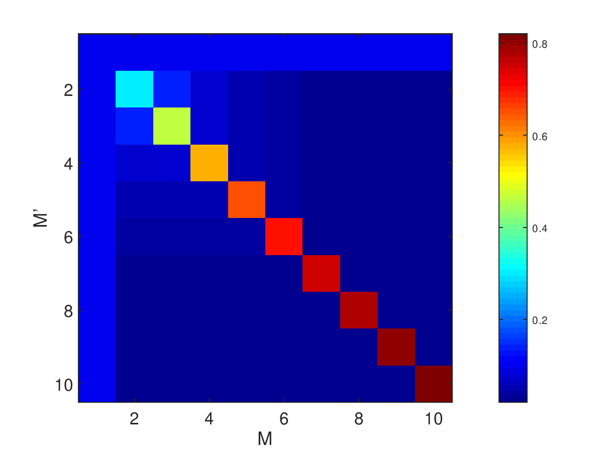
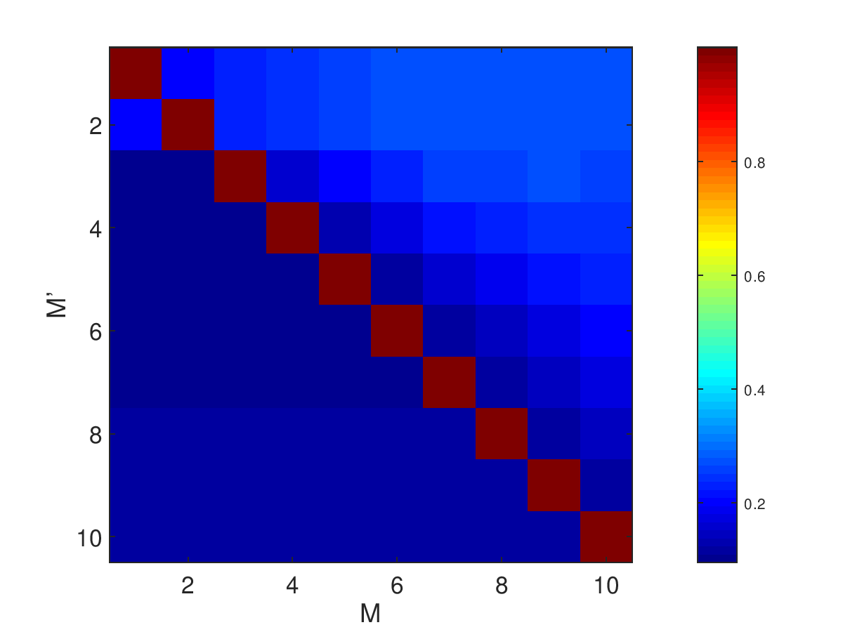
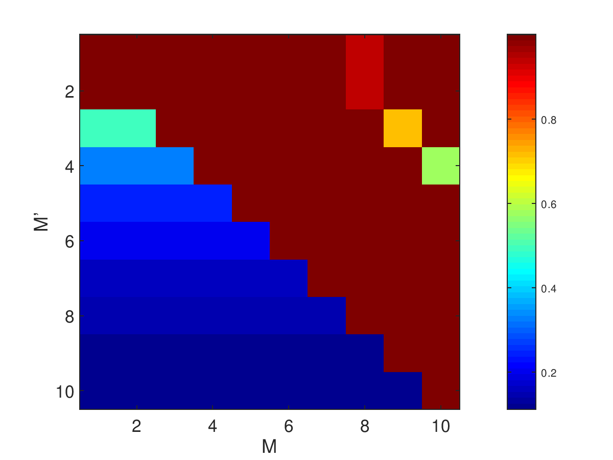
a) b) c) d)

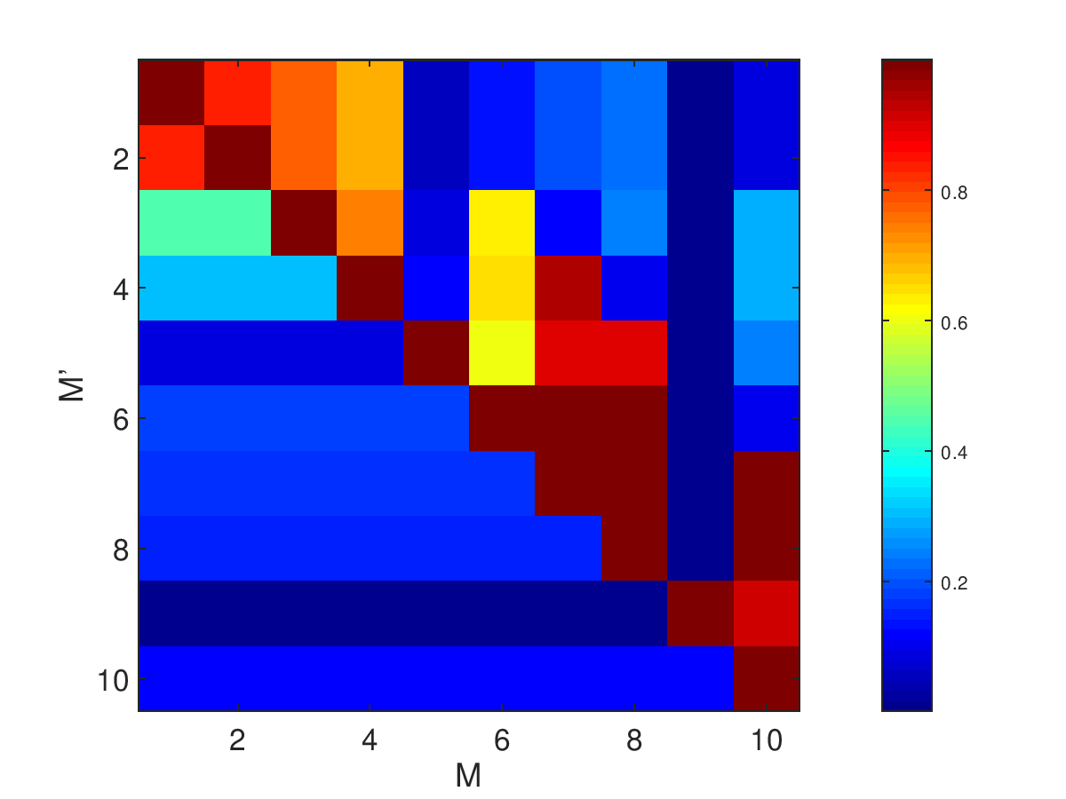
Figure 2: Transition probabilities on a graph with $N=10$ sites in the localized basis of Eq. (19). The calculation was performed for the linear spectrum $E_{k}=J(k-1)$ ($k=1,\ldots,N$). This is also the case in the other examples of Figs. 3 – 6. a) The unitary evolution of the time-averaged transition probability ${\bar{P}}_{MM^{\prime}}$ of Eq. (25) indicates a typical localization effect. b) For the monitored evolution the sum $\sum_{m=1}^{500}|\phi_{MM^{\prime}}(m,\tau)|^{2}$ reflects the quantum Zeno effect in b) for $J\tau=0.04\hbar$, while in c) for $J\tau=\hbar$ and in d) for $J\tau=\pi\hbar/2$ an asymmetric transition is visible.

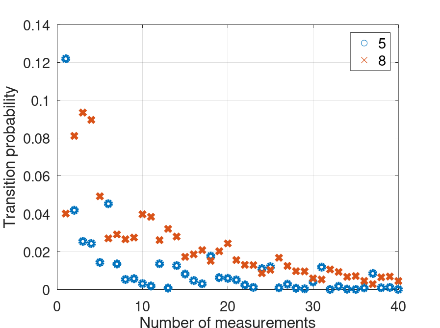
a) b)

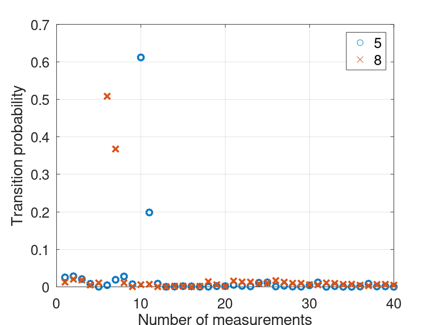
Figure 3: Transition probabilities for $|{\bf r}_{j}\rangle\to|{\bf r}_{5}\rangle$ with $J\tau=\hbar$ as a function of the number of measurements a) in the localized basis and b) in the plane-wave basis.

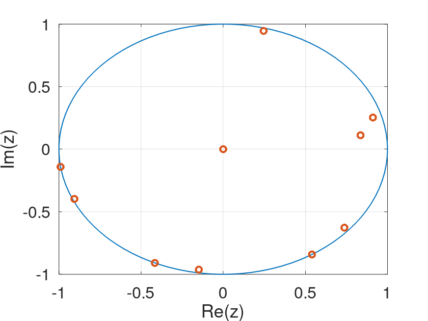
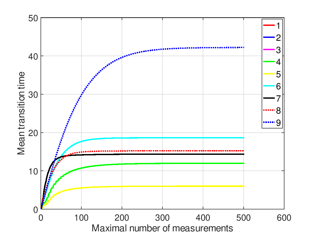
a) b)
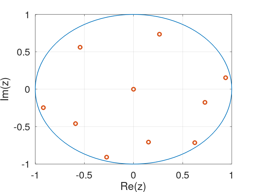
c) d)

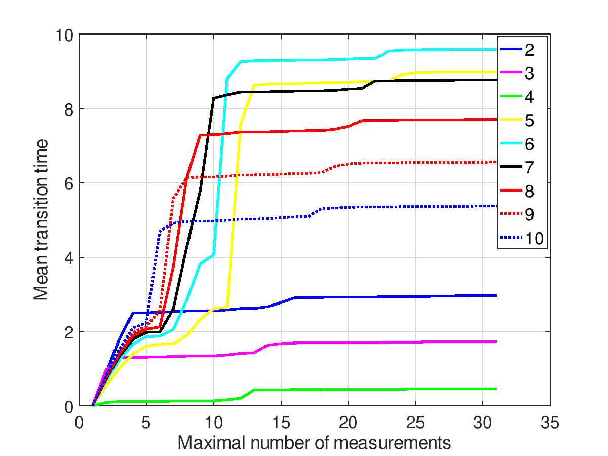
Figure 4: Eigenvalues of the monitored evolution matrix ${\hat{T}}_{5}$ for a) the localized basis and b) the plane-wave basis with $J\tau=\hbar$. The mean transition times for ${\hat{T}}_{5}$ are plotted c) in the localized basis, where $j=1,2,3,4$ are equal, and d) in the plane-wave basis.

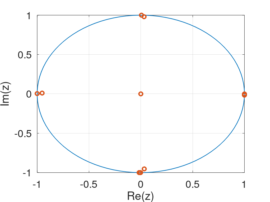
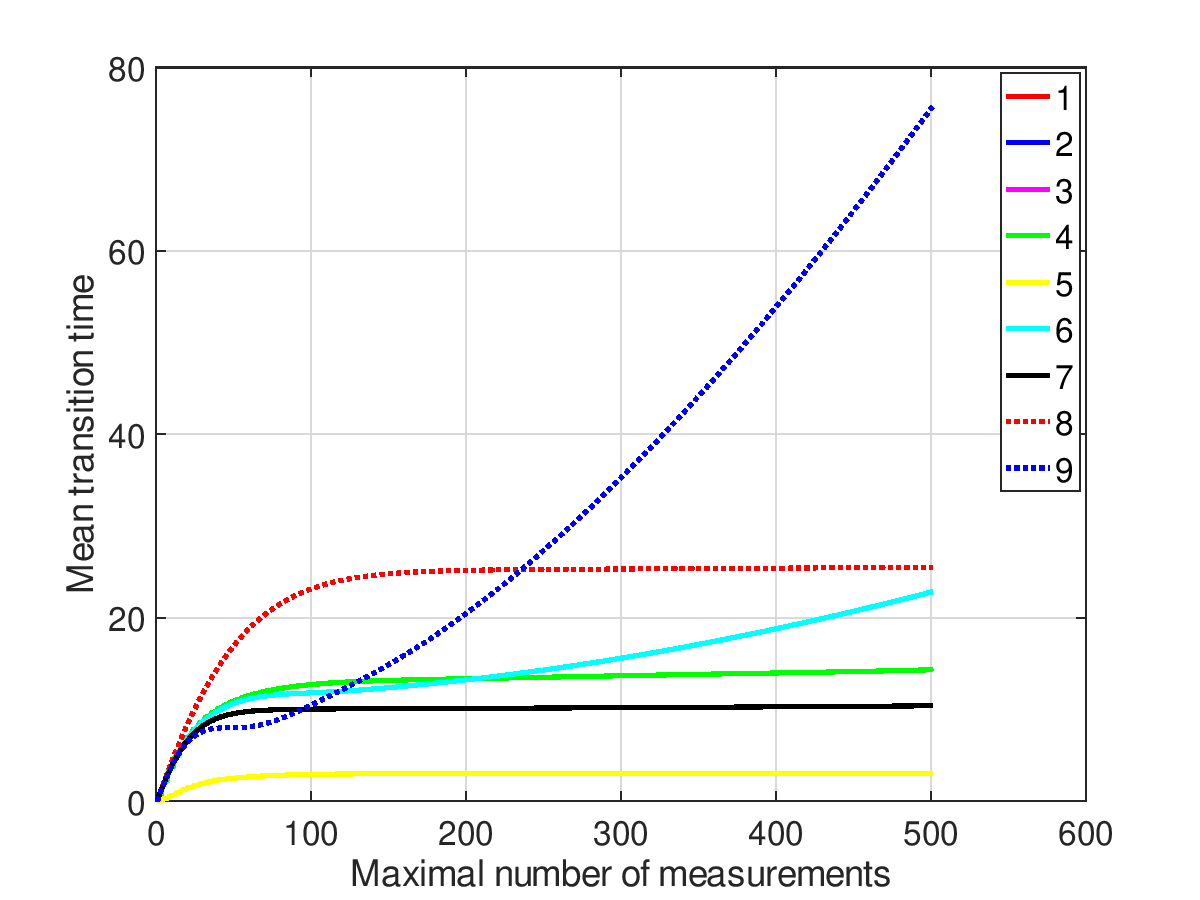
a) b)
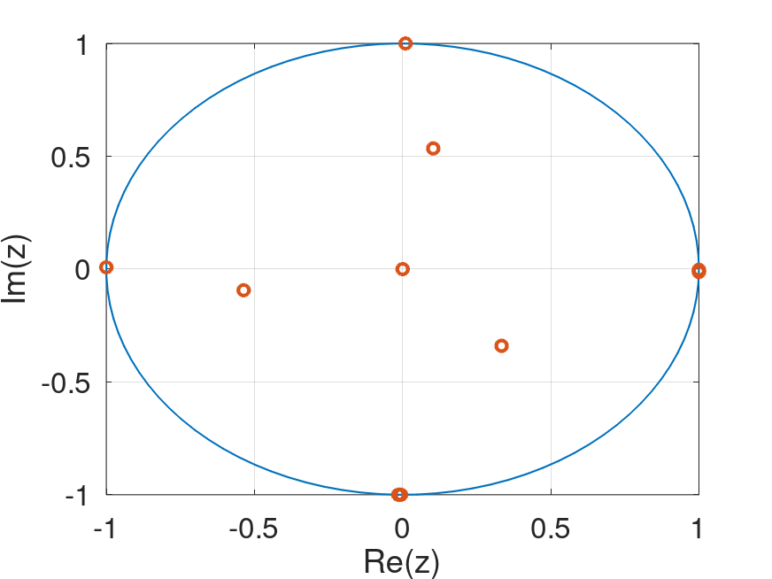
c) d)

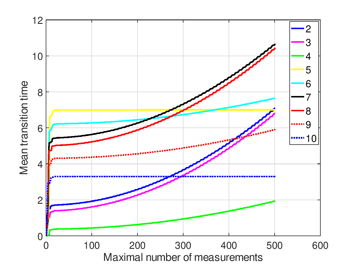
Figure 5: Eigenvalues of the monitored evolution matrix ${\hat{T}}_{5}$ with $J\tau=(\pi/2+0.002)\hbar$ a) in the localized basis and b) in the plane-wave basis. The mean transition times $|{\bf r}_{j}\rangle\to|{\bf r}_{5}\rangle$ are plotted c) in the localized basis and d) in the plane-wave basis. They diverge for some transitions due to the vicinity of spectral degeneracies.

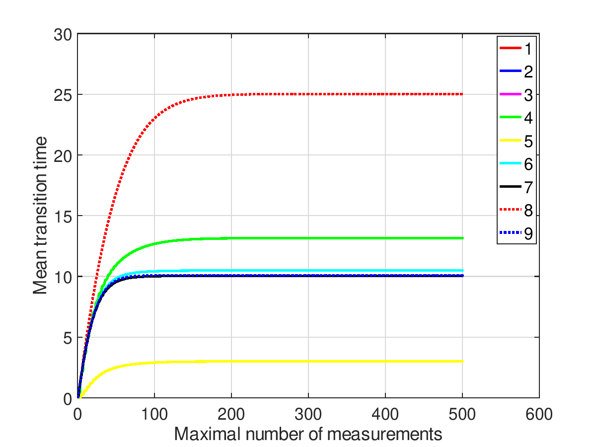
a) b)

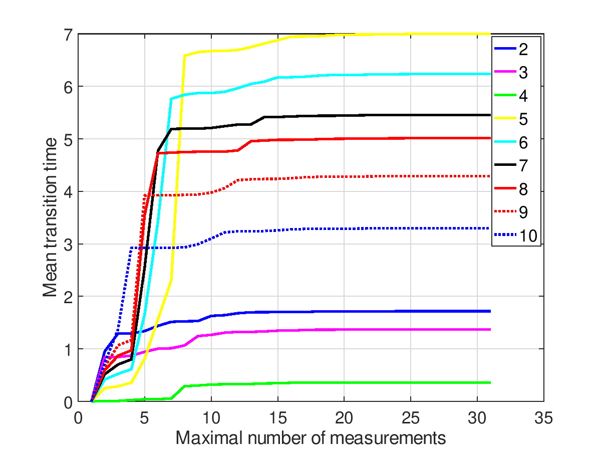
Figure 6: Mean transition time $|{\bf r}_{j}\rangle\to|{\bf r}_{5}\rangle$ with $J\tau=\pi\hbar/2$ a) in the localized basis, where $j=1,2,3,4$ and $j=7,9$ are equal and b) in the plane-wave basis.

5 Discussion and examples

In Sects. 2 and 3 we have found that degenerate eigenvalues of the unitary evolution operator $\exp(-iH\tau)$ and EOSs create eigenvalues of the monitored evolution matrix ${\hat{T}}_{M}$ on the unit circle. In particular, if the measured state $|{\bf r}_{M}\rangle$ is orthogonal to $n$ energy eigenstates, the corresponding eigenvalues $\lambda_{j}$ of the monitored evolution matrix ${\hat{T}}_{M}$ obey $|\lambda_{j}|=1$. These results are in agreement with previous calculations based on the classical electrostatic picture and indicate that the poles of the electrostatic potential correspond with the eigenvalues of ${\hat{T}}_{M}$. For instance, it is known that near a spectral degeneracy or in the presence of an EOS one or more poles of the electrostatic potenial move towards the unit circle [24, 30, 31]. The connection of the poles and the eigenvalues originates in the sum $G(z)=\sum_{m\geq 1}[{\hat{T}}_{M}/z]^{m-1}=z(z{\bf 1}-{\hat{T}}_{M})^{-1}$, since the poles of $G(z)$ are the eigenvalues of ${\hat{T}}_{M}$.

The results for the transition amplitude can be used to calculate the transition probability of the unitary evolution ${\bar{P}}_{kk^{\prime}}$ of Eq. (3) as well as the monitored transition probability $|\phi_{MM^{\prime}}(m,\tau)|^{2}$ obtained from Eq. (15). Then the mean transition time ${\bar{\tau}}_{{\cal N};MM^{\prime}}$ of Eq. (17) can be calculated as for specific examples. Since $\phi_{MM^{\prime}{}}(m,\tau)=0$ for $m>m_{f}$, this expression saturates when ${\cal N}$ approaches $m_{f}$. We will focus here on a specific localized basis and plane waves as a delocalized basis to reveal some properties which distinguish these two cases. In order to obtain a robust result for the mean transition time we need a sufficiently large number of measurements ${\cal N}$, whose value depends essentially on the eigenvalues of $T_{M}$. The smaller their absolute value is, the faster the transition probability $|\phi_{MM^{\prime}{}}(m,\tau)|^{2}$ decays with $m$. Near spectral degeneracies $m_{f}$ can become arbitrarily large, which means that ${\cal N}$ needs to be very large for reliable results of the mean transition time. To demonstrate these effects we consider the linear spectrum $E_{k}=J(k-1)$, which yields a spectral degeneracy for the evolution when $(E_{k}-E_{l})\tau=J\tau(k-l)$ is a multiple of $2\pi\hbar$.

Next, we define a specific basis, namely a basis with a single delocalized vector ${\bf q}_{1}$, which always exists due to detailed balance according to Eq. (2), and orthogonal localized vectors ${\bf q}_{k}=(q_{1,k},\ldots,q_{N,k})^{T}$ with (cf. App. D)

$$q_{M,1}=1/\sqrt{N},\ \ q_{M,k}=\frac{1}{\sqrt{k(k-1)}}\cases{0&$1<k<M\leq N$\cr-k+1&$1<k=M\leq N$\cr 1&$1\leq M<k\leq N$\cr},$$ (19)

where $\{{\bf q}_{1},\ldots,{\bf q}_{N}\}$ forms an orthonormal basis. This basis is inspired by an eigenbasis of the Hamiltonian that connects all $N$ vertices of a graph with equal weights [28].

The delocalized vector ${\bf v}_{1}$ gives $c_{1}=1/N$, while the other vectors ${\bf q}_{k}$ ($2\leq k\leq N$) are localized with the inverse participation ratio

$$c_{k}=\frac{1}{N^{2}}+(1-1/k)^{2}+\sum_{j=k+1}^{N}\frac{1}{j^{2}(j-1)^{2}}$$ (20)

with the right-hand side bounded from below by $1/4$ for any $N$. Within this basis an energy eigenstate is expressed in the basis $\{|{\bf r}_{k}\rangle\}$ as $|E_{j}\rangle=\sum_{k}q_{k,j}|{\bf r}_{k}\rangle$ with

$$|E_{1}\rangle=\frac{1}{\sqrt{N}}\sum_{k=1}^{N}|{\bf r}_{k}\rangle\ ,\ |E_{j}\rangle=-\sqrt{1-1/j}|{\bf r}_{j}\rangle+\frac{1}{\sqrt{j(j-1)}}\sum_{k=1}^{j-1}|{\bf r}_{k}\rangle\ \ (2\leq j\leq N),$$ (21)

where $|E_{1}\rangle$ is delocalized on the graph and $|E_{j}\rangle$ ($2\leq j\leq N$) is localized at $|{\bf r}_{j}\rangle$.

5.1 Strong localization

For the basis defined in Eq. (19) the strongest localization effect on the QWS exists for $M=N$, where the summation in Eq. (3) is reduced to $j_{m}=1,N$ with $q_{N,1}=1/\sqrt{N}$ and $q_{N,N}=\sqrt{1-1/N}$. This represents an effective two-level system with transitions between $|{\bf r}_{1}\rangle$ and $|{\bf r}_{N}\rangle$, whose projected evolution matrix reads

$$\Pi_{{\cal L}_{N}}{\hat{T}}_{N}\Pi_{{\cal L}_{N}}=\frac{1}{N}\pmatrix{N-1&z_{N}\sqrt{N-1}\cr z_{N}\sqrt{N-1}&z_{N}^{2}\cr}$$ (22)

with eigenvalues $\lambda_{1}=0$ and $\lambda_{2}=(z_{N}^{2}+N-1)/N$. The decay of the transition amplitude is determined by $|\lambda_{2}|^{2}=(1-1/N)^{2}+1/N^{2}+2(1-1/N)\cos(E_{N}\tau)/N$, which decreases with increasing $N$. The asymptotic behavior scales with $N$ as

$$|\lambda_{2}|^{m-1}=\exp\left\{-\frac{m-1}{N}\left[1-\cos(E_{N}\tau)\right]+O(N^{-2})\right\}.$$ (23)

The transition amplitude $\phi_{MM^{\prime}}(m,\tau)$ also depends on $q_{M^{\prime},j}$, where $q_{M^{\prime},1}=1/\sqrt{N}$ and

$$q_{M^{\prime},N}=\cases{1/\sqrt{N(N-1)}&for $M^{\prime}<N$\cr-\sqrt{1-1/N}&for $M^{\prime}=N$\cr}$$ (24)

contribute to $M=N$. Thus, for large $N$ the amplitude for the transition $|{\bf r}_{N}\rangle\to|{\bf r}_{N}\rangle$ is of order 1, whereas the amplitudes of other transitions are at most of order $1/N$.

5.2 Transition probability for the unitary evolution

First, we consider the unitary evolution for the basis defined in Eq. (19) and calculate the right-hand side of Eq. (3):

$${\bar{P}}_{1k^{\prime}{}}={\bar{P}}_{k1}=\frac{1}{N},$$

which means that the transition probability from or to the state $|{\bf r}_{1}\rangle$ is equal $1/N$. This case is special because $k=1$ or $k^{\prime}{}=1$ refer to the uniformly delocalized eigenvector ${\bf v}_{1}$ due to the detailed balance condition in Eq. (2). In contrast, for the localized states with $2\leq k,l\leq N$ the transition probability ${\bar{P}}_{kl}$ decays with increasing $k$ and $l$. Since ${\bar{P}}_{kl}$ is symmetric, we can assume without restriction that $l\geq k$. Then we get

$${\bar{P}}_{kl}=\sum_{j=1}^{N}|q_{k,j}|^{2}|q_{l,j}|^{2}=\frac{1}{N^{2}}+\frac{1}{l^{2}}+\sum_{j=l+1}^{N}\frac{1}{j^{2}(j-1)^{2}}\ \ (2\leq k<l<N),\ \ \ {\bar{P}}_{kN}=\frac{2}{N^{2}}\ \ (2\leq k<N).$$ (25)

In contrast, for the plane-wave basis of Eq. (9) there is no decay with $l$ but ${\bar{P}}_{kl}=1/N$. Thus, the transition between any pair of states on the graph has the same probability $1/N$ after time average.

5.3 Examples for a graph of dimension $N=10$

In Figs. 2 – 6 we visualize some results of a quantum walk on a graph with $N=10$ sites and with matrix elements $H_{kl}=J\sum_{j=1}^{10}q_{k,j}(j-1)q_{l,j}^{*}$ of the Hamiltonian $H$ in the basis $\{|{\bf r}_{k}\rangle\}$. The localization effect on the spatial structure of the transition probability is illustrated for the unitary evolution in Fig. 2a and for the monitored evolution in Fig. 2b-c. Fig. 2a visualizes the typical localization effect with a monotonic decay of ${\bar{P}}_{kl}$ with the distance $|k-l|$. On the other hand, the behavior of the monitored transition probability $\sum_{m=1}^{500}|\phi_{MM^{\prime}}(m,\tau)|^{2}$ is more complex and depends strongly on the parameter $J\tau$. For instance, it is similar to the unitary evolution for small $J\tau$ due to the quantum Zeno effect (Fig. 2b). This means that the system remains near the initial state due to frequent measurements. For $J\tau=\hbar$ the transition probability is flat for $M^{\prime}<M$ at a value less than $1$, typically of order $1/N$, and jumps to 1 for $M^{\prime}\geq M$ (Fig. 2b). For $J\tau=\pi\hbar/2$ it is smaller than 1 away from the line $M^{\prime}=M$ in Fig. 2d. All three cases have in common that the monitored transition probability is 1 if $M^{\prime}=M$, which reflects that the return probability is always 1. The triangular structure is caused by the vanishing projected evolution matrix elements $[\Pi_{{\cal L}_{M}}{\hat{T}}_{M}\Pi_{{\cal L}_{M}}]_{kl}=0$ for $2\leq k,l<M$ and $q_{M^{\prime},l}=0$ for $2\leq l<M^{\prime}$.

The quantum walks on the localized basis provide a structure of the graph with connections between the vertex states $\{|{\bf r}_{k}\rangle\}$ through the transition probabilities. While the unitary evolution creates symmetric transitions in Fig. 2a, the monitored evolution creates asymmetric transitions in Fig. 2b-c such that the quantum walk on the graph is directed. The asymmetry is very weak in the quantum Zeno regime of Fig. 2b, regardless if a localized or a plane-wave basis is used. Here only the result of the localized basis is plotted but it is very similar for the plane-wave basis. With less frequent measurements in Figs. 2c,d the asymmetry becomes stronger. In general, the complex behavior is the result of the competition between localization and measurements. This is also reflected by the irregular behavior of the transition probability $|\phi_{MM^{\prime}{}}(m,\tau)|^{2}$ as a function of the number of measurements $m$ in Fig. 3a.

Finally, we analyze the mean transition time of the monitored evolution of Eq. (17) for parameter values (i) $J\tau=\hbar$, which has no degeneracy, while for (ii) $(\pi/2+0.002)\hbar$ we are very close to multiple degeneracies of $E_{k}$. This is compared with the behavior for (iii) exactly at the degeneracies $J\tau=\pi\hbar/2$. The eigenvalues $\{\nu_{j}\}$ of the monitored transition matrix ${\hat{T}}_{M}$ are plotted in Fig. 4a for case (i) with the localized as well as with the plane-wave basis. The corresponding eigenvalues for case (ii) are plotted in Fig. 5a. In both cases the typical eigenvalues are closer to the unit circle for the localized states. Moreover, the tendency to degenerate is stronger for the eigenvalues of case (ii). A few examples for the transition probabilities in Fig. 3 illustrate that their distributions with respect to the number of measurements is broader and smoother for the localized basis.

The mean transition time for the transitions $|{\bf r}_{M^{\prime}{}}\rangle\to|{\bf r}_{M}\rangle$ as a function of the maximal number of measurements ${\cal N}$, defined in Eq. (17), is plotted in Fig. 4c,d for the case (i) and in Fig. 5c,d for the case (ii). For the localized basis the shortest mean transition time appears for the return transition $|{\bf r}_{5}\rangle\to|{\bf r}_{5}\rangle$ in Fig. 4c as well as in Figs. 5c, 6a, which is always an integer due to the protected winding number of the return [17, 18, 29]. Moreover, the curves of the mean transition times are equal for $|{\bf r}_{1,2,3,4}\rangle\to|{\bf r}_{5}\rangle$ in Figs. 4c, 5c, 6a, as a consequence of the relation in Eq. (16), and they are equal in Fig. 6a for $|{\bf r}_{7,9}\rangle\to|{\bf r}_{5}\rangle$ as a consequence of $E_{7}\tau=3\pi\hbar$ and $E_{9}\tau=4\pi\hbar$. This is different for the plane-wave basis, where the shortest mean transition time appears for the transition $|{\bf r}_{4}\rangle\to|{\bf r}_{5}\rangle$ in Figs. 4d, 5d and 6b. This behavior reflects the localization effect on the mean transition time. The vicinity of degeneracies in case (ii) leads to an increasing mean transition time for several transitions, as visualized in Fig. 5c,d. Remarkably, the diverging mean transition times do not appear exactly at the degeneracy point, as demonstrated in Fig. 6. The mean transition time is typically shorter for the plane-wave basis, indicating that the localized states prevents the quantum walk to perform the transition directly.

The behavior of the mean transition time with respect to the maximal number of measurements ${\cal N}$ is much smoother for the localized basis than for the plane-wave basis, where the latter jumps in steps (cf. Figs. 4b and 6b). This indicates that the transition probability $|\phi_{MM^{\prime}{}}(m,\tau)|^{2}$ does not decay smoothly with $m$ but has large contributions for certain values of $m$ (cf. Fig. 3b). On the other hand, Fig. 3a illustrates that it requires more measurements to reach $m_{f}$ in the localized basis.

6 Conclusions

Our approach to the monitored evolution on a graph with basis $\{|{\bf r}_{k}\rangle\}$ can be summarized as the mapping from energy levels $\{E_{j}\}$ and spectral weights $\{q_{k,j}\equiv\langle{\bf r}_{k}|E_{j}\rangle\}$ to the monitored evolution matrix ${\hat{T}}_{M}$ as $\{E_{j},q_{k,j}\}_{k,j=1,\ldots N}\to{\hat{T}}_{M}$. The corresponding unitary evolution is defined by the unitary evolution matrix $\sum_{j}e^{-iE_{j}t}q_{k,j}q^{*}_{l,j}$ for the transition $|{\bf r}_{l}\rangle\to|{\bf r}_{k}\rangle$ during the time $t$. This enabled us to calculate the transition probabilities and the mean transition times.

Localization is defined through the inverse participation ratio, which is identified in the unitary evolution by the time-averaged return probability ${\bar{P}}_{kk}$. In particular, localized states are created by $q_{M,j}=0$ for $j\in{\cal L}_{M}$. Then only the evolution matrix projected onto $j\notin{\cal L}_{M}$ provides the effective monitored evolution. The monitored evolution represents directed quantum walks on the graph through asymmetric transition probabilities. In contrast, the unitary evolution has always symmetric transition probabilities. Localized states as well as a degeneracy $(E_{k}-E_{l})\tau=0\ ({\rm mod}\ 2\pi)$ create eigenstates of the monitored evolution matrix ${\hat{T}}_{M}$ whose eigenvalues are on the unit circle.

The mean transition time enables us to distinguish between a localized and delocalized basis. In our examples we have observed that a localized basis, in comparison to a delocalized basis, has substantially larger mean transition times, implying that $m_{f}$ is typically smaller for the plane-wave basis. Moreover, a localized basis favors a quicker return to the initial state in comparison with any transition to other states. Moreover, the reduction of the Hilbert space by localization may lead to identical mean transition times for different transitions.

The competition of localization and projective measurements makes the monitored transition probability quite sensitive to changes of the spectral parameter $J\tau$. This is also reflected by the location of the eigenvalues of ${\hat{T}}_{M}$ on the complex unit disk. Since the distribution of these eigenvalues depend on the chosen basis, it would be interesting to determine their correlation in a quantative way, similar to the eigenvalue correlation in the random matrix theory [32, 33, 34].

Acknowledgment

I am grateful to Eli Barkei, Quancheng Liu and Sabine Tornow for enlightening discussions.

Appendix A Monitored evolution

Starting from the expression in Eq. (4) we can write with $\Pi_{M}={\bf 1}-|{\bf r}_{M}\rangle\langle{\bf r}_{M}|$ for the monitored transition amplitude

$$\phi_{MM^{\prime}{}}(m,\tau)=\langle{\bf r}_{M}|e^{-iH\tau}\left(\Pi_{M}e^{-iH\tau}\right)^{m-1}|{\bf r}_{M^{\prime}{}}\rangle$$

$$=\sum_{k_{1},k_{2},\ldots,k_{m-1}\neq M}\langle{\bf r}_{M}|e^{-iH\tau}|{\bf r}_{k_{1}}\rangle\langle{\bf r}_{k_{1}}|e^{-iH\tau}|{\bf r}_{k_{2}}\rangle\cdots\langle{\bf r}_{k_{m-1}}|e^{-iH\tau}|{\bf r}_{M^{\prime}{}}\rangle$$

$$=\sum_{k_{1},k_{2},\ldots,k_{m-1}\neq M}\sum_{j_{1},j_{2},\ldots,j_{m}}e^{-i(E_{j_{1}}+E_{j_{2}}+\cdots+E_{j_{m}})\tau}q_{M,j_{1}}q^{*}_{k_{1},j_{1}}q_{k_{1},j_{2}}q^{*}_{k_{2},j_{2}}\cdots q_{k_{m-1},j_{m}}q^{*}_{M^{\prime}{},j_{m}}.$$ (26)

After reordering the summations we get

$$\phi_{MM^{\prime}{}}(m,\tau)=\sum_{j_{1},j_{2},\ldots,j_{m}}e^{-i(E_{j_{1}}+E_{j_{2}}+\cdots+E_{j_{m}})\tau}q_{M,j_{1}}K_{j_{1},j_{2}}\cdots K_{j_{m-1},j_{m}}q^{*}_{M^{\prime}{},j_{m}}$$

with

$$K_{j_{l},j_{l+1}}:=\sum_{k_{l}\neq M}q^{*}_{k_{l},j_{l}}q_{k_{l},j_{l+1}}=\delta_{j_{l},j_{l+1}}-q^{*}_{M,j_{l}}q_{M,j_{l+1}},$$ (27)

which is the kernel defined already in Eq. (6). This expression is reminiscent of a functional integral [35, 36]. But instead of an integration we have a summation here with discrete time steps $\tau$. Therefore, we will call it a quantum walk sum, which is much easier to calculate than Feynman’s path integral, especially when we employ numerical methods. With this representation of the monitored transition amplitude the effect of the energy orthogonal states $|{\bf r}_{k}\rangle$ with $q_{k,j}=0$ is directly visible, since these states reduce the summation with respect to energy states $\{E_{j}\}$ with $q_{k,j}\neq 0$.

Appendix B Degeneracy and eigenvectors of the evolution

The eigenvalue equation (7) implies the relation

$$\sum_{l}{\hat{T}}_{M;kl}q^{*}_{M^{\prime},l}=(1-\delta_{MM^{\prime}})z_{k}^{2}q^{*}_{M^{\prime},k}\ \ {\rm with}\ \ q^{*}_{M^{\prime},l}=z_{l}^{*}q_{M^{\prime},l}^{*},$$ (28)

where $\{{\bf Q}_{M}\}$ with ${\bf Q}_{M}=(q_{M,1},\ldots,q_{M,N})^{T}$ is an orthonormal basis: $\sum_{k}q_{M,k}q^{*}_{M^{\prime},k}=\delta_{MM^{\prime}}$. Thus, the mapping of the vector ${\bf Q}^{*}_{M^{\prime}{}}$ ($M^{\prime}{}\neq M$) by $T_{M}$ is unitary and, therefore, does not change the length of ${\bf Q}^{*}_{M^{\prime}{}}$. In other words, we have ${\hat{T}}_{M}{\bf Q}^{*}_{M^{\prime}{}}=D{\bf Q}^{*}_{M^{\prime}{}}$ for all $M^{\prime}{}\neq M$, which is degenerated with respect to $M^{\prime}{}$, such that any linear combination of $\{{\bf Q}^{*}_{M^{\prime}}\}$ satisfies the same equation. Introducing the Cartesian vector ${\bf e}_{k}=(\langle E_{1}|E_{k}\rangle,\ldots,\langle E_{N}|E_{k}\rangle)^{T}$ and assuming that $z_{j}=z_{k}$, we can define a linear combination for $\{{\bf Q}^{*}_{M^{\prime}}\}_{M^{\prime}{}\neq M}$ that is (i) proportional to $\alpha{\bf e}_{j}+\beta{\bf e}_{k}$ and (ii) it is orthogonal to ${\bf Q}^{*}_{M}$. It is sufficient to determine the coefficients $\alpha$, $\beta$ such that they satisfy condition (ii). With the Cartesian vector ${\bf e}_{j}$ and the vector ${\bf Q}^{*}_{k}$ of Eq. (28) we get ${\bf e}_{j}\cdot{\bf Q}^{*}_{k}=z_{j}^{*}q^{*}_{k,j}$ and

$$(\alpha{\bf e}_{j}+\beta{\bf e}_{k})\cdot{\bf Q}^{*}_{M}=\alpha z_{j}^{*}q^{*}_{M,j}+\beta z_{k}^{*}q^{*}_{M,k},$$

which vanishes for $\alpha=-\beta z_{k}^{*}q^{*}_{M,k}/z_{j}^{*}q^{*}_{M,j}$, provided that $z_{j}^{*}q^{*}_{M,j}\neq 0$. This means that $\alpha{\bf e}_{j}+\beta{\bf e}_{k}$ lives in the space orthogonal to ${\bf Q}^{*}_{M}$. Thus, the degeneracy $z_{j}=z_{k}$ implies the eigenvalue equation for ${\hat{T}}_{M}$

$${\hat{T}}_{M}(\alpha{\bf e}_{j}+\beta{\bf e}_{k})=z_{k}^{2}(\alpha{\bf e}_{j}+\beta{\bf e}_{k})$$ (29)

with eigenvalue $z_{k}^{2}$, where $\alpha{\bf e}_{j}+\beta{\bf e}_{k}$ lives by definition in the space orthogonal to ${\bf Q}^{*}_{M}$. This means that this eigenvector does not decay with the number of measurements in the monitored evolution. The same argument can be applied to the case with more than two degenerate $z_{j}$. Thus, degeneracies in terms of $E_{k}\tau\ ({\rm mod}\ 2\pi)$ have a strong effect on the quantum walk by creating eigenstates of ${\hat{T}}_{M}$ with eigenvalues on the unit circle.

Appendix C Recursion relation

The monitored transition amplitude of Eq. (A) reads

$$\langle{\bf r}_{M}|e^{-iH\tau}[({\bf 1}-|{\bf r}_{M}\rangle\langle{\bf r}_{M}|)e^{-iH\tau}]^{m-1}|{\bf r}_{M^{\prime}{}}\rangle$$

$$=\langle{\bf r}_{M}|e^{-2iH\tau}[({\bf 1}-|{\bf r}_{M}\rangle\langle{\bf r}_{M}|)e^{-iH\tau}]^{m-2}|{\bf r}_{M^{\prime}{}}\rangle-\langle{\bf r}_{M}|e^{-iH\tau}|{\bf r}_{M}\rangle\langle{\bf r}_{M}|e^{-iH\tau}[({\bf 1}-|{\bf r}_{M}\rangle\langle{\bf r}_{M}|)e^{-iH\tau}]^{m-2}|{\bf r}_{M^{\prime}{}}\rangle$$

$$=\sum_{k\neq M}\langle{\bf r}_{M}|e^{-iH\tau}|{\bf r}_{k}\rangle\langle{\bf r}_{k}|e^{-iH\tau}[({\bf 1}-|{\bf r}_{M}\rangle\langle{\bf r}_{M}|)e^{-iH\tau}]^{m-2}|{\bf r}_{M^{\prime}{}}\rangle,$$

which also reads

$$\phi_{MM^{\prime}{}}(m,\tau)=\sum_{k\neq M}\langle{\bf r}_{M}|e^{-iH\tau}|{\bf r}_{k}\rangle\phi_{kM^{\prime}{}}(m-1,\tau)$$ (30)

with $\phi_{kM^{\prime}{}}(m-1,\tau)=\langle{\bf r}_{k}|e^{-iH\tau}[({\bf 1}-|{\bf r}_{M}\rangle\langle{\bf r}_{M}|)e^{-iH\tau}]^{m-2}|{\bf r}_{M^{\prime}{}}\rangle$. For $m=2$ this yields

$$\phi_{MM^{\prime}{}}(2,\tau)=\sum_{k\neq M}\langle{\bf r}_{M}|e^{-iH\tau}|{\bf r}_{k}\rangle\langle{\bf r}_{k}|e^{-iH\tau}|{\bf r}_{M^{\prime}{}}\rangle.$$

C.1 Stationary solution

A stationary solution of Eq. (18) would obey the equation

$$\sum_{l^{\prime}{}}\left[\delta_{ll^{\prime}{}}-\langle{\bf r}_{l}|e^{-iH\tau}|{\bf r}_{l^{\prime}{}}\rangle(1-\delta_{l^{\prime}{}M})\right]{\bar{\phi}}_{l^{\prime}{}k}=0.$$ (31)

This equation is solved either by ${\bar{\phi}}_{l^{\prime}{}k}=0$, which corresponds with a decaying transition amplitude, or if $({\bar{\phi}}_{1k},\ldots,{\bar{\phi}}_{Nk})^{T}$ is an eigenvector with zero eigenvalue. When we expand this vector in the Cartesian basis as $\sum_{l}{\bar{\phi}}_{lk}{\bf e}_{l}$, we get

$${\bar{\phi}}_{Mk}{\bf e}_{M}+({\bf 1}-U)\sum_{l\neq M}{\bar{\phi}}_{lk}{\bf e}_{l}=0\ ,\ \ \ U_{ll^{\prime}{}}=\langle{\bf r}_{l}|e^{-iH\tau}|{\bf r}_{l^{\prime}{}}\rangle=\sum_{j}z^{2}_{j}q_{l,j}q^{*}_{l^{\prime}{},j}.$$ (32)

A solution is ${\bar{\phi}}_{Mk}=0$ and ${\bf 1}-U$ must have a vanishing eigenvalue. Moreover, the corresponding eigenvector must be of the form $\sum_{k\neq M}\alpha_{k}{\bf e}_{k}$ with appropriate coefficients $\{\alpha_{k}$}. After replacing $({\bar{\phi}}_{1k},\ldots,{\bar{\phi}}_{Nk})^{T}\to(q_{1,k},\ldots,q_{N,k})^{T}$ we get from Eq. (32) the relation

$$\sum_{j}\left(\delta_{lj}-\sum_{l^{\prime}{}}q_{l,l^{\prime}{}}z^{2}_{l^{\prime}{}}q^{*}_{j,l^{\prime}{}}\right)q_{j,k}=(1-z_{k}^{2})q_{l,k},$$ (33)

which vanishes for a $z_{k}^{2}=1$. In the latter case we have an eigenvector that satisfies the stationary condition in Eq. (31) when this eigenvector is orthogonal to ${\bf e}_{M}$ (i.e., when $q_{M,k}=0$). Therefore, we have a stationary solution of the recursion relation (18) when there is an $k$ with $z_{k}^{2}=1$ and $q_{M,k}=0$.

Appendix D A special localized basis

A basis with a single delocalized vector ${\bf v}_{1}$, which always exists due to detailed balance according to Eq. (2), and orthogonal localized vectors ${\bf v}_{M}=(q_{1,M},\ldots,q_{N,M})^{T}$ with

$$q_{k,l}=\frac{1}{\sqrt{N}}\delta_{l1}+(1-\delta_{l1})\frac{1}{\sqrt{l(l-1)}}\left[(-l+1)\delta_{kl}+\Theta_{kl}\right]\ {\rm with}\ \ \Theta_{kl}=\cases{1&$k<l$\cr 0&$k\geq l$\cr}.$$ (34)

This gives for $1\leq M\leq N$

$$q_{M,1}=1/\sqrt{N},\ \ q_{M,k}=\frac{1}{\sqrt{k(k-1)}}\cases{0&$1<k<M\leq N$\cr-k+1&$1<k=M\leq N$\cr 1&$1\leq M<k\leq N$\cr}$$ (35)

such that from Eq. (19) we get for the kernel

$$K_{M;kl}=\delta_{kl}-q_{M,k}^{*}q_{M,l}=\cases{\delta_{kl}-1/N&for $k,l=1$\cr A_{kl}&for $1<k,l\leq M$\cr\delta_{kl}&for $M<k\leq N$ or $M<l\leq N$\cr},$$

where $A_{kl}$ is nonzero for $k,l\leq M$. This implies for $2\leq M<k,l\leq N$

$$\langle E_{k}|T_{M}^{m-1}|E_{l}\rangle=\langle E_{l}|T_{M}^{m-1}|E_{k}\rangle=\delta_{kl}e^{-iE_{k}\tau(m-1)}.$$ (36)

Thus, the state $|E_{M}\rangle$ is dark for any of the initial states $\{|E_{l}\rangle\}_{M<l}$. This represents a special case of Eq. (12) for the basis in Eq. (19).

References

- [1] P. W. Anderson. Absence of diffusion in certain random lattices. Phys. Rev., 109:1492–1505, Mar 1958.
- [2] E. Abrahams, P. W. Anderson, D. C. Licciardello, and T. V. Ramakrishnan. Scaling theory of localization: Absence of quantum diffusion in two dimensions. Phys. Rev. Lett., 42:673–676, Mar 1979.
- [3] E. Abrahams. 50 Years of Anderson Localization. WORLD SCIENTIFIC, 2010.
- [4] G. Stolz. An introduction to the mathematics of anderson localization. arXiv e-prints, page arXiv:1104.2317, 2011.
- [5] Y. Aharonov, L. Davidovich, and N. Zagury. Quantum random walks. Phys. Rev. A, 48:1687–1690, Aug 1993.
- [6] J. Kempe. Quantum random walks: an introductory overview. Contemporary Physics, 44(4):307–327, April 2003.
- [7] A. M. Childs. Universal computation by quantum walk. Phys. Rev. Lett., 102:180501, May 2009.
- [8] O. Mülken and A. Blumen. Continuous-time quantum walks: Models for coherent transport on complex networks. Physics Reports, 502(2):37–87, 2011.
- [9] D. Das and S. Gupta. Quantum random walk and tight-binding model subject to projective measurements at random times. Journal of Statistical Mechanics: Theory and Experiment, 2022(3):033212, mar 2022.
- [10] B. Misra and E. C. G. Sudarshan. The zeno’s paradox in quantum theory. Journal of Mathematical Physics, 18(4):756–763, 1977.
- [11] K. Koshino and A. Shimizu. Quantum zeno effect by general measurements. Physics Reports, 412(4):191–275, 2005.
- [12] P. Facchi and S. Pascazio. Quantum zeno dynamics: mathematical and physical aspects. Journal of Physics A: Mathematical and Theoretical, 41(49):493001, oct 2008.
- [13] S. Barik, D.-K. Kalita, B. K. Behera, and P. K. Panigrahi. Demonstrating Quantum Zeno Effect on IBM Quantum Experience. arXiv e-prints, page arXiv:2008.01070, July 2020.
- [14] S. Tornow and K. Ziegler. Measurement-induced quantum walks on an ibm quantum computer. Phys. Rev. Res., 5:033089, Aug 2023.
- [15] H. Krovi and T. A. Brun. Quantum walks with infinite hitting times. Phys. Rev. A, 74:042334, Oct 2006.
- [16] H. Krovi and T. A. Brun. Hitting time for quantum walks on the hypercube. Phys. Rev. A, 73:032341, Mar 2006.
- [17] F. A. Grünbaum, L. Velázquez, A. H. Werner, and R. F. Werner. Recurrence for discrete time unitary evolutions. Communications in Mathematical Physics, 320(2):543–569, Jun 2013.
- [18] Q. Liu, R. Yin, K. Ziegler, and E. Barkai. Quantum walks: The mean first detected transition time. Phys. Rev. Research, 2:033113, Jul 2020.
- [19] H. Friedman, D. A. Kessler, and E. Barkai. Quantum walks: The first detected passage time problem. Phys. Rev. E, 95:032141, Mar 2017.
- [20] Q. Liu and K. Ziegler. Entanglement of bosonic systems under monitored evolution. Phys. Rev. A, 110:022208, Aug 2024.
- [21] S. Dhar, S. Dasgupta, and A. Dhar. Quantum time of arrival distribution in a simple lattice model. Journal of Physics A: Mathematical and Theoretical, 48(11):115304, feb 2015.
- [22] S. Dhar, S. Dasgupta, A. Dhar, and D. Sen. Detection of a quantum particle on a lattice under repeated projective measurements. Phys. Rev. A, 91:062115, Jun 2015.
- [23] S. Lahiri and A. Dhar. Return to the origin problem for a particle on a one-dimensional lattice with quasi-zeno dynamics. Phys. Rev. A, 99:012101, Jan 2019.
- [24] R. Yin, K. Ziegler, F. Thiel, and E. Barkai. Large fluctuations of the first detected quantum return time. Phys. Rev. Research, 1:033086, Nov 2019.
- [25] Q. Liu, R. Yin, K. Ziegler, and E. Barkai. Quantum walks: The mean first detected transition time. Phys. Rev. Research, 2:033113, Jul 2020.
- [26] Q. Liu, D. A. Kessler, and E. Barkai. Designing exceptional-point-based graphs yielding topologically guaranteed quantum search. Phys. Rev. Res., 5:023141, May 2023.
- [27] Q. Liu, D. A. Kessler, and E. Barkai. Properties of fractionally quantized recurrence times for interacting spin models. arXiv e-prints, page arXiv:1104.2317, 2024.
- [28] K. Ziegler. Repeated measurements and random scattering in quantum walks. Journal of Physics A: Mathematical and Theoretical, 57(41):415303, sep 2024.
- [29] K. Ziegler, E. Barkai, and D. Kessler. Randomly repeated measurements on quantum systems: correlations and topological invariants of the quantum evolution. Journal of Physics A: Mathematical and Theoretical, 54(39):395302, sep 2021.
- [30] F. Thiel, I. Mualem, D. Meidan, E. Barkai, and D. A. Kessler. Dark states of quantum search cause imperfect detection. Phys. Rev. Res., 2:043107, Oct 2020.
- [31] Q. Liu, K. Ziegler, D. A. Kessler, and E. Barkai. Driving quantum systems with periodic conditional measurements. Phys. Rev. Research, 4:023129, May 2022.
- [32] C. E. Porter. Book Review: Statistical theories of spectra: fluctuations. C.E. PORTER (Academic Press, New York, 1965. xv-576 p. 5.95 paper, 9.50 cloth). Nuclear Physics, 78(3):696–696, April 1966.
- [33] E. P. Wigner. Random matrices in physics. SIAM Review, 9(1):1–23, 1967.
- [34] M.L. Mehta. Random Matrices. Number v. 142 in Pure and applied mathematics. Elsevier/Academic Press, 2004.
- [35] J. Glimm and A. Jaffe. Quantum Physics: A Functional Integral Point of View. Springer New York, 2012.
- [36] J.W. Negele and H. Orland. Quantum Many-particle Systems. Advanced Book Classics. Taylor & Francis Group, 2019.