Excess Radiation from Axion-Photon Conversion

Abstract

Two notable anomalies in radio observations — the excess radiation in the Rayleigh-Jeans tail of the cosmic microwave background, revealed by ARCADE2, and the twice-deeper absorption trough of the global 21cm line, identified by EDGES — remain unresolved. These phenomena may have a shared origin, as the enhancement of the 21cm absorption trough could arise from excess heating. We investigate this scenario through the framework of axion-like particles (ALPs), showing that the resonant conversion of ALPs into photons can produce a photon abundance sufficient to resolve both anomalies simultaneously. Our model naturally explains the observed radio excess between 0.4 and 10GHz while also enhances the 21cm absorption feature at 78MHz. Furthermore, it predicts a novel power-law scaling of the radio spectrum above 0.5GHz and an additional absorption trough below 30MHz, which could be verified through cross-detection in upcoming experiments.

Introduction. The cosmic microwave background (CMB) at frequencies above 60 GHz stands as one of the most extensively studied electromagnetic signals in cosmology, supported by numerous observational evidences. However, at lower radio frequency bands, the detection of faint photons becomes increasingly challenging for optical telescopes. The limited observational data in this range introduces analytical difficulties, but it also presents significant opportunities for groundbreaking discoveries in new physics beyond the Standard Model (SM).

Notably, the Absolute Radiometer for Cosmology, Astrophysics and Diffuse Emission (ARCADE2) and other low-frequency surveys have detected an unexpected brightness temperature excess in radio emission at frequency 22MHz-10GHz after subtracting the systematic error and galactic foreground contamination (Haslam et al., 1981; Reich and Reich, 1986; Roger et al., 1999; Maeda et al., 1999; Fixsen et al., 2011). Fitting over the excess data with a single power-law spectrum gives a frequency dependence of $f^{-2.6}$ (Fixsen et al., 2011). Such a power slope can be approximately realized in the synchrotron emissions from extragalactic sources, although its amplitude accounts for only about one-fifth of the observed excess. Furthermore, the remarkable smoothness of the signal anisotropy indicates that it is likely produced by additional radiation from an unidentified new cosmological source, such as WIMP annihilation (Fornengo et al., 2011), dark photon-photon oscillations (Caputo et al., 2023), cosmic string decay (Cyr et al., 2024), primordial black hole emission (Mittal and Kulkarni, 2022) and so on (see review (Singal et al., 2018, 2023) and reference therein). Another significant anomaly in the radio spectrum is the 21cm hydrogen line absorption signal, detected by the Experiment to Detect the Global EoR Signature (EDGES) (Bowman et al., 2018). The absorption trough exhibits an unexpected depth of $-0.5_{-0.5}^{+0.2}$K at a frequency band with the central value 78MHz, which conflicts with the minimum allowed value predicted by the SM at $99\%$ C.L. Two main categories have been suggested to explain this discrepancy: cooling of the gas temperature through interaction with cold dark matter (Barkana, 2018; Berlin et al., 2018; Muñoz and Loeb, 2018); heating the radiation background by additional photon injection from dark photon (Pospelov et al., 2018), cosmic string (Brandenberger et al., 2019), light dark matter, and particularly from ALPs (Moroi et al., 2018; Choi et al., 2020).

Given the possible solutions to both anomalies, a natural question emerges: Is it feasible to simultaneously account for both signals through additional photon injection, and if so, what might be the common source of these photons? This inquiry has only been partially addressed in the literature by examining the influence of radio excess on 21cm physics. For instance, the results in Refs. (Feng and Holder, 2018; Mittal et al., 2022) suggest that approximately up to $5\sim 8\%$ of the excess data reported by ARCADE2 and relevant experiments interpolated at 78MHz can produce a significant deep trough without exceeding EDGES observational bounds. These constraints can be significantly relaxed considering the energy transfer between photons and the intergalactic medium through the Lyman-$\alpha$ heating process (Fialkov and Barkana, 2019; Caputo et al., 2021). Moreover, Ref. (Acharya et al., 2023) discusses the Bremsstrahlung heating effect caused by soft photons, possibly reconciling two signals. Nonetheless, the existing literature does not provide straightforward, unified scenarios to account for both the excess radio spectrum and the deep 21cm absorption. Recent attempts by Refs. (Chianese et al., 2019; Dev et al., 2024) explore the decay of relic neutrinos, but the predicted absorption depth fails to match EDGES observations.

In this letter, we propose a unified explanation for the anomalous radio signals of ARCADE2 and EDGE by considering ALP-photon conversion, attributing the additional photons to ALP dark radiation. The resonant conversion within the ALP mass range $10^{-14}\sim 10^{-12}$eV is characterized by a power-law spectrum with a scaling of $f^{-2}$. This model provides a better fit to the ARCADE2 data, more than $5\sigma$ from the null new physics hypothesis, suggesting that the injected photons account for around $3\%$ to $15\%$ of observed radio excess at 78MHz.

ALP-Photon Mixing. Let us consider the ALP-photon mixing, in expanding Universe, through the interaction term

$$L_{a\gamma}=-\frac{1}{4}\int d^{4}x\sqrt{-g}g_{a\gamma}F_{\mu\nu}\tilde{F}^{\mu\nu}a\,.$$ (1)

Here $g$ represents the determinant of flat Friedmann-Lemaître-Robertson-Walker (FLRW) metric, $a$ is the ALP field with mass $m_{a}$, $F_{\mu\nu}$ ($\tilde{F}^{\mu\nu}$) is the (dual) field strength tensor of electromagnetic potential $A_{\mu}$, and $g_{a\gamma}$ is the ALP-photon coupling costant. For relativistic ALP at high frequency $(m_{a}\ll\omega)$, the dynamics of the ALP-photon mixing along a propagation $l$-direction, perpendicular to $x$-$y$ plane, in the presence of an inhomogeneous magnetic background field is given by $\partial_{l}\left(A_{x},A_{y},a\right)^{T}=i\mathcal{K}\left(A_{x},A_{y},a\right)^{T}$ with kernel matrix (Mirizzi et al., 2007)

$$\mathcal{K}=\frac{1}{1+z}\left(\begin{array}[]{ccc}\omega+\Delta_{pl}&0&\frac{1}{2}g_{a\gamma}B_{x}(l)\\ 0&\omega+\Delta_{pl}&\frac{1}{2}g_{a\gamma}B_{y}(l)\\ \frac{1}{2}g_{a\gamma}B_{x}(l)&\frac{1}{2}g_{a\gamma}B_{y}(l)\hfill&\omega+\Delta_{a}\end{array}\right),$$ (2)

where $z$ is the redshift of the expanding Universe. In this derivation, we treat the primordial magnetic field as a perturbation significantly suppressed by highly isotropy and homogeneity of the Universe, allowing us to neglect the birefringence and Faraday rotation effect (see Appendix for more details) (Ejlli, 2018). Moreover, the photon propagating in a uniform medium can obtain an effective mass $m_{\gamma}$ defined by the plasma frequency $m_{\gamma}=\omega_{pl}=\sqrt{e^{2}n_{e}/m_{e}}$, where $e$ is the electron charge, $m_{e}$ the mass and $n_{e}=n_{b0}(1+z)^{3}X_{e}(z)$ the free electron density with the baryon number density $n_{b0}\simeq 0.251\textrm{m}^{-3}$ and ionization fraction $X_{e}(z)$ in intergalactic medium. This plasma effect is incorporated in the mixing matrix by mass term $\Delta_{pl}=-m_{\gamma}^{2}/2\omega$, while the ALP mass contribution is $\Delta_{a}=-m_{a}^{2}/2\omega.$ In this system, the off-diagonal terms of $\mathcal{K}$ represent the ALP-photon mixing, enabling possible conversion among ALPs and photons. The conversion probability is characterized by the comoving oscillation length $l_{osc}(z)=2(1+z)|\Delta_{pl}-\Delta_{a}|^{-1}$. Generally, the schematic relation $\mathcal{P}\propto g_{a\gamma}^{2}B^{2}l_{osc}^{2}$ indicates that a longer oscillation length enhances the conversion probability. Moreover, a resonance is excited when the effective photon mass matches the ALP mass, $m_{\gamma}(z_{res})=m_{a}(z_{res})$, at a certain redshift $z_{res}$. Such a resonance dramatically enhances the oscillation length, producing a peaked profile as illustrated in Fig. 1 for two benchmark cases: $m_{a}=3\times 10^{-14}\textrm{eV}$ and $m_{a}=3\times 10^{-13}\textrm{eV}$. In addition, due to the higher ionizing fraction before recombination, the oscillation length is shorter, making ALP-photon conversion negligible. Therefore, our analysis focuses on ALP-photon oscillations in the post-recombination epoch. The other important factor in ALP-mixing is the magnetic field in the extra-galactic space, which is expected to be characterised by stochastic perturbations. This can be modeled as a nearly isotropic Gaussian distribution with the power spectrum $P_{B}(k)$ defined by (Durrer and Neronov, 2013)

$$\left\langle\mathbf{B}_{i}(z,\mathbf{x})\mathbf{B}_{j}\left(z,\mathbf{x}^{\prime}\right)\right\rangle =\frac{(1+z)^{4}}{(2\pi)^{3}}\int_{k_{IR}}^{k_{UV}}d^{3}ke^{i\mathbf{k}\cdot\left(\mathbf{x}^{\prime}-\mathbf{x}\right)}$$ (3)

$$\left(\left(\delta_{ij}-\hat{k}_{i}\hat{k}_{j}\right)P_{B}(k)\right),$$

where infrared and ultraviolet cutoffs $k_{IR}$ and $k_{UV}$ appear as extremes of the integral domain delineating the physical limits from magnetogenesis and field evolution.

Figure 1: Left: the oscillation length profile for two cases with $m_{a}=3\times 10^{-14}\textrm{eV}$ and $m_{a}=3\times 10^{-13}\textrm{eV}$. The peaks indicate resonances at the effective mass equality condition $m_{\gamma}=m_{a}$. Right: total probability of ALP conversion to photon at a fixed frequency $f=10\textrm{GHz}$ (Eq. 4) and corresponding brightness temperature of the radiation from conversion with frequency $f=f_{\textrm{21cm}}/(1+z)$ (Eq. 7) . We set $B_{0}=0.1$nGs and $k_{B}^{-1}=0.01$Mpc for the monochromatic (mo) spectrum of magnetic field and $k_{UV}^{-1}=0.01$Mpc, $k_{IR}^{-1}=1$Mpc for the truncated scale invariant (si) case.

In the expanding Universe, the non-commutativity of kernel $\mathcal{K}$ at different redshifts $[\mathcal{K}(z),\mathcal{K}(z^{\prime})]\neq 0$ does not allow to obtain the analytical solution of Eq. 2. Thus, we use a semi-steady approximation by discretizing the post-recombination epoch into redshift intervals $[z_{i},z_{i+1}]$ and derive the conversion probability (see Appendix A)

$$\mathcal{P}(z_{i},z_{i+1})= \frac{3\pi}{4(2\pi)^{2}}\frac{(1+z_{c})^{3}g_{a\gamma}^{2}}{H_{c}|\Delta^{\prime}_{pl}(z_{c})-\Delta^{\prime}_{a}(z_{c})|}$$ (4)

$$\times\int_{k_{IR}}^{k_{UV}}dkk^{2}P_{B}(k)W(t_{1},t_{2}),$$

where $z_{c}=(z_{i}+z_{i+1})/2$, the prime denotes the derivative with respect to redshift, and $W(t_{1},t_{2})$ is specified in Eq. 44. Interpolating overall $z_{i}$-sequence yields a continuous profile of total conversion probability $\mathcal{P}^{tot}(z)$ from recombination to any redshift $z$. In Fig. 1, the conversion probability is shown for two typical magnetic spectra: a monochromatic spectrum $P_{B}=\pi^{2}B_{0}^{2}\delta\left(k-k_{B}\right)/k_{B}^{2}$ and a truncated scale-invariant spectrum $P_{B}=\pi^{2}B_{0}^{2}/k^{3}$ with cutoffs $k_{IR}\leq k\leq k_{UV}$, where $B_{0}$ is the magnetic field at present day. Notably, the probability increases sharply when mass-equal resonance occurs at $z_{res}\simeq 20$ for $m_{a}=3\times 10^{-14}$eV and $z_{res}\simeq 100$ for $m_{a}=3\times 10^{-13}$eV, correlated with oscillation length peaks in Fig. 1. Moreover, the amplification of probability in $m_{a}=3\times 10^{-14}$ eV case begins as early as $z\simeq 50$ preceding the mass-equal resonance at $z_{res}\simeq 20$. This is caused by the stochastic resonance excited when $\lambda_{B}\lesssim l_{osc}$ for the monochromatic spectrum and $k_{UV}^{-1}\lesssim l_{osc}$ for the truncated invariant spectrum (Addazi et al., 2024).

Radio Excess and 21cm Trough. We consider relativistic ALPs produced in the early Universe and analyze their impact on the radio spectrum via ALP-photon oscillation throughout the post-recombination era. Since the relevant frequencies lie in the Rayleigh-Jeans regime ($\omega\lesssim$THz), we express the radiation as brightness temperature for direct comparison with observations. Assuming a frequency-independent ALP abundance, the cumulative extra radiation from ALPs at comoving frequency $\omega_{0}$ till the present day is given by (see Appendix B)

$$T_{b0}^{AP}(\omega_{0})=\frac{\pi^{4}\gamma}{15}\frac{T_{0}^{4}}{\omega_{0}^{3}}\mathcal{P}^{tot}(\omega_{0},z=0),$$ (5)

where $T_{0}=2.725$K is the CMB temperature and $\gamma=\bm{\Omega}_{a}/\bm{\Omega}_{\gamma}$ represents the present-day ALP-to-photon energy density ratio. The ALP energy density $\bm{\Omega}_{a}$ is constrained by the extra effective relativistic species $\triangle N_{\textrm{eff}}$ with $\bm{\Omega}_{a}/(0.23\bm{\Omega}_{\gamma})\lesssim\triangle N_{\textrm{eff}}$. The Planck constraint $\triangle N_{\textrm{eff}}\lesssim 0.33$ gives rise to the bound $\gamma\lesssim 0.06$ (Ade et al., 2016). We set $\gamma=0.06$ in this work. In addition to the ALP mass range $10^{-14}$-$10^{-12}$eV, we choose coupling $g_{a\gamma}=5\times 10^{-13}{\rm GeV}^{-1}$ which is slightly beyond the region excluded by Chandra observation of the quasar (Reynés et al., 2021), and can be potentially probed by DANCE (Obata et al., 2018) and Twisted Anyon Cavity (Bourhill et al., 2023).

Figure 2: Left: Overlap of the fractional contribution from the ALP-photon conversion to the observed excess radio at $78$MHz (blue contours) and the $5\sigma$ improvement over the model incorporating only astrophysical synchrotron source (green shade). The gray area represents the exclusion of the primordial magnetic field relics based on MHD analysis. The pink and white regions correspond to the relic magnetic field with peaked and scale-invariant spectrum, respectively. Right: radio spectrum benchmarks for ALP-photon conversion with $m_{a}=3\times 10^{-14}$eV in addition to the minimal extra-galactic radiation, corresponding to the triangles in the upper-left panel. Green error bars are radio excess observed by ARCADE 2 ($3$-$90$GHz) and other low-frequency measurements.

We model out the cosmic magnetic field with a two-scaling spectrum as (Brandenburg et al., 2018)

$$P_{B}\propto(k/k_{0})^{\alpha}\,\,{\rm with}\,\,\begin{cases}\alpha=n_{L}\,\,{\rm for}\,\,k_{IR}<k\leq k_{0},\\ \alpha=n_{S}\,\,{\rm for}\,\,k_{0}<k\leq k_{D},\end{cases}$$ (6)

where $n_{L}$ and $n_{S}$ are spectral indices for large and small scales, respectively. The field is processed by magnetohydrodynamics (MHD) at small scales, resulting in turbulence with a universal Kolmogorov scaling of $n_{S}=-11/3$ (Kolmogorov, 1991). The damping scale $k_{D}$, acting as the ultraviolet cutoff, is determined by the plasma viscosity during recombination, approximately $k_{D}\simeq\mathcal{O}(100)\left(10^{-9}{\rm Gs}/B_{0}\right){\rm Mpc^{-1}}$ (Kahniashvili et al., 2010). On large scales, the magnetic field retains its initial configuration, carrying information about magnetogenesis. Two types of primordial magnetogenesis are widely studied in the literature: from phase transition with $n_{L}=2$ and the inflation with $n_{L}=-3$ (Durrer and Neronov, 2013). For the latter with a truncated scale-invariant spectrum, the infrared cutoff $k_{IR}$ marks the beginning of magnetogenesis during inflation. Properly taking into account the MHD evolution excludes certain regions in the $B_{0}$-$\lambda_{B}$ (gray shade in Fig. 2). The relic field from phase transition with a peaked spectrum survives in a narrow band near the MHD line (region illustrated in pink shade), while relic field from inflation with a scale-invariant spectrum could fill the broad region right to the MHD line.

We employ Eqs. 4 and 5 to simulate the total radiation from the ALP conversion till today. We run over the parameter space in allowed $B_{0}$-$\lambda_{B}$ region and find that brightness temperature of the radiation scales simply as $T_{b0}^{AP}\propto\omega_{0}^{-2}$. For a comparison with 21cm study (as we will see later), we define $r=T_{b0}^{AP}/T_{b0}^{obs}|_{f_{78}}$ as the fractional contribution from the ALP-photon conversion to the observed radio excess temperature $T_{b0}^{obs}$ extrapolated at $f_{78}=78$MHz. In Fig. 2, we plot $r$-contours over the $B_{0}$-$\lambda_{B}$ space for both peaked and truncated scale-invariant spectra with two ALP mass cases $m_{a}=3\times 10^{-14}$eV (solid) and $3\times 10^{-13}$eV (dashed). With the informations on the predicted extra radiation injected from ALP, we are ready to compare it with the observational radio excess in the CMB Rayleigh-Jeans tail. We perform the $\chi^{2}$-analysis across 14 experimental data from low-frequency survey (22, 45, 408, 1420MHz) (Haslam et al., 1981; Reich and Reich, 1986; Roger et al., 1999; Maeda et al., 1999), ARCADE2 (3.2, 3.41, 7.98, 8.33, 9.72, 10.49, 29.5, 31, 90GHz)(Fixsen et al., 2011) and the CMB temperature measured by FIRAS (250GHz) (Fixsen and Mather, 2002). For $m_{a}=3\times 10^{-14}$eV case, we run over the allowed $B_{0}$-$\lambda_{B}$ parameter region and obtain the best fit with a minimum $\chi_{min}^{2}=49$ ($12$ d.o.f) by counting the contribution from ALP-photon conversion plus the irreducible extra-galactic emission. The inclusion of the extra radiation converted from ALP significantly improves over $\chi^{2}=114$ ($12$ d.o.f) from the extra-galactic contribution alone. In Fig. 2, we show a region achieving $5\sigma$ improvement over the null-hypothesis model incorporating only extra-galactic source, which can be considered as the viable parameter space providing a potential explanation for the radio excess. To have a straightforward demonstration, we show several benchmarks with values at the triangle points in the upper-left panel, among whom the $r=0.08$ case corresponds to the best fit. For comparison, the radio spectrum from a purely extragalactic synchrotron source is shown in a dot-dashed line with the label “Minimal EGR”. Indeed, benchmarks within our ALP model can pass through most of excess data in the $0.4$-$10$GHz range, explaining observed excess in the relevant band, particularly in the ARCADE2 band. Moreover, the $5\sigma$- viable space (green shade) almost overlaps with the region bounded by $r\simeq 0.03$ and $r\simeq 0.15$. This coincidence can be easily seen because, in the viable space, the ALP-induced radiation dominates over the emission from the extra-galactic sources at temperature $f\gtrsim 0.1$ GHz. Results for $m_{a}=3\times 10^{-13}$ eV case are similar.

Figure 3: Benchmarks for 21cm global signal under the modified radiation background, compared with EDGES (blue shade).

Besides the direct influence on the radio excess in the present day, the extra photons from ALP conversion can also affect the background temperature throughout the post-recombination era and hence impact on 21cm physics. At redshift $z$, we count the extra photons at physical frequency $f_{\rm 21cm}=1.4$ GHz arising from the ALP conversion as

$$T_{b}^{AP}(z) = \frac{\pi^{4}\gamma}{15}\left(\frac{T_{0}}{\widetilde{\omega}}\right)^{3}\mathcal{P}^{tot}(\widetilde{\omega},z)T_{0}(1+z),$$ (7)

with $\widetilde{\omega}=2\pi f_{\rm 21cm}/(1+z)$. Due to the narrow resonance at mass-equal redshift $z_{res}$, the brightness temperature rapidly increases by several orders of the magnitude in a short period, as shown in Fig. 1. After resonance, the scaling of today’s temperature $T_{b0}^{AP}\propto f^{-2}\propto(1+z)^{2}$ indicates the scaling $T_{b}^{AP}(z)\propto(1+z)^{3}$ at certain redshift (see Fig. 1 ). Additionally, the temperature amplitude can be normalized at 78MHz by the parameter $r$. Thus in practice, we can simply parameterize the full background temperature inclusion of CMB radiation as $T_{R}(z)=T_{0}(1+z)+rC\left(1+z\right)^{3}\Theta\left(z_{res}-z\right),$where $C=\left(f_{\rm 21cm}/f_{78}\right)^{-2}T_{b0}^{obs}|_{f_{78}}=2.698$K and $\Theta(z)$ is the Heaviside function. In this setup, only two free parameters are relevant for 21cm analysis, namely $z_{res}$ determined by $m_{a}$ (see Fig. 1) and $r$ with distribution shown in $B_{0}$-$\lambda_{B}$ plane (see Fig. 2). Since the viable space to explain the radio excess roughly spans $r\simeq 0.03$ to $0.15$ contours, we pick three representative choices $r=0.04,0.08$ and $0.12$ to parameterize the modified background temperature. We simulate the 21cm global signal as in Ref. (Caputo et al., 2021) and compare with EDGES data. The same model for Lyman-$\alpha$ and X-ray heating as in Ref. (Caputo et al., 2021) and reference therein is employed, where energy transfer between modified radiation background and intergalactic medium is taken into account (Fialkov and Barkana, 2019). We consider a reasonable efficiency of the star formation at $3\%$. Additionally, the heating from Lyman-$\alpha$ and X-ray flux are respectively controlled by the normalized emissivity factor $f_{\alpha}$ and $f_{X}$, which are expected to be around the order of unity in general stellar dynamics (Pritchard and Loeb, 2012). For the fiducial case with $f_{\alpha}=f_{X}=1$ as shown in Fig. 3, the photon injection from ALP conversion at $r=0.04,0.08$ and $0.12$ can produce a sufficiently deep absorption trough that aligns with the EDGES measurement. Intriguingly, the benchmark with $m_{a}=3\times 10^{-13}$eV exhibits an additional absorption trough deeper than the Standard Model prediction at a lower frequency $f\sim 15$MHz. This is caused by the ALP-photon oscillation resonance at the higher redshift $z\sim 100$. In contrast, this feature is absent in the benchmark with $m_{a}=3\times 10^{-14}$eV because of the resonant photon injection occurring at lower redshift $z\sim 20$ (see Fig. 1). Accordingly, the future 21cm experiments across high and low-frequency bands could provide a cross-check channel to investigate ALP-photon mixing properties (Koopmans et al., 2021). Moreover, in Appendix C we show an extensive viable parameter space for the emissivity factor $f_{\alpha}$ and $f_{X}$ that could explain the absorption feature observed by EDGES.

Conclusion. In this letter, we explored the mixing of axion-like particles (ALPs) with photons in the presence of a stochastic magnetic field during the post-recombination epoch, specifically focusing on resonance effects for ALP masses in the range of $10^{-14}\sim 10^{-12}$eV. Our analysis targeted two anomalous phenomena within the Rayleigh-Jeans tail of the CMB: the radio excess detected by ARCADE2 and other low-frequency surveys, as well as the unexpected 21cm absorption trough observed by EDGES.

We determined feasible parameter regions for the magnetic field that allow for a simultaneous explanation of both anomalies, with several benchmarks presented in Fig. 2. From another perspective, the joint analysis of the CMB excess and 21cm absorption provides a novel probe into the properties of the dark sector and primordial magnetogenesis.

Acknowledgment. We would like to thank Luca Visinelli and Theodoros Papanikolaou for useful discussions and suggestions. AA work is supported by the National Science Foundation of China (NSFC) through the grant No. 12350410358; the Talent Scientific Research Program of College of Physics, Sichuan University, Grant No. 1082204112427; the Fostering Program in Disciplines Possessing Novel Features for Natural Science of Sichuan University, Grant No.2020SCUNL209 and 1000 Talent program of Sichuan province 2021. SC, GL, and QG acknowledge the support of Istituto Nazionale di Fisica Nucleare, Sez. di Napoli and Gruppo Collegato di Salerno, Iniziative Specifiche QGSKY and MoonLight-2, Italy. RS acknowledges the support of the research project TAsP (Theoretical Astroparticle Physics) funded by the Istituto Nazionale di Fisica Nucleare (INFN). This article is based upon work from COST Action CA21136 Addressing observational tensions in cosmology with systematic and fundamental physics (CosmoVerse) supported by COST (European Cooperation in Science and Technology). This article is based upon work from the COST Actions “COSMIC WISPers” (CA21106).

Appendix A

In this appendix we derive the main formula of our paper. We consider an ALP-photon mixing system propagating along the $l$-direction in an perturbative magnetic background field $\bm{B}(l)=(B_{x},B_{y},B_{z})$. For highly relativistic axions $m_{a}\ll\omega$, the short-wavelength approximation can be applied and the ALP-photon mixing in the expanding universe reduces to a linearized system (Mirizzi et al., 2007)

$$\left(\omega-i(1+z)\frac{\textrm{d}}{\textrm{d}l}+M\right)\left(\begin{array}[]{c}A_{x}\\ A_{y}\\ a\end{array}\right) = 0,\qquad M=\left(\begin{array}[]{ccc}\Delta_{xx}&\Delta_{xy}&\frac{1}{2}g_{a\gamma}B_{x}\\ \Delta_{xy}&\Delta_{yy}&\frac{1}{2}g_{a\gamma}B_{y}\\ \frac{1}{2}g_{a\gamma}B_{x}&\frac{1}{2}g_{a\gamma}B_{y}&\Delta_{a}\end{array}\right)$$ (14)

with the scale factor $a$ and the spatial coordinate $l$ in the comoving framework. Here the mixing matrix element reads

$$\Delta_{xx} = \Delta_{pl}+\Delta_{CM},\quad\Delta_{yy}=\Delta_{pl}+\Delta_{CM},\quad\Delta_{xy}=\Delta_{yx}=\Delta_{R},\quad\Delta_{a}=-m_{a}^{2}/2\omega,\quad\Delta_{pl}=-\omega_{pl}^{2}/2\omega$$ (15)

where $m_{a}$ is the ALP mass and $g_{a\gamma}$ the ALP-photon coupling strength. The plasma effect arsing from photon refraction in the medium is characterized by the plasma frequency $\omega_{pl}=\sqrt{e^{2}n_{e}/m_{e}}$ with free electron’s charge $e$, mass $m_{e}$ and the number density $n_{e}$. In addition, the term $\Delta_{CM}$ describe the CottonMouton effect, which originate from QED corrections for photon in a transverse magnetic field. As shown in Ref. (Ejlli, 2018), this effect is quadratic in magnetic strength and hence negligible in our analysis since we focus on the linear order of perturbative $B$ field. The Faraday rotation term $\Delta_{R}$ couples the$A_{x}$ and $A_{y}$ modes, which is relevant for analyzing polarized photon sources but irrelevant to this study. Thus, Eq. 14 simplifies as

$$\partial_{l}\left(\begin{array}[]{c}A_{x}(\omega,l)\\ A_{y}(\omega,l)\\ a(\omega,l)\end{array}\right) = i\mathcal{K}\left(\begin{array}[]{c}A_{x}(\omega,l)\\ A_{y}(\omega,l)\\ a(\omega,l)\end{array}\right),\,\,\,\,\hfill\mathcal{K}=\frac{1}{1+z}\left(\begin{array}[]{ccc}\omega+\Delta_{pl}&0&\frac{1}{2}g_{a\gamma}B_{x}(l)\\ 0&\omega+\Delta_{pl}&\frac{1}{2}g_{a\gamma}B_{y}(l)\\ \frac{1}{2}g_{a\gamma}B_{x}(l)&\frac{1}{2}g_{a\gamma}B_{y}(l)\hfill&\omega+\Delta_{a}\end{array}\right).$$ (25)

We apply the perturbative approach by decomposing matrix $\mathcal{K}$ into

$$\mathcal{K} = \mathcal{K}_{0}+\delta\mathcal{K}=\frac{1}{1+z}\left(\begin{array}[]{ccc}\omega+\Delta_{pl}&0&0\\ 0&\omega+\Delta_{pl}&0\\ 0&0&\omega+\Delta_{a}\end{array}\right)+\frac{1}{1+z}\left(\begin{array}[]{ccc}0&0&\frac{1}{2}g_{a\gamma}B_{x}(l)\\ 0&0&\frac{1}{2}g_{a\gamma}B_{y}(l)\\ \frac{1}{2}g_{a\gamma}B_{x}(l)&\frac{1}{2}g_{a\gamma}B_{y}(l)&0\end{array}\right).$$ (32)

Physically speaking, the evolution of ALP and photon free of external field is described by principle part $\mathcal{K}_{0}$, and their mixing through the magnetic background is encoded in perturbation matrix $\delta\mathcal{K}$. Note that $\mathcal{K}_{0}$ implicitly depends on $l$ from relation $dl=dz/H$ in expanding universe. We arrange Eq. 25 into

$$\partial_{l}\left(e^{-i\int_{l_{0}}^{l}dl_{1}\mathcal{K}_{0}\left(l_{1}\right)}\mathcal{U}\left(l,l_{0}\right)\right) = ie^{-i\int_{l_{0}}^{l}dl_{1}\mathcal{K}_{0}\left(l_{1}\right)}\delta\mathcal{K}(l)\mathcal{U}\left(l,l_{0}\right)$$ (33)

by introducing a conversion matrix $\mathcal{U}$ defined by $\left(A_{x}(l),A_{y}(l),a(l)\right)^{T}=\mathcal{U}\left(l,l_{0}\right)\left(A_{x}(l_{0}),A_{y}(l_{0}),a(l_{0})\right)^{T}$. One can iteratively solve Eq. 33 up to the first order

$$\mathcal{U}\left(l,l_{0}\right) = e^{i\int_{l_{0}}^{l}dl_{1}\mathcal{K}_{0}(l_{1})}+ie^{i\int_{l_{0}}^{l}dl^{\prime\prime}\mathcal{K}_{0}(l^{\prime\prime})}\int_{l_{0}}^{l}dl^{\prime}e^{-i\int_{l_{0}}^{l^{\prime}}d\ell^{\prime\prime}\mathcal{K}_{0}(l^{\prime\prime})}\delta\mathcal{K}\left(l^{\prime}\right)e^{i\int_{l_{0}}^{l^{\prime}}dl^{\prime\prime}\mathcal{K}_{0}(l^{\prime\prime})}+\mathcal{O}\left(\left(\delta\mathcal{K}\right)^{2}\right).$$ (34)

Each component of $\mathcal{U}\left(l,l_{0}\right)$ reflects the mode transitions btween ALP and photon states. For instance, photon generation at distance $l$ can be read from the conversion matrix with $A_{x}(l)=\mathcal{U}_{13}a(l_{0})$ and $A_{y}(l)=\mathcal{U}_{23}a(l_{0})$, leading to the conversion probability

$$\mathcal{P}(l) = \frac{|A_{x}(l)|^{2}+|A_{y}(l)|^{2}}{\left|a(l_{0})\right|^{2}}=|\mathcal{U}_{13}(l,l_{0})|^{2}+|\mathcal{U}_{23}(l,l_{0})|^{2}.$$ (35)

From Eq. 34 one can obtain

$$\left|\mathcal{U}_{13}\left(l,l_{0}\right)\right|^{2} = \frac{1}{4}g_{a\gamma}^{2}\int_{l_{0}}^{l}dl_{1}\int_{l_{0}}^{l}dl_{2}\left(\frac{1}{1+z}B_{x}(l_{1})\right)\left(\frac{1}{1+z}B_{x}(l_{2})\right)e^{i\int_{l_{1}}^{l_{2}}dl_{3}\frac{1}{1+z}(\Delta_{xx}(l_{3})-\Delta_{a}(l_{3}))},$$

$$\left|\mathcal{U}_{23}\left(l,l_{0}\right)\right|^{2} = \frac{1}{4}g_{a\gamma}^{2}\int_{l_{0}}^{l}dl_{1}\int_{l_{0}}^{l}dl_{2}\left(\frac{1}{1+z}B_{y}(l_{1})\right)\left(\frac{1}{1+z}B_{y}(l_{2})\right)e^{i\int_{l_{1}}^{l_{2}}dl_{3}\frac{1}{1+z}(\Delta_{xx}(l_{3})-\Delta_{a}(l_{3}))}.$$ (36)

Regarding the magnetic field, we assume it to be a statistically isotropic Gaussian distributed random field with correlation function defined by

$$\left\langle\mathbf{B}_{i}(\mathbf{x_{1}})\mathbf{B}_{j}\left(\mathbf{x}_{2}\right)\right\rangle=\frac{1}{(2\pi)^{3}}\int_{k_{IR}}^{k_{UV}}d^{3}ke^{i\mathbf{k}\cdot\left(\mathbf{x}_{1}-\mathbf{x_{2}}\right)}\left[\left(\delta_{ij}-\hat{\mathbf{k}}_{i}\hat{\mathbf{k}}_{j}\right)P_{B}(k)-i\epsilon_{ijm}\hat{\mathbf{k}}_{m}P_{aB}(k)\right],$$ (37)

where $\hat{\mathbf{k}}=\mathbf{k}/k$ and $\epsilon_{ijm}$ is the antisymmetric symbol. The $P_{B}(k)$ and $P_{aB}(k)$ are respectively the symmetric and antisymmetric components of the spectrum, whereas the latter is absent from the expression

$$\left\langle\mathbf{B}_{x}(l_{1})\mathbf{B}_{x}\left(l_{2}\right)+\mathbf{B}_{y}(l_{1})\mathbf{B}_{y}\left(l_{2}\right)\right\rangle=\frac{1}{(2\pi)^{3}}\int d^{3}ke^{ik\cos\theta\left(l_{1}-l_{2}\right)}\left(1+\cos^{2}\theta\right)P_{B}(k).$$ (38)

Here $\theta$ denotes the angle between propagation direction $l$ and the wave-vector $\bm{k}$ of the magnetic field. Combining Eqs. 35, 36 and 38, we obtain

$$\mathcal{P} = \frac{3}{8(2\pi)^{3}}\left(1+z\right)^{2}g_{a\gamma}^{2}\int d^{3}ke^{ik\cos\theta\left(l_{1}-l_{2}\right)}P_{B}(k)\int_{l_{0}}^{l}dl_{1}\int_{l_{0}}^{l}dl_{2}\exp\left(i\int_{l_{1}}^{l_{2}}dl_{3}\frac{1}{1+z}(\Delta_{pl}(l_{3})-\Delta_{a}(l_{3}))\right)$$ (39)

with approximate $1+\cos^{2}\theta\simeq 3/2$ to simplify the calculation. In fact, we have checked that inclusion of exact term $1+\cos^{2}\theta$ yields a minor correction ( $\sim 1.1$ correction factor in overall amplitude) to this approximation. To perform the integral, we use a semi-steady approximation by discritizing the universe expansion into a decreasing sequence of redshifts $[z_{1},z_{2},...z_{N}]$ with $z_{1}\simeq 1100$ marking the end of Recombination. A proper discretization scheme is given by the sequence $z_{i+1}=z_{i}(1-\epsilon)$ , where $\epsilon$ is a small parameter. Physically, for a proper small value of $\epsilon$, this scheme implies that the ALP-photon mixing propagation distance $l\simeq\epsilon\mathcal{H}^{-1}$ remains well within the comoving Hubble radius $\mathcal{H}^{-1}$. Throughout the paper we set $\epsilon=0.1$. In each interval $z\in[z_{i},z_{i+1}]$, we approximate $\Delta(z)$ by a linear expansion centered at $z_{c}=(z_{i}+z_{i+1})/2$ as

$$\Delta(z)\simeq\Delta(z_{c})+\Delta^{\prime}(z_{c}) (z-z_{c}),$$ (40)

where $\Delta(z)=\Delta_{pl}(z)-\Delta_{a}(z)$, $\Delta^{\prime}(z)=\Delta^{\prime}_{pl}(z)-\Delta^{\prime}_{a}(z)$ and prime is derivative with respect to the redshift. Then we substitute $dl=dz/H$ and approximate Eq. 39 as

$$\mathcal{P}(z_{i},z_{i+1}) \simeq \frac{3}{8(2\pi)^{2}}\frac{(1+z_{c})^{2}g_{a\gamma}^{2}}{H_{c}^{2}}\int k^{2}P_{B}dk\int_{-1}^{+1}d(\cos\theta)\int_{z_{i}}^{z_{i+1}}dz_{1}\int_{z_{i}}^{z_{i+1}}dz_{2}$$ (41)

$$\times\exp\left(ik\cos\theta\frac{1}{H_{c}}\left(z_{1}-z_{2}\right)+i\int_{z_{1}}^{z_{2}}\frac{1}{\left(1+z_{c}\right)H_{c}}dz_{3}(\Delta_{pl}(z_{3})-\Delta_{a}(z_{3}))\right)$$

$$\simeq \frac{3}{8(2\pi)^{2}}\frac{(1+z_{c})^{2}g_{a\gamma}^{2}}{H_{c}^{2}}\int k^{2}P_{B}dk\int_{-1}^{+1}d(\cos\theta)\int_{z_{i}}^{z_{i+1}}dz_{1}\int_{z_{i}}^{z_{i+1}}dz_{2}$$

$$\times\exp\left(i(z_{2}-z_{1})\left(\frac{\Delta^{\prime}(z_{c})}{2\left(1+z_{c}\right)H_{c}}(z_{2}+z_{1}-2z_{c})+\frac{k\cos\theta}{H_{c}}\right)\right)$$

$$= \frac{3\pi}{16(2\pi)^{2}}\frac{\left(1+z_{c}\right)^{3}g_{a\gamma}^{2}}{H_{c}\left|\triangle^{\prime}(z_{c})\right|}\int k^{2}P_{B}dk\int_{-1}^{+1}d(\cos\theta)$$

$$\times\left\{\textrm{Erf}\left(\left(-1\right)^{1/4}\sqrt{\frac{\left|\triangle^{\prime}(z_{c})\right|}{2\left(1+z_{c}\right)H_{c}}}\left(z_{c}-\frac{\left(1+z_{c}\right)k\cos\theta}{\triangle^{\prime}(z_{c})}-z_{i+1}\right)\right)\right.$$

$$\left.-\textrm{Erf}\left(\left(-1\right)^{1/4}\sqrt{\frac{\left|\triangle^{\prime}(z_{c})\right|}{2\left(1+z_{c}\right)H_{c}}}\left(z_{c}-\frac{\left(1+z_{c}\right)k\cos\theta}{\triangle^{\prime}(z_{c})}-z_{i}\right)\right)\right\}$$

$$\times\left\{-\textrm{Erf}\left(\left(-1\right)^{3/4}\sqrt{\frac{\left|\triangle^{\prime}(z_{c})\right|}{2\left(1+z_{c}\right)H_{c}}}\left(z_{c}-\frac{\left(1+z_{c}\right)k\cos\theta}{\triangle^{\prime}(z_{c})}-z_{i+1}\right)\right)\right.$$

$$\left.+\textrm{Erf}\left(\left(-1\right)^{3/4}\sqrt{\frac{\left|\triangle^{\prime}(z_{c})\right|}{2\left(1+z_{c}\right)H_{c}}}\left(z_{c}-\frac{\left(1+z_{c}\right)k\cos\theta}{\triangle^{\prime}(z_{c})}-z_{i}\right)\right)\right\},$$

where $H_{c}=H(z_{c})$ and error function $\textrm{Erf}(x)=\frac{2}{\sqrt{\pi}}\int_{0}^{x}e^{-t^{2}}dt$. Thanks to the step-like shape of the error function, one can infer the integral over $\cos\theta$ from its geometric meaning and find

$$\mathcal{P}(z_{i},z_{i+1}) = \frac{3\pi}{4(2\pi)^{2}}\frac{(1+z_{c})^{3}g_{a\gamma}^{2}}{H_{c}|\Delta^{\prime}(z_{c})|}\int dkk^{2}P_{B}(k)W(t_{1},t_{2})$$ (42)

with

$$t_{1} = \frac{\left(z_{c}-z_{f}\right)\Delta^{\prime}(z_{c})-\triangle(z_{c})}{\left(1+z_{c}\right)k},\,\,\,\,\,\hfill t_{2}=\frac{\left(z_{c}-z_{i}\right)\Delta^{\prime}(z_{c})-\triangle(z_{c})}{\left(1+z_{c}\right)k},$$ (43)

and

$$W(t_{1},t_{2}) = \begin{cases}|t_{1}-t_{2}|,&|t_{1}|<1\quad|t_{2}|<1\\ |t_{1}+1|,&|t_{1}|<1\quad t_{2}<-1\\ |t_{1}-1|,&|t_{1}|<1\quad t_{2}>1\\ |t_{2}+1|,&t_{1}<-1\quad|t_{2}|<1\\ |t_{2}-1|,&t_{1}>1\quad|t_{2}|<1\\ 2,&t_{1}<-1\quad t_{2}>1\quad or\quad t_{1}>1\quad t_{2}<-1\\ \simeq 0,&\textrm{others}\end{cases}.$$ (44)

Note that Eq. 42 holds under the linear expansion of $\Delta$-term (see Eq. 40) in $[z_{i},z_{i+1}]$, which is valid given our choice of the discritization parmeter $\epsilon=0.1$ and parameter space considered in this paper.

Let us apply our main formula Eq. 42 to analyze two limiting cases. The first case considers a mass-equal resonance in presence of the stochastic magnetic field. This resonance arises at a redshift $z_{res}$ when the mass-equal condition $\triangle(z_{res})=m_{\gamma}(z_{res})-m_{a}(z_{res})=0$ is satisfied, producing a peak in the oscillation length profile (see Fig. 1). Assuming a monochromatic spectrum $P_{B}(k)=\pi^{2}B_{0}^{2}\delta\left(k-k_{B}\right)/k_{B}^{2}$ and a constant re-ionization fraction $X_{e}=10^{-4}$, from Eq. 42 we derive the conversion probability over $[z_{i}=z_{res}(1+\epsilon/2),z_{i+1}=z_{res}(1-\epsilon/2)]$ as

$$\mathcal{P} \simeq 8.6*10^{-4}\left(\frac{g_{a\gamma}}{10^{-12}\textrm{GeV}^{-1}}\right)^{2}\left(\frac{B_{0}}{\textrm{nGs}}\right)^{2}\left(\frac{\omega_{0}}{\textrm{GHz}}\right)\left(\frac{m_{a}}{10^{-12}\textrm{eV}}\right)^{1/3}\textrm{Min}\left(\epsilon z_{res}\left(\frac{\textrm{GHz}}{\omega_{0}}\right)\left(\frac{\lambda_{B}}{\textrm{kpc}}\right),1\right).$$ (45)

One can see that the front factor is of similar magnitude and scaling on each variable as those obtained in Landau-Zener approximation (Marsh et al., 2022; Mirizzi et al., 2009; Choi et al., 2020; Mondino et al., 2024; Tashiro et al., 2013) or the same spirit but so called saddle-point approach (Chen and Suyama, 2013). Interestingly, our results introduce a Minimum function that highlight a novel suppression effect, which arises from the stochastic nature of the magnetic background. In fact, the $\omega_{0}^{-2}$ scaling of the brightness temperature shown in Fig. 2 transits to $\omega_{0}^{-3}$ at the higher frequency $\omega_{0}\gtrsim 100$GHz. Such a suppression is absent in commonly used domain-like model in literature. In domain-like model, the magnetic field is treated as constant over a domain patch in size of correlation length $\lambda_{B}$. Thus the Landau-Zener approximation is only valid when domain size exceeds the resonance width $W_{res}$, namely $\lambda_{B}\gtrsim W_{res}$. Our approach, however, is out of this limit and can extend to the case with small $\lambda_{B}$, where a suppression is revealed as a consequence of stochastic magnetic field and narrowness of the mass-equal resonance.

The second case corresponds to a rather slowly varying oscillation length scale (in physical frame) with $\Delta^{\prime}<<1$. Again, we assume a monochromatic spectrum for stochastic magnetic field. When the condition $-1<t_{1}\simeq t_{2}=\frac{-\triangle(z_{c})}{(1+z_{c})k_{B}}<1$ is met, we find $W(t_{1},t_{2})=\epsilon|\Delta^{\prime}(z_{c})|/k_{B}$ and hence the conversion probability reads

$$\mathcal{P} \simeq \frac{3}{32}z_{c}^{2}g_{a\gamma}^{2}B_{0}^{2}\lambda_{B}\triangle l,$$ (46)

where $\triangle l\simeq\epsilon z_{c}/H_{c}$ is approximately the comoving distance during $[z_{i},z_{i+1}]$. Under the condition $\left|\frac{\triangle(z_{c})}{(1+z_{c})k_{B}}\right|<1$, the conversion probability shows a linear growth with distance. This condition can also be expressed as $\pi\lambda_{B}<l_{osc}$ given the definition of comoving oscillation length $l_{osc}(z)=2\frac{1+z}{\triangle(z)}$. Such a resonant condition associated with the stochastic magnetic field has also been identified in Ref. (Addazi et al., 2024).

In this paper, we study two representative cases with $m_{a}=3\times 10^{-14}\textrm{eV}$ and $m_{a}=3\times 10^{-13}\textrm{eV}$. As shown in Fig. 1, the oscillation curve consists of the peak at mass-equal resonance and relatively slow-varying region.We employ the semi-steady approximation across the entire post recombination epoch with redshift sequence $[z_{1},z_{2},...,z_{N}]$ and have verified that the linear expansion condition holds as mentioned above. The total conversion probability from recombination up to $z_{i}$ is simply the sum $\mathcal{P}^{tot}(z_{i})=\sum_{j=1}^{j=i}\mathcal{P}(z_{j})$. By interpolating $\mathcal{P}^{tot}(z_{i})$ $(i=1,2,...)$ over the redshift sequence, one can obtain the total probability $\mathcal{P}^{tot}(z)$ from recombination to any value of $z$.

Appendix B

The transition from ALPs to photons results in an excess radiation proportional to the conversion probability, specifically (Ejlli et al., 2019; Fujita et al., 2020; Domcke and Garcia-Cely, 2021)

$$\Omega_{\gamma}(\omega,T(z)) = \Omega_{ALP}(\omega,T(z))\mathcal{P}^{tot}(\omega,z).$$ (47)

Here $\Omega_{\gamma}(\omega,T(z))$ and $\Omega_{ALP}(\omega,T(z))$ respectively represent the energy density per logarithmic frequency interval of photons and ALPs at temperature $T$ (equivalently at redshift $z=T/T_{0}-1$). Working within the Rayleigh-Jeans frequency regime, we translate the radiation energy density to the brightness temperature

$$T_{b}(\omega,T) = \frac{2\pi^{2}}{\omega^{2}}I(\omega,T)=\frac{2\pi^{2}}{\omega^{2}}\frac{\omega^{3}}{2\pi^{2}}f_{\gamma}(\omega,T)=\frac{2\pi^{2}}{\omega^{2}}\frac{\omega^{3}}{2\pi^{2}}\frac{\Omega_{\gamma}(\omega,T)\pi^{2}\rho_{c}(T)}{\omega^{4}},$$ (48)

where the spectral intensity is $I(\omega,T)=\frac{\omega^{3}}{2\pi^{2}}f_{\gamma}(\omega,T)$ with distribution function $f_{\gamma}=\left(\exp\left(\omega/T\right)-1\right)^{-1}$ and $\Omega_{\gamma}(\omega,T)=\frac{\omega^{4}f_{\gamma}(\omega,T)}{\pi^{2}\rho_{c}}$. The universe critical density $\rho_{c}(T)$ can be expressed in terms of the energy density $\bm{\Omega}_{\gamma}(T)=\int d\lg\omega\Omega_{\gamma}(\omega,T)=\frac{\pi^{2}T^{4}}{15\rho_{c}}$, thus Eq. 48 becomes

$$T_{b}(\omega,T) = \frac{\pi^{4}}{15}\left(\frac{T}{\omega}\right)^{3}\frac{\Omega_{\gamma}(\omega,T)}{\bm{\Omega}_{\gamma}(T)}T=\frac{\pi^{4}}{15}\frac{T^{4}}{\omega^{3}}\frac{\Omega_{ALP}(\omega,T)}{\bm{\Omega}_{\gamma}(T)}\mathcal{P}^{tot}(\omega,z),$$ (49)

where Eq. 47 is used in the second equality.

Considering the scaling relations $T,\omega\propto a^{-1}$ and $\Omega_{ALP}(\omega,T),\Omega_{\gamma}(T)\propto a^{-4}$, we obtain the brightness temperature converted from ALPs at present day as

$$T_{b}(\omega_{0}) = \frac{\pi^{4}}{15}\frac{T_{0}^{4}}{\omega_{0}^{3}}\frac{\Omega_{ALP0}(\omega_{0})}{\bm{\Omega}_{\gamma 0}}\mathcal{P}^{tot}(\omega_{0}).$$ (50)

The subscript “$0$” denotes the present value and $\mathcal{P}^{tot}(\omega_{0})$ is the total conversion probability accumulated from recombination until now. We use Eq. 50 to calculate the excess radiation from the ALPs and compare it with observational excess by ARCADE2 and other lower-frequency measurements. To assess the impact on the 21cm global signal, one need to count the excessive photon at a 1.4GHz rest frequency converted from the ALPs at any given redshift. Specifically, the additional brightness temperature from ALP conversion is given by

$$T_{b}(z) = \frac{\pi^{4}}{15}\left(\frac{T_{0}}{\widetilde{\omega}}\right)^{3}\frac{\Omega_{ALP}(\widetilde{\omega})}{\bm{\Omega}_{\gamma}}\mathcal{P}^{tot}(\widetilde{\omega},z)T_{0}(1+z),$$ (51)

where $\widetilde{\omega}=2\pi\times 1.4\textrm{GHz}/(1+z)$ and the current CMB temperate is $T_{0}=3.57\times 10^{11}\textrm{Hz}$. Given a certain redshift $z$, the $\mathcal{P}^{tot}(\widetilde{\omega},z)$ represents the accumulated probability of ALP-to-photon conversion at frequency $\widetilde{\omega}$ from recombination up to that redshift. Including the CMB radiation, the total brightness temperature relevant to 21cm physics at given redshift is $T_{b}(z)+T_{0}(1+z)$, which is used in simulation and compared to EDGES.

Several points needs to be stressed. First, we assume a frequency-independent $\Omega_{ALP}(\omega)$ for the abundance of ALPs in this work. Consequently, the ALP energy density is $\bm{\Omega}_{ALP}=\int d\lg\omega\Omega_{ALP}(\omega)\simeq\Omega_{ALP}(\omega)$ due to the logarithmic integral manner. Thus the ratio of ALP to photon energy density, $\gamma=\Omega_{ALP}(\omega)/\bm{\Omega}_{\gamma}\simeq\bm{\Omega}_{ALP}/\bm{\Omega}_{\gamma}=\bm{\Omega}_{ALP0}/\bm{\Omega}_{\gamma 0}$, is a frequency-independent parameter fixed at the present time. This ratio is constrained by $\gamma=0.23\triangle N_{\textrm{eff}}\lesssim 0.06$ with the extra effective number of neutrino species $\triangle N_{\textrm{eff}}\lesssim 0.23$ recently reported in Planck (Ade et al., 2016). Second point is regarding the origin of the ALP production. In our relevant parameter space, high-frequency ALPs are relativistic, effectively contributing as dark radiation. For their abundance to saturate the upper limit set by the $\triangle N_{\textrm{eff}}$ constraint, these ALPs must decouple from the primordial plasma at an energy scale of approximately $0.1\,\textrm{GeV}$ (Caloni et al., 2022). Furthermore, within this same parameter range, ALPs at lower frequencies may exist as non-relativistic particles. With a significantly suppressed misalignment angle, $\theta\sim 0.01$, these non-relativistic ALPs could oscillate near the potential minimum, behaving as cold dark matter (Arias et al., 2012). The last point to mention is that the parameter combination $g_{a\gamma}B\lesssim 5\times 10^{-14}{\rm GeV^{-1}nGs}$ in our model’s viable region complies with CMB distortion constraints from the photon to ALP resonant conversion (Mirizzi et al., 2009).

Appendix C

In 21cm physics, the heating process driven by Lyman-$\alpha$ and X-ray flux are determined by normalized emissivity factors $f_{\alpha}$ and $f_{X}$ (Pritchard and Loeb, 2012). In Fig. 3 we adopt the fiducial value $f_{\alpha}=f_{X}=1$ to illustrate the impact of axion-photon mixing on the 21cm global signal. In fact, the values of $f_{\alpha}$ and $f_{X}$ are highly model-dependent, varying significantly with different assumptions regarding the star formation and its dynamics. The impact of varying $f_{\alpha}$ and $f_{X}$ on 21cm global signal and power spectrum have been explored in Refs. (Pritchard and Loeb, 2008; Fialkov and Barkana, 2019). Motivated by this, we also investigate a broader range of $f_{\alpha}$ and $f_{X}$ values beyond the fiducial one to examine their affects within our model. We simulate the 21cm global signal as in Ref (Caputo et al., 2021) and set the halo virial temperature cut at $2\times 10^{4}$K. We consider range of $f_{\alpha}$ and $f_{X}$ both from $0.1$ to $10$, alongside three cases of star formation efficiency at $1\%$,$3\%$ and $5\%$. we search for the viable parameter space that could account for the absorption feature observed by EDGES. Specifically, this viable parameter space is identified using criteria that ensure the absorption trough minimum lies within the range $15<z<20$ and $-1\textrm{K}<\triangle T_{b}^{\textrm{21cm}}<-0.3\textrm{K}$, aligning with the EDGES data at $99\%$ C.L. Our results reveal a broad viable region in all different choices of parameter $f_{*}$ and $r$. Moreover, the overall shift of the viable space with respect to different $f_{*}$ reflect a degeneracy between $f_{\alpha}$, $f_{X}$ and $f_{*}$, namely only the product combination $f_{\alpha}f_{*}$ and $f_{X}f_{*}$ determine the 21cm signal.

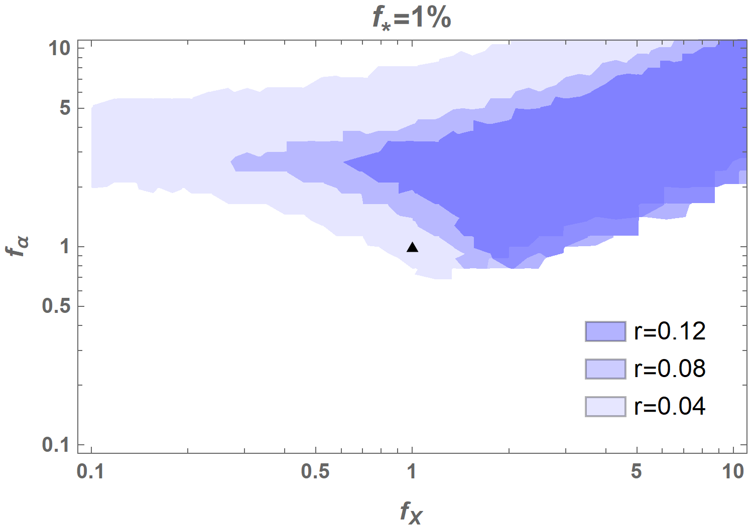
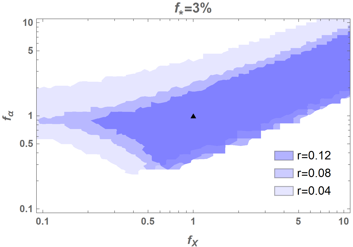
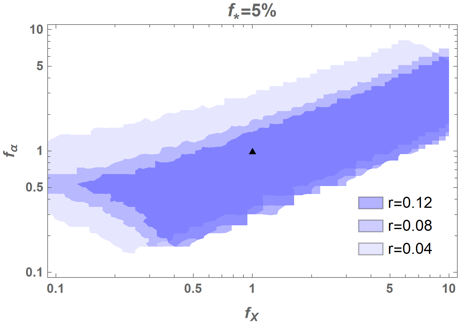
Figure 4: viable region in $f_{\alpha}$-$f_{X}$ space that can account for the anomalous EDGES absorption signal, with $r$ fixed to the benchmark values adopted in Fig. 3. The star formation efficiency is set to $1\%$, $3\%$ and $5\%$ from left to right. The black dot denotes the fiducial case $f_{\alpha}=f_{X}=1$.

References

Haslam et al. (1981)
C. Haslam,
U. Klein,
C. Salter,
H. Stoffel,
W. Wilson,
M. Cleary,
D. Cooke, and
P. Thomasson,
Astronomy and Astrophysics, vol. 100, no. 2, July 1981, p.
209-219. 100, 209
(1981).
Reich and Reich (1986)
P. Reich and
W. Reich,
Astronomy and Astrophysics Supplement Series (ISSN
0365-0138), vol. 63, no. 2, Feb. 1986, p. 205-288.
63, 205 (1986).
Roger et al. (1999)
R. S. Roger,
C. H. Costain,
T. L. Landecker,
and C. M.
Swerdlyk, Astron. Astrophys. Suppl. Ser.
137, 7 (1999),
eprint astro-ph/9902213.
Maeda et al. (1999)
K. Maeda,
H. Alvarez,
J. Aparici,
J. May, and
P. Reich,
Astronomy and Astrophysics Supplement Series
140, 145 (1999).
Fixsen et al. (2011)
D. J. Fixsen
et al., Astrophys. J.
734, 5 (2011),
eprint 0901.0555.
Fornengo et al. (2011)
N. Fornengo,
R. Lineros,
M. Regis, and
M. Taoso,
Phys. Rev. Lett. 107,
271302 (2011), eprint 1108.0569.
Caputo et al. (2023)
A. Caputo,
H. Liu,
S. Mishra-Sharma,
M. Pospelov, and
J. T. Ruderman,
Phys. Rev. D 107,
123033 (2023), eprint 2206.07713.
Cyr et al. (2024)
B. Cyr,
J. Chluba, and
S. K. Acharya,
Phys. Rev. D 109,
L121301 (2024), eprint 2308.03512.
Mittal and Kulkarni (2022)
S. Mittal and
G. Kulkarni,
Mon. Not. Roy. Astron. Soc.
510, 4992 (2022),
eprint 2110.11975.
Singal et al. (2018)
J. Singal et al.,
Publ. Astron. Soc. Pac. 130,
036001 (2018), eprint 1711.09979.
Singal et al. (2023)
J. Singal et al.,
Publ. Astron. Soc. Pac. 135,
036001 (2023), eprint 2211.16547.
Bowman et al. (2018)
J. D. Bowman,
A. E. E. Rogers,
R. A. Monsalve,
T. J. Mozdzen,
and N. Mahesh,
Nature 555, 67
(2018), eprint 1810.05912.
Barkana (2018)
R. Barkana,
Nature 555, 71
(2018), eprint 1803.06698.
Berlin et al. (2018)
A. Berlin,
D. Hooper,
G. Krnjaic, and
S. D. McDermott,
Phys. Rev. Lett. 121,
011102 (2018), eprint 1803.02804.
Muñoz and Loeb (2018)
J. B. Muñoz and
A. Loeb,
Nature 557,
684 (2018), eprint 1802.10094.
Pospelov et al. (2018)
M. Pospelov,
J. Pradler,
J. T. Ruderman,
and A. Urbano,
Phys. Rev. Lett. 121,
031103 (2018), eprint 1803.07048.
Brandenberger et al. (2019)
R. Brandenberger,
B. Cyr, and
R. Shi,
JCAP 09, 009
(2019), eprint 1902.08282.
Moroi et al. (2018)
T. Moroi,
K. Nakayama, and
Y. Tang,
Phys. Lett. B 783,
301 (2018), eprint 1804.10378.
Choi et al. (2020)
K. Choi,
H. Seong, and
S. Yun,
Phys. Rev. D 102,
075024 (2020), eprint 1911.00532.
Feng and Holder (2018)
C. Feng and
G. Holder,
Astrophys. J. Lett. 858,
L17 (2018), eprint 1802.07432.
Mittal et al. (2022)
S. Mittal,
A. Ray,
G. Kulkarni, and
B. Dasgupta,
JCAP 03, 030
(2022), eprint 2107.02190.
Fialkov and Barkana (2019)
A. Fialkov and
R. Barkana,
Mon. Not. Roy. Astron. Soc.
486, 1763 (2019),
eprint 1902.02438.
Caputo et al. (2021)
A. Caputo,
H. Liu,
S. Mishra-Sharma,
M. Pospelov,
J. T. Ruderman,
and A. Urbano,
Phys. Rev. Lett. 127,
011102 (2021), eprint 2009.03899.
Acharya et al. (2023)
S. K. Acharya,
B. Cyr, and
J. Chluba,
Mon. Not. Roy. Astron. Soc.
523, 1908 (2023),
eprint 2303.17311.
Chianese et al. (2019)
M. Chianese,
P. Di Bari,
K. Farrag, and
R. Samanta,
Phys. Lett. B 790,
64 (2019), eprint 1805.11717.
Dev et al. (2024)
P. S. B. Dev,
P. Di Bari,
I. Martínez-Soler,
and R. Roshan,
JCAP 04, 046
(2024), eprint 2312.03082.
Mirizzi et al. (2007)
A. Mirizzi,
G. G. Raffelt,
and P. D.
Serpico, Phys. Rev. D
76, 023001
(2007), eprint 0704.3044.
Ejlli (2018)
D. Ejlli, Eur.
Phys. J. C 78, 63
(2018), eprint 1609.06623.
Durrer and Neronov (2013)
R. Durrer and
A. Neronov,
Astron. Astrophys. Rev. 21,
62 (2013), eprint 1303.7121.
Addazi et al. (2024)
A. Addazi,
S. Capozziello,
and Q. Gan
(2024), eprint 2401.15965.
Ade et al. (2016)
P. A. R. Ade
et al. (Planck),
Astron. Astrophys. 594,
A19 (2016), eprint 1502.01594.
Reynés et al. (2021)
J. S. Reynés,
J. H. Matthews,
C. S. Reynolds,
H. R. Russell,
R. N. Smith, and
M. C. D. Marsh,
Mon. Not. Roy. Astron. Soc.
510, 1264 (2021),
eprint 2109.03261.
Obata et al. (2018)
I. Obata,
T. Fujita, and
Y. Michimura,
Phys. Rev. Lett. 121,
161301 (2018), eprint 1805.11753.
Bourhill et al. (2023)
J. F. Bourhill,
E. C. I. Paterson,
M. Goryachev,
and M. E. Tobar,
Phys. Rev. D 108,
052014 (2023), eprint 2208.01640.
Brandenburg et al. (2018)
A. Brandenburg,
R. Durrer,
T. Kahniashvili,
S. Mandal, and
W. W. Yin,
JCAP 08, 034
(2018), eprint 1804.01177.
Kolmogorov (1991)
A. N. Kolmogorov,
Proceedings of the Royal Society of London. Series A:
Mathematical and Physical Sciences 434,
9 (1991).
Kahniashvili et al. (2010)
T. Kahniashvili,
A. G. Tevzadze,
S. K. Sethi,
K. Pandey, and
B. Ratra,
Physical Review D 82
(2010).
Fixsen and Mather (2002)
D. Fixsen and
J. Mather,
The Astrophysical Journal 581,
817 (2002).
Pritchard and Loeb (2012)
J. R. Pritchard
and A. Loeb,
Rept. Prog. Phys. 75,
086901 (2012), eprint 1109.6012.
Koopmans et al. (2021)
L. V. Koopmans,
R. Barkana,
M. Bentum,
G. Bernardi,
A.-J. Boonstra,
J. Bowman,
J. Burns,
X. Chen,
A. Datta,
H. Falcke,
et al., Experimental astronomy
51, 1641 (2021).
Marsh et al. (2022)
M. C. D. Marsh,
J. H. Matthews,
C. Reynolds, and
P. Carenza,
Phys. Rev. D 105,
016013 (2022), eprint 2107.08040.
Mirizzi et al. (2009)
A. Mirizzi,
J. Redondo, and
G. Sigl,
JCAP 08, 001
(2009), eprint 0905.4865.
Mondino et al. (2024)
C. Mondino,
D. Pîrvu,
J. Huang, and
M. C. Johnson
(2024), eprint 2405.08059.
Tashiro et al. (2013)
H. Tashiro,
J. Silk, and
D. J. E. Marsh,
Phys. Rev. D 88,
125024 (2013), eprint 1308.0314.
Chen and Suyama (2013)
P. Chen and
T. Suyama,
Phys. Rev. D 88,
123521 (2013), eprint 1309.0537.
Ejlli et al. (2019)
A. Ejlli,
D. Ejlli,
A. M. Cruise,
G. Pisano, and
H. Grote,
Eur. Phys. J. C 79,
1032 (2019), eprint 1908.00232.
Fujita et al. (2020)
T. Fujita,
K. Kamada, and
Y. Nakai,
Phys. Rev. D 102,
103501 (2020), eprint 2002.07548.
Domcke and Garcia-Cely (2021)
V. Domcke and
C. Garcia-Cely,
Phys. Rev. Lett. 126,
021104 (2021), eprint 2006.01161.
Caloni et al. (2022)
L. Caloni,
M. Gerbino,
M. Lattanzi, and
L. Visinelli,
JCAP 09, 021
(2022), eprint 2205.01637.
Arias et al. (2012)
P. Arias,
D. Cadamuro,
M. Goodsell,
J. Jaeckel,
J. Redondo, and
A. Ringwald,
JCAP 06, 013
(2012), eprint 1201.5902.
Pritchard and Loeb (2008)
J. R. Pritchard
and A. Loeb,
Phys. Rev. D 78,
103511 (2008), eprint 0802.2102.