Proca stars in excited states

Abstract

In this paper we consider families of solutions for excited states of Proca stars in spherical symmetry. We focus on the first two excited configurations and perform a series of fully non-linear dynamical simulations in order to study their properties and stability. Our analysis reveals that excited Proca stars are always unstable against even very small perturbations, and their dynamical evolution can lead to three different final states: collapse to a black hole, dissipation, or migration to a different configuration in the ground state. We find that migration to the ground state can only occur in a small region of the parameter space of solutions with negative binding energy.

I Introduction

Exotic stars are hypothetical self-gravitating compact objects composed of different types of exotic matter. One particular type of exotic compact object (ECO) are the bosonic solitons, which represent stationary solutions of the Einstein field equations minimally coupled to massive, scalar or vector, complex fields. The scalar case corresponds to the usual boson stars [1, 2], while the vector case corresponds to the so-called Proca stars [3]; these models are commonly referred to as bosonic stars. In addition to bosonic stars, there are also Dirac stars [4] composed of complex spinor fields, further expanding the array of potential ECOs proposed in the literature. For a comparative analysis and review of these types of objects see for example [5, 6].

ECOs are theorized to be detectable due to their gravitational interactions with surrounding matter. This detection has the potential to offer valuable insights into the nature of the dark sector of the Universe, in particular serving as a promising environment for identifying the nature of dark matter (DM). Indeed, bosonic fields are considered viable candidates for dark matter due to their ability to clump together and form compact objects. Depending on the value of the mass parameter of the bosonic field, these objects can be considered as massive compact objects in galactic halos (MACHO’s), or can even acquire galactic scales in the case of ultralight masses [7, 8, 9]. These objects can also exhibit characteristics that mimic black holes [10], serve as potential sources of dark matter, and manifest in a variety of other phenomena [11]. One extensively studied scenario involves investigating whether these bosonic fields could undergo accretion inside stars, leading to the formation of stable configurations with observable effects. For a more detailed discussion we direct the reader to [12].

In this work we shall focus on Proca stars, that is spherically-symmetric self-gravitating configurations of a complex massive vector field (the Proca field) in four spacetime dimensions, and carrying a conserved Noether charge Q associated with a global U(1) symmetry. The first such self-gravitating solutions composed of massive spin-1 particles were reported in [3]. Numerical dynamical evolutions of these configurations have been performed in [13, 14], studying their stability and the various different phenomena that occur under perturbations of the Proca field in the ground state. Additionally, Proca stars have been set up in different astrophysical scenarios, such as those with rotation [15], charge [16], or more generalized models [17]. The primary objective of this work is to shed new light on the properties Proca stars in excited states, and in particular their stability under perturbations.

This paper is organized as follows. In Section II we present the Einstein–Proca system. In Section III we derive the spherically symmetric field equations for the stationary configurations corresponding to Proca stars and also discuss the total mass, total bosonic charge, and binding energy of the system, as well as the boundary conditions and the numerical methods that we have used. Section IV presents our results for the families of stationary configurations in the first two excited states, as well as the resuts of their dynamical evolutions under perturbations. We conclude in Section V.

II The Einstein-Proca Model

II.1 Action and fields equations

The Proca field is a massive complex vector field described by the complex potential 1-form $X_{\mu}$, from which we can obtain the field strength 2-form as $W_{\mu\nu}:=\nabla_{\mu}X_{\nu}-\nabla_{\nu}X_{\mu}$, where here $\nabla_{\mu}$ is the usual covariant derivative. The Lagrangian for the Proca field can then be written as:

$$\mathcal{L}_{P}=-\frac{1}{8\pi}\left(W_{\mu\nu}\bar{W}^{\mu\nu}+2m^{2}X_{\mu}\bar{X}^{\mu}\right)\;,$$ (1)

where $\bar{X}$, $\bar{W}$ denote complex conjugates, and $m$ is the mass parameter of the Proca field.

We will consider a self-gravitating Proca field minimally coupled to gravity. The combined Einstein-Proca system is then described by the following action:

$$\mathcal{S}=\int\left(\frac{R}{16\pi}+\mathcal{L}_{P}\right)\sqrt{-g}\>d^{4}x\;,$$ (2)

where $g$ is the determinant of the spacetime metric and $R$ is the curvature scalar. We use units such that $G=c=\hbar=1$, and the signature of spacetime metric is taken to be $(-,+,+,+)$. Variation of the action (2) with respect to the metric tensor leads to the Einstein field equations:

$$G_{\mu\nu}:=R_{\mu\nu}-\frac{1}{2}g_{\mu\nu}R=8\pi T_{\mu\nu}\;,$$ (3)

with $G_{\mu\nu}$ the Einstein tensor for our curved spacetime and $T_{\mu\nu}$ is the stress-energy tensor associated with the Proca field, which be derived from the Lagrangian (1) and takes the form:

$$T_{\mu\nu}=\frac{1}{4\pi}\left[-W_{\lambda(\mu}\bar{W}_{\nu)}^{\lambda}-\frac{g_{\mu\nu}}{4}\>W_{\alpha\beta}\bar{W}^{\alpha\beta}+m^{2}\left(X_{(\mu}\bar{X}_{\nu)}-\frac{g_{\mu\nu}}{2}X_{\lambda}\bar{X}^{\lambda}\right)\right]\;.$$ (4)

On the other hand, variation of the action with respect to the Proca field variables yields the Proca field equations:

$$\nabla_{\mu}W^{\mu\nu}=m^{2}X^{\nu}\;.$$ (5)

Unlike the case of the real massless spin-1 electromagnetic field, massive spin-1 fields such as the complex Proca field do not exhibit the same gauge invariance. Specifically, in the case of the Proca field the Lorenz condition is no longer a simple gauge choice but becomes instead a dynamical requirement that can be derived directly from (5):

$$\nabla_{\mu}X^{\mu}=0\;.$$ (6)

It is easy to see that the Einstein–Proca action above is invariant under a global $U(1)$ transformation of the form $X_{\mu}\longrightarrow e^{i\alpha}X_{\mu}$, with $\alpha$ constant. Noether’s theorem then implies the existence of a conserved 4-current given by:

$$j^{\mu}:=\frac{i}{8\pi}\left[\bar{W}^{\mu\nu}X_{\nu}-W^{\mu\nu}\bar{X}_{\nu}\right]\;,$$ (7)

such that:

$$\nabla_{\mu}j^{\mu}=0.$$ (8)

II.2 The Proca equations in 3+1 formalism

We work within the framework of the 3+1 formalism of general relativity, where the spacetime ($\mathcal{M}$, $g_{\mu\nu}$) can be foliated by Cauchy hypersurfaces $\Sigma_{t}$ parametrized by a global time function $t$, resulting in the standard Arnowitt–Deser–Misner (ADM) equations (see for example [18]). Additionally, by introducing auxiliary variables, one can modify the ADM equations to construct another formalism that is better adapted to stable and long-term numerical simulations, known as the Baumgarte–Shapiro–Shibata–Nakamura (BSSN) formalism [19, 20]. In particular, this BSSN formalism is the one used in our time evolution code adapted to spherical symmetry [21].

The 3+1 split of the metric takes the following form:

$$ds^{2}=\left(-\alpha^{2}dt^{2}+\beta_{i}\beta^{i}\right)dt^{2}+2\beta_{i}dtdx^{i}+\gamma_{ij}dx^{i}dx^{j}\;,$$ (9)

where $\gamma_{ij}$ is the three dimensional metric defined within the spatial hypersurfaces, $\alpha$ is the lapse function, and $\beta^{i}$ the shift vector. The unit normal vector $n^{\mu}$ to the spatial hypersurfaces has components given by

$$n^{\mu}=\left(1/\alpha,-\beta^{i}/\alpha\right)\;,\qquad n_{\mu}=\left(-\alpha,0,0,0\right)\;.$$ (10)

This timelike unit vector is identified with the 4-velocity of the so-called Eulerian observers.

We can do a 3+1 decomposition of the Proca field by defining the scalar potential $\phi$ and the 3-dimensional vector potential $a_{\mu}$ as:

$$\phi:=-n^{\mu}X_{\mu}\;,\qquad a_{\mu}:=\gamma_{\mu}^{\nu}X_{\nu}\;,$$ (11)

where $\gamma_{\mu}^{\nu}=\delta_{\mu}^{\nu}+n_{\mu}n^{\nu}$ is the projector operator onto the spatial hypersurfaces. From these potentials we can reconstruct the Proca potential $X_{\mu}$ as:

$$X_{\mu}=a_{\mu}+n_{\mu}\phi\;,$$ (12)

Notice that for the vector potential $a^{\mu}$ we have $a^{0}=0$, so that from now on we will only consider the spatial components $a^{i}$, with $a_{i}:=\gamma_{ij}a^{j}$. We further define the “electric” and “magnetic” fields associated with the Proca field as:

$$\mathcal{E}_{\mu}:=n^{\nu}W_{\mu\nu}\;,\qquad\mathcal{B}_{\mu}:=n^{\nu}W^{*}_{\mu\nu}\;,$$ (13)

where $W^{*}_{\mu\nu}$ is the dual field tensor defined as:

$$W^{*}_{\mu\nu}:=-\frac{1}{2}\>e_{\alpha\beta\mu\nu}W^{\mu\nu}\;,$$ (14)

with $e^{\alpha\beta\mu\nu}$ the Levi–Civita tensor. In terms of the electric and magnetic fields, the Proca field tensor and its dual can now be expressed as:

$$W_{\mu\nu} =n_{\mu}{\cal E}_{\nu}-n_{\nu}{\cal E}_{\mu}+E_{\mu\nu\lambda}{\cal B}^{\lambda}\;,$$ (15)

$$W^{*}_{\mu\nu} =n_{\mu}{\cal B}_{\nu}-n_{\nu}{\cal B}_{\mu}-E_{\mu\nu\lambda}{\cal E}^{\lambda}\;.$$ (16)

Based on the previous definitions, and manipulating the Proca field equations (5) together with the Lorenz condition (6), we can obtain the following set of time evolution equations for the Proca potentials and fields:

$$\frac{d}{dt}\>\phi =\alpha\phi K-D_{i}(\alpha a^{i})\;,$$ (17)

$$\frac{d}{dt}\>a_{i} =-\alpha\mathcal{E}_{i}-\partial_{i}(\alpha\phi)\;,$$ (18)

$$\frac{d}{dt}\>\mathcal{E}^{i} =\alpha\left(K\mathcal{E}^{i}+m^{2}a^{i}\right)+\left[D\times(\alpha\mathcal{B})\right]^{i}\;,$$ (19)

$$\frac{d}{dt}\>\mathcal{B}^{i}\> =\alpha K\mathcal{B}^{i}-\left[D\times(\alpha\mathcal{E})\right]^{i}\;,$$ (20)

with $d/dt:=\partial_{t}-\pounds_{\vec{\beta}}$, and where $D_{i}$ is the three-dimensional covariant derivative compatible with the spatial metric $\gamma_{ij}$ and $K$ is the trace of the extrinsic curvature tensor $K_{ij}$. Notice that again we only consider the spatial components of the electric and magnetic fields.

Furthermore, we also obtain the Gauss (21) and magnetic (22) constraints:

$$D_{i}\mathcal{E}^{i}+m^{2}\phi=0\;,$$ (21)

$$D_{i}\mathcal{B}^{i}=0\;.$$ (22)

One can also express the 3+1 matter terms coming from the stress–energy tensor (4) in terms of the 3+1 quantities associated with the Proca field. For the energy density we find:

$$\rho:=n^{\mu}n^{\nu}T_{\mu\nu}=\frac{1}{8\pi}\left[{\cal E}^{2}+{\cal B}^{2}+m^{2}\left(\phi^{2}+a^{2}\right)\right]\;,$$ (23)

where:

$${\cal E}^{2}:={\cal E}_{\alpha}\bar{\cal E}^{\alpha}={\cal E}_{i}\bar{\cal E}^{i}\;,\quad{\cal B}^{2}:={\cal B}_{\alpha}\bar{\cal B}^{\alpha}={\cal B}_{i}\bar{\cal B}^{i}\;,\quad\phi^{2}:=\phi\bar{\phi}\;,\quad a^{2}:=a_{i}\bar{a}^{i}\;.$$ (24)

For the momentum density we have:

$$J^{i}:=-\gamma^{i\mu}n^{\nu}T_{\mu\nu}=\frac{1}{8\pi}\left[e^{i}{}_{jk}\bar{{\cal E}}^{j}{\cal B}^{k}+m^{2}a^{i}\bar{\phi}+{\rm c.c.}\right]\;,$$ (25)

where now $e^{ijk}$ is the three dimensional Levi–Civita tensor defined as $e^{ijk}:=n_{\alpha}e^{\alpha ijk}$, and where c.c. indicates the complex conjugate of the previous terms.

Finally, for the 3D stress tensor we have:

$$S_{ij}:=\gamma^{\mu}_{i}\gamma^{\nu}_{j}T_{\mu\nu} =\frac{1}{8\pi}\left\{\gamma_{ij}\left({\cal E}^{2}+{\cal B}^{2}\right)-\left({\cal B}_{i}\bar{\cal B}_{j}+{\cal E}_{i}\bar{\cal E}_{j}+{\rm c.c.}\right)\right.$$

$$+\left.m^{2}\left[\left(a_{i}\bar{a}_{j}+{\rm c.c.}\right)-\gamma_{ij}\left(a^{2}-\phi^{2}\right)\right]\right\}\;.$$ (26)

One can also find 3+1 expressions for the conserved Noether current. In particular, the particle density is given by:

$$\rho_{Q}:=-n_{\mu}j^{\mu}=\alpha j^{0}=\frac{i}{8\pi}\left[a_{k}\bar{\cal E}^{k}-{\rm c.c.}\right]\;,$$ (27)

while for the particle flux we find:

$$j^{i}_{Q}:=\gamma^{i}_{\mu}j^{\mu}=\frac{i}{8\pi}\left[\phi\bar{\cal E}^{i}+E^{ijk}a_{j}\bar{\cal B}_{k}-{\rm c.c.}\right]\;.$$ (28)

III Proca stars

To study stationary configurations corresponding to Proca stars we first assume spherical symmetry. The line element in spherical coordinates $(t,r,\theta,\phi)$ can then be written as:

$$ds^{2}=-\alpha^{2}dt^{2}+\psi^{4}\left(Adr^{2}+r^{2}Bd\Omega^{2}\right)\;,$$ (29)

with $\psi$ a conformal factor, and where $d\Omega^{2}=d\theta^{2}+\sin^{2}\theta d\phi^{2}$ is the standard solid angle element. In general the metric functions $(\alpha,\psi,A,B)$ are functions of both time $t$ and radius $r$, though for the case of stationary configurations they will depend only on $r$. Notice that in principle we don’t need to introduce the conformal factor $\psi$, and indeed we will take it to be equal to 1 for our stationary configurations, but we do need it for the BSSN formalism used in the dynamical simulations that we will consider later. In the context of this work, the assumption that the shift vector vanishes, $\beta^{i}=0$, is adequate for our time evolutions. In order to obtain our stationary configurations we will further restrict ourselves to using the areal radial coordinate, so in this Section we will take $B=\psi=1$.

Proca stars (PSs) are self-gravitating solutions in spherical symmetry for which the Proca field exhibits a harmonic time dependence of the form of $e^{-i\omega t}$, resulting in a time-independent stress-energy tensor which leads to a static spacetime metric. Notice that in spherical symmetry the magnetic field vanishes, while the vector potential and the electric field only have a non-zero radial component. We then propose the following ansatz for the scalar potential and the radial components of the vector potential and the electric field:

$$\begin{split}\phi(r,t)&=\varphi(r)e^{-i\omega t}\;,\\ a_{r}(r,t)&=\textit{i}a(r)e^{-i\omega t}\;,\\ \mathcal{E}^{r}(r,t)&=e(r)e^{-i\omega t}\;,\end{split}$$ (30)

with $\omega$ a real constant corresponding to the oscillation frequency of the Proca field, and where the functions $\varphi(r)$, $a(r)$ and $e(r)$ are real and depend only on the radial coordinate $r$. The explicit factor of $i$ introduced in the ansatz for the radial component of the vector potential $a_{r}$ is there in order to guarantee that both the momentum density (25) and the particle flux coming from the conserved Noether current (28) vanish, as they should for a static solution. In our case the momentum density reduces to:

$$J_{r}=\frac{m^{2}}{8\pi}\left[a_{r}\bar{\phi}+c.c\right]=\frac{m^{2}}{8\pi}\left[ia\varphi+c.c\right]=0\;,$$ (31)

while the particle flux reduces to:

$$j^{r}_{Q}=\frac{i}{8\pi}\left[\phi\bar{\mathcal{E}}^{r}-c.c.\right]=\frac{i}{8\pi}\left[\varphi e-c.c.\right]=0\;.$$ (32)

By substituting our harmonic anzats (30) into the evolution equations (17)—(19) and the Gauss constraint (21), we can derive a set of ordinary differential equations in $r$ to solve for our Proca star configurations. In order to simplify some expressions we work with $F(r):=\alpha\varphi$ instead of $\varphi$ itself. Once the system is solved, $\varphi$ can be immediatly reconstructed as $\varphi=F/\alpha$.

From the evolution equation for $a_{r}$, equation (18), we find:

$$\partial_{r}F=-\omega a-\alpha eA\;.$$ (33)

On the other hand, from the evolution equation for $\mathcal{E}^{r}$, equation (19), we can solve explicitly for $e$ to find:

$$e=-\frac{\alpha m^{2}a}{\omega A}\;,$$ (34)

so that our equation for $F$ then becomes:

$$\partial_{r}F=\omega a\left(\frac{\alpha^{2}m^{2}}{\omega^{2}}-1\right)\;.$$ (35)

We can also obtain a differential equation for $a$ from the evolution equation for $\phi$, equation (17). We find:

$$\partial_{r}a=\frac{\omega\varphi A}{\alpha}-a\left(\frac{2}{r}-\frac{\partial_{r}A}{2A}+\frac{\partial_{r}\alpha}{\alpha}\right)\;.$$ (36)

Finally, from the Gauss constraint we find:

$$\partial_{r}e=-e\left(\frac{2}{r}+\frac{\partial_{r}A}{2A}\right)-m^{2}\varphi\;.$$ (37)

Notice that this last equation in principle is not necessary, as we already have an explicit expression for $e$ in equation (34) above. Indeed, one can show that this last equation is completely consistent with that solution. However, equation (37) will be necessary when we consider perturbed Proca stars below.

We still need equations for the lapse function $\alpha$ and the radial metric $A$. For the radial metric we use the Hamiltonian constraint, which in spherical symmetry and with our coordinate choices reduces to:

$$\partial_{r}A=A\left[\frac{(1-A)}{r}+8\pi rA\rho\right]\;,$$ (38)

with $\rho$ the energy density. The equation for the lapse comes from our choice of using the areal radius, which in turn implies that the angular component of the extrinsic curvature has to vanish for all time, which through the ADM equations leads to the so-called “polar-areal” gauge condition that takes the form:

$$\partial_{r}\alpha=\alpha\left[\frac{\left(A-1\right)}{2r}+4\pi rAS^{r}_{r}\right]\;.$$ (39)

Notice that the equations for $\alpha$ and $A$ above have matter terms on the right hand side corresponding to the energy density $\rho$ and the component $S^{r}_{r}$ of the stress tensor. Using now equations (23) and (26) one can show that in our case those quantities reduce to:

$$\rho =+\frac{1}{8\pi}\left[Ae^{2}+m^{2}\left(\varphi^{2}+a^{2}/A\right)\right]\;.$$ (40)

$$S^{r}_{r} =-\frac{1}{8\pi}\left[Ae^{2}-m^{2}\left(\varphi^{2}+a^{2}/A\right)\right]\;.$$ (41)

As a final comment, equation (36) above has terms on the right hand side that involve derivatives of $\alpha$ and $A$. But we can substitute those derivatives using the equations for $\alpha$ and $A$ that we just found, so that the equation for $a$ now becomes:

$$\partial_{r}a=\frac{A\omega F}{\alpha^{2}}-a\left[\frac{1}{r}\left(1+A\right)+4\pi rA\left(S^{r}_{r}-2\rho\right)\right]\;.$$ (42)

The final system of equations that we need to solve for ($A,\alpha,F,a$) is then (38), (39), (35) and (42), with $e$ given by (34).

III.1 Boundary conditions

We need to solve the system of first order differential equations (38), (39), (35), (42) for the functions $(A,\alpha,F,a)$ in order to obtain the family of Proca stars, subject to a series of physical boundary conditions. The boundary conditions for the radial metric come from demanding regularity at the origin:

$$A(r=0)=1\;,\qquad\left.\partial_{r}A\right|_{r=0}=0\;.$$ (43)

Notice that we must ask for $A(r=0)=1$ in order for the metric to be locally flat there. Also, we must have $\lim_{r\rightarrow\infty}A=1$ in order to have an asymptotically flat spacetime, though the structure of equation (38) guarantees that this is the case if the energy density decays fast enough. For the lapse we ask for regularity at the origin, and also to recover Minkowski spacetime far away, which corresponds to:

$$\lim_{r\rightarrow\infty}\alpha=1\;,\qquad\left.\partial_{r}\alpha\right|_{r=0}=0\;.$$ (44)

For the scalar potential $\varphi$ (or equivalently $F$) we ask again regularity at the origin, and $\varphi$ going to zero at infinity:

$$\lim_{r\rightarrow\infty}\varphi=0\;,\qquad\left.\partial_{r}\varphi\right|_{r=0}=0\;.$$ (45)

Finally, the vector potential $a$ must also go to zero at infinity, and since it is the radial component of a vector it must vanish at the origin as well:

$$a(r=0)=0\;,\qquad\lim_{r\rightarrow\infty}a=0\;.$$ (46)

We can in fact be somewhat more precise. For an asymptotically flat spacetime, for large $r$ the equations for $\varphi$ and $a$ become (taking $A=1$ and $\rho=S^{r}_{r}\simeq 0$):

$$\partial_{r}\varphi=\frac{\omega a}{\alpha_{\infty}}\left(\frac{\alpha^{2}_{\infty}m^{2}}{\omega^{2}}-1\right)\;,\qquad\partial_{r}a=\frac{\omega\varphi}{\alpha_{\infty}}\;,$$ (47)

with $\alpha_{\infty}$ the asymptotic value of the lapse (which as we already mentioned should be equal to 1, but see below). Combining both equations we find:

$$\partial^{2}_{r}\varphi=\left(m^{2}-\frac{\omega^{2}}{\alpha^{2}_{\infty}}\right)\varphi\;,$$ (48)

which can be easily solved to find:

$$\varphi=e^{\pm(m^{2}-\omega^{2}/\alpha^{2}_{\infty})^{1/2}r}\;.$$ (49)

From this we see that in order for $\varphi$ to be real we must necessarily have $\omega^{2}<\alpha^{2}_{\infty}m^{2}$. But notice that in that case we can have both increasing and decreasing exponential solutions. The increasing solutions are unphysical, as they are not compatible with an asymptotically flat spacetime. In fact, one finds that we only have exponentially decaying solutions for a discrete set of values of the frequency $\omega$, which implies that we need to solve an eigenvalue problem.

We can also give some more detail for the boundary conditions at the origin. The equation for $\partial_{r}a$ has a term that goes as $a/r$. This implies that for regularity close to the origin we must have $a\sim k_{a}r$, with $k_{a}$ some constant. Substituting this in the equation we find:

$$k_{a}=\frac{\omega\varphi_{0}}{3\alpha_{0}}\;,$$ (50)

with $\alpha_{0}=\alpha(r=0)$ and $\varphi_{0}=\varphi(r=0)$. In the same way we see that in the equation for $\partial_{r}A$ there is a term that goes as $(1-A)/r$. This means that close to the origin we must have $A\sim 1+k_{A}r^{2}$. Substituting this in the equation we now find:

$$k_{A}=\frac{8\pi}{3}\>\rho_{0}\;,$$ (51)

with $\rho_{0}=\rho(r=0)$. These conditions turn out to be very useful in order to start the numerical integration of our equations from the origin.

Numerically, we solve our system of equations starting from the origin, where we choose as our free parameter the value of $\varphi_{0}$ and a trial value for the frequency $\omega$. We then integrate the system outwards (using a fourth order Runge–Kutta method), and keep modifying the value of $\omega$ with a shooting algorithm until we find a solution that decays far away.

There is one last detail that must be considered. Since initially we don’t know the value of the lapse $\alpha$ at the origin we start by taking $\alpha_{0}=1$. However, what we really want is $\alpha$ to become zero at infinity. But this is not a serious problem since the equation for $\partial_{r}\alpha$ is linear in $\alpha$, so we can always rescale the solution at the end using the asymptotic value of the lapse $\alpha_{\infty}$ (obtained by extrapolation assuming that the lapse far away behaves as $\alpha\simeq\alpha_{\infty}-c/r$ for some positive constant $c$). However, in order for this to still be a solution of the whole system we must also rescale the frequency $\omega$ by the same factor. In particular this implies that our initial trial frequency is in general such that $\omega>m$, but once we rescale it we will have $\omega<m$. Notice also that if we solve the system for $F$ instead of $\varphi$, then we also need to rescale $F$ by the same factor in order to maintain $\varphi=F/\alpha$ the same as before.

III.2 Total mass and particle number

When working in terms of the areal radius, the total mass $M$ of the spacetime can be shown to be the integral of the energy density over a flat volume element (this can be shown directly from the Hamiltonian constraint for a static spacetime when using the areal radius):

$$M=4\pi\int_{0}^{\infty}\rho r^{2}dr\;,$$ (52)

with the energy density of matter $\rho$ given by equation (40).

Similarly, the existence of a Noether current implies a conserved charge $Q$ given by:

$$Q:=\int\rho_{Q}\gamma^{1/2}d^{3}x=4\pi\int_{0}^{\infty}\rho_{Q}A^{1/2}r^{2}dr\;,$$ (53)

with $\rho_{Q}$ the particle density given by (27), and where we used the fact that the determinant of the spatial metric is given by $\gamma=Ar^{2}\sin^{2}\theta$ (notice that for this integral we do need to use the physical curved volume element). In our case the particle density $\rho_{Q}$ reduces to:

$$\rho_{Q}=-\frac{ae}{4\pi}=\frac{\alpha m^{2}a^{2}}{\omega A}\;.$$ (54)

The integrated charge $Q$ represents the total number of bosonic particles, so that the product $mQ$ corresponds to the total rest mass of the system. On the other hand, the total mass $M$ includes contributions from kinetic and potential energies, as well as the rest mass. Therefore, we can define a binding energy as:

$$U:=M-mQ\;,$$ (55)

in order to isolate the kinetic and potential contributions. This means that those solutions with $mQ>M$ will have a negative binding energy, $U<0$, and will correspond to gravitationally bound stars. Conversely, solutions with $mQ<M$ have positive binding energy $U>0$, making them gravitationally unbound (and hence should be expected to be unstable against perturbations).

We can also use the mass integral above to define an effective radius $R_{99}$ which contains 99% of the total mass. This effective radius is necessary due to the fact that, as we mentioned above, for Proca stars the energy density decays exponentially far away implying that there is no real surface.

III.3 Perturbations

In previous sections we derived the equations that we need to solve in order to obtain stationary Proca star configurations, we will show families of such solutions for the ground state and the first two excited states in Section IV.1 below. However, one of the aims of this paper is to study the dynamical stability of perturbed Proca star configurations. We will therefore also consider self-consistent perturbations to the stationary Proca star solutions.

Once we have a stationary solution we will construct a perturbation to it in the following way:

1. We add a small perturbation to the scalar potential $\varphi(r)$ (in practice we add it to $F(r)$), typically a gaussian, leaving the vector potential $a(r)$ unchanged. The perturbation in $\varphi$ (or $F$) must be even with respect to reflections on the origin in order to maintain regularity there. For example, if the add a gaussian centered on a point $r=r_{0}$ away from the origin, we must also add a similar gaussian centered on $r=-r_{0}$ in order to guarantee that we still have $\partial_{r}\varphi(r=0)=0$. Notice also that if we only modify the real part of the scalar potential while leaving the vector potential purely imaginary, the momentum density $J_{r}$ remains zero. Similarly, since the scalar potential remains real the electric field $\mathcal{E}^{r}$ will also be purely real, so that the particle flux $j^{r}_{Q}$ also remains zero.

2. We solve again the Hamiltonian constraint (38), the polar slicing condition (39), and the Gauss constraint (37) for the functions $(A,\alpha,e)$. Notice that we now can not use the explicit solution for the electric field $e(r)$ given by (34) since it is no longer valid for a perturbed star, so we must solve for $e(r)$ using equation (37).

The procedure just described results in consistent initial data for a perturbed Proca star. Of course, our perturbed star will no longer be stationary. However, as mentioned above, the momentum density and particle flux are initially zero, which is consistent with taking an initially vanishing extrinsic curvature. Our perturbed initial data will then result in a momentarily static geometry corresponding to a moment of time symmetry.

Once we have the perturbed initial data we evolve it in time using the OllinSphere code already described in [22, 23, 24, 25, 26], which implements a BSSN formulation adapted to spherical symmetry [21]. For the evolution of the Proca field variables we use equations (17)-(19), which in our case reduce to:

$$\partial_{t}\phi =\alpha K\phi-\frac{1}{A\psi^{4}}\>\partial_{r}\left(\alpha a_{r}\right)+\frac{\alpha a_{r}}{A\psi^{4}}\left(\frac{\partial_{r}A}{2A}-\frac{\partial_{r}B}{B}-2\>\frac{\partial_{r}\psi}{\psi}-\frac{2}{r}\right)\;,$$ (56)

$$\partial_{t}a_{r} =-\alpha A\psi^{4}\mathcal{E}^{r}-\partial_{r}\left(\alpha\phi\right)\;,$$ (57)

$$\partial_{t}\mathcal{E}^{r} =\alpha\left(K\mathcal{E}^{r}+\frac{m^{2}a^{r}}{A\psi^{4}}\right)\;.$$ (58)

Notice that even if for our initial data we took the conformal factor $\psi$ and the angular metric component $B$ equal to 1 in the metric (29), this will not remain true for a dynamical simulation. One must also remember that all three quantities $(\phi,a_{r},\mathcal{E}^{r})$ are complex, so we must evolve their real and imaginary parts separately.

IV Results

IV.1 Families of stationary solutions for ground and excited states

The set of ordinary differential equations is integrated numerically using a fourth-order Runge-Kutta method. The code takes a central value of the potential scalar $\varphi_{0}$ as an input parameter, and then employs a shooting algorithm to determine the value of the frequency $\omega$ that corresponds to the asymptotically decaying solution of the scalar potential. For simplicity, we set the value of the Proca mass parameter to $m=1$, but notice that the solutions can later be rescaled to arbitrary values of $m$ since our system of equations is invariant under the rescaling:

$$m\rightarrow\lambda m\;,\qquad\omega\rightarrow\lambda\omega\;,\qquad r\rightarrow r/\lambda\;,\qquad e\rightarrow\lambda e\;.$$ (59)

In this section we will present the properties of the stationary configurations for three families of Proca star solutions, corresponding to the ground state and the first two excited states. Table 1 shows the parameters that correspond to the maximum mass configuration for all three families of solutions. In particular we show the central value of the scalar potential $\varphi_{0}$, the corresponding frequency $\omega$, the total mass $M$, the binding energy $U$, as well as the effective radius $R_{99}$ and effective compactness defined as $C_{99}:=M/R_{99}$. Our data can be compared with that already reported in [27, 14, 28] for the ground state. However, we also explore the properties of the first two excited states, which correspond to solutions with one or two nodes in the vector potential $a(r)$ (notice the scalar potential $\varphi(r)$ already has one node even in the ground state, see below).

State	$\varphi_{0}$	$\omega$	$M_{max}$	$U$	$C_{99}$	$R_{99}$
ground	0.1410	0.8698	1.058	-0.030	0.0900	11.75
1° excited	0.1636	0.8828	1.797	-0.047	0.0898	20.01
2° excited	0.1805	0.8880	2.526	-0.064	0.0899	28.07

Table 1: We show the parameters that characterize the maximum mass configurations for Proca stars in the ground state and the first two excited states.

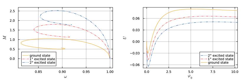
Figure 1: Left panel: Total integrated mass $M$ (in units of $M^{2}_{Planck}/m$) as a function of frequency $\omega$. We observe that as the excitation level of the star increases the total mass $M$ also increases. Right panel: Binding energy $U$ as function of $\varphi_{0}$. For each of the families $U$ has a global minimum, which corresponds to the solutions with maximum mass of Table 1.

We show our three different families of solutions in Figure 1. The left panel shows the total integrated mass $M$ as a function of the oscillation frequency $\omega$, while the right panel shows the binding energy $U$ as a function of the central value of the scalar potential $\varphi_{0}$. We can observe that excited states have in general higher masses. Additionally, we also find that the frequency domain is bounded for all three families, showing the characteristic spiral pattern in the mass versus frequency plot that also appears for boson stars, with the minimum frequency increasing with the excitation level. Also, for all three families there is a value of the central field for which the binding energy reaches a minimum, which in fact corresponds to the solutions with maximum mass. As we increase the value of $\varphi_{0}$ further the binding energy also increases and eventually becomes positive, corresponding to solutions that are no longer gravitationally bound.

Solutions with negative binding energy in all three families can be further separated into solutions to the left and to the right of the minimum binding energy $U$ (maximum mass $M$) in the right panel of Figure 1. Naively, one could expect that all solutions with negative binding energy should be stable under perturbations since they represent gravitationally bound stars. However, as has already been shown [14], this is not true even for solutions in the ground state: configurations to the right of the minimum are unstable to perturbations and can either collapse to a black hole or migrate to a configuration on the stable left branch (this is the same in the case of boson stars). Having a solution with $U<0$ is therefore a necessary but not sufficient condition for the stability of the Proca stars in the ground state. The purpose of this paper is to investigate if something similar happens for solutions in excited states. We will return to this point when we consider dynamical simulations below.

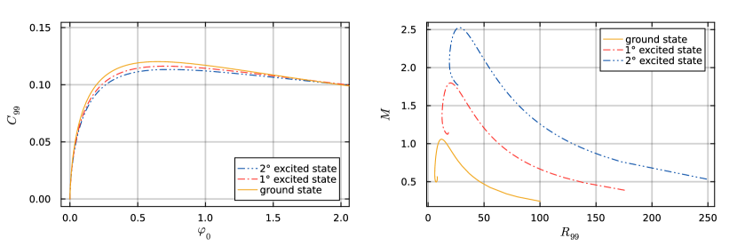
Figure 2: Left panel.: The effective compactness defined as $C_{99}=M/R_{99}$ versus $\varphi_{0}$. Right panel: Total mass $M$ as a function of the effective radius $R_{99}$. We observe that excited Proca stars increase in both mass and radius.

In Figure 2 we consider the effective radius and compactness of our three families of solutions. The right panel shows the total mass $M$ as a function of the effective radius $R_{99}$, while the left panel shows the effective compactness defined as $C_{99}=M/R_{99}$ as a function of $\varphi_{0}$. Notice that despite the fact that Proca stars in the ground state have in general a lower mass than those in excited states, they exhibit greater compactness. This is not too surprising since Proca stars in excited states are generally larger in size, as can be seen in the right panel of the Figure. For the ground state family the effective compactness reaches a maximum value of $C_{99}\simeq 0.12$. This value is still far from $C=0.5$ corresponding to the compactness for a Schwarzschild black hole, but is comparable with other kind of compact objects [29].

In order to better illustrate the properties of our solutions we consider three particular configurations in Figure 3. We consider three solutions with the same central value of the scalar potential $\varphi_{0}=0.081$: One in the ground state, one in the first excited state, and one in the second excited state. All three configurations can be shown to have negative binding energy. Panel (a) shows the density profile $\rho(r)$ for all three solutions. We notice that the ground state possesses a single core of matter, while the excited states have a core and shells surrounding it, and as a result the effective radii of the excited configurations are larger. The first excited state has one such shell outside the core, while the second excited state has two shells (compare this with the analogue case for excited boson stars in [30]).

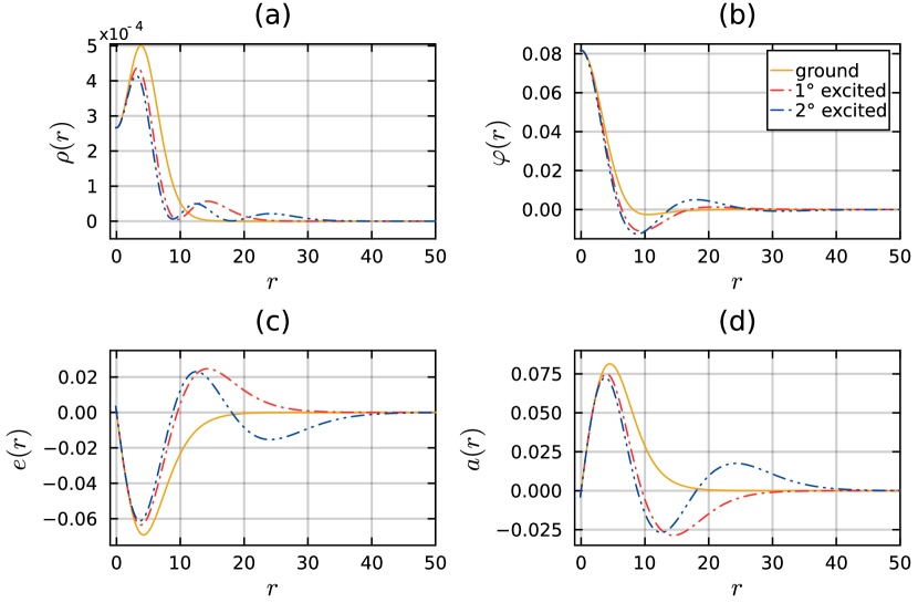
Figure 3: We show the solutions for the ground state and the first two excited states for the same central value of the scalar potential $\varphi_{0}=0.081$ (the color scheme is the same for all four figures). Panel (a) shows energy density $\rho(r)$. Panels (b) , (c), and (d) show the profiles for the scalar potential $\varphi(r)$, the electric field $e(r)$, and radial component of vector potential $a(r)$.

The other three panels of the figure show the profile functions $\varphi(r)$, $e(r)$ and $a(r)$ for the ground and first two excited states. All these functions decay rapidly far away, as expected. We can also observe that the number of nodes increases with the excitation levels. The scalar function $\varphi(r)$ in the ground state already has one node, followed by the first and second excited states with two and three nodes, respectively. Additionally, in the ground state both the vector potential $a(r)$ and the Proca electric field $e(r)$ have no nodes, while they have one node in the first excited state and two nodes in the second.

IV.2 Dynamical evolutions and stability

The values presented in Table 1 will serve as a reference for choosing models for our dynamical evolutions of perturbed Proca star configurations. In all the numerical simulations presented below we always add a small Gaussian perturbation centered at the origin and with unit width to the scalar potential $\varphi(r)$, while leaving the vector potential $a(r)$ unchanged. The amplitude of this perturbation is always taken as 5% of the maximum amplitude of the scalar potential of the original stationary solution. As mentioned above, once we add the perturbation to $\varphi(r)$ we solve again the the Hamiltonian and Gauss constraints to obtain self-consistent initial data.

IV.2.1 First excited state

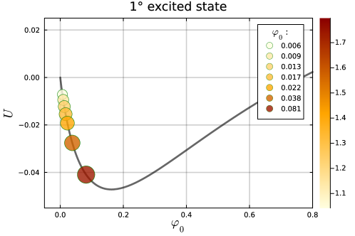
Figure 4: Binding energy $U$ as function of $\varphi_{0}$ for the first excited state. The circles show the 7 models that we considered for our perturbed dynamical evolutions. The color bar indicates the scale of the total integrated mass $M$ of the unperturbed stationary configurations. The size of each circle in the plot is proportional to the total mass, and increases as we approach the the minimum of the binding energy.

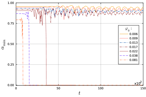
Figure 5: Evolution of the central value of the lapse function $\alpha$ for the first excited state for all 7 models studied. For the 4 models with lower values of $\varphi_{0}$ migration is observed, while for models with higher values of $\varphi_{0}$ the central lapse collapses to zero indicating the formation of a black hole.

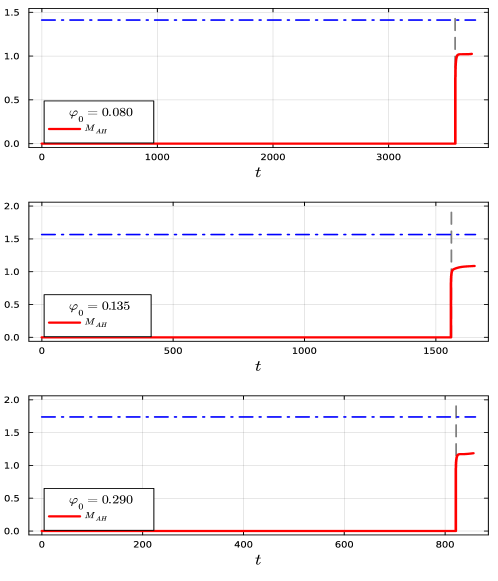
Figure 6: Apparent horizon mass a a function of time time for the three models in the first excited state that exhibit collapse to a black hole. The time at which the code first finds an apparent horizon corresponds to the dashed vertical line. The dash-dot horizontal line represents the value of the total integrated mass of the spacetime at $t=0$.

Figure 4 shows a plot of the binding energy $U$ for Proca stars in the first excited state as a function of the central value of the scalar potential $\varphi_{0}$. In the Figure we also indicate 7 different models that we considered for our dynamical evolutions of perturbed initial data. Notice that all these models have negative binding energy, and are to the left of the minimum in $U$ (corresponding to the maximum mass $M$), the region that one would expect to be more stable.

Figure 5 shows the value of the lapse function $\alpha$ at $r=0$ as a function of time for all 7 models during their evolution. The behavior of the lapse provides us with important information about the type of phenomena occurring during the evolution of our perturbed Proca stars. We observe two types of behavior corresponding to migration to a more stable solution, and collapse to a black hole. This does not imply that dispersion phenomena can not occur; in fact, we find that dispersion seems to predominate when the Proca stars have positive binding energy, but here we want to concentrate on the negative binding energy configurations.

The central lapse collapses to zero for the models with $\varphi_{0}=$ 0.081, 0.038, and 0.022, indicating the formation of a black hole. The behavior of the lapse is similar in all 3 models, the main difference being the time at which the collapse occurs. In particular, we find that if the star’s mass is closer to the maximum (binding energy closer to the minimum) it becomes more unstable, leading to a faster collapse. In order to confirm the formation of a black hole we look for apparent horizons during the evolution. Figure 6 shows the apparent horizon mass as a function of time. We can observe that the apparent horizon suddenly appears in all three cases (at different times), coinciding with the time at which the central lapse collapses to zero. The horizon mass is always smaller that the initial total mass of the spacetime (shown as a blue dashed line). We only show the horizon mass for a short time after its formation, as later the numerical errors become too large due to the well known phenomenon of slice stretching (we are evolving without a shift vector).

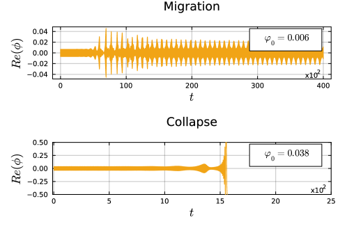
Figure 7: Evolution of the real part of the scalar potential $\phi$ at $r=0$ for the models with $\varphi_{0}=0.006$ (upper panel) and $\varphi_{0}=0.038$ (lower panel). These models illustrate the behavior of the field’s oscillations when the Proca star is either migrating to another more stable solution, or collapsing into black hole.

We will now focus on the migration phenomena which occurs for the models with $\varphi_{0}=$ 0.017, 0.013, 0.009 and 0.006. These models have lower masses and a binding energy closer to zero. In all these cases the central value of the lapse begins to oscillate irregularly after some time around a mean value that stays away from zero, and is also lower than its original value. However, this provides little information as to the final state of the Proca star. To gain a better understanding of what is happening, in Figure 7 we show the evolution of the oscillations of the real part of the scalar potential $\phi$ evaluated at $r=0$ for the model with $\varphi_{0}=0.006$, which migrates (upper panel), and the model with $\varphi_{0}=0.038$, which collapses to a black hole (lower panel). Notice that for the collapsing model the oscillations become very large and eventually stop due to the collapse of the lapse there, while for the migrating model the oscillations settle on a quite regular modulated pattern after some time. We observe a similar behavior for the other migrating models.

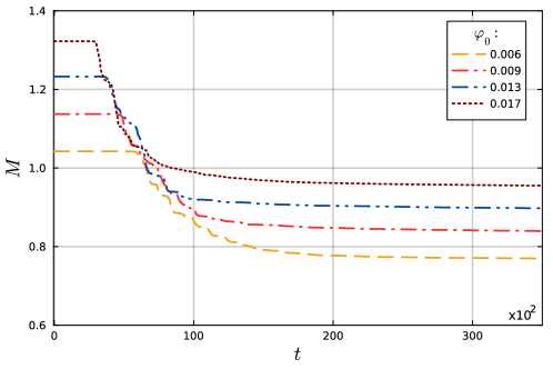
Figure 8: Evolution of the total mass $M$ at the outer boundary for models in the first excited state that exhibit migration.

For the migrating models it is important to determine the direction of this migration, or in other words the final asymptotic state. In order to do this we analyze the total integrated mass at the boundary of our numerical domain for the 4 migrating models; this is shown in Figure 8. The different configurations start with an initial total mass $M_{i}$ corresponding to that of the (slightly perturbed) stationary solution. However, due to the perturbation, a fraction of this mass — which in all 4 cases turns out to be approximately 25% — is lost during the evolution as the star ejects part of the Proca field to infinity. As a result, the total mass at the boundary decreases over time to some asymptotic value $M_{f}$. Notice also that the total mass remains initially constant for a while, which corresponds to the time it takes for the ejected field to reach the boundary of our computational domain.

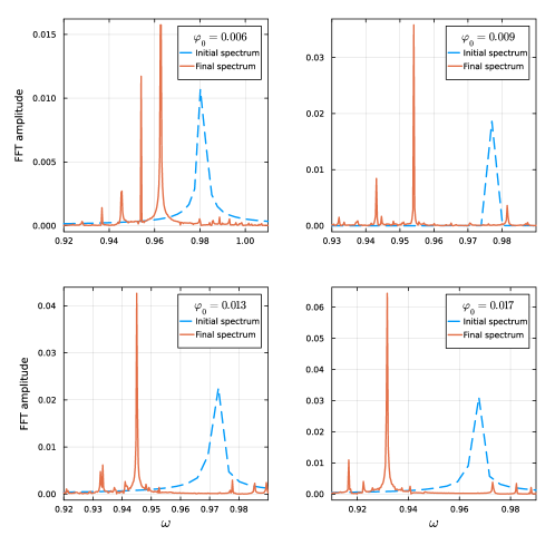
Figure 9: Fourier transform of the time evolution of the real part of $\phi$ for models in the first excited state, specifically for those models that exhibit the migration phenomena. The dashed blue lines correspond to the initial frequency spectrum, while the solid red lines represent the final spectrum. In the final stage, the migrating stars have more than one frequency present, but there is always one dominant frequency that stands out.

We can analyze the final state of our configurations further by doing a Fast Fourier Transform (FFT) of the real part of the scalar potential $\phi$ evaluated at $r=0$, both at the beginning and at the final stages of the time evolutions. This is shown in Figure 9. The dashed blue line shows the FFT for the initial stages of the evolution for all 4 migrating models. In each case we can see a single peak frequency $\omega_{i}$, which coincides with the oscillating frequency of our original stationary solution. The solid red lines correspond to the FFT for the late stages of our evolutions. The spectra for the different models have clearly changed in time, and now show a very different dominant frequency $\omega_{f}$, plus a few other lower amplitude modulating frequencies. To obtain the FFT’s, we divide the evolution into initial and final stages based on the behavior of the oscillation of the real part of the scalar potential at $r=0$. We select an appropriate time interval for each migrating case. Generally, the initial stage consists of only a short time interval because the oscillations of the perturbed solution increase rapidly. The final stage corresponds to a later time when the oscillations have settled into a regular modulated pattern. We only exclude a short portion of the evolution, which represents the transition phase in the middle of the evolutions.

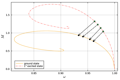
Figure 10: Using the data for the final dominant frequency $\omega_{f}$ and final mass and $M_{f}$ for our migrating models in the first excited state (see Table 2 of the Appendix), we can find the final configuration in the ground state family of solutions to which they are migrating.

By considering the final total mass $M_{f}$ and the final dominant frequency $\omega_{f}$, we can determine the direction of migration for the perturbed Proca stars in the first excited state. Upon comparing these final parameters with the families of stationary solutions, we conclude that the migration is towards configurations in the stable branch of the ground state, see Figure 10. All this data is summarized in Table 2 of the Appendix.

IV.2.2 Second excited state

As shown in Figure 11, for the case of the second excited states we have also selected models with negative binding energy to the left of the minimum, but in this case even closer to the origin. The reason for this is the general trend of instability for the Proca stars: for higher excited states collapse to a black hole becomes more likely, and it is harder to find models that migrate to a stable configurations.

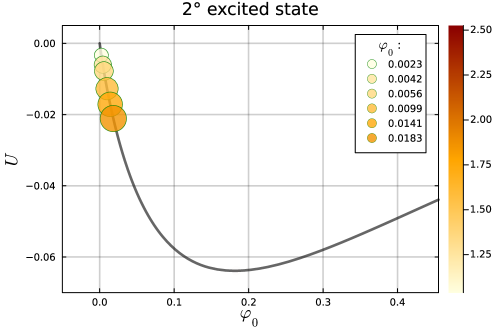
Figure 11: Binding energy $U$ as function of $\varphi_{0}$ for the second excited state. The circles show the 6 models that we considered for our perturbed dynamical evolutions. As before, the color bar and the size of the circles indicate the initial total mass.

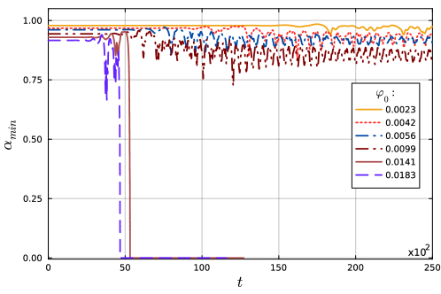
Figure 12: Evolution of the central value of the lapse function $\alpha$ for the second excited state for all the 6 models studied. For the models with lower values of $\varphi_{0}$ migration is observed, while the remaining 2 models collapse into black hole.

Figure 13: Apparent horizon mass as a function of time for the 2 collapsing models in the second excited state. The dashed vertical line indicates the time at which an apparent horizon is first found, and the dashed-dot horizontal line represents the value of the total integrated mass at $t=0$.

Figure 12 shows again the central value of the lapse function $\alpha$ as a function of time for these 6 models. Similar behaviors are observed, with migration appearing for the 4 lower mass models, and collapse to a black hole for the other 2. Figure 13 shows the apparent horizon mass as a function of time for the two collapsing models. We can observe again that the apparent horizon suddenly appears at a time coinciding with the moment at which the central lapse collapses to zero. It is however important to mention that in fact the majority of Proca stars configurations in the second excited state experience collapse to a black hole, with only configurations with very low masses potentially presenting signs of migration. The fact that 4 out of our 6 models migrate is because we have selected them on purpose.

Figure 14 shows the oscillations of the real part of the scalar potential $\phi$ evaluated at $r=0$ for the models with $\varphi_{0}=0.0042$ and $\varphi_{0}$ = 0.0183. Again we see how for the collapsing model (lower panel) the oscillations increase in amplitude and later stop due to the collapse of the lapse, while for the migrating model (upper panel) the oscillations at late times settle on a simple modulated oscillation.

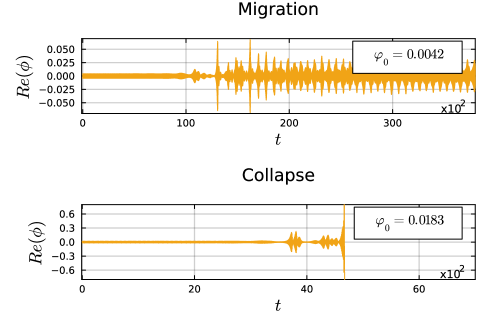
Figure 14: Evolution of the real part of the scalar potential $\phi$ at $r=0$ in for the models with with $\varphi_{0}=0.0042$ (upper panel) and $\varphi_{0}$ = 0.0183 (lower panel). These models illustrate the behavior of the field’s oscillations when the PSs are either migrating to a more stable solution or collapsing to a black hole.

Let us now return to the 4 migrating models with $\varphi_{0}=$ 0.0099, 0.0056, 0.0042 and 0.0023. All these models display irregular oscillations in the central value of the lapse function around some equilibrium position. The total integrated mass at the boundary as a function of time for these models is shown in Figure 15. Here, we again observe a fractional loss of the initial mass due to the fact that some of the field is ejected to infinity (in all these cases approximately 35-39%).

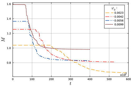
Figure 15: Evolution of the total mass $M$ at the boundary for models in the second excited state that exhibit migration.

We also obtain the FFT of the real part of $\phi$ evaluated at $r=0$ for the initial and final stages of the evolution, see Figure 16. The FFT analysis reveals the frequency spectra from which we can obtain the dominant initial and final frequencies $\omega_{i}$ and $\omega_{f}$. As before, by comparing the total final mass $M_{f}$ and the final dominant frequency $\omega_{f}$ with the families of stationary solutions, we can conclude that the stars are migrating to stable configurations on the ground state, see Figure 17. All the pertinent data for the second excited state is summarized in Table 2 of the Appendix.

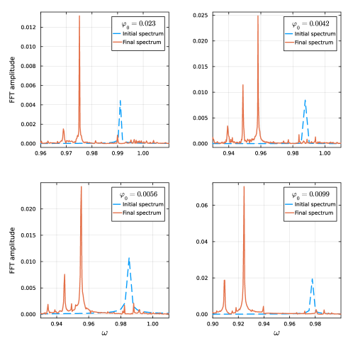
Figure 16: Fourier transform of the time evolution of the real part of $\phi$ evaluated at $r=0$ for those models in the second excited state that exhibit the migration phenomena. These results are similar to those for the first excited state.

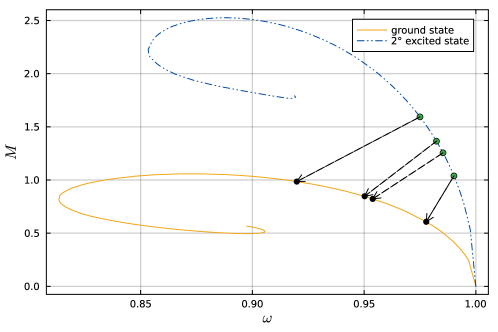
Figure 17: Using the data for the final dominant frequency $\omega_{f}$ and final mass and $M_{f}$ for our migrating models in the second excited state (shown in Table 2 of the Appendix), we can find the final configuration in the ground state family of solutions to which they are migrating.

V Discussion and conclusions

In this paper we have considered families of solutions for excited states of Proca stars in spherical symmetry, with a focus on exploring the dynamical behavior of the first two excited states under perturbations. We considered both the families of stationary solutions, as well as non-linear dynamical simulations of a set of self-consistent perturbed models. Our findings offer valuable insights into the stability and evolution of excited Proca stars, contributing to the further understanding of these compact objects.

It is well known that Proca stars in the ground state are stable against small perturbations for a specific branch corresponding to those configurations with negative binding energy and mass to the left of the maximum mass (minimum binding energy) in the mass versus $\varphi_{0}$ diagram. However, we find that in the case of Proca stars in the first and second excited states this stable branch does not exist. In fact, we find that for excited states only a metastable branch exists for configurations with negative binding energy and low masses. In this metastable branch the Proca stars migrate under perturbations to solutions with lower mass in the stable branch of the ground state, while ejecting excess field to infinity. Our dynamical simulations have allowed us not only to observe the migration phenomena for this type of configurations, but also to determine the final configuration on the ground state to which they are migrating.

For the case of excited states, the absence of dynamically stable Proca stars raises intriguing questions about the factors influencing their instability. Notably, our model does not incorporate self-interactions, which have been demonstrated to play a crucial role in stabilizing excited boson stars [30] and fermion-boson stars [31]. Introducing self-interaction parameters into the model presents an opportunity to further explore the stability and dynamics of excited Proca stars. We are currently in the process of studying this further.

Appendix A Migration data

In Table 2 we present the data corresponding to the models in the first and second excited states that exhibit migration phenomena. We first show the initial values of the frequency $\omega_{i}$ and total mass $M_{i}$ at $t=0$, representing the parameters of the unperturbed stationary configuration. Subsequently, we show the final parameters $\omega_{f}$ and $M_{f}$ at the late stage of our dynamical evolutions, as well as their respective uncertainties due to numerical error. We estimate these uncertainties in $\omega_{f}$ from the width of the peak in the FFT, and in $M_{f}$ from the slow decay of the total mass at the end of our simulations toward an asymptotic value. In the latter case, the uncertainty of $\pm 0.005$ corresponds to the last decimal place for which the value of the mass is still changing, i.e. in all our simulations the third decimal place in the value of $M_{f}$ is still decreasing very slowly at the end, so the asymptotic value should be closer to the lower bound. A comparison of the initial and final parameters reveals notable changes in both the frequency of oscillation of the Proca field and the total integrated mass.

The last two columns in the Table show the frequency $\omega$ and mass $M$ for those solutions in the ground state toward which the perturbed excited solutions seem to be migrating. It is important to mention the fact that the frequencies of the ground state solutions $\omega$ used for the comparisons are not exactly the same as those of the final stage of the migrating solutions $\omega_{f}$. The reason for this is that we do not have solutions for all values of $\omega$ since we have only sampled the solution space for a finite (though large) number of cases, and the frequency is not our free parameter but rather the eigenvalue found at the end. However, we choose those solutions in the ground state that fall within the uncertainty range of $\omega_{f}$.

With these caveats, once we choose the comparison frequency $\omega$ for a fround state solution the corresponding mass $M$ is fixed, and it is remarkable how close it is to the value $M_{f}$ of the migrating solution in each case. This convinces us that the perturbed excited states are indeed migrating to stable solutions on the ground state.

Models	$\omega_{i}$	$M_{i}$	$\omega_{f}\pm\delta\omega_{f}$	$M_{f}\pm$ 0.005	$\omega$	$M$
1° excited	Migration				Initial data: gnd
0.006	0.980	1.042	0.96287 $\pm$ 0.00031	0.769	0.960	0.772
0.009	0.977	1.137	0.95407 $\pm$ 0.00024	0.839	0.953	0.822
0.013	0.973	1.232	0.94499 $\pm$ 0.00026	0.897	0.941	0.898
0.017	0.967	1.322	0.93170 $\pm$ 0.00035	0.955	0.933	0.935
2° excited	Migration				Initial data: gnd
0.0023	0.990	1.038	0.97513 $\pm$ 0.00025	0.655	0.977	0.607
0.0042	0.987	1.255	0.95823 $\pm$ 0.00022	0.811	0.953	0.822
0.0056	0.985	1.364	0.95538 $\pm$ 0.00035	0.829	0.950	0.847
0.0099	0.977	1.593	0.92446 $\pm$ 0.00041	0.981	0.919	0.985

Table 2: Migration phenomena: For the first and second excited states, we show in the first two columns the initial frequency $\omega_{i}$ and initial total mass $M_{i}$ of the corresponding unperturbed configuration. On the third and fourth columns we show the final dominant frequency $\omega_{f}$ and final mass $M_{f}$ after the migration has occurred. The last two columns show the corresponding values for the frequency and mass of configurations on the stable branch of the ground state toward which the dynamical solutions seem to migrate.

References

- Kaup [1968] D. J. Kaup, Phys. Rev. 172, 1331 (1968).
- Ruffini and Bonazzola [1969] R. Ruffini and S. Bonazzola, Phys. Rev. 187, 1767 (1969).
- Brito et al. [2016a] R. Brito, V. Cardoso, C. A. Herdeiro, and E. Radu, Physics Letters B 752, 291 (2016a).
- Finster et al. [1999] F. Finster, J. Smoller, and S.-T. Yau, Phys. Rev. D 59, 104020 (1999), arXiv:gr-qc/9801079 .
- Liebling and Palenzuela [2012] S. L. Liebling and C. Palenzuela, Living Rev.Rel. 15, 6 (2012), arXiv:1202.5809 [gr-qc] .
- Herdeiro and Radu [2020] C. A. R. Herdeiro and E. Radu, Symmetry 12, 2032 (2020), arXiv:2012.03595 [gr-qc] .
- Matos et al. [2000] T. Matos, F. S. Guzman, and L. A. Urena-Lopez, Class. Quantum Grav. 17, 1707 (2000), arXiv:astro-ph/9908152 .
- Matos and Urena-Lopez [2000] T. Matos and L. A. Urena-Lopez, Class. Quantum Grav. 17, L75 (2000), arXiv:astro-ph/0004332 .
- Hu et al. [2000] W. Hu, R. Barkana, and A. Gruzinov, Phys. Rev. Lett. 85, 1158 (2000), arXiv:astro-ph/0003365 .
- Guzman and Rueda-Becerril [2009] F. S. Guzman and J. M. Rueda-Becerril, Phys. Rev. D 80, 084023 (2009), arXiv:1009.1250 [astro-ph.HE] .
- Visinelli [2021] L. Visinelli, Int. J. Mod. Phys. D 30, 2130006 (2021), arXiv:2109.05481 [gr-qc] .
- Brito et al. [2016b] R. Brito, V. Cardoso, C. F. B. Macedo, H. Okawa, and C. Palenzuela, Phys. Rev. D 93, 044045 (2016b), arXiv:1512.00466 [astro-ph.SR] .
- Di Giovanni et al. [2018] F. Di Giovanni, N. Sanchis-Gual, C. A. R. Herdeiro, and J. A. Font, Phys. Rev. D 98, 064044 (2018), arXiv:1803.04802 [gr-qc] .
- Sanchis-Gual et al. [2017] N. Sanchis-Gual, C. Herdeiro, E. Radu, J. C. Degollado, and J. A. Font, Phys. Rev. D 95, 104028 (2017), arXiv:1702.04532 [gr-qc] .
- Zhang et al. [2023] R. Zhang, L.-X. Huang, and Y.-Q. Wang, (2023), arXiv:2312.15755 [gr-qc] .
- Salazar Landea and García [2016] I. Salazar Landea and F. García, Phys. Rev. D 94, 104006 (2016), arXiv:1608.00011 [hep-th] .
- Lazarte and Alcubierre [2024] C. Lazarte and M. Alcubierre, Class. Quant. Grav. 41, 135003 (2024).
- Alcubierre [2008] M. Alcubierre, Introduction to Numerical Relativity (Oxford Univ. Press, New York, 2008).
- Shibata and Nakamura [1995] M. Shibata and T. Nakamura, Phys. Rev. D52, 5428 (1995).
- Baumgarte and Shapiro [1998] T. W. Baumgarte and S. L. Shapiro, Phys. Rev. D59, 024007 (1998), gr-qc/9810065 .
- Alcubierre and Mendez [2011] M. Alcubierre and M. D. Mendez, Gen.Rel.Grav. 43, 2769 (2011), arXiv:1010.4013 [gr-qc] .
- Alcubierre and Torres [2015] M. Alcubierre and J. M. Torres, Class. Quant. Grav. 32, 035006 (2015), arXiv:1407.8529 [gr-qc] .
- Alcubierre et al. [2019] M. Alcubierre, J. Barranco, A. Bernal, J. C. Degollado, A. Diez-Tejedor, M. Megevand, D. Núñez, and O. Sarbach, Class. Quant. Grav. 36, 215013 (2019), arXiv:1906.08959 [gr-qc] .
- Degollado et al. [2020] J. C. Degollado, M. Salgado, and M. Alcubierre, Phys. Lett. B 808, 135666 (2020), arXiv:2008.10683 [gr-qc] .
- Jiménez-Vázquez and Alcubierre [2022a] E. Jiménez-Vázquez and M. Alcubierre, Physical Review D 105, 10.1103/physrevd.105.064071 (2022a).
- Jiménez-Vázquez and Alcubierre [2022b] E. Jiménez-Vázquez and M. Alcubierre, Physical Review D 106, 10.1103/physrevd.106.044071 (2022b).
- Brito et al. [2016c] R. Brito, V. Cardoso, C. A. R. Herdeiro, and E. Radu, Phys. Lett. B 752, 291 (2016c), arXiv:1508.05395 [gr-qc] .
- Herdeiro et al. [2017] C. A. R. Herdeiro, A. M. Pombo, and E. Radu, Phys. Lett. B 773, 654 (2017), arXiv:1708.05674 [gr-qc] .
- Cardoso and Pani [2019] V. Cardoso and P. Pani, Living Rev. Rel. 22, 4 (2019), arXiv:1904.05363 [gr-qc] .
- Brito et al. [2023] M. Brito, C. Herdeiro, E. Radu, N. Sanchis-Gual, and M. Zilhão, Phys. Rev. D 107, 084022 (2023), arXiv:2302.08900 [gr-qc] .
- Di Giovanni et al. [2021] F. Di Giovanni, S. Fakhry, N. Sanchis-Gual, J. C. Degollado, and J. A. Font, Class. Quant. Grav. 38, 194001 (2021), arXiv:2105.00530 [gr-qc] .