Geometrical-optics analysis of the interaction between light and gravitational waves from binaries

Abstract

We consider a situation in which light emitted from the neighborhood of a binary interacts with gravitational waves from the binary (e.g., a supermassive black hole binary in a quasar, a binary pulsar, etc.). The effect is cumulative over the long path lengths of light propagation and might be appreciable if the interaction initially takes place close to the source of gravitational waves, where the strain amplitude can be large. This situation can be modeled effectively using spherical gravitational waves (i.e., transverse-traceless radially propagating waves), with the strain amplitude varying with the distance from the source to a field point where the two wavefronts of light and gravitational waves meet each other. Our analysis employs geometrical-optics methods in curved spacetime, where the curvature is due to gravitational waves propagating in a flat spacetime background. We place a particular focus on the effect of gravitational Faraday rotation (or Skrotskii/Rytov effect) resulting from the interaction between light and gravitational waves from binaries.

1 Introduction

Astronomers use light, i.e., electromagnetic waves (EMWs), to make observations of a wide variety of astrophysical events. Among others, recently, light has been used as a major tool to detect gravitational waves (GWs), due to its prominent property – interaction with other kinds of waves; e.g., the property is exploited by the detection schemes via laser interferometers – LIGO, VIRGO, GEO600, KAGRA, LIGO-India, eLISA, etc. PhysRevLett.116.061102 ; Grote_2010 ; Somiya_2012 ; LIGO-India_2011 ; amaroseoane_2012 and via pulsar timing arrays – EPTA, PPTA, IPTA, SKA, etc. Kramer_2013 ; Hobbs_2013 ; Manchester_2013 ; Dewdney_2009 .

Two massive objects orbiting each other (e.g., a black hole (BH) binary, a neutron star (NS) binary, a BH-NS binary, etc.) generate GWs, which propagate radially in all directions, with the energy of GWs decreasing over the distance from the source. However, when reaching a distant observer (like ones located at those aforementioned detectors), the energy of GWs decreases considerably, and the (strain) amplitude is usually treated as an extremely small constant value; therefore, the effects on EMWs due to GWs are extremely small too, of the same order as the strain amplitude.

In case light is emitted from the neighborhood of a binary (e.g., a supermassive BH binary in a quasar, a binary pulsar, etc.) at the same time GWs are emitted from the binary, the EMWs interact with the GWs all along the propagation path towards an observer. Here the strain amplitude varies with the distance from the binary source to a field point of GWs, where the two wavefronts of EMWs and GWs cross each other.

A number of studies have been published in the context of the interaction between EMWs and plane GWs. Among others, Halilsoy and Gurtug Halilsoy_2007 analyzed the Faraday rotation in the polarization vector of a linearly polarized electromagnetic shock wave upon encountering with GWs. Hacyan Hacyan_2012 ; Hacyan_2016 determined the influence of a GW on the elliptic polarization of light, deducing the rotation of the polarization angle and the corresponding Stokes parameters, and applied this effect to the detection of GWs, as a complement to the pulsar timing method. Cabral and Lobo Cabral_2017 obtained electromagnetic field oscillations induced by GWs, and found that these lead to the presence of longitudinal modes and dynamical polarization patterns of electromagnetic radiation. Park and Kim Park_2021 employed the perturbation theory of general relativity to analyze the influence of GWs on EMWs, concentrating mainly on the effects on the polarization of light, and applied their analysis to the observation of GWs by means of Stokes parameters. Kim and Park Kim_2021 investigated how light is perturbed in the presence of GWs from a general relativistic perspective, by solving Maxwell’s equations in the geometrical-optics limit.

In the aforementioned works, the interaction between EMWs and GWs is assumed to take place far away from the source of GWs; therefore, the strain amplitude of GWs can be treated as an extremely small constant value. In contrast with them, Cruise Cruise_1983 estimated the rotation angle of the plane of polarization of an EMW, which results from the passage of the wave through a non-flat spacetime with a GW present. Here the EMW-GW interaction can occur close to the GW source and continue all along the EMW propagation path towards an observer. In this case, the strain amplitude can be initially large and decreases inversely as the distance from the source to a point of EMW-GW intersection; as a result, the cumulative effect from EMW-GW interaction over the long propagation path can be outstanding in comparison with all the aforementioned cases, in which EMWs interact with plane GWs. However, despite a fresh perspective on the problem, Cruise Cruise_1983 overlooked some other important aspects: the spherical property of the GW, i.e., the dependence of the wave’s amplitude and phase on $\left(r,\theta,\phi\right)$ in spherical polar coordinates, and its influence on EMW-GW interaction. Besides, he used several simplifying assumptions, with which to make his analysis easier, and this inevitably led to some loss of generality in his approach.

In this paper, we investigate the interaction between EMWs and GWs, and its effects on the properties of light, in a situation where light emitted from the neighborhood of a binary meets GWs from the binary all along the way to an observer. To this end, the paper proceeds largely in two steps as follows. In Sect. 2, we will model the situation effectively using spherical GWs, and perform a geometrical-optics analysis in curved spacetime, with the curvature being due to the GWs propagating in flat spacetime. In Sect. 3, for application of our analysis, we will focus in particular on the effect of gravitational Faraday rotation (or Skrotskii/Rytov effect), resulting from the interaction between EMWs and GWs from binaries, such as a supermassive BH binary in quasar and a double NS system.

2 EMWs propagating through the GW background

2.1 Spacetime with spherical GWs

Suppose a binary system of two masses $M_{1}$ and $M_{2}$ moving around each other in an orbit. Then transverse-traceless (TT) radially propagating GWs from this source are expressed as

$$h_{ij}^{\mathrm{TT}}=\frac{2G}{c^{4}r}\left(P_{i}^{\,k}P_{j}^{\,l}-\frac{1}{2}P_{ij}P^{kl}\right)\ddot{Q}_{kl}\left(t_{\mathrm{R}}\right),$$ (1)

where the Latin indices $i$, $j$, $\ldots$ refer to the spatial coordinates, and $G\approx 6.6743\times 10^{-11}\,\mathrm{m^{3}\,kg^{-1}\,s^{-2}}$ is the gravitational constant, and $c\approx 2.998\times 10^{8}\,\mathrm{m\,s^{-1}}$ is the speed of light, and $P^{ij}=\delta^{ij}-n^{i}n^{j}$ is the transverse projection tensor, and

$$Q^{ij}=\mu X^{i}X^{j}-\frac{1}{3}\delta^{ij}\left(\mu X^{k}X_{k}\right),$$ (2)

denotes the mass quadrupole moment of the system, with $\mu\equiv M_{1}M_{2}/(M_{1}+M_{2})$ being the reduced mass and $\mathbf{X}\equiv\mathbf{r}_{1}-\mathbf{r}_{2}$ referring to the relative coordinates of the two bodies, and $t_{\mathrm{R}}=t-\mathbf{n}\cdot\mathbf{r}/c$ is the retarded time.

In a suitably chosen frame, the nonzero components of the quadrupole moment (2) are obtained for a circular orbit:

$$Q_{xx} = \mu R_{\mathrm{o}}^{2}\left[\cos^{2}\left(\Omega t\right)-\frac{1}{3}\right],$$ (3)

$$Q_{yy} = \mu R_{\mathrm{o}}^{2}\left[\sin^{2}\left(\Omega t\right)-\frac{1}{3}\right],$$ (4)

$$Q_{xy} = Q_{yx}=\mu R_{\mathrm{o}}^{2}\cos\left(\Omega t\right)\sin\left(\Omega t\right),$$ (5)

$$Q_{zz} = -\frac{\mu R_{\mathrm{o}}^{2}}{3},$$ (6)

where $R_{\mathrm{o}}=\left|\mathbf{X}\right|$ is the radius of the orbit, and $\Omega=\sqrt{G(M_{1}+M_{2})/R_{\mathrm{o}}^{3}}$ is the orbital angular velocity. Now, choosing $\mathbf{n}=\mathbf{e}_{r}=\left(\sin\theta\cos\phi,\sin\theta\sin\phi,\cos\theta\right)$ for $P^{ij}=\delta^{ij}-n^{i}n^{j}$ and $t_{\mathrm{R}}=t-\mathbf{n}\cdot\mathbf{r}/c$, one can work out all the components of the GWs from (1) in the Cartesian coordinate frame $\left(\mathbf{e}_{x},\mathbf{e}_{y},\mathbf{e}_{z}\right)$:

$$h_{xx}^{\mathrm{TT}} =\mathcal{H}\left(r\right)\left[-\cos^{2}\theta\cos\left(-\omega_{\mathrm{g}}t+kr\right)+\frac{1}{2}\sin^{2}\theta\left(1-\sin^{2}\theta\cos^{2}\phi\right)\cos\left(-\omega_{\mathrm{g}}t+kr+2\phi\right)\right],$$ (7)

$$h_{xy}^{\mathrm{TT}} =\mathcal{H}\left(r\right)\left[\cos^{2}\theta\sin\left(-\omega_{\mathrm{g}}t+kr\right)-\frac{1}{4}\sin^{4}\theta\sin\left(2\phi\right)\cos\left(-\omega_{\mathrm{g}}t+kr+2\phi\right)\right],$$ (8)

$$h_{xz}^{\mathrm{TT}} =\mathcal{H}\left(r\right)\left[\sin\theta\cos\theta\cos\left(-\omega_{\mathrm{g}}t+kr+\phi\right)-\frac{1}{2}\sin^{3}\theta\cos\theta\cos\phi\cos\left(-\omega_{\mathrm{g}}t+kr+2\phi\right)\right],$$ (9)

$$h_{yy}^{\mathrm{TT}} =\mathcal{H}\left(r\right)\left[\cos^{2}\theta\cos\left(-\omega_{\mathrm{g}}t+kr\right)+\frac{1}{2}\sin^{2}\theta\left(1-\sin^{2}\theta\sin^{2}\phi\right)\cos\left(-\omega_{\mathrm{g}}t+kr+2\phi\right)\right],$$ (10)

$$h_{yz}^{\mathrm{TT}} =\mathcal{H}\left(r\right)\left[-\sin\theta\cos\theta\sin\left(-\omega_{\mathrm{g}}t+kr+\phi\right)-\frac{1}{2}\sin^{3}\theta\cos\theta\sin\phi\cos\left(-\omega_{\mathrm{g}}t+kr+2\phi\right)\right],$$ (11)

$$h_{zz}^{\mathrm{TT}} =\mathcal{H}\left(r\right)\left[-\frac{1}{2}\sin^{2}\theta\left(1+\cos^{2}\theta\right)\cos\left(-\omega_{\mathrm{g}}t+kr+2\phi\right)\right],$$ (12)

where $\mathcal{H}\left(r\right)\equiv G\mu R_{\mathrm{o}}^{2}\omega_{\mathrm{g}}^{2}/\left(c^{4}r\right)$ represents the radially varying strain amplitude and $\omega_{\mathrm{g}}\equiv 2\Omega=2\sqrt{G(M_{1}+M_{2})/R_{\mathrm{o}}^{3}}$ denotes the GW frequency.

Now, the spacetime geometry, in which Maxwell’s equations are solved, reads

$$ds^{2}= -c^{2}dt^{2}+\left(1+h_{xx}^{\mathrm{TT}}\right)dx^{2}+2h_{xy}^{\mathrm{TT}}dxdy+2h_{xz}^{\mathrm{TT}}dxdz$$

$$+\left(1+h_{yy}^{\mathrm{TT}}\right)dy^{2}+2h_{yz}^{\mathrm{TT}}dydz+\left(1+h_{zz}^{\mathrm{TT}}\right)dz^{2},$$ (13)

where the components of $h_{ij}^{\mathrm{TT}}$ refer to (7)-(12). Then it is implied that our solutions to the Maxwell’s equations defined in this spacetime geometry naturally contain the interaction between EMWs and GWs.

One should note that transforming the GWs as given by (7)-(12) above from the Cartesian coordinate frame $\left(\mathbf{e}_{x},\mathbf{e}_{y},\mathbf{e}_{z}\right)$ to the spherical coordinate frame $(\mathbf{e}_{r},\mathbf{e}_{\hat{\theta}},\mathbf{e}_{\hat{\phi}})$ yields the compact expressions of ‘spherical’ GWs from the binary source Maggiore_2007 ; thorne2017modern :

$$h_{+}\left(t,r,\theta,\phi\right) \equiv h_{\hat{\theta}\hat{\theta}}^{\mathrm{TT}}=-h_{\hat{\phi}\hat{\phi}}^{\mathrm{TT}}$$

$$=-\mathcal{H}\left(r\right)\left(\frac{1+\cos^{2}\theta}{2}\right)\cos\left(-\omega_{\mathrm{g}}t+kr+2\phi\right),$$ (14)

$$h_{\times}\left(t,r,\theta,\phi\right) \equiv h_{\hat{\theta}\hat{\phi}}^{\mathrm{TT}}=h_{\hat{\phi}\hat{\theta}}^{\mathrm{TT}}$$

$$=\mathcal{H}\left(r\right)\cos\theta\sin\left(-\omega_{\mathrm{g}}t+kr+2\phi\right),$$ (15)

where the subscript indices $\hat{\theta}$ and $\hat{\phi}$ denote the basis vectors $\mathbf{e}_{\hat{\theta}}$ and $\mathbf{e}_{\hat{\phi}}$, respectively.

2.2 Geometrical-optics analysis for EMWs in the GW background

Light (EMWs) propagating in a spacetime curved due to GWs, as given in Sect. 2.1, can be described by Maxwell’s equations:

$$\square A^{\mu}-R^{\mu}{}_{\nu}A^{\nu}=0,$$ (16)

where the Greek indices $\mu$, $\nu$, $\ldots$ refer to the temporal and spatial coordinates, and $\square A^{\mu}\equiv g^{\nu\rho}\nabla_{\nu}\nabla_{\rho}A^{\mu}$ means the d’Alembertian on a vector potential and, $R_{\mu\nu}$ denotes the Ricci tensor. Here both the operator and the tensor are defined in the spacetime geometry as given by Eq. (13), and therefore expressed in terms of $h_{ij}^{\mathrm{TT}}$. However, in Lorenz gauge ($\partial^{\mu}\bar{h}_{\mu\nu}=0$) and TT gauge ($h_{0\mu}=0$ and $h_{\,\,\,\mu}^{\mu}=0$), it turns out

$$R_{\mu\nu}=\mathcal{O}\left(h^{2}\right).$$ (17)

Therefore, the Maxwell’s equations (16) reduce to

$$\square A^{\mu}=\mathcal{O}\left(h^{2}\right).$$ (18)

We consider a geometrical-optics ansatz for Eq. (18) poisson2014gravity ; dolan2018geometrical :

$$A^{\mu}\left(x\right)=\mathcal{A}\left(x\right)\varepsilon^{\mu}\left(x\right)\exp\left(\mathrm{i}\varpi\Psi\left(x\right)\right),$$ (19)

where $\mathcal{A}\left(x\right)$ is the amplitude, $\varepsilon^{\mu}\left(x\right)$ denotes the polarization vector, and $\exp\left(\mathrm{i}\varpi\Psi\left(x\right)\right)$ represents the wave field, with $\varpi$ being a dimensionless parameter. Plugging this into the Maxwell’s equations (18), we obtain

$$(i) -{\,{\varpi^{2}\left(K^{\nu}K_{\nu}\mathcal{A}\varepsilon^{\mu}\right)}}$$

$${(ii)} {+\,\mathrm{i}{\varpi^{1}}\left[\varepsilon^{\mu}{\nabla_{\nu}\left(\mathcal{A}^{2}K^{\nu}\right)}+2\mathcal{A}{K^{\nu}\nabla_{\nu}\varepsilon^{\mu}}\right]}$$

$$(iii) +\,\mathcal{O}\left(\varpi^{0}\right)=0,$$ (20)

where $\varpi$ serves as an order-counting parameter and $K^{\mu}\equiv\nabla^{\mu}\Psi$ denotes the wave vector of EMWs.

From the null condition $K^{\mu}K_{\mu}=0$ (which makes the term (i) in Eq. (20) vanish) and with the term (ii) in Eq. (20) vanishing, we find

$${K^{\nu}\nabla_{\nu}K^{\mu}=0} (\mathrm{geodesic\;equation}),$$ (21)

$${\nabla_{\nu}\left(\mathcal{A}^{2}K^{\nu}\right)=0} (\mathrm{conservation\;of\;flux}),$$ (22)

$${K^{\nu}\nabla_{\nu}\varepsilon^{\mu}=0} (\mathrm{Skrotskii/Rytov\;effect}).$$ (23)

Solving these equations, we obtain

$${\delta K_{[1]}^{\mu}} \simeq{-K_{\left[0\right]}^{\nu}\int(K_{\left[0\right]}^{\rho}k_{\rho}){\tilde{h}^{\mathrm{s}}{}_{\,\,\,\nu}^{\mu}}\mathrm{d}\lambda+\frac{K_{\left[0\right]}^{\nu}K_{\left[0\right]}^{\rho}}{2}\int k^{\mu}{\tilde{h}_{\nu\rho}^{\mathrm{s}}}\mathrm{d}\lambda},$$ (24)

$${\delta\Psi_{[1]}} \simeq{-\frac{K_{\left[0\right]}^{\mu}K_{\left[0\right]}^{\nu}}{2}\int\left[\int(K_{\left[0\right]}^{\rho}k_{\rho}){\tilde{h}_{\mu\nu}^{\rm{s}}}\mathrm{d}\lambda\right]\mathrm{d}\lambda},$$ (25)

$${\delta\mathcal{A}_{[1]}} \simeq{0},$$ (26)

$${\delta\varepsilon_{[1]}^{\mu}} \simeq{-\frac{\varepsilon_{\left[0\right]}^{\nu}}{2}\int(K_{\left[0\right]}^{\rho}k_{\rho}){\tilde{h}^{\rm{s}}{}_{\,\,\,\nu}^{\mu}}\mathrm{d}\lambda-\frac{K_{\left[0\right]}^{\nu}}{2}\int(\varepsilon_{\left[0\right]}^{\rho}k_{\rho}){\tilde{h}^{\mathrm{s}}{}_{\,\,\,\nu}^{\mu}}\mathrm{d}\lambda+\frac{K_{\left[0\right]}^{\nu}\varepsilon_{\left[0\right]}^{\rho}}{2}\int k^{\mu}{\tilde{h}_{\nu\rho}^{\mathrm{s}}}\mathrm{d}\lambda},$$ (27)

where we have assumed a perturbative solution for each quantity, i.e., $K^{\mu}=K_{[0]}^{\mu}+\delta K_{[1]}^{\mu}+\mathcal{O}\left(h^{2}\right)$, $\Psi=\Psi_{[0]}+\delta\Psi_{[1]}+\mathcal{O}\left(h^{2}\right)$ (c.f. $K_{[0]}^{\mu}=\nabla^{\mu}\Psi_{[{0}]}$), $\mathcal{A}=\mathcal{A}_{[{0}]}+\delta\mathcal{A}_{[{1}]}+\mathcal{O}\left(h^{2}\right)$ and $\varepsilon^{\mu}=\varepsilon_{[{0}]}^{\mu}+\delta\varepsilon_{[{1}]}^{\mu}+\mathcal{O}\left(h^{2}\right)$, with the subscripts $[0]$ and $[1]$ meaning ‘unperturbed’ and ‘first-order in $h$’, respectively, and $\lambda$ is an affine parameter defined via $\mathrm{d}x^{\mu}/\mathrm{d}\lambda=K_{\left[{0}\right]}^{\mu}$. Here we have renamed and redefined $h_{\mu\nu}^{\mathrm{TT}}$ from Eqs. (7)-(12):

$$h_{\mu\nu}^{\mathrm{s}} =\Re\left(\mathfrak{H}_{\mu\nu}\left(r,\theta,\phi\right)\exp\left(\mathrm{i}k_{\alpha}x^{\alpha}\right)\right),$$ (28)

$$\tilde{h}_{\mu\nu}^{\mathrm{s}} =\Re\left(\mathrm{i}\mathfrak{H}_{\mu\nu}\left(r,\theta,\phi\right)\exp\left(\mathrm{i}k_{\alpha}x^{\alpha}\right)\right),$$ (29)

where the label ‘$\mathrm{TT}$’ (meaning transverse-traceless) has been replaced by ‘$\mathrm{s}$’ (meaning spherical), and $\mathfrak{H}_{\mu\nu}\left(r,\theta,\phi\right)$ represents the complex strain tensor, which can be read off from (7)-(12). Note that ‘$\simeq$’ signs in (24)-(27) above are due to $\partial^{\mu}h_{\nu\rho}^{\mathrm{s}}\simeq k^{\mu}\tilde{h}_{\nu\rho}^{\mathrm{s}}$.

Finally, our solutions to Eq. (18) are given by means of (19), in a perturbative form:

$$A^{\mu}\left(x\right)=\mathcal{A}_{[0]}\left[\varepsilon_{[0]}^{\mu}+{\delta\varepsilon_{[1]}^{\mu}\left(x\right)}\right]\exp\left(\mathrm{i}\left(K_{\alpha[{0}]}x^{\alpha}+\delta\Psi_{[1]}\left(x\right)\right)\right),$$ (30)

where $\delta\Psi_{[1]}$ and $\delta\varepsilon_{[1]}^{\mu}$ refer to Eqs. (25) and (27), respectively. In reference to (30) together with (24)-(27), one should note the following: based on the geometrical-optics analysis, we have first-order modulations of the phase, the wave vector and the polarization vector of EMWs due to GWs, with the exception of the amplitude, and our solutions to the Maxwell’s equations are expressed in terms of such modulations.

3 Applications for EMW-GW interaction: (1) Supermassive BH binary in quasar, (2) Double neutron star system

3.1 Binaries and GWs

As a good example for the EMW-GW interaction, one can consider quasars, the brilliant cores of active galaxies, as they may commonly host two central supermassive BHs, which fall into an orbit about one another as a result of the merger between two galaxies; e.g., Markarian 231 (Mrk 231), the nearest galaxy to Earth that hosts a quasar, has been found to be powered by two such BHs, using NASA’s Hubble Space Telescope. The binary BHs generate a tremendous amount of energy that makes the core of the host galaxy outshine the glow of its population of billions of stars Yan_2015 ; Hubble2015 . At the same time, light from a quasar will interact with GWs emitted by the binary. In this situation, however, the GW strain amplitude $h$ is not treated as a constant value; rather, it varies with the distance $r$ from the source to a field point where the two wavefronts of the light and the GWs meet each other. Therefore, the interaction between the light and the GWs weakens as $h$ decreases over the distance, but accumulates over the entire path of light propagation.

Neutron star (NS) binaries are another example we can take from which to investigate the EMW-GW interaction. For instance, PSR J1913+16 is known as the first double neutron star (DNS) system, discovered by Hulse and Taylor in 1974 Hulse_1975 . This binary system consists of a pulsar and a massive companion orbiting around each other, gravitational interactions of which can be indirectly verified via its orbital contraction, caused by the energy loss of the system emitting GWs. There are 19 DNS systems that have been discovered until now (as of 2020), and amongst them, PSR J0737–3039 is the only one known to possess both the primary and the companion NSs detected as pulsars Burgay_2003 ; Lyne_2004 ; Liu_2021 . Likewise, as $h$ decreases over the distance, the interaction between the pulsar emissions and the GWs weakens, but accumulates over the entire path of light propagation.

3.2 Faraday rotation (Skrotskii/Rytov effect) by GWs

Among the effects due to GWs, we focus on the Faraday rotation of the polarization vector of EMWs. Recalling from Sect. 2.2, the first-order modulation of the polarization vector due to GWs is given by

$$K^{\nu}\nabla_{\nu}\varepsilon^{\mu} =0\;\;\;(\mathrm{Skrotskii/Rytov\;effect})$$

$$\Rightarrow\;\;{\delta\varepsilon_{[{1}]}^{\mu}} \simeq{-\frac{\varepsilon_{\left[{0}\right]}^{\nu}}{2}\int(K_{\left[{0}\right]}^{\rho}k_{\rho}){\tilde{h}^{\rm{s}}{}_{\,\,\,\nu}^{\mu}}\mathrm{d}\lambda-\frac{K_{\left[{0}\right]}^{\nu}}{2}\int(\varepsilon_{\left[{0}\right]}^{\rho}k_{\rho}){\tilde{h}^{\rm{s}}{}_{\,\,\,\nu}^{\mu}}\mathrm{d}\lambda+\frac{K_{\left[{0}\right]}^{\nu}\varepsilon_{\left[{0}\right]}^{\rho}}{2}\int k^{\mu}{\tilde{h}_{\nu\rho}^{\mathrm{s}}}\mathrm{d}\lambda}.$$ (31)

Then using this, the Faraday rotation angle can be computed as

$$\varphi_{\mathrm{F}}\equiv\cos^{-1}\left(\boldsymbol{\varepsilon}_{\left[0\right]}\cdot\boldsymbol{\hat{\varepsilon}}\right)\approx\sqrt{\delta\boldsymbol{\varepsilon}_{\left[1\right]}^{2}-\left(\boldsymbol{\varepsilon}_{\left[0\right]}\cdot\delta\boldsymbol{\varepsilon}_{\left[1\right]}\right)^{2}}+\mathcal{O}\left(h^{2}\right).$$ (32)

Now, without loss of generality, we may set $\phi_{\star}=0$ for the angular coordinates $\left(\theta_{\star},\phi_{\star}\right)$ of the spatial propagation vector of our quasar’s light (as represented by the orange dashed line in Figure1):

$$\mathbf{K}_{\left[0\right]}=\frac{\omega_{\mathrm{e}}}{c}\left(\sin\theta_{\star},0,\cos\theta_{\star}\right).$$ (33)

In the Coulomb gauge, however, a polarization vector associated with this can be written as

$$\boldsymbol{\varepsilon}_{\left[0\right]}=\left(\cos\theta_{\star},0,-\sin\theta_{\star}\right).$$ (34)

Then from Eq. (32) one finds

$$\varphi_{\mathrm{F}} \approx\sqrt{\sin^{2}\theta_{\star}\left(\delta\varepsilon^{x}_{\left[1\right]}\right)^{2}+2\cos\theta_{\star}\sin\theta_{\star}\delta\varepsilon^{x}_{\left[1\right]}\delta\varepsilon^{z}_{\left[1\right]}+\cos^{2}\theta_{\star}\left(\delta\varepsilon^{z}_{\left[1\right]}\right)^{2}}$$

$$=\frac{c}{\omega_{\mathrm{e}}}\left|\mathbf{K}_{\left[0\right]}\cdot\delta\boldsymbol{\varepsilon}_{\left[1\right]}\right|.$$ (35)

Using Eq. (31), the expression (35) can be specified in terms of GWs:

$$\varphi_{\mathrm{F}} \approx\left|\frac{K_{\left[{0}\right]}^{\mu}K_{\left[{0}\right]}^{\nu}}{2}\int^{\lambda_{\mathrm{f}}}_{\lambda_{\mathrm{i}}}\left(\varepsilon_{\left[{0}\right]}^{\rho}k_{\rho}\right){\tilde{h}^{\mathrm{s}}_{\mu\nu}}\mathrm{d}\lambda\right|$$

$$=\frac{\omega_{\mathrm{e}}}{2c}\left|\sin^{2}\theta_{\star}\int^{\lambda_{\mathrm{f}}}_{\lambda_{\mathrm{i}}}\left(\boldsymbol{\varepsilon}_{\left[0\right]}\cdot\mathbf{k}\right)\tilde{h}_{xx}^{\mathrm{s}}\mathrm{d}\lambda+2\cos\theta_{\star}\sin\theta_{\star}\int^{\lambda_{\mathrm{f}}}_{\lambda_{\mathrm{i}}}\left(\boldsymbol{\varepsilon}_{\left[0\right]}\cdot\mathbf{k}\right)\tilde{h}_{xz}^{\mathrm{s}}\mathrm{d}\lambda\right.$$

$$\left.+\cos^{2}\theta_{\star}\int^{\lambda_{\mathrm{f}}}_{\lambda_{\mathrm{i}}}\left(\boldsymbol{\varepsilon}_{\left[0\right]}\cdot\mathbf{k}\right)\tilde{h}_{zz}^{\mathrm{s}}\mathrm{d}\lambda\right|.$$ (36)

where $\boldsymbol{\varepsilon}_{\left[0\right]}$ refers to (34) and

$$\mathbf{k}=\frac{\omega_{\mathrm{g}}}{c}\left(\sin\theta\cos\phi,\sin\theta\sin\phi,\cos\theta\right),$$ (37)

and in view of (7)-(12), (28) and (29) one can write out the components of GWs:

$${{{\tilde{h}_{xx}^{\mathrm{s}}}}} {=}{\mathcal{H}\left(r\right)\left[\cos^{2}\theta\sin\left(-\omega_{\mathrm{g}}t+kr\right)-\frac{1}{2}\sin^{2}\theta\left(1-\sin^{2}\theta\cos^{2}\phi\right)\sin\left(-\omega_{\mathrm{g}}t+kr+2\phi\right)\right]},$$ (38)

$${{{\tilde{h}_{xz}^{\mathrm{s}}}}} {=}{\mathcal{H}\left(r\right)\left[-\sin\theta\cos\theta\sin\left(-\omega_{\mathrm{g}}t+kr+\phi\right)+\frac{1}{2}\sin^{3}\theta\cos\theta\cos\phi\sin\left(-\omega_{\mathrm{g}}t+kr+2\phi\right)\right]},$$ (39)

$${{{\tilde{h}_{zz}^{\mathrm{s}}}}} {=}{\mathcal{H}\left(r\right)\left[\frac{1}{2}\sin^{2}\theta\left(1+\cos^{2}\theta\right)\sin\left(-\omega_{\mathrm{g}}t+kr+2\phi\right)\right]},$$ (40)

where $\mathcal{H}\left(r\right)=G\mu R_{\mathrm{o}}^{2}\omega_{\mathrm{g}}^{2}/\left(c^{4}r\right)$.

For evaluation of the Faraday rotation angle in Eq. (36) above, one can express the following quantities, all in terms of a single parameter $\xi\equiv\tan\left(\gamma/2\right)$, where $\gamma$ denotes the angle between the propagation directions of light and GWs (see Fig. 1 and Appendix A for details):

$$r=\frac{r_{\mathrm{eq}}\sqrt{1-\sin^{2}\theta_{\star}\cos^{2}\varphi}\left(1+\xi^{2}\right)}{2\xi},$$ (41)

$$\sin\theta\cos\phi={\frac{2\cos^{2}\theta_{\star}\cos\varphi\xi}{\sqrt{1-\sin^{2}\theta_{\star}\cos^{2}\varphi}\left(1+\xi^{2}\right)}+\frac{\sin\theta_{\star}\left(1-\xi^{2}\right)}{1+\xi^{2}}},$$ (42)

$$\sin\theta\sin\phi={\frac{2\sin\varphi\xi}{\sqrt{1-\sin^{2}\theta_{\star}\cos^{2}\varphi}\left(1+\xi^{2}\right)}},$$ (43)

$$\cos\theta={\frac{\cos\theta_{\star}\left(1-\xi^{2}\right)}{1+\xi^{2}}-\frac{2\cos\theta_{\star}\sin\theta_{\star}\cos\varphi\xi}{\sqrt{1-\sin^{2}\theta_{\star}\cos^{2}\varphi}\left(1+\xi^{2}\right)}},$$ (44)

$$\boldsymbol{\varepsilon}_{\left[0\right]}\cdot\mathbf{k}=\frac{2\omega_{\mathrm{g}}\cos\theta_{\star}\cos\varphi\xi}{c\sqrt{1-\sin^{2}\theta_{\star}\cos^{2}\varphi}\left(1+\xi^{2}\right)},$$ (45)

$$\left.\left(-\omega_{\mathrm{g}}t+kr\right)\right|_{\mathrm{photon\,path}}=-\omega_{\mathrm{g}}t_{0}+\frac{\omega_{\mathrm{g}}r_{\mathrm{eq}}\sqrt{1-\sin^{2}\theta_{\star}\cos^{2}\varphi}\xi}{c},$$ (46)

$$\mathrm{d}\lambda=\frac{\left.\mathrm{d}\left(k_{\mu}x^{\mu}\right)\right|_{\mathrm{photon\,path}}}{K_{\left[{0}\right]}^{\nu}k_{\nu}}=\frac{\left.\mathrm{d}\left(-\omega_{\mathrm{g}}t+kr\right)\right|_{\mathrm{photon\,path}}}{-c^{-2}\omega_{\mathrm{e}}\omega_{\mathrm{g}}+\mathbf{K}_{\left[0\right]}\cdot\mathbf{k}}$$

$$=-\frac{cr_{\mathrm{eq}}\sqrt{1-\sin^{2}\theta_{\star}\cos^{2}\varphi}\left(1+\xi^{2}\right)}{2\omega_{\mathrm{e}}\xi^{2}}\mathrm{d}\xi,$$ (47)

where the expressions in Eqs. (41)-(44) have been derived from the oblique cylinder as depicted in Fig. 1, using the relations $\cos\gamma=\left(1-\xi^{2}\right)/\left(1+\xi^{2}\right)$ and $\sin\gamma=2\xi/\left(1+\xi^{2}\right)$ (see Appendix A for details of derivations), and in Eqs. (45) and (47) $\boldsymbol{\varepsilon}_{\left[0\right]}$, $\mathbf{k}$ and $\mathbf{K}_{\left[0\right]}$ refer to (34), (37) and (33), respectively, and in Eqs. (46) and (47) $t=t_{0}+r\cos\gamma/c$ along the photon path, and due to the substitution $\mathrm{d}\lambda\rightarrow\mathrm{d}\xi$, the limits of integration in Eq. (36) should change: $\lambda_{\mathrm{i}}\rightarrow\xi_{\mathrm{i}}=\sqrt{\left(1-\sin\theta_{\star}\cos\varphi\right)/\left(1+\sin\theta_{\star}\cos\varphi\right)}$ and $\lambda_{\mathrm{f}}\rightarrow\xi_{\mathrm{f}}=0$

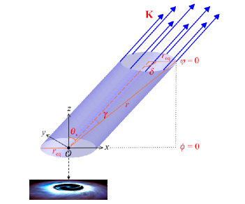
Figure 1: Oblique cylinder: $\left(x-z\tan\theta_{\star}\right)^{2}+y^{2}=r_{\mathrm{eq}}^{2}$. A black hole binary as a source of GWs is located at the origin $O$. Consider a circular ring of radius $r_{\mathrm{eq}}$ encircling the binary on the equatorial plane, from which light beams propagate along the direction, tilted by an angle $\theta_{\star}$ from the normal to the plane. The interaction between the quasar’s light and the GWs can be described as occurring on the surface of an oblique cylinder with the radius $r_{\mathrm{eq}}$ and the tilt angle $\theta_{\star}$, where $r_{\mathrm{eq}}$ equals the initial distance from the GW source to a photon on the equatorial plane. The size of $r_{\mathrm{eq}}$ is considered to range from the core of the active galactic nucleus ($\sim 1\>\mathrm{pc}$) to the molecular disk ($\sim 100\>\mathrm{pc}$). The weak-field perturbations via the GW strain amplitude are valid as this region is far enough from the binary to ignore the gravitational effect on it; $r_{\mathrm{eq}}\gg R_{\mathrm{o}}$ (binary radius). (Credit: Hubble2015 for the illustration of a binary BH at the bottom.)

In consideration of Eq. (36) with Fig. 1, the effect of the Faraday rotation will be optimized with $\varphi=0$ and $\pi$, in the limit $\theta_{\star}\rightarrow\pi/2$: this is the only chance for $\gamma$ (the angle between the propagation directions of light and GWs) to vanish, which implies the maximum interaction between EMWs and GWs intuitively, with the two propagation directions virtually coinciding with each other. That is, one can write

$$\vartheta_{\mathrm{F}}\left(\theta_{\star}\rightarrow\pi/2\mathchar 24635\relax\;\varphi=0\;\mathrm{or}\;\pi\right)\approx\frac{2G\mu R_{\mathrm{o}}^{2}\omega_{\mathrm{g}}^{3}}{c^{5}}\lim_{\theta_{\star}\rightarrow{\pi}/{2}}\left|\mathcal{I}\left(\theta_{\star}\mathchar 24635\relax\;\varphi=0\;\mathrm{or}\;\pi\right)\right|,$$ (48)

where

$$\mathcal{I}\left(\theta_{\star}\mathchar 24635\relax\;\varphi=0\right) \equiv\Re\left\{\mathrm{i}\int_{\xi_{\mathrm{i}}}^{\xi_{\mathrm{f}}}d\xi\,\frac{e^{\mathrm{i}\left(a\xi+b\right)}}{\left(1+\xi^{2}\right)^{5}}\left[\left(1+\cos^{2}\theta_{\star}\right)\xi^{6}+2\sin\left(2\theta_{\star}\right)\xi^{5}\right.\right.$$

$$\hskip 27.0pt\left.+\,6\sin^{2}\theta_{\star}\xi^{4}-2\sin\left(2\theta_{\star}\right)\xi^{3}+\left(1+\cos^{2}\theta_{\star}\right)\xi^{2}\right]\Biggr{\}},$$ (49)

$$\mathcal{I}\left(\theta_{\star}\mathchar 24635\relax\;\varphi=\pi\right) \equiv\Re\left\{\mathrm{i}\int_{\xi_{\mathrm{i}}}^{\xi_{\mathrm{f}}}d\xi\,\frac{e^{\mathrm{i}\left(a\xi+b\right)}}{\left(1+\xi^{2}\right)^{5}}\left[-\left(1+\cos^{2}\theta_{\star}\right)\xi^{6}+2\sin\left(2\theta_{\star}\right)\xi^{5}\right.\right.$$

$$\hskip 27.0pt\left.-\,6\sin^{2}\theta_{\star}\xi^{4}-2\sin\left(2\theta_{\star}\right)\xi^{3}-\left(1+\cos^{2}\theta_{\star}\right)\xi^{2}\right]\Biggr{\}},$$ (50)

with $a\equiv\omega_{\mathrm{g}}r_{\mathrm{eq}}/c$, $b\equiv-\omega_{\mathrm{g}}t_{0}$, and $\xi_{\mathrm{i}}=\cos\theta_{\star}/\left(1\pm\sin\theta_{\star}\right)$ ($+$ for $\varphi=0$, $-$ for $\varphi=\pi$) and $\xi_{\mathrm{f}}=0$, and the integrals ${\textstyle{\displaystyle\int}}d\xi\,\xi^{n}e^{\mathrm{i}\left(a\xi+b\right)}/\left(1+\xi^{2}\right)^{5}$ being given in terms of the exponential integral $E_{1}\left(z\right)\equiv{\displaystyle\int}_{\!\!\!\!z}^{\infty}\left(e^{-t}/t\right)\mathrm{d}t$ ($\left|\arg z\right|<\pi$). In particular, setting $b=-\pi/2$ for Eqs. (49) and (50), we obtain

$$\lim_{\theta_{\star}\rightarrow{\pi}/{2}}\left|\mathcal{I}\left(\theta_{\star}\mathchar 24635\relax\;\varphi=0\right)\right| =\frac{7\pi}{8},$$ (51)

$$\lim_{\theta_{\star}\rightarrow{\pi}/{2}}\left|\mathcal{I}\left(\theta_{\star}\mathchar 24635\relax\;\varphi=\pi\right)\right| =\frac{7\pi}{16}.$$ (52)

In Fig. 2 are plotted $\mathcal{I}\left(\theta_{\star}\mathchar 24635\relax\;\varphi=0,a=20\right)$, $\mathcal{I}\left(\theta_{\star}\mathchar 24635\relax\;\varphi=0,a=100\right)$, $\mathcal{I}\left(\theta_{\star}\mathchar 24635\relax\;\varphi=\pi,a=20\right)$ and $\mathcal{I}\left(\theta_{\star}\mathchar 24635\relax\;\varphi=\pi,a=100\right)$ against $\theta_{\star}$. At $\theta_{\star}=\pi/2$, $\mathcal{I}\left(\theta_{\star}\mathchar 24635\relax\;\varphi=0\right)$ and $\mathcal{I}\left(\theta_{\star}\mathchar 24635\relax\;\varphi=\pi\right)$ have the local minimum ($-7\pi/8$) and maximum ($7\pi/16$), in agreement with Eqs. (51) and (52), respectively. As can be checked from these plots, the evaluations of the extrema have no dependence on $a$.

However, the dimensionless factor on the right hand side of Eq. (48) can be reduced to a simpler, more convenient form by introducing some parameters,:

$$\frac{2G\mu R_{\mathrm{o}}^{2}\omega_{\mathrm{g}}^{3}}{c^{5}}=\frac{2\sqrt{2}q}{p^{5/2}\left(1+q\right)^{2}},$$ (53)

where we have substituted $M_{1}=M$, $M_{2}=qM$ into $\mu=M_{1}M_{2}/\left(M_{1}+M_{2}\right)$, $R_{\mathrm{o}}=p\cdot 2G\left(M_{1}+M_{2}\right)/c^{2}$ and $\omega_{\mathrm{g}}=2\sqrt{G\left(M_{1}+M_{2}\right)/R_{\mathrm{o}}^{3}}$, with $q$ being the mass ratio for the binary system and $p$ being the ratio of the orbital separation to the Schwarzschild radius for the binary system. This factor physically means twice the strain amplitude of our GWs at a distance of the wavelength. It is interesting to note that the factor depends only upon the ratios $p$ and $q$; that is, these are the only physical parameters we require to know in order to determine the particular strain amplitude.

Figure 2: Plots of $\mathcal{I}\left(\theta_{\star}\mathchar 24635\relax\;\varphi=0,a=20\right)$, $\mathcal{I}\left(\theta_{\star}\mathchar 24635\relax\;\varphi=0,a=100\right)$, $\mathcal{I}\left(\theta_{\star}\mathchar 24635\relax\;\varphi=\pi,a=20\right)$ and $\mathcal{I}\left(\theta_{\star}\mathchar 24635\relax\;\varphi=\pi,a=100\right)$ against $\theta_{\star}$.

Example 1: a supermassive BH binary in Mrk 231

A supermassive BH binary candidate in the core of the nearest quasar, Mrk 231 is estimated to have the masses $M_{1}\approx 1.5\times 10^{8}\,M_{\odot}$, $M_{2}\approx 4\times 10^{6}\,M_{\odot}$ and the orbital separation $R_{\mathrm{o}}=190\times 2G\left(M_{1}+M_{2}\right)/c^{2}\approx 8.67\times 10^{13}\,\mathrm{m}$ Yan_2015 ; thus, $q\approx 0.03$, $p\approx 190$ and the GW frequency $\omega_{\mathrm{g}}\approx 3.55\times 10^{-7}\,\mathrm{Hz}$. Then from Eq. (48), the maximum Faraday rotation angle is obtained by substituting $q\approx 0.03$ and $p\approx 190$ into Eq. (53) and combining this with Eq. (51):

$$\vartheta_{\mathrm{F\,max}}=\vartheta_{\mathrm{F}}\left(\theta_{\star}\rightarrow\pi/2\mathchar 24635\relax\;\varphi=0\right)\approx 4.42\times 10^{-7}\,\mathrm{rad}.$$ (54)

Example 2: a double pulsar system, PSR J0737–3039

PSR J0737-3039 is the first known double pulsar system, consisting of two neutron stars, both being pulsars, having masses $M_{1}\approx 1.3381\,M_{\odot}$ and $M_{2}\approx 1.2489\,M_{\odot}$, with its present orbital separation being estimated to be $R_{\mathrm{o}}\approx 1.29\times 10^{9}\,\mathrm{m}\approx 1.7\times 10^{5}\times 2G\left(M_{1}+M_{2}\right)/c^{2}$ Liu_2021 ; thus, $q\approx 0.9333$, $p\approx 1.7\times 10^{5}$ and the GW frequency $\omega_{\mathrm{g}}\approx 8\times 10^{-4}\,\mathrm{Hz}$. Then, from Eqs. (48), (53) and (51), the maximum Faraday rotation angle is obtained as

$$\vartheta_{\mathrm{F\,max}}=\vartheta_{\mathrm{F}}\left(\theta_{\star}\rightarrow\pi/2\mathchar 24635\relax\;\varphi=0\right)\approx 1.6\times 10^{-13}\,\mathrm{rad}.$$ (55)

However, this double pulsar system evolves very slowly, and the orbit shrinks gradually by GW radiation during the evolution process. In about $8.83\times 10^{7}$ years (the merger age), the orbital separation will reach its minimum around the end of the inspiral phase (or the beginning of the merger phase): $R_{\mathrm{o}}\sim 2\>\mathrm{NS\>radii}\approx 3\times 10^{4}\,\mathrm{m}\approx 3.9\times 2G\left(M_{1}+M_{2}\right)/c^{2}$ Liu_2021 ; thus, $p\approx 3.9$ and the GW frequency $\omega_{\mathrm{g}}\approx 7200\,\mathrm{Hz}$. Then, in a similar manner, from Eqs. (48), (53) and (51), the maximum Faraday rotation angle will be obtained as

$$\vartheta_{\mathrm{F\,max}}=\vartheta_{\mathrm{F}}\left(\theta_{\star}\rightarrow\pi/2\mathchar 24635\relax\;\varphi=0\right)\approx 0.065\,\mathrm{rad}\approx 3.7^{\,\circ},$$ (56)

which is a remarkably large, measurable quantity in comparison with those in (54) and (55).

4 Summary and discussion

We have investigated the interaction between EMWs and GWs, and its effects on the properties of light, in a situation where light emitted from the neighborhood of a binary meets GWs from the binary all along the propagation path towards an observer. To this end, we have solved Maxwell’s equations defined in a spacetime curved due to the GWs (i.e., the flat spacetime with the GWs propagating through). Based on a geometrical-optics analysis, our solutions, as given by (30), are expressed in terms of first-order modulations of the phase, the wave vector and the polarization vector of EMWs due to the GWs, with the exception of the amplitude. In particular, we have focused on the effect of gravitational Faraday rotation (or Skrotskii/Rytov effect), a consequence of the modulation of the polarization vector of EMWs due to the GWs, expressed as (36). As applications for this effect, we have calculated the maximum Faraday rotation angle for the two examples: (1) a supermassive BH binary in Mrk 231 and (2) a double pulsar system, PSR J0737–3039. Our evaluations of the angle are given by (54) and (55), for the former and latter, respectively, both during the inspiral phase; these are much larger than the usual scale of the strain amplitude of GWs reaching the Earth, but still far too small to measure practically. However, for the latter, assuming the system is evolving around the end of the inspiral phase (or the beginning of the merger phase), the maximum Faraday rotation angle is estimated to be measurably large as given by (56). This is a fairly interesting result, considering the measurability of the effect from an actual astrophysical event; it will take place too far in the future, though.

In this study, we have assumed the simplest theoretical model for a binary with the constant orbital frequency (monochromatic), suitable only for a non-evolving or extremely slowly evolving system. However, in order to handle a more feasible situation like the one discussed above, we need to modify the model such that the orbital frequency is increasing as the orbital separation is decreasing. At least, the Newtonian approximation model would fit our purpose in this regard, where $\omega_{\mathrm{g}}t_{\mathrm{R}}$ in the GW field $\exp\left(\mathrm{i}\omega_{\mathrm{g}}t_{\mathrm{R}}\right)$ is replaced by $\Phi\left(t_{\mathrm{R}}\right)\equiv\int^{t_{\mathrm{R}}}\omega_{\mathrm{g}}\left(t^{\prime}\right)\mathrm{d}t^{\prime}$, with $t_{\mathrm{R}}=t-r/c$ being the retarded time. It will definitely bring more complexity to our analysis, and we leave this discussion to follow-up studies.

Acknowledgments The author appreciates Remo Ruffini for his hospitality at the 18th Italian-Korean Symposium on Relativistic Astrophysics in ICRANet, Pescara, June 19-23, 2023, where part of this work was presented. The author was supported by the Basic Science Research Program through the National Research Foundation of Korea (NRF) funded by the Ministry of Education (NRF-2021R1I1A1A01054781).

Appendix A The oblique cylinder

The cylindrical surface in Fig. 1 is expressed by

$$\left(x-z\tan\theta_{\star}\right)^{2}+y^{2}=r_{\mathrm{eq}}^{2}.$$ (57)

Here the point $\left(x,y,z\right)$ on the surface is written in the spherical polar coordinates $\left(r,\theta,\phi\right)$ as

$$\left[\begin{array}[]{l}x\\ y\\ z\end{array}\right]=\left[\begin{array}[]{l}r\sin\theta\cos\phi\\ r\sin\theta\sin\phi\\ r\cos\theta\end{array}\right].$$ (58)

Alternatively, however, the surface can be expressed via

$$\left[\begin{array}[]{l}x\\ y\end{array}\right]=\left[\begin{array}[]{l}r\tan\theta_{\star}\cos\theta+r_{\mathrm{eq}}\cos\varphi\\ r_{\mathrm{eq}}\sin\varphi\end{array}\right],$$ (59)

where $\varphi$ is an azimuth specially defined on the circle of radius $r_{\mathrm{eq}}$ (see Fig. 1 for comparison of $\varphi$ and $\phi$). Comparing (58) and (59), we obtain

$$r=\frac{r_{\mathrm{eq}}\cos\varphi}{\sin\theta\cos\phi-\tan\theta_{\star}\cos\theta}=\frac{r_{\mathrm{eq}}\sin\varphi}{\sin\theta\sin\phi}.$$ (60)

Now, let the angle between the propagation directions of light and GWs be $\gamma$. This can be defined by means of Eqs. (33) and (37):

$$\mathbf{K}_{\left[0\right]}\cdot\mathbf{k}=c^{-2}\omega_{\mathrm{e}}\omega_{\mathrm{g}}\cos\gamma,$$ (61)

where

$$\cos\gamma\equiv\cos\theta\cos\theta_{\star}+\sin\theta\sin\theta_{\star}\cos\phi.$$ (62)

Combining the first equality of Eq. (60) and Eq. (62) together, we obtain

$$r=\frac{r_{\mathrm{eq}}\cos\theta_{\star}\sin\theta_{\star}\cos\varphi}{\cos\theta_{\star}\cos\gamma-\cos\theta}.$$ (63)

From the triangular region in Fig. 1, one can establish the relation:

$$r=\frac{r_{\mathrm{eq}}\sin\delta}{\sin\gamma}=\frac{r_{\mathrm{eq}}\sqrt{1-\sin^{2}\theta_{\star}\cos^{2}\varphi}\left(1+\xi^{2}\right)}{2\xi},$$ (64)

where $\delta$ has been defined via $\cos\delta=-\mathbf{\hat{K}}_{\left[0\right]}\cdot\left(\cos\varphi,\sin\varphi,0\right)=-\sin\theta_{\star}\cos\varphi$, using (33), and $\sin\gamma=2\xi/\left(1+\xi^{2}\right)$ has been substituted, with $\xi\equiv\tan\left(\gamma/2\right)$. Then identifying this with Eqs. (60) and (63), we obtain

$$\sin\theta\cos\phi ={\frac{2\cos^{2}\theta_{\star}\cos\varphi\xi}{\sqrt{1-\sin^{2}\theta_{\star}\cos^{2}\varphi}\left(1+\xi^{2}\right)}+\frac{\sin\theta_{\star}\left(1-\xi^{2}\right)}{1+\xi^{2}}},$$ (65)

$$\sin\theta\sin\phi ={\frac{2\sin\varphi\xi}{\sqrt{1-\sin^{2}\theta_{\star}\cos^{2}\varphi}\left(1+\xi^{2}\right)}},$$ (66)

$$\cos\theta ={\frac{\cos\theta_{\star}\left(1-\xi^{2}\right)}{1+\xi^{2}}-\frac{2\cos\theta_{\star}\sin\theta_{\star}\cos\varphi\xi}{\sqrt{1-\sin^{2}\theta_{\star}\cos^{2}\varphi}\left(1+\xi^{2}\right)}},$$ (67)

where $\cos\gamma=\left(1-\xi^{2}\right)/\left(1+\xi^{2}\right)$ and $\sin\gamma=2\xi/\left(1+\xi^{2}\right)$ have been substituted.

Note that all these quantities are parameterized by $\cos\gamma$ and $\sin\gamma$ while we fix the values of $\theta_{\star}$ and $\varphi$, which designate a light beam’s direction of propagation and location on the cylindrical surface, respectively.