Modeling time-delayed acoustic interactions of cavitation bubbles and
bubble clusters
Abstract
We propose a low-dimensional modeling approach to simulate the dynamics, acoustic emissions and interactions of cavitation bubbles, based on a quasi-acoustic assumption. This quasi-acoustic assumption accounts for the compressibility of the medium surrounding the bubble and its finite speed of sound, whereby the potential of the acoustic wave emitted by the bubble propagates along outgoing characteristics. With these ingredients, a consistent set of equations describing the radial bubble dynamics as well as the resulting acoustic emissions and bubble-bubble interactions is obtained, which is accurate to the first order of the Mach number. This model is tested by considering several representative test cases, including the resonance behavior of multiple interacting bubbles and the response of dense mono- and polydisperse bubble clusters to a change in ambient pressure. The results are shown to be in excellent agreement with results reported in the literature. The differences associated with the finite propagation speed of the acoustic waves are observed to be most pronounced for the pressure-driven bubble dynamics in dense bubble clusters and the onset of cavitation in response to a change in ambient pressure.
Copyright (2024) Author(s). This article is distributed under a Creative Commons Attribution (CC BY) License.
I Introduction
Cavitation refers to the dynamics of pressure-driven bubbles, a complex phenomenon involved in a large number of engineering applications ranging from ultrasound imaging in medicine Matsumoto and Yoshizawa (2005); Song, Moldovan, and Prentice (2019) to the design of ship propellers Franc and Michel (2005); Hsiao and Chahine (2015). Understanding the physics of cavitation is essential, as the collapse of cavitation bubbles can focus a large amount of energy and, consequently, may cause serious damage to surrounding objects Dular et al. (2019), such as tissue Salzar et al. (2017), cells in bioreactors Walls et al. (2017), or solid walls (Johnsen and Colonius, 2009). In most of these applications, bubbles are aggregated as clusters, whereby the bubbles interact with their neighbors through the generated acoustic emissions, leading to complicated dynamics that a single isolated bubble does not exhibit. For instance, the acoustic interactions delay the onset of cavitation by changing the pressure experienced by a bubble Ida (2009) or promote a more violent bubble collapse than in the case of a single bubble Wang and Brennen (1999); Matsumoto and Yoshizawa (2005); Shen et al. (2021); Deng et al. (2024).
The radial dynamics of cavitation bubbles can be described by Rayleigh-Plesset (RP) equations, which are based on the seminal work of Lord Rayleigh on the collapse of an empty cavity in an incompressible liquid (Rayleigh, 1917). These RP-type equations have since been extended to include the compressibility of the liquid Gilmore (1952); Trilling (1952); Keller and Miksis (1980); Prosperetti and Lezzi (1986); Lezzi and Prosperetti (1987); Denner (2021) as well as the interactions between bubbles due to their acoustic emissions Fuster, Conoir, and Colonius (2014); Fuster (2019), although RP-type equations typically assume that the bubbles remain spherical, which is a significant limitation in practice. Nevertheless, RP-type equations have been used successfully to study pressure-driven bubble dynamics (Plesset and Prosperetti, 1977; Lauterborn and Kurz, 2010; Denner, 2024), including confinement (Fu et al., 2023), heat transfer (Stricker, Prosperetti, and Lohse, 2011; Zhou and Prosperetti, 2020), non-spherical behavior (Klapcsik and Hegedűs, 2019), and other phenomena. Even though fully resolved two-/three-dimensional numerical simulations are frequently used today to study the pressure-driven behavior of individual and multiple bubbles Folden and Aschmoneit (2023); Mnich et al. (2024); Saini et al. (2024), RP-type equations are widely used to gain a more detailed understanding of the complex nonlinear pressure-driven dynamics of individual and multiple interacting bubbles Fuster (2019); Folden and Aschmoneit (2023). Compared to fully resolved simulations, RP-type equations offer accurate solutions for spherical bubbles at a computational cost that is orders of magnitude smaller.
Using RP-type equations, the bubble-bubble interactions are typically modeled as instantaneous, even when using models that account for the compressibility of the surrounding medium, such as the for instance Keller-Miksis (Keller and Miksis, 1980) or Gilmore (Gilmore, 1952) models, meaning that compressibility is not consistently taken into account. The RP-type equations governing the behavior of the bubbles, including the additional driving pressure induced by the emissions of the neighbor bubbles, can then be solved conveniently in a coupled nonlinear system of ordinary differential equations, which is not possible if the finite propagation time between bubbles is to be considered. Fan, Li, and Fuster (2021) proposed a model where time-delayed interactions were considered as part of an RP-type model, which, however, is based on a linearized equation of motion and solved in the frequency domain. Haghi and Kolios (2022) proposed to account for the time-delay associated with a finite speed of sound by treating the Keller-Miksis equation including an acoustic interaction term as a delay differential equation; the acoustic interactions are, however, derived by considering the liquid to be incompressible. The simplifying assumption of an infinite propagation speed of acoustic emission is, in the context of bubble interactions, often justified by the short propagation time in comparison to the excitation period (Mettin et al., 1997). This approach has, for instance, been used to study the change in collective bubble response (Shen et al., 2021) and emitted noise (Jiang et al., 2012) compared to single-bubble systems, the nonlinear behavior of bubble clusters (Jiang et al., 2017; Haghi, Sojahrood, and Kolios, 2019), the subharmonic threshold (Guédra, Cornu, and Inserra, 2017) and the destruction of encapsulated microbubbles (Yasui et al., 2009) used in medical imaging. In general, the interactions between bubbles in a bubble cluster hinder their expansion, resulting in bubble oscillations that are slower and reach smaller amplitudes (D’Agostino and Brennen, 1989; Arora, Ohl, and Lohse, 2007; Nasibullaeva and Akhatov, 2013; Zhao et al., 2020). This observation is explained by the fact that bubbles are acting as a low-pass filter (Ohl et al., 2024), resulting in a shielding effect with the bubbles located at the edge of a cluster affecting the strength of the incident pressure wave experienced by distal bubbles (Wang and Brennen, 1999; Bremond et al., 2006; Deng et al., 2024). The presence of neighbor bubbles also influences the response of the bubbles of a polydisperse bubble cluster to a sudden drop in ambient pressure, with a lower pressure required for the smaller bubbles to grow explosively (Ida, 2009). Moreover, a bubble cluster has several resonance frequencies, the largest being the one of a single bubble, also known as the Minneart frequency (Minnaert, 1933), as suggested in the review of Fuster (2019). Haghi, Sojahrood, and Kolios (2019) showed that in polydisperse bubble clusters, the larger bubbles dominate the oscillations of the smaller bubbles, forcing them to oscillate at the same frequency.
In this article, we propose a consistent model of the radial dynamics, acoustic emissions, and acoustic interactions of pressure-driven bubble dynamics based on a quasi-acoustic assumption. This model assumes that the bubbles are spherical and stationary, and the liquid surrounding the bubbles is compressible, and uses a Lagrangian wave tracking algorithms to model the acoustic emissions and interactions of the bubbles. Considering a variety of representative test cases, we demonstrate the capabilities of the proposed model for predicting the complex bubble-bubble interactions and resulting dynamic behavior in mono- and polydisperse bubble clusters.
This article is organized as follows. The governing equations are presented in Section II and the RP-type equation that governs the bubble dynamics is derived in Section III. Subsequently, the models for the acoustic emissions and interactions are presented in Sections IV and V, respectively. Section VI presents a comprehensive validation of the proposed model and conclusions are drawn in Section VII.
II Governing equations
We consider the bubbles to remain stationary in space and only their radial dynamics are considered. In spherical symmetry, the conservation of mass and momentum are given as
| (1) | |||
| (2) |
where denotes time, is the radial coordinate, is the velocity, is the pressure and stands for the density of the liquid. Assuming that the liquid is isentropic, with , where is the speed of sound of the liquid, and imposing a spatially invariant ambient pressure , the continuity equation, Eq. (1), can be formulated as
| (3) |
Following the work of Gilmore (1952), we invoke the quasi-acoustic assumption for the derivation of a set of equations governing the radial dynamics of a spherically symmetric bubble and the corresponding acoustic emissions in a compressible liquid. The quasi-acoustic assumption stipulates that the Mach number is small, , and that the density and speed of sound vary little and can be considered as constant.
Since the considered one-dimensional flow is irrotational, the velocity can be expressed by the potential ,
| (4) |
Contrary to classical acoustics, the flow velocity is not assumed to be negligible and, with the velocity expressed by its potential , the conservation of momentum is expressed, after integrating Eq. (2) from to , by the transient Bernoulli equation as
| (5) |
which implies for . Inserting the expressions following from Eqs. (2) and (5) for and , respectively, into the continuity Eq. (3), yields the wave equation (Denner, 2024)
| (6) |
The nonlinear terms of order on the right-hand side are negligible under the quasi-acoustic assumption, since .
The velocity potential in spherical symmetry is defined as . Assuming , the wave equation of the velocity potential in spherical symmetry follows from Eq. (6) as
| (7) |
and rearranging Eq. (5) we obtain (Gilmore, 1952)
| (8) |
By virtue of Eq. (7), both the potential and its temporal derivative have a constant amplitude and propagate along outgoing characteristics with speed , such that they are described by the advection equation
| (9) |
where .
III Bubble dynamics
An equation governing the radial dynamics of a spherical bubble in a compressible liquid is derived based on the quasi-acoustic assumption. Expanding Eq. (9) for , we obtain
| (10) |
From the conservation of momentum, Eq. (2), and the conservation of mass, Eq. (3), the spatial derivatives of the flow velocity and the pressure at the bubble wall follow as (Trilling, 1952; Denner, 2024)
| (11) | ||||
| (12) |
Evaluating Eq. (10) at the bubble wall (), with the spatial derivatives given in Eqs. (11) and (12), reads as
| (13) |
Multiplying Eq. (13) by , as suggested by Gilmore (1952), yields
| (14) |
Neglecting all high-order terms of the Mach number with , which is justified by inherent to the underpinning quasi-acoustic assumption, the governing equation for the bubble radius follows as
| (15) |
This equation represents the widely-used Keller-Miksis equation (Keller and Miksis, 1980) and is accurate to first order in the Mach number of the bubble wall(Prosperetti, 1984).
The liquid pressure at the bubble wall incorporates the kinematic boundary conditions at the bubble wall, and is defined as
| (16) |
where is the surface tension coefficient of the gas-liquid interface and is the dynamic viscosity of the liquid. The gas pressure inside the bubble, , assuming heat and mass transfer between the gas and the liquid are negligible, is defined as
| (17) |
where is the initial bubble radius, is the gas pressure at and is the polytropic exponent of the gas.
IV Acoustic emissions
To analyze the acoustic emissions of individual bubbles and bubble clusters, as well as to model the acoustic interaction between bubbles, a suitable description of the pressure waves emitted and flow field induced by bubble oscillations is required. Inserting the velocity potential into Eq. (4) yields
| (18) |
and, after inserting Eq. (9) with , the velocity is given by
| (19) |
The pressure is obtained by rearranging Eq. (5) as
| (20) |
Given meaningful definitions of and , Eqs. (19) and (20) describe the spherically symmetric flow field produced by the radial motion of a spherical bubble (Gilmore, 1952; Denner and Schenke, 2023a; Denner, 2024) and are, like Eq. (15), derived consistently under the quasi-acoustic assumption.
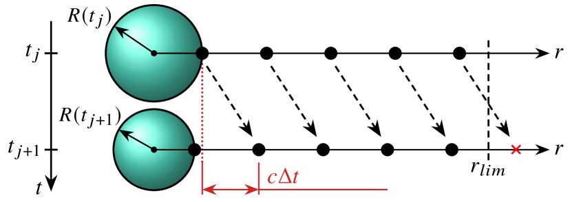
Following our previous work (Denner and Schenke, 2023a), the acoustic emissions of a cavitation bubble are tracked along outgoing characteristics with the speed of sound as emission nodes, as illustrated in Figure 1. Each emission node contains information about the radial location , the pressure and velocity fields and , and the invariants and of the acoustic emissions that follow from the employed model for the bubble dynamics. The radial coordinate of an emission node is updated at each time by
| (21) |
where is the number of time steps from to , and is the retarded time , representing the time at which the emission node is emitted at the bubble wall. The invariants and at the time of emission are readily obtained by evaluating Eq. (19) and Eq. (20) at as
| (22) | ||||
| (23) |
Inserting Eqs. (22) and (23) into Eqs. (19) and (20) then yields closed-form expressions for the local flow velocity and pressure (Denner and Schenke, 2023a) that satisfy the boundary condition at the bubble wall by reducing to and , respectively.
V Acoustic interactions
When the interaction of multiple bubbles is to be considered, the velocity and pressure contributions of all bubbles in a suitably sized neighborhood ought to be considered. Assuming a superposition of the potential in the liquid (Fuster and Colonius, 2011; Zhang et al., 2023), the local flow velocity and pressure at location in three-dimensional space are given as
| (24) | ||||
| (25) |
respectively, where is the number of bubbles and is the distance of the center of bubble to the location .
The driving pressure of each bubble is represented by the pressure in the liquid as if the considered bubble was absent, based on the ambient pressure , the acoustic excitation pressure (e.g., an ultrasound field), and the pressure contributed by the acoustic emissions of the neighbor bubbles. For bubble , the driving pressure is, therefore, defined as
| (26) |
with and where is the interaction pressure. The externally imposed acoustic excitation is either assumed to be spatially varying, representing a traveling wave, or spatially invariant, whereby all bubbles experience the same external acoustic excitation. The number of considered neighbor bubbles, , may include all bubbles of a population, as considered in this study, or only the bubbles in some predefined neighborhood of bubble . Additional details about the numerical computation of the interaction terms in Eq. (26) are given in Appendix A.
VI Results
To validate the proposed model for the dynamics and acoustic interactions of cavitation bubbles and bubble clusters, and to highlight the differences to previous work, we consider the frequency response of polydisperse microbubbles (Sec. VI.1), the resonance pattern of a bubble screen (Sec. VI.2), the asymmetric collapse of a spherical bubble cluster (Sec. VI.3), as well as the pressure-induced onset of cavitation in monodisperse and polydisperse bubble clusters (Sec. VI.4 and Sec. VI.5). The proposed methodology is implemented in the open-source software library APECSS (Denner and Schenke, 2023b), of which the version (v1.7) used to produce the presented results is available at https://doi.org/10.5281/zenodo.13850831.
VI.1 Frequency response of polydisperse microbubbles
Haghi, Sojahrood, and Kolios (2019) studied the resonance behavior of a small number interacting bubbles using a simplified Keller-Miksis equation,
| (28) |
where the second term on the right-hand side describes the bubble-bubble interactions. These interactions are assumed to be instantaneous, which is equivalent to assuming an incompressible liquid. They found that the dynamics of the smaller bubbles in a polydisperse cluster are strongly influenced by their neighbors of larger size, leading to two distinct scenarios:
-
1.
Constructive interactions, whereby the oscillations of smaller and larger bubbles are in phase, leading to amplified oscillations of the smaller bubbles.
-
2.
Destructive interactions, whereby the resonance modes of the smaller bubbles are suppressed and the oscillation dynamics of the smaller bubbles are governed by the larger bubbles in their neighborhood.
Because we want to compare the proposed quasi-acoustic model with the incompressible approach, we will use a more complete Keller-Miksis equation for our computations with the incompressible interaction term, defined for bubble as
| (29) |
where
| (30) |
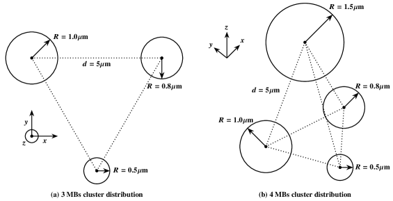
Following the work of Haghi, Sojahrood, and Kolios (2019), we consider the frequency response of two bubble clusters, schematically illustrated in Figure 2. The first cluster is composed of three bubbles with initial radii of , , and , located apart from each other on the corners of a regular triangle. The second cluster includes an additional bubble with a radius of , with the four bubbles located on the corners of a regular tetrahedron. The bubbles are assumed to contain air, with polytropic exponent , and are situated in water, with a density of , a speed of sound of , a dynamic viscosity of , and a surface tension coefficient of . The ambient pressure is . The bubble clusters are excited with a progressive sinusoidal wave defined as
| (31) |
with a pressure amplitude of , a frequency ranging from to , and where represents the -coordinate as illustrated in Figure 2. For each frequency, the maximum radius achieved by each bubble in periodic steady state is recorded.
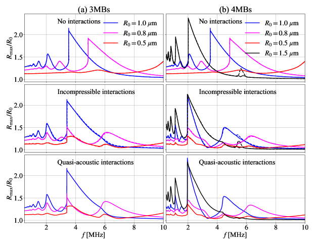
The maximum bubble radii as a function of the excitation frequency are shown in Figure 3, without bubble-bubble interactions (i.e., each bubble is considered as an isolated bubble), with incompressible bubble-bubble interactions (i.e., assuming the liquid speed of sound is infinite), and with quasi-acoustic bubble-bubble interactions (i.e., considering a finite liquid speed of sound). The results without interactions and with incompressible interactions are in excellent agreement with the results of Haghi, Sojahrood, and Kolios (2019). When acoustic interactions between the bubbles are considered, either incompressible or quasi-acoustic interactions, the largest bubble imposes its oscillation behavior onto the smaller bubbles, suppressing the resonance response of the smaller bubbles. However, the resulting differences between incompressible and quasi-acoustic interactions are small, which we attribute to the rather small separation distance of the bubbles of only , leading to nearly instantaneous interactions even when the finite propagation time of the acoustic emissions is considered with the proposed quasi-acoustic model.
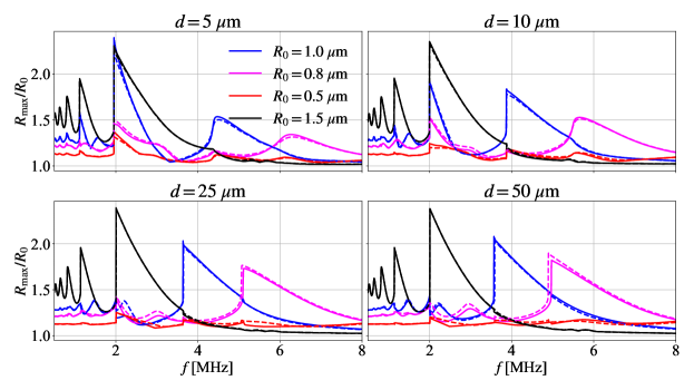
Figure 4 highlights the influence of the bubble-bubble distance. Increasing the distance separating the bubbles leads to less pronounced interactions, with a gradual recovery of the results obtained without considering interactions shown in Figure 3. An exception is the smaller bubble, which remains dominated by all its neighbors, not just the largest bubble. In addition, the differences in the bubble dynamics predicted with quasi-acoustic interactions compared to the incompressible interactions becomes more apparent when increasing the distance between the bubbles, especially for the smaller bubbles in the low-frequency range.
VI.2 Resonance patterns of a monodisperse bubble screen
Fan, Li, and Fuster (2021) studied the importance of accounting for the compressibility of the liquid and the associated finite propagation speed of acoustic waves for the bubble-bubble interaction. They demonstrated that the time delay of the bubble-bubble interactions in such clusters results in the formation of spatial patterns.
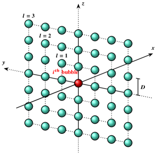
Following the work of Fan, Li, and Fuster (2021), we consider the bubble screen shown in Figure 5, consisting of 51 51 uniformly spaced bubbles that are excited by
| (32) |
where is the angular frequency. Each bubble has an initial radius of and the bubbles are located at a distance of . We consider an air-water system with a liquid density of , a speed of sound of , an ambient pressure of , an initial gas pressure of , and a polytropic exponent of the gas of . This choice of parameters leads to a Minneart resonance frequency (Minnaert, 1933) for each individual bubble of . The bubble screen is excited with an angular frequency of and a pressure amplitude of .
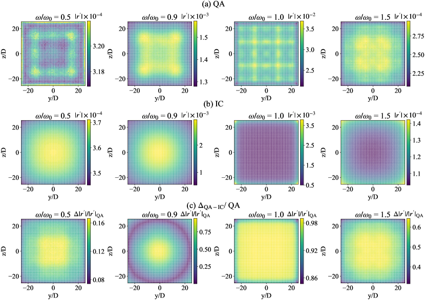
The dimensionless radial oscillation amplitude of each bubble in the bubble screen at periodic steady state is shown in Figure 6 for four excitation frequencies, with and representing respectively the maximum and minimum radius value during an oscillation period. The results obtained with the quasi-acoustic model are in good agreement with the results reported by Fan, Li, and Fuster (2021), especially with respect to the orders of magnitude of the oscillation amplitude. Qualitative differences in the amplitude pattern can be observed between our results and the results of Fan, Li, and Fuster (2021), which we attribute to differences in the chosen solution domain. While the proposed model solves the transient bubble dynamics and interactions in the time domain, Fan, Li, and Fuster (2021) solved the bubble dynamics and interactions in the frequency domain, thereby enforcing time periodicity.
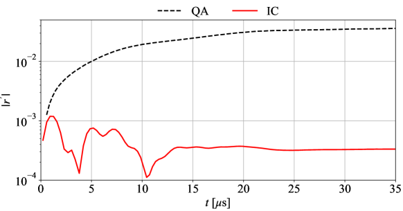
Considering instead incompressible bubble-bubble interactions, described by Eq. (29), the oscillations of the bubble screen show clear differences, see Figure 6, with respect to the magnitude of the oscillations and the amplitude patterns. For , the relative difference between the two models for the majority of the bubbles. This means that the radial oscillation amplitude for the incompressible model represents only 2 % of the value obtained with the quasi-acoustic model. This difference of approximately two orders of magnitude is also visible in Figure 7 for the center bubble. In addition, the bubbles require a longer time to reach a periodic steady state when considering quasi-acoustic interactions () as compared to when considering incompressible interactions (), see Figure 7.
VI.3 Asymmetric collapse of a spherical bubble cluster
When a traveling acoustic waves interacts with a bubble cluster, the response of the individual bubbles depends on their location (D’Agostino and Brennen, 1989; Wang and Brennen, 1999; Arora, Ohl, and Lohse, 2007); bubbles in the center are shielded by their neighbors, thus peripheral bubbles respond stronger to the acoustic excitation than inner bubbles. Using three-dimensional compressible flow simulations in which the bubbles are described using the Keller-Miksis model in conjunction with a Lagrangian particle tracking algorithm, Maeda and Colonius (2019) reproduced this behavior for a monodisperse spherical bubble cluster with 2500 bubbles.
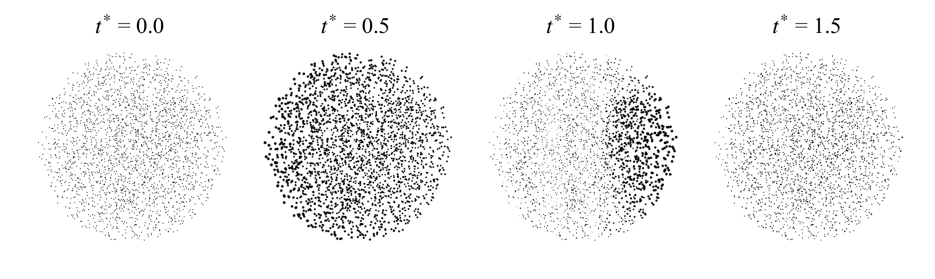
This test case involves a monodisperse spherical bubble cluster with a radius of , containing bubbles of initial radius . This cluster is excited by a single pulse of a sinusoidal wave propagating from left to right along the -axis,
| (33) |
with pressure amplitude and frequency , resulting in a wavelength () that is longer than . An air-water system is considered here, described by the same properties as presented in Section VI.1.
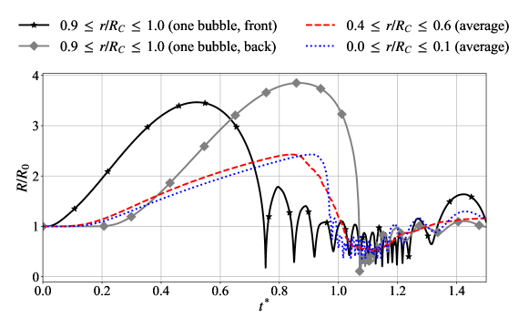
Figure 8 shows the bubble cluster at four distinct time instances. Qualitatively, the bubble cluster exhibits the same asymmetric expansion and collapse as previously observed in experiments (Arora, Ohl, and Lohse, 2007; Wang and Brennen, 1999) and three-dimensional compressible flow simulations (Maeda and Colonius, 2019). The evolution of the normalized bubble radius as a function of the dimensionless time in selected locations is shown in Figure 9. In agreement with previously reported results (Arora, Ohl, and Lohse, 2007; Maeda and Colonius, 2017), the bubbles near the edge of the cluster respond stronger to the passing excitation wave than the bubbles located near the center of the bubble cluster. This tendency is a consequence of the fact that bubbles near the edge of the bubble cluster have in general fewer immediate neighbors compared to the bubbles located in the interior of the bubble cluster, leading to fewer bubble-bubble interactions. In reality, the bubbles also disperse the incident wave and dissipate parts of its energy (Wang and Brennen, 1999; Ohl et al., 2024), further exacerbating the observed tendencies.
VI.4 Onset of cavitation of interacting bubbles
The onset of cavitation signified by an explosive expansion of preexisting bubbles in response to a sudden reduction in ambient pressure has previously been shown to be influenced significantly by bubble-bubble interactions (Ida, 2009; Fuster, Pham, and Zaleski, 2014). Similar to the behavior observed with respect to the frequency response of multi-bubble systems in Sec. VI.1, the behavior and response of larger bubbles dominate the behavior of smaller bubbles in their vicinity, which may delay the onset of cavitation of the smaller bubbles (Ida, 2009).
To study the onset of cavitation, the change in ambient pressure is defined, following the work of Ida (2009), as
| (34) |
with and being a desired negative pressure value. When neglecting the viscosity of the liquid, the liquid pressure at the bubble wall, Eq. (16), reduces to
| (35) |
Assuming the compression and expansion of the gas in the bubble is an isothermal process with , the critical pressure for the onset of cavitation of a single bubble can be computed by solving , leading to (Neppiras and Noltingk, 1951)
| (36) |
Following the work of Ida (2009), we consider the response of a two-bubble system to a reduction in pressure from to as described by Eq. (34). The two bubbles are located at a distance of from each other and have an initial radius of and , respectively. The system considered here is an air-water system, with a liquid density of , a speed of sound of , a liquid viscosity of and a polytropic exponent of the gas of . The surface tension coefficient is and the ambient pressure is . It is worth noting that Ida (2009) used a Rayleigh-Plesset equation with interaction terms treating the liquid as incompressible, given for bubble as
| (37) |
which does not account for the finite propagation speed of the emitted acoustic waves.
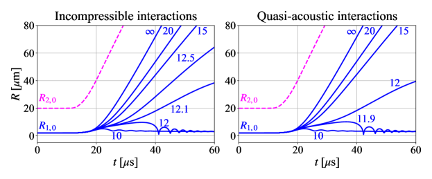
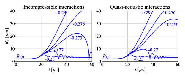
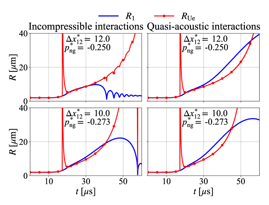
Based on Eq. (36), the critical pressure for the onset of cavitation of the two considered bubbles is and , respectively. As suggested by these critical pressure values, a negative pressure sufficient to promote the onset of cavitation of bubble 1 (the smaller bubble) is also sufficient to promote the onset of cavitation of bubble 2 (the larger bubble). Considering both incompressible and quasi-acoustic interactions, Figure 10 shows the radius evolution of both bubbles in response to a reduction in pressure to , for different separation distances of the bubbles, and Figure 11 shows the radius evolution of the smaller bubble (bubble 1) located at a distance of , for different negative pressure values . The results depicted in Figures 10 and 11 obtained with incompressible interactions are in very good agreement with the results reported by Ida (2009). It is noticeable that the onset of cavitation for the smaller bubble is observed at a smaller bubble-bubble distance, see Figure 10, and that the smaller bubble expands more under the same pressure conditions, see Figure 11, when considering quasi-acoustic interactions compared to incompressible interactions.
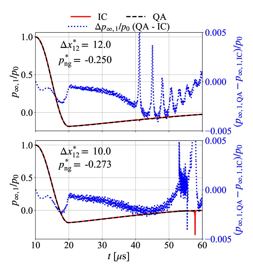
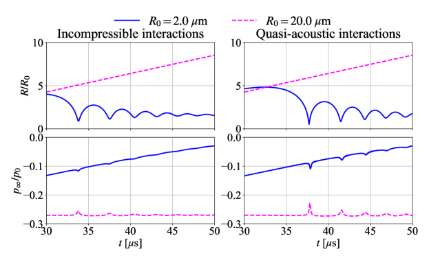
To better understand the differences between the two interaction models, the ambient pressure evolution for the smaller bubble is considered, as seen with Figure 12 for two different parameter pairs . After the pressure reduction defined by Eq. (34), the ambient pressure felt by the smaller bubble increases due to the pressure waves radiated by the larger bubble. During the expansion phase of the smaller bubble, , a consequence of the delayed interactions in the quasi-acoustic model.
For a bubble to continue expanding, it is necessary that ,(Ida, 2009) with denoting the unstable equilibrium radius. is obtained by solving
| (38) |
Because , is here the only real root of a third-order polynom. The smaller the ambient pressure, the smaller is the unstable radius. Because the ambient pressure is smaller when considering the quasi-acoustic model, it results in a smaller unstable radius, allowing the smaller bubble to expand more and for a longer time than in the case of incompressible interactions, see Figure 13.
Lastly, we consider the evolution of the ambient pressure during the collapse phase, see Figure 14. With both interaction models, during the collapse of the smaller bubble, the larger bubble sees an increase in its ambient pressure (dashed pink lines), while the smaller bubble experiences a pressure drop (solid blue lines). When collapsing, a bubble emits strong pressure waves that increase the ambient pressure felt by its neighbors for a short amount of time, hindering them in their expansion. This results in a smaller radiated pressure by the neighbor bubbles, explaining the ambient pressure drop experienced by the collapsing bubble. The stronger the collapse, the larger the pressure drop is, see the solid red curve in the bottom graph of Figure 12.
VI.5 Onset of cavitation of a spherical bubble cluster
To extend the test case presented in the previous section, we consider a spherical bubble cluster, similar to the cluster previously considered by Maeda and Colonius (2019) and in Section VI.3, which is subjected to a single tension pulse, defined as
| (39) |
where and is the duration of the pulse. The spherical bubble cluster has a radius of and consists of bubbles. Two initial radius distributions are considered: monodisperse bubbles with the initial radius and polydisperse bubbles with a log-normal size distribution. This log-normal distribution is defined by , where is the reference bubble size, is the mean and is the standard deviation of the distribution, with the values of and adopted from previous work (Ando, Colonius, and Brennen, 2011; Maeda and Colonius, 2019). We again assume an air-water system, with the same fluid properties as used in Section VI.1. This choice of parameters leads to a critical pressure for the onset of cavitation of with respect to a single bubble. Both bubble clusters are subject to a tension wave described by Eq. (39), with and . With this duration , the pressure pulse has a wavelength of , such that the assumption that the pulse is dependent on time but not space, see Eq. (39), is justified.
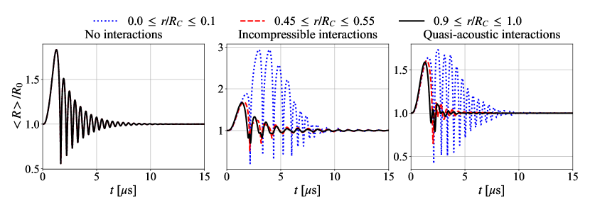
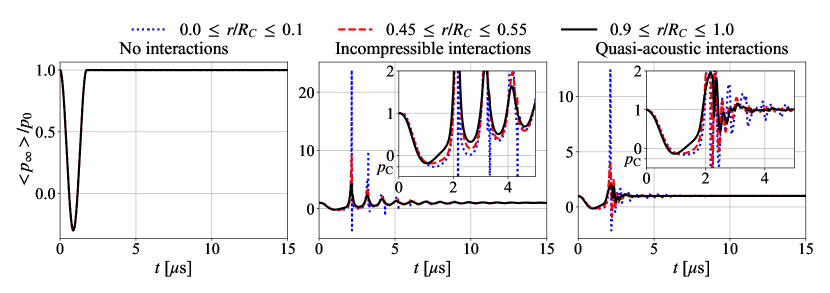
The results for the monodisperse cluster are shown in Figures 15 and 16, obtained with incompressible and quasi-acoustic interactions, as well as by neglecting interactions between the bubbles. When the interactions between the bubble are neglected, every bubble in the cluster experiences the same pressure, leading to the same radius evolution. Interestingly, with both interaction models, the response to the pulse of the bubbles near the cluster center is most pronounced. Since the considered tension pulse is only dependent on time but not space, the asymmetric collapse tendency highlighted by Wang and Brennen (1999) or Nasibullaeva and Akhatov (2013), and also observed in Section VI.3, is not present here. In the present case, the number of close neighbors is the key factor influencing the response of a bubble. Near the edge of the bubble cluster, the tension pulse is the dominant excitation experienced by the bubbles since they have few close neighbors. Closer to the center of the bubble cluster, the number of neighbors for each bubble increases, and the pressure emitted by these neighbors becomes an additional excitation for these bubbles. As seen in Figure 16, the magnitude of the normalized mean pressure experienced by the bubbles in a specific region of the bubble cluster is highest near the center of the cluster. The incompressible interactions yield larger amplitudes of the radius and pressure oscillations than the quasi-acoustic interactions. In fact, when neglecting the propagation time of the emission, the pressure changes induced by the interactions are felt at the same time for each bubble in the cluster, resulting in pressure peaks that are larger and more concentrated in time. The incompressible interactions also maintain the excitation state initiated by the incident pulse for a longer time, due to the larger and faster initial pressure increase. Indeed, this first pressure peak is followed by two smaller peaks, as seen in the center graph of Figure 16. Such secondary pressure peaks are not observed when considering quasi-acoustic interactions, see the right graph of Figure 16, explaining the faster recovery of the undisturbed state.
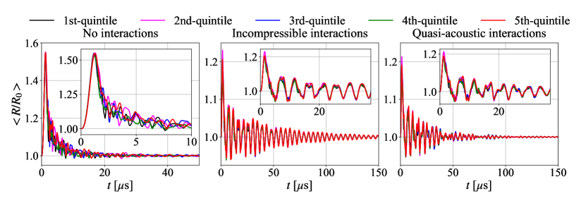
The results of the polydisperse cluster are presented in Figure 17, showing the dimensionless mean radius based on a quintile repartition of the initial radius distribution. Neglecting the interactions between the bubbles, small discrepancies between the dynamics of each bubble group are noticeable. However these differences in behavior disappear when taking bubble-bubble interactions into account. This tendency is consistent with previous numerical observations reported by Nasibullaeva and Akhatov (2013), where in a polydisperse cluster with two initial bubble radii groups, both bubble groups synchronize their oscillations, similar to what is seen in the Figure 17. Also, each bubble attains a smaller maximum radius when bubble-bubble interactions are taken into account, as a results of the acoustic emissions of their neighbors. The main difference in this case is between the two interaction models: when considering quasi-acoustic interactions, the system is more damped compared to when incompressible interactions are considered, with a faster decay of the oscillation amplitude for each bubble group. Like stated with the monodisperse cluster, the delayed interactions maintain for a shorter time the excited state induced by the incident pulse.
VII Conclusions
We have presented a new model for the bubble dynamics, acoustic emissions and interactions based on the quasi-acoustic assumption and in spherical symmetry. This model builds on the Keller-Miksis equation for the radial bubble dynamics and a Lagrangian wave tracking approach of the acoustic emissions and interactions of the bubbles, and takes the compressibility of the liquid surrounding the bubbles consistently into account up to first order in the Mach number.
Representative and well-defined test-cases, including monodisperse and polydisperse bubble clusters, have been used to validate the proposed model and highlight the differences compared to the commonly used class of models derived under the assumption of an incompressible liquid. The presented results show excellent agreement with previously reported phenomena of multi-bubble systems, such as the dominance of larger bubbles on the resonance behavior of smaller bubbles, the asymmetric collapse of bubble clusters, and the delayed onset of cavitation of smaller bubbles in the vicinity of larger bubbles. Contrary to the widely used models based on incompressible interactions, accounting for the finite propagation speed of the acoustic emissions, has been found to affect the oscillation patterns in bubble screens, the onset of cavitation of multi-bubble systems, as well as the response of bubble clusters to tension waves. The differences between models based on incompressible interactions and the proposed quasi-acoustic model are most pronounced for large and dense bubble systems, in which the finite propagation speed and the resulting time delay of the acoustic interactions becomes appreciable and results in markedly different bubble dynamics.
In deriving and testing the proposed model based on the quasi-acoustic assumption, we have neglected the translational motion of the bubbles, for instance as a result of secondary Bjerknes forces associated with the acoustic interaction of the bubbles. However, because the proposed quasi-acoustic model readily provides the flow velocity and pressure associated with the acoustic emissions of the bubbles, see Eqs. (24) and (25), combining the proposed model with a methodology to track the motion of the bubbles would be straightforward. Additionally, the use of the Keller-Miksis equation limits this model to cases with moderate pressure amplitudes such that the density and the speed of sound remain approximately constant. For water, this assumption yields errors with respect to the density and speed of sound that are smaller than for pressures up to compared to ambient conditions, according to the IAPWS R6-95(2018) standard (Wagner and Pruß, 2002).
In summary, the proposed model provides a consistent computational tool to simulate the radial dynamics, acoustic emissions and interactions of multi-bubble systems, enabling a more faithful prediction of the acoustic emissions and interactions than the frequently employed incompressible models, with a reduced complexity and faster execution compared to state-of-the-art CFD methods.
Acknowledgements
We acknowledge the support of the Natural Sciences and Engineering Research Council of Canada (NSERC), funding reference number RGPIN-2024-04805, as well as fruitful discussions with Yuzhe Fan, Daniel Fuster, Hossein Haghi and Sören Schenke on acoustic bubble-bubble interactions and the numerical modeling of cavitation.
Data availability
Data supporting this study is available at https://doi.org/10.5281/zenodo.13891010 under a Creative Commons Attribution license.
Appendix A Computing the interaction terms
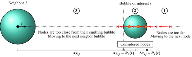
The quasi-acoustic interactions are modeled using the Lagrangian wave tracking previously proposed by Denner and Schenke (2023a). The information carried by the Lagrangian wave tracking allows to compute the interaction terms given in Eq. (26) for the neighbor bubbles. For each bubble, and are obtained from their neighbor bubbles at predefined time intervals by employing the following strategy, illustrated in Figure 18. Considering the bubble of interest and its neighbor , we commence by parsing the list of emission nodes of bubble , starting with the emission node that is furthest away from its bubble . When all emission nodes of bubble that are located inside bubble are identified, we stop parsing the list of emission nodes of bubble . The mean values of the invariants and of all emission nodes of bubble located inside bubble are then used to compute the interaction pressure in Eq. (26). Other ways of determining and may also be considered, such as weighting the contribution of the emission nodes by a Gaussian or a radial basis function with finite support. The time derivative of the resulting interaction pressure, which is part of the pressure derivative in Eq. (27), is computed numerically as
| (40) |
To reduce the computational cost for large bubble clusters, we prune emission nodes that do not carry relevant information. Based on Eq. (20), an emission node is considered to be obsolete if its pressure amplitude is
| (41) |
The rationale behind this condition is that emission nodes make a significant contribution to the interactions only if the global pressure considering every node is relevant in comparison to . Since at the moment we consider every bubble to be interacting with all bubbles of a cluster, is divided by the total number of bubbles . The coefficient is a case-dependent coefficient that has so far been determined mainly by trial and error, with the goal of reducing the execution time without neglecting the main pressure changes induced by the interactions and thereby compromising the results.
References
- Matsumoto and Yoshizawa (2005) Y. Matsumoto and S. Yoshizawa, “Behaviour of a bubble cluster in an ultrasound field,” International Journal for Numerical Methods in Fluids 47, 591–601 (2005).
- Song, Moldovan, and Prentice (2019) J. H. Song, A. Moldovan, and P. Prentice, “Non-linear Acoustic Emissions from Therapeutically Driven Contrast Agent Microbubbles,” Ultrasound in Medicine & Biology 45, 2188–2204 (2019).
- Franc and Michel (2005) J.-P. Franc and J.-M. Michel, Fundamentals of Cavitation, Fluid Mechanics and Its Applications, Vol. 76 (Kluwer Academic Publishers, Dordrecht, 2005).
- Hsiao and Chahine (2015) C.-T. Hsiao and G. L. Chahine, “Dynamic response of a composite propeller blade subjected to shock and bubble pressure loading,” Journal of Fluids and Structures 54, 760–783 (2015).
- Dular et al. (2019) M. Dular, T. Požar, J. Zevnik, and R. Petkovšek, “High speed observation of damage created by a collapse of a single cavitation bubble,” Wear 418-419, 13–23 (2019).
- Salzar et al. (2017) R. S. Salzar, D. Treichler, A. Wardlaw, G. Weiss, and J. Goeller, “Experimental Investigation of Cavitation as a Possible Damage Mechanism in Blast-Induced Traumatic Brain Injury in Post-Mortem Human Subject Heads,” Journal of Neurotrauma 34, 1589–1602 (2017).
- Walls et al. (2017) P. L. L. Walls, O. McRae, V. Natarajan, C. Johnson, C. Antoniou, and J. C. Bird, “Quantifying the potential for bursting bubbles to damage suspended cells,” Scientific Reports 7, 15102 (2017).
- Johnsen and Colonius (2009) E. Johnsen and T. Colonius, “Numerical simulations of non-spherical bubble collapse,” Journal of Fluid Mechanics 629, 231–262 (2009).
- Ida (2009) M. Ida, “Multibubble cavitation inception,” Physics of Fluids 21, 113302 (2009).
- Wang and Brennen (1999) Y.-C. Wang and C. E. Brennen, “Numerical Computation of Shock Waves in a Spherical Cloud of Cavitation Bubbles,” Journal of Fluids Engineering 121, 872–880 (1999).
- Shen et al. (2021) Y. Shen, L. Zhang, Y. Wu, and W. Chen, “The role of the bubble–bubble interaction on radial pulsations of bubbles,” Ultrasonics Sonochemistry 73, 105535 (2021).
- Deng et al. (2024) F. Deng, D. Zhao, L. Zhang, and Y. Li, “Acoustic radiation of bubble clusters with different volume fractions,” Physics of Fluids 36, 033308 (2024).
- Rayleigh (1917) L. Rayleigh, “On the pressure developed in a liquid during the collapse of a spherical cavity,” Philosophical Magazine 34, 94–98 (1917).
- Gilmore (1952) F. R. Gilmore, “The growth or collapse of a spherical bubble in a viscous compressible liquid,” Tech. Rep. Report No. 26-4 (California Institute of Technology, Pasadena, California, USA, 1952).
- Trilling (1952) L. Trilling, “The Collapse and Rebound of a Gas Bubble,” Journal of Applied Physics 23, 14–17 (1952).
- Keller and Miksis (1980) J. B. Keller and M. Miksis, “Bubble oscillations of large amplitude,” The Journal of the Acoustical Society of America 68, 628–633 (1980).
- Prosperetti and Lezzi (1986) A. Prosperetti and A. Lezzi, “Bubble dynamics in a compressible liquid. Part 1. First-order theory,” Journal of Fluid Mechanics 168, 457–478 (1986).
- Lezzi and Prosperetti (1987) A. Lezzi and A. Prosperetti, “Bubble dynamics in a compressible liquid. Part 2. Second-order theory,” Journal of Fluid Mechanics 185, 289–321 (1987).
- Denner (2021) F. Denner, “The Gilmore-NASG model to predict single-bubble cavitation in compressible liquids,” Ultrasonics Sonochemistry 70, 105307 (2021).
- Fuster, Conoir, and Colonius (2014) D. Fuster, J. M. Conoir, and T. Colonius, “Effect of direct bubble-bubble interactions on linear-wave propagation in bubbly liquids,” Physical Review E 90, 063010 (2014).
- Fuster (2019) D. Fuster, “A Review of Models for Bubble Clusters in Cavitating Flows,” Flow, Turbulence and Combustion 102, 497–536 (2019).
- Plesset and Prosperetti (1977) M. S. Plesset and A. Prosperetti, “Bubble Dynamics and Cavitation,” Annual Review of Fluid Mechanics 9, 145–185 (1977).
- Lauterborn and Kurz (2010) W. Lauterborn and T. Kurz, “Physics of bubble oscillations,” Reports on Progress in Physics 73, 106501 (2010).
- Denner (2024) F. Denner, “The Kirkwood–Bethe hypothesis for bubble dynamics, cavitation, and underwater explosions,” Physics of Fluids 36, 051302 (2024).
- Fu et al. (2023) L. Fu, X.-X. Liang, S. Wang, S. Wang, P. Wang, Z. Zhang, J. Wang, A. Vogel, and C. Yao, “Laser induced spherical bubble dynamics in partially confined geometry with acoustic feedback from container walls,” Ultrasonics Sonochemistry 101, 106664 (2023).
- Stricker, Prosperetti, and Lohse (2011) L. Stricker, A. Prosperetti, and D. Lohse, “Validation of an approximate model for the thermal behavior in acoustically driven bubbles,” The Journal of the Acoustical Society of America 130, 3243–3251 (2011).
- Zhou and Prosperetti (2020) G. Zhou and A. Prosperetti, “Modelling the thermal behaviour of gas bubbles,” Journal of Fluid Mechanics 901, R3 (2020).
- Klapcsik and Hegedűs (2019) K. Klapcsik and F. Hegedűs, “Study of non-spherical bubble oscillations under acoustic irradiation in viscous liquid,” Ultrasonics Sonochemistry 54, 256–273 (2019).
- Folden and Aschmoneit (2023) T. S. Folden and F. J. Aschmoneit, “A classification and review of cavitation models with an emphasis on physical aspects of cavitation,” Physics of Fluids 35, 081301 (2023).
- Mnich et al. (2024) D. Mnich, F. Reuter, F. Denner, and C.-D. Ohl, “Single cavitation bubble dynamics in a stagnation flow,” Journal of Fluid Mechanics 979, A18 (2024).
- Saini et al. (2024) M. Saini, Y. Saade, D. Fuster, and D. Lohse, “Finite speed of sound effects on asymmetry in multibubble cavitation,” Physical Review Fluids 9, 043602 (2024).
- Fan, Li, and Fuster (2021) Y. Fan, H. Li, and D. Fuster, “Time-delayed interactions on acoustically driven bubbly screens,” The Journal of the Acoustical Society of America 150, 4219–4231 (2021).
- Haghi and Kolios (2022) H. Haghi and M. C. Kolios, “The role of primary and secondary delays in the effective resonance frequency of acoustically interacting microbubbles,” Ultrasonics Sonochemistry 86, 106033 (2022).
- Mettin et al. (1997) R. Mettin, I. Akhatov, U. Parlitz, C.-D. Ohl, and W. Lauterborn, “Bjerknes forces between small cavitation bubbles in a strong acoustic field,” Physical Review E 56, 2924–2931 (1997).
- Jiang et al. (2012) L. Jiang, F. Liu, H. Chen, J. Wang, and D. Chen, “Frequency spectrum of the noise emitted by two interacting cavitation bubbles in strong acoustic fields,” Physical Review E 85, 036312 (2012).
- Jiang et al. (2017) L. Jiang, H. Ge, F. Liu, and D. Chen, “Investigations on dynamics of interacting cavitation bubbles in strong acoustic fields,” Ultrasonics Sonochemistry 34, 90–97 (2017).
- Haghi, Sojahrood, and Kolios (2019) H. Haghi, A. Sojahrood, and M. C. Kolios, “Collective nonlinear behavior of interacting polydisperse microbubble clusters,” Ultrasonics Sonochemistry 58, 104708 (2019).
- Guédra, Cornu, and Inserra (2017) M. Guédra, C. Cornu, and C. Inserra, “A derivation of the stable cavitation threshold accounting for bubble-bubble interactions,” Ultrasonics Sonochemistry 38, 168–173 (2017).
- Yasui et al. (2009) K. Yasui, J. Lee, T. Tuziuti, A. Towata, T. Kozuka, and Y. Iida, “Influence of the bubble-bubble interaction on destruction of encapsulated microbubbles under ultrasound,” The Journal of the Acoustical Society of America 126, 973–982 (2009).
- D’Agostino and Brennen (1989) L. D’Agostino and C. E. Brennen, “Linearized dynamics of spherical bubble clouds,” Journal of Fluid Mechanics 199, 155–176 (1989).
- Arora, Ohl, and Lohse (2007) M. Arora, C. D. Ohl, and D. Lohse, “Effect of nuclei concentration on cavitation cluster dynamics,” The Journal of the Acoustical Society of America 121, 3432–3436 (2007).
- Nasibullaeva and Akhatov (2013) E. S. Nasibullaeva and I. S. Akhatov, “Bubble cluster dynamics in an acoustic field,” The Journal of the Acoustical Society of America 133, 3727–3738 (2013).
- Zhao et al. (2020) G. Zhao, W. Chen, F. Tao, L. Zhang, and Y. Wu, “Dynamics of bubbles in cavitation cloud based on lattice model,” Journal of Applied Physics 127, 244701 (2020).
- Ohl et al. (2024) S.-W. Ohl, J. M. Rosselló, D. Fuster, and C.-D. Ohl, “Finite amplitude wave propagation through bubbly fluids,” International Journal of Multiphase Flow 176, 104826 (2024).
- Bremond et al. (2006) N. Bremond, M. Arora, C.-D. Ohl, and D. Lohse, “Controlled Multibubble Surface Cavitation,” Physical Review Letters 96, 224501 (2006).
- Minnaert (1933) M. Minnaert, “XVI. On musical air-bubbles and the sounds of running water,” The London, Edinburgh, and Dublin Philosophical Magazine and Journal of Science 16, 235–248 (1933).
- Prosperetti (1984) A. Prosperetti, “Bubble phenomena in sound fields: part one,” Ultrasonics 22, 69–77 (1984).
- Denner and Schenke (2023a) F. Denner and S. Schenke, “Modeling acoustic emissions and shock formation of cavitation bubbles,” Physics of Fluids 35, 012114 (2023a).
- Fuster and Colonius (2011) D. Fuster and T. Colonius, “Modelling bubble clusters in compressible liquids,” Journal of Fluid Mechanics 688, 352–389 (2011).
- Zhang et al. (2023) A.-M. Zhang, S.-M. Li, P. Cui, S. Li, and Y.-L. Liu, “A unified theory for bubble dynamics,” Physics of Fluids 35, 033323 (2023).
- Denner and Schenke (2023b) F. Denner and S. Schenke, “APECSS: A software library for cavitation bubble dynamics and acoustic emissions,” Journal of Open Source Software 8, 5435 (2023b).
- Maeda and Colonius (2019) K. Maeda and T. Colonius, “Bubble cloud dynamics in an ultrasound field,” Journal of Fluid Mechanics 862, 1105–1134 (2019).
- Maeda and Colonius (2017) K. Maeda and T. Colonius, “A source term approach for generation of one-way acoustic waves in the Euler and Navier–Stokes equations,” Wave Motion 75, 36–49 (2017).
- Fuster, Pham, and Zaleski (2014) D. Fuster, K. Pham, and S. Zaleski, “Stability of bubbly liquids and its connection to the process of cavitation inception,” Physics of Fluids 26, 042002 (2014).
- Neppiras and Noltingk (1951) E. A. Neppiras and B. E. Noltingk, “Cavitation Produced by Ultrasonics: Theoretical Conditions for the Onset of Cavitation,” Proceedings of the Physical Society. Section B 64, 1032–1038 (1951).
- Ando, Colonius, and Brennen (2011) K. Ando, T. Colonius, and C. E. Brennen, “Numerical simulation of shock propagation in a polydisperse bubbly liquid,” International Journal of Multiphase Flow 37, 596–608 (2011).
- Wagner and Pruß (2002) W. Wagner and A. Pruß, “The IAPWS Formulation 1995 for the Thermodynamic Properties of Ordinary Water Substance for General and Scientific Use,” Journal of Physical and Chemical Reference Data 31, 387–535 (2002).