Massive Fields Affected by Echoes: New Physics vs. Astrophysical Environment
Abstract
Unlike the perturbations of massless fields, the asymptotic tails of massive fields exhibit oscillations and decay slowly, following a power-law envelope. In this work, considering various scenarios admitting (either fundamental or effective) massive scalar and gravitational fields, we demonstrate that bump deformations in the effective potential, either in the near-horizon or far-field regions, modify these asymptotic oscillatory tails. Specifically, the power-law envelope transitions to a more complex oscillatory pattern, which cannot be easily fitted to a simple formula. This behavior is qualitatively different from the echoes of massless fields, which appear mainly during the quasinormal ringing stage and are considerably suppressed at the asymptotic tails. We show that in some models echoes may considerably amplify the signal at the stage of asymptotic tails.
pacs:
04.30.-w,04.50.Kd,04.70.BwI Introduction
Echoes are modifications of a signal at late times stipulated by the secondary scatterings of the wave from additional maxima of the effective potential Cardoso et al. (2016a); Cardoso and Pani (2017); Barausse et al. (2014). While echoes of massless fields have been studied in a great number publications (see, for instance, Cardoso et al. (2016a); Cardoso and Pani (2017); Barausse et al. (2014); Huang et al. (2022); Konoplya et al. (2019); Abedi et al. (2017); Mark et al. (2017); Wang et al. (2020); Bronnikov and Konoplya (2020); Bueno et al. (2018); Churilova et al. (2021); Guo et al. (2022); Churilova and Stuchlik (2020); Li and Piao (2019); Buoninfante (2020); Liu et al. (2021); Chowdhury et al. (2022); Yang et al. (2024a); Shen et al. (2024); Yang et al. (2024b) and references therein), echoes in the massive gravity, to the best of our knowledge, were discussed only in Dong and Stojkovic (2021) where no effects for effectively massive fields were reported. However, the time-domain profiles for the Kaluza-Klein gravitational degrees of freedom in the braneworld scenario have been recently obtained in Tan et al. (2024).
At the same time, there are several motivations to study the evolution of perturbations in massive fields. Firstly, fields that are initially massless may acquire an effective mass term due to the influence of tidal forces in brane-world models and other extra-dimensional scenarios Seahra et al. (2005); Ishihara et al. (2008), or in the presence of a magnetic field Konoplya and Fontana (2008); Konoplya (2008); Wu and Xu (2015). Additionally, massive gravitons and other massive particles are expected to contribute to long-wavelength gravitational waves Konoplya and Zhidenko (2024a), which are currently being investigated through Pulsar Timing Array observations Afzal et al. (2023).
The quasinormal modes of massive fields differ qualitatively from those of massless fields, particularly due to the strong suppression of the damping rate. In some cases, this leads to the existence of arbitrarily long-lived modes, known as quasi-resonances, within the spectrum Ohashi and Sakagami (2004); Konoplya and Zhidenko (2005, 2006); Zhidenko (2006). Moreover, the asymptotic tails of massive fields exhibit distinct behavior, as they do not decay according to the power-law characteristic of massless fields. Instead, they oscillate and decay slowly with a power-law envelope (see the review in Konoplya and Zhidenko (2011)).
In this work, we address a gap in the literature by studying echoes in massive fields. To this end, we consider three different models: the simplest massive scalar field in a Schwarzschild background, the squashed Kaluza-Klein black hole, and a wormhole mimicking the Schwarzschild solution Damour and Solodukhin (2007). In the first two models, echoes are induced by a deformation in the effective potential, creating a bump. In contrast, the third model features a double-well potential, producing echoes without the need for an additional bump.
We have demonstrated that echoes in massive fields are markedly different from those in massless fields. Specifically, when the bump is localised in the far zone, they affect the signal more during the asymptotic tail stage, leading to the oscillation of the power law envelope. The near-horizon bumps, one the contrary, induce the distinctive echoes effects in some cases at the earlier stage of quasinormal ringing. Given the slow decay of the asymptotic tails in massive fields, this enhances the significance of echoes in such fields.
The paper is organized as follows. In Section II, we examine the echoes of a massive scalar field in a Schwarzschild background, focusing on cases where the effective potential has a bump both at a distance and near the horizon. In Section III, we analyze the echoes of gravitational perturbations (effectively massive) around squashed Kaluza-Klein black holes. Section IV is dedicated to the study of echoes of massive fields around the Schwarzschild-like wormhole.
II Schwarzschild black hole with the Gaussian bump in the effective potential
The simplest model for the decay of a massive field in a black hole background involves a minimally coupled massive scalar field in the Schwarzschild background. Echoes are then produced by a deformation in the effective potential’s bump. A more self-consistent approach would require the deformation of the mass function to incorporate an appropriate bump. However, when the bump is either small or located far from the black hole, its back-reaction on the background metric can be safely neglected.
We consider the Schwarzschild black hole, which is given by the following line element
| (1) |
where
and is the radius of the event horizon.
The Klein-Gordon equation for a massive scalar field
| (2) |
after separation of the angular part
can be reduced to the wavelike form
| (3) |
Here is the tortoise coordinate,
and the effective potential is given by
| (4) |
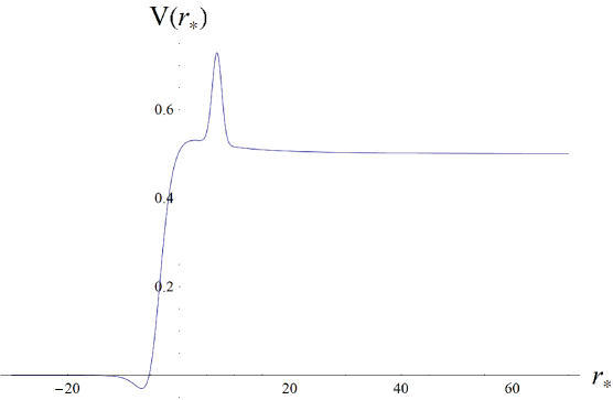
We add a bump to the effective potential
| (5) |
where
| (6) |
Here is the bump size, is the point of its maximum and is the width parameter.
To study the time-domain evolution of perturbations in these black hole models, we use the well-known time-domain integration scheme proposed in Gundlach et al. (1994). We apply the discretization scheme in terms of the light-cone variables and ,
where we used the following notation for the points: , , , and . This discretization scheme has been widely applied in numerous studies (see Konoplya (2024); Dubinsky and Zinhailo (2024); Dubinsky (2024); Konoplya and Zinhailo (2020); Skvortsova (2024); Bolokhov (2024a, b); Malik (2024a, b); Konoplya and Stashko (2024) for recent examples). The Gaussian initial data are imposed on the two null surfaces, and :
| (8) |
so that the positive value of the parameter corresponds to the Gaussian peak on the “west” null surface with respect to the observer, i.e., between the observer and the event horizon. The observer’s position is fixed at , which corresponds to the radial coordinate .
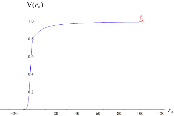
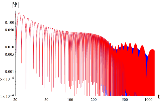
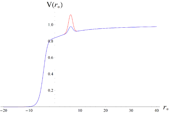
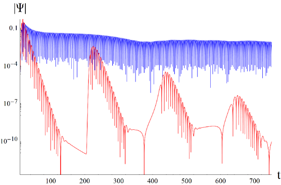
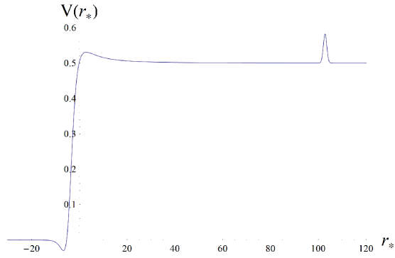
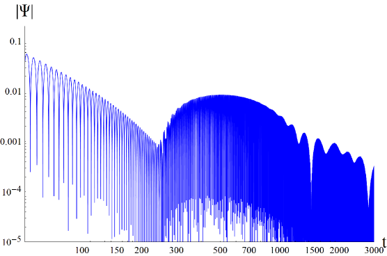
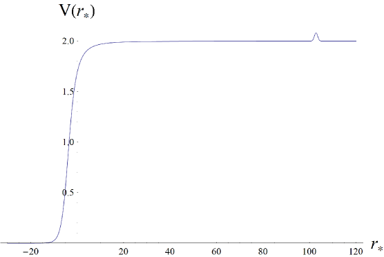
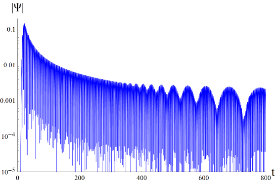
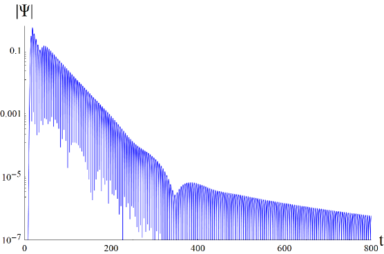
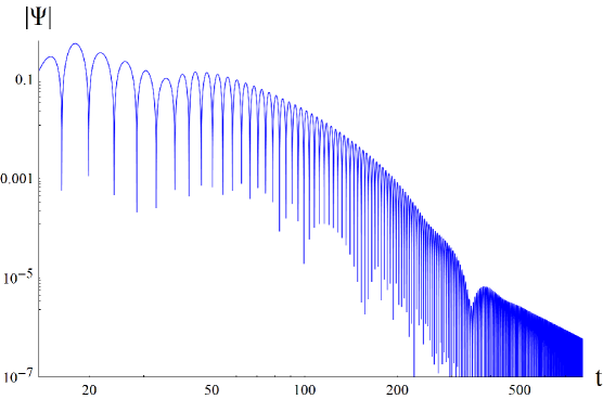
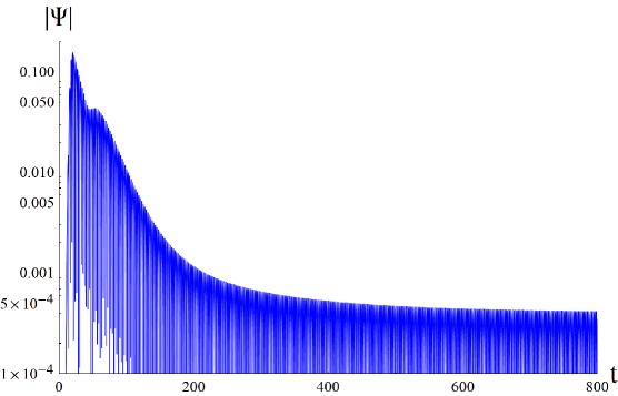
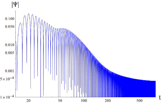
We can observe how the perturbations evolve over time, depending on various parameters such as the bump characteristics, the field’s mass, and the observer’s position. From the plot 1 one can see that, when the bump is located far from the black hole, echoes appear at very late times, modifying the power-law tail envelope, which becomes oscillatory with a non-constant period and amplitude. For smaller bumps, the amplitude of the oscillations decreases, and the farther the bump is from the black hole, the later the echoes appear. When the bump is closer to the event horizon, as shown in Fig. 2, both the intermediate tails and the final stage of the ringing phase are significantly modified. However, the asymptotic late-time tails, being governed by the asymptotic behavior of the potential, change insignificantly. Therefore, in order to observe the distinct echoes for the massive field, we need a significant modification of the effective potential outside the radiation zone. Such a modification can appear at a distance, due to another compact object with a comparable mass, e.g., a black hole or a neutron star, or, alternatively, due to the effects of new physics near the horizon or instead of the horizon. The latter effect for a Schwarzschild wormhole we shall consider in Sec. IV.
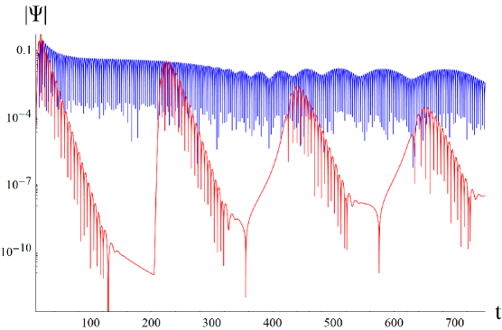
For sufficiently small bumps near the event horizon, the time-domain profile during the ringdown phase does not differ significantly from that of the spacetime without a bump. This result aligns with Konoplya and Zhidenko (2024b); Konoplya (2023), where it was demonstrated that the fundamental mode typically changes only slightly when the potential is slightly deformed near the horizon, with stronger deviations seen in the first few overtones. These overtones decay quickly, and for massive fields, their contribution to the time-domain profile is suppressed because (a) the fundamental mode decays more slowly and (b) the tails of massive fields begin to dominate earlier, leaving a relatively short period for the ringing phase.
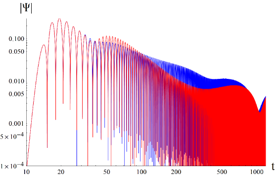
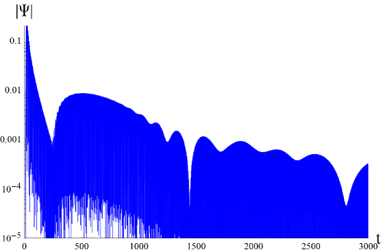
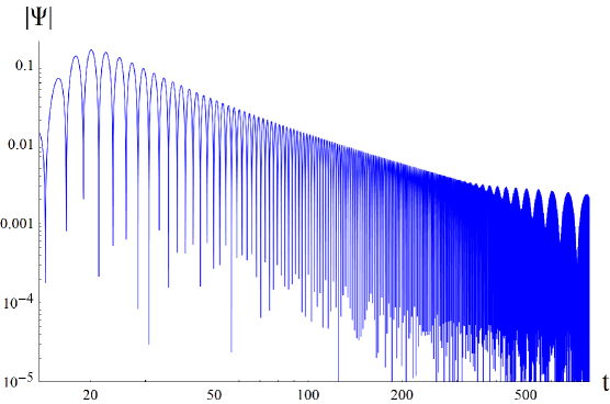
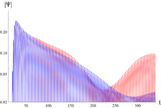
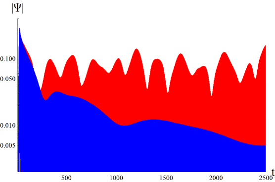
When comparing the echoes for massive and massless fields (see Fig. 3), we observe that the massless field, being long ranged, scatters the energy faster and, therefore the amplitude of echoes are many orders smaller. Even for an unrealistically, for astrophysical environment, large bump () we see that, although the amplitude of the first echo is of the same order of magnitude as the intermediate time tail, each next echo’s amplitude becomes by orders smaller than the echo for the massive field.
III Gravitational perturbations of squashed black holes in the Kaluza-Klein theory
Squashed Kaluza-Klein (KK) black holes Ishihara and Matsuno (2006) exhibit significant differences from standard Schwarzschild black holes, which are characterized by asymptotic flatness, and from black strings, even at energy levels where KK modes have not yet been activated. This makes squashed KK black holes a valuable model for exploring the dynamics of higher-dimensional spacetimes. Unlike their more conventional counterparts, these squashed black holes offer unique insights into higher dimensions, providing a glimpse into physics beyond the familiar four-dimensional framework.
One particularly noteworthy aspect of squashed KK black holes is their apparent stability Ishihara et al. (2008). This distinguishes them from other higher-dimensional solutions, such as black strings, which are prone to the Gregory-Laflamme instability Gregory and Laflamme (1993)—a phenomenon that can cause certain configurations to become dynamically unstable and fragment. The inherent stability of squashed KK black holes allows us to bypass this instability, making them more viable candidates.
The metric of the uncharged non-rotating squashed Kaluza-Klein black hole is Ishihara et al. (2008)
where is the angular coordinate, and we employ the following angular basis:
| (10) | |||||
and
Here is the radius of the event horizon and defines the compact coordinate scale,
so that corresponds to the non-Kaluza-Klein (Schwarzschild) black hole.
As shown in Kimura et al. (2008), the linearized perturbation equations of the gravitational field for zero modes with respect to the group are also reduced to the wave-like form with the following effective potentials,
Here are the eigenvalues corresponding to the group. is the massless degree of freedom of the gravitational perturbations while and gain an effective mass.
From Figures 4 and 5, we observe that, similar to the case of massive scalar field perturbations, when the bump is located at a considerable distance from the black hole, the echoes start to modify the power-law behavior of the asymptotic tails, turning them into an oscillatory pattern. As the bump moves closer to the event horizon, the echoes appear earlier and begin to influence the ringing phase. Similar to the case of the Schwarzschild black hole, to observe echoes, the geometry needs to be modified at a distance from the radiation zone (Fig. 4). A potential bump of the same size affects the perturbation profile more significantly due to the smaller effective mass.
IV Schwarzschild-like wormholes
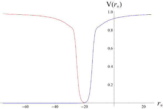
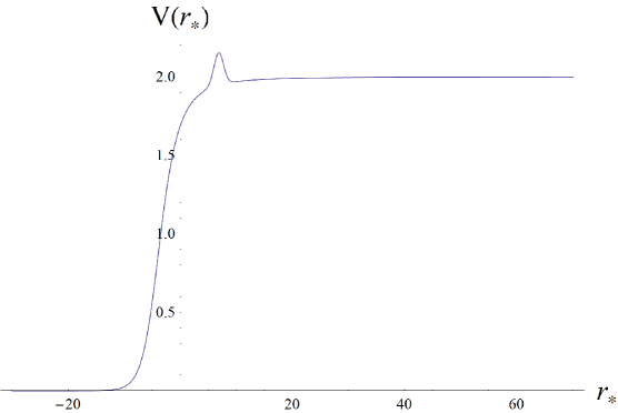
In this work, we consider -symmetric Schwarzschild-like wormholes Cardoso et al. (2016b) by assuming a Schwarzschild spacetime everywhere except at the wormhole throat, where a thin shell of matter is placed. The throat is positioned near the event horizon, at and we examine the region on both sides of the throat. For massless fields, the effective potential in this configuration takes the form of a double-peak potential, where the single peak in the Schwarzschild spacetime is split into two due to the symmetry of the radial coordinate. The echoes in this case arise from secondary scattering and reflection between the two peaks.
However, when a relatively large mass term is introduced, the potential shifts to a single-well form, approaching at both spatial infinities (see Figure 6). This modification results in distinct behavior in both the ringing phase and the asymptotic tails, while leaving the early stages of the ringing phase largely unaffected. The most notable effect is a significant amplification of the asymptotic tails, which reach a similar magnitude as the ringdown phase. Thus, the amplitudes of the massive-field echoes of the wormholes are larger than the echoes from the big bumps for the black holes (cf. Fig. 4). This demonstrates that echoes play a more prominent role for massive or effectively massive fields compared to massless ones, as massive fields decay more slowly, not only during the ringdown phase but also in the asymptotic tail stage.
V Conclusions
Perturbations of massive fields evolve over time in a qualitatively different way from massless fields: after the relatively brief ringdown phase, asymptotic tails emerge, exhibiting an oscillatory pattern that decays slowly according to an exponential envelope law. This distinctive behavior of massive tails makes them promising candidates for the observation of long-wavelength gravitational waves, particularly through the Pulsar Timing Array experiment. This raises a natural question: could environmental factors or near-horizon effects (potentially arising from new physics) influence this radiation?
For massless fields, the answer is generally no—as long as the environment is localized at a significant distance from the black hole and its energy content is relatively low, as is the case with accretion disks around black holes. Mathematically, this stability arises because (a) the farther the center of the bump is, the later echoes appear, by which point the massless field has already decayed by several orders of magnitude; and (b) the smaller the bump, the weaker the echo amplitude.
In contrast, the slowly decaying and oscillatory tails of massive fields are significantly affected and amplified by echoes, which transform the power-law envelope into an oscillatory one. These amplified echoes remain comparable in magnitude to the signal’s amplitude during the ringdown phase.
We also observed that a larger echo amplitude, resulting from a strong modification of the geometry either near the horizon or at a distance from the compact object, corresponds to a more irregular envelope shape at asymptotically late times. Additionally, the signal from massive fields decays more slowly due to the extra energy from the echoes, and, being comparable to the ringdown amplitude, may produce potentially observable effects.
Our work could be extended by including an analysis of the decay of massive fields in other scenarios that produce echoes, such as black hole/wormhole transitions in the brane-world model considered in Bronnikov and Konoplya (2020); Bolokhov and Konoplya (2024) or various black hole models immersed in the galactic halo Konoplya et al. (2024), either within specific models of the dark matter or an approximate solution for a black hole surrounded by a halo Konoplya and Zhidenko (2022).
References
- Cardoso et al. (2016a) V. Cardoso, S. Hopper, C. F. B. Macedo, C. Palenzuela, and P. Pani, Phys. Rev. D 94, 084031 (2016a), arXiv:1608.08637 [gr-qc] .
- Cardoso and Pani (2017) V. Cardoso and P. Pani, Nature Astron. 1, 586 (2017), arXiv:1709.01525 [gr-qc] .
- Barausse et al. (2014) E. Barausse, V. Cardoso, and P. Pani, Phys. Rev. D 89, 104059 (2014), arXiv:1404.7149 [gr-qc] .
- Huang et al. (2022) H. Huang, M.-Y. Ou, M.-Y. Lai, and H. Lu, Phys. Rev. D 105, 104049 (2022), arXiv:2112.14780 [hep-th] .
- Konoplya et al. (2019) R. A. Konoplya, Z. Stuchlík, and A. Zhidenko, Phys. Rev. D 99, 024007 (2019), arXiv:1810.01295 [gr-qc] .
- Abedi et al. (2017) J. Abedi, H. Dykaar, and N. Afshordi, Phys. Rev. D 96, 082004 (2017), arXiv:1612.00266 [gr-qc] .
- Mark et al. (2017) Z. Mark, A. Zimmerman, S. M. Du, and Y. Chen, Phys. Rev. D 96, 084002 (2017), arXiv:1706.06155 [gr-qc] .
- Wang et al. (2020) Q. Wang, N. Oshita, and N. Afshordi, Phys. Rev. D 101, 024031 (2020), arXiv:1905.00446 [gr-qc] .
- Bronnikov and Konoplya (2020) K. A. Bronnikov and R. A. Konoplya, Phys. Rev. D 101, 064004 (2020), arXiv:1912.05315 [gr-qc] .
- Bueno et al. (2018) P. Bueno, P. A. Cano, F. Goelen, T. Hertog, and B. Vercnocke, Phys. Rev. D 97, 024040 (2018), arXiv:1711.00391 [gr-qc] .
- Churilova et al. (2021) M. S. Churilova, R. A. Konoplya, Z. Stuchlik, and A. Zhidenko, JCAP 10, 010 (2021), arXiv:2107.05977 [gr-qc] .
- Guo et al. (2022) G. Guo, P. Wang, H. Wu, and H. Yang, JHEP 06, 073 (2022), arXiv:2204.00982 [gr-qc] .
- Churilova and Stuchlik (2020) M. S. Churilova and Z. Stuchlik, Class. Quant. Grav. 37, 075014 (2020), arXiv:1911.11823 [gr-qc] .
- Li and Piao (2019) Z.-P. Li and Y.-S. Piao, Phys. Rev. D 100, 044023 (2019), arXiv:1904.05652 [gr-qc] .
- Buoninfante (2020) L. Buoninfante, JCAP 12, 041 (2020), arXiv:2005.08426 [gr-qc] .
- Liu et al. (2021) H. Liu, P. Liu, Y. Liu, B. Wang, and J.-P. Wu, Phys. Rev. D 103, 024006 (2021), arXiv:2007.09078 [gr-qc] .
- Chowdhury et al. (2022) A. Chowdhury, S. Devi, and S. Chakrabarti, Phys. Rev. D 106, 024023 (2022), arXiv:2202.13698 [gr-qc] .
- Yang et al. (2024a) Z.-H. Yang, C. Xu, X.-M. Kuang, B. Wang, and R.-H. Yue, Phys. Lett. B 853, 138688 (2024a).
- Shen et al. (2024) S.-F. Shen, K. Lin, T. Zhu, Y.-P. Yan, C.-G. Shao, and W.-L. Qian, Phys. Rev. D 110, 084022 (2024), arXiv:2408.00971 [gr-qc] .
- Yang et al. (2024b) H. Yang, Z.-W. Xia, and Y.-G. Miao, (2024b), arXiv:2406.00377 [gr-qc] .
- Dong and Stojkovic (2021) R. Dong and D. Stojkovic, Phys. Rev. D 103, 024058 (2021), arXiv:2011.04032 [gr-qc] .
- Tan et al. (2024) Q. Tan, S. Long, W. Deng, and J. Jing, arXiv:2410.06945 (2024), arXiv:2410.06945 [gr-qc] .
- Seahra et al. (2005) S. S. Seahra, C. Clarkson, and R. Maartens, Phys. Rev. Lett. 94, 121302 (2005), arXiv:gr-qc/0408032 .
- Ishihara et al. (2008) H. Ishihara, M. Kimura, R. A. Konoplya, K. Murata, J. Soda, and A. Zhidenko, Phys. Rev. D 77, 084019 (2008), arXiv:0802.0655 [hep-th] .
- Konoplya and Fontana (2008) R. A. Konoplya and R. D. B. Fontana, Phys. Lett. B 659, 375 (2008), arXiv:0707.1156 [hep-th] .
- Konoplya (2008) R. A. Konoplya, Phys. Lett. B 666, 283 (2008), arXiv:0801.0846 [hep-th] .
- Wu and Xu (2015) C. Wu and R. Xu, Eur. Phys. J. C 75, 391 (2015), arXiv:1507.04911 [gr-qc] .
- Konoplya and Zhidenko (2024a) R. A. Konoplya and A. Zhidenko, Phys. Lett. B 853, 138685 (2024a), arXiv:2307.01110 [gr-qc] .
- Afzal et al. (2023) A. Afzal et al. (NANOGrav), Astrophys. J. Lett. 951, L11 (2023), [Erratum: Astrophys.J.Lett. 971, L27 (2024), Erratum: Astrophys.J. 971, L27 (2024)], arXiv:2306.16219 [astro-ph.HE] .
- Ohashi and Sakagami (2004) A. Ohashi and M.-a. Sakagami, Class. Quant. Grav. 21, 3973 (2004), arXiv:gr-qc/0407009 .
- Konoplya and Zhidenko (2005) R. A. Konoplya and A. V. Zhidenko, Phys. Lett. B 609, 377 (2005), arXiv:gr-qc/0411059 .
- Konoplya and Zhidenko (2006) R. A. Konoplya and A. Zhidenko, Phys. Rev. D 73, 124040 (2006), arXiv:gr-qc/0605013 .
- Zhidenko (2006) A. Zhidenko, Phys. Rev. D 74, 064017 (2006), arXiv:gr-qc/0607133 .
- Konoplya and Zhidenko (2011) R. A. Konoplya and A. Zhidenko, Rev. Mod. Phys. 83, 793 (2011), arXiv:1102.4014 [gr-qc] .
- Damour and Solodukhin (2007) T. Damour and S. N. Solodukhin, Phys. Rev. D 76, 024016 (2007), arXiv:0704.2667 [gr-qc] .
- Gundlach et al. (1994) C. Gundlach, R. H. Price, and J. Pullin, Phys. Rev. D 49, 883 (1994), arXiv:gr-qc/9307009 .
- Konoplya (2024) R. A. Konoplya, Phys. Rev. D 109, 104018 (2024), arXiv:2401.17106 [gr-qc] .
- Dubinsky and Zinhailo (2024) A. Dubinsky and A. Zinhailo, Eur. Phys. J. C 84, 847 (2024), arXiv:2404.01834 [gr-qc] .
- Dubinsky (2024) A. Dubinsky, EPL 147, 19003 (2024), arXiv:2403.01883 [gr-qc] .
- Konoplya and Zinhailo (2020) R. A. Konoplya and A. F. Zinhailo, Eur. Phys. J. C 80, 1049 (2020), arXiv:2003.01188 [gr-qc] .
- Skvortsova (2024) M. Skvortsova, (2024), arXiv:2405.06390 [gr-qc] .
- Bolokhov (2024a) S. V. Bolokhov, Phys. Lett. B 856, 138879 (2024a), arXiv:2310.12326 [gr-qc] .
- Bolokhov (2024b) S. V. Bolokhov, Phys. Rev. D 109, 064017 (2024b).
- Malik (2024a) Z. Malik, EPL 147, 69001 (2024a), arXiv:2410.04306 [gr-qc] .
- Malik (2024b) Z. Malik, Int. J. Theor. Phys. 63, 128 (2024b), arXiv:2409.09872 [gr-qc] .
- Konoplya and Stashko (2024) R. A. Konoplya and O. S. Stashko, (2024), arXiv:2408.02578 [gr-qc] .
- Konoplya and Zhidenko (2024b) R. A. Konoplya and A. Zhidenko, JHEAp 44, 419 (2024b), arXiv:2209.00679 [gr-qc] .
- Konoplya (2023) R. A. Konoplya, Int. J. Mod. Phys. D 32, 2342014 (2023), arXiv:2312.16249 [gr-qc] .
- Ishihara and Matsuno (2006) H. Ishihara and K. Matsuno, Prog. Theor. Phys. 116, 417 (2006), arXiv:hep-th/0510094 .
- Gregory and Laflamme (1993) R. Gregory and R. Laflamme, Phys. Rev. Lett. 70, 2837 (1993), arXiv:hep-th/9301052 .
- Kimura et al. (2008) M. Kimura, K. Murata, H. Ishihara, and J. Soda, Phys. Rev. D 77, 064015 (2008), [Erratum: Phys.Rev.D 96, 089902 (2017)], arXiv:0712.4202 [hep-th] .
- Cardoso et al. (2016b) V. Cardoso, E. Franzin, and P. Pani, Phys. Rev. Lett. 116, 171101 (2016b), [Erratum: Phys.Rev.Lett. 117, 089902 (2016)], arXiv:1602.07309 [gr-qc] .
- Bolokhov and Konoplya (2024) S. V. Bolokhov and R. A. Konoplya, (2024), arXiv:2410.10419 [gr-qc] .
- Konoplya et al. (2024) R. A. Konoplya, Z. Stuchlík, and A. Zhidenko, work in progress (2024).
- Konoplya and Zhidenko (2022) R. A. Konoplya and A. Zhidenko, Astrophys. J. 933, 166 (2022), arXiv:2202.02205 [gr-qc] .