Abstract

We introduce a methodology for performing parameter inference in high-dimensional, non-linear diffusion processes. We illustrate its applicability for obtaining insights into the evolution of and relationships between species, including ancestral state reconstruction. Estimation is performed by utilising score matching to approximate diffusion bridges, which are subsequently used in an importance sampler to estimate log-likelihoods. The entire setup is differentiable, allowing gradient ascent on approximated log-likelihoods. This allows both parameter inference and diffusion mean estimation. This novel, numerically stable, score matching-based parameter inference framework is presented and demonstrated on biological two- and three-dimensional morphometry data.

1 INTRODUCTION

Parameter inference from low-frequency observations in models involving non-linear stochastic differential equations with hundreds of correlated dimensions is inherently difficult due to lack of closed-form likelihoods and because of ill-conditioned numerics. In this paper, we combine deep learning-based score matching with statistical methods for parameter estimation in diffusion models to enable this. Specifically, we propose

• a novel, numerically stable objective function for deep learning-based score matching, enabling direct simulation of diffusion bridges in hundreds of correlated dimensions,

• a fully differentiable likelihood estimator, utilising simulated diffusion bridges as proposals in a sample-efficient importance sampler, allowing parameter inference as well as diffusion mean estimation, and

• a series of techniques for circumventing numerical instability issues, enabling parameter inference via multivariate Gaussian approximations with neither determinant calculations nor matrix inversions.

The proposed methodology is demonstrated on problems in evolutionary biology, where non-linear and high-dimensional processes describing evolving shapes of species occur naturally. This allows modelling morphological trait variation among species; e.g. establishing the most likely process from an unknown common ancestor given observations of extant species phenotypes, such as the landmark wing outlines of the two butterflies in Figure 1.

Figure 1: 100 landmarks describing the wing outlines of Papilio ambrax and Papilio slateri, respectively. Data from [7].

Implementation of proposed methodology available at https://github.com/nickeopti/msc-thesis-code.

2 STOCHASTIC MORPHOMETRY

Numerous works, including [16], [2], [3], and [4], examine stochastic landmark shapes. This work follows these, where landmarks are ordered sets $q=\left\{x_{i}\right\}_{i=1}^{n}$ of points in some underlying domain $\Omega$, here $\mathbb{R}^{2}$ or $\mathbb{R}^{3}$. The domain, along with landmarks within it, may be deformed by diffeomorphic actions. See e.g. [14, chapter 4] for details. Endowing the underlying domain with a kernel allows construction of stochastic diffeomorphisms. Here, kernels of the type $K(x,y)=k(x,y)I_{d\times d}$ for a scalar kernel function $k$ are assumed.

Crucially, for landmark shapes, it suffices to evaluate these in the landmarks themselves. [10, chapter 4.2] formalise this; ensuring that the landmarks move according to a stochastic flow of diffeomorphisms suffices. That may be ensured by the following proposition.

Proposition 2.1 (Stochastic Flow of Landmarks).

Let $q=\left\{x_{i}\right\}_{i=1}^{n}\subseteq\Omega\subseteq\mathbb{R}^{d}$ be a landmark shape and $K$ be a kernel. Let $W_{t}$ be a collection of $n$ independent $d$-dimensional Wiener processes. Define the collection of stochastic processes

$$\;\mathrm{d}X_{t}^{i}=\sum_{j=1}^{n}K(X_{t}^{i},X_{t}^{j})\;\mathrm{d}W_{t}^{j},\quad X_{s}^{i}=x_{i},t\geq s$$ (2.1)

where superscripts index the processes; one for each landmark. Notice how each process operates on a single point in $\Omega$. As such, these may be lifted to a stochastic flow on $\Omega$.

This collection of processes may conveniently be stacked into a multivariate stochastic process, expressed as the Itô form stochastic differential equation

$$\;\mathrm{d}X_{t,\ell}=\sigma(X_{t})\;\mathrm{d}W_{t,\ell}$$ (2.2)

with

$$\sigma(X_{t})^{i,j}=k(X_{t}^{i},X_{t}^{j})$$ (2.3)

where the $\ell=1,\dots,d$ subscript indicates the component of each landmark, while the superscripts index the landmarks (in the stacked representation). This is the process considered in this work, an instance of the Kunita flow family of processes. Notice that it is a non-linear diffusion process, which for many (potentially several hundreds of) landmarks becomes rather high-dimensional.

This model is desirable, as it adheres to the reasonable assumption that changes occur according the current state, rather than e.g. the initial state. Unfortunately, transition densities are unknown.

3 DIFFUSION BRIDGES

This work employs diffusion bridges — diffusion processes conditioned to hit a specific value at a given time — as proposals in an importance sampler. To describe that process, as well as how to approximate such processes, some background will be briefly presented here.

3.1 Bridges

The fundamental tool to express arbitrary diffusion bridges is Doob’s $h$-transform.

Theorem 3.1 (Doob’s $h$-transform).

Given a diffusion process $\{X_{t}\}_{0\leq t\leq T}$, a new diffusion process $\{X_{t}^{\star}\}_{0\leq t\leq T}$, which is conditioned to hit some value $X_{T}^{\star}$ at time $T$, can be constructed, and has Itô form SDE

$$\;\mathrm{d}X_{t}^{\star}=f^{\star}(X_{t}^{\star})\;\mathrm{d}t+\sigma(X_{t}^{\star})\;\mathrm{d}W_{t}$$ (3.1)

where

$$f^{\star}(X_{t}^{\star})=f(X_{t}^{\star})+\Sigma(X_{t}^{\star})\nabla\log p(X_{T}^{\star}\;|\;X_{t}^{\star})$$ (3.2)

and

$$\Sigma(X_{t}^{\star})=\sigma(X_{t}^{\star})\sigma(X_{t}^{\star})^{\top}.$$ (3.3)

Such diffusion processes conditioned to end at a specific value at a specific time point are called diffusion bridges. Note that $p$ is the transition density of the original, unconditioned process $X_{t}$.

Refer to e.g. [15, chapter 7.5] for a proof.

This introduces a dependency on the logarithm of a transition density, which is generally — and certainly in the context of Kunita flows — unknown. Fortunately, [8] recently introduced a way to approximate the reverse time diffusion bridge, which suffices for the methods presented in this work.

Theorem 3.2 (Time Reversal).

A diffusion process $\{X_{t}\}_{0\leq t\leq T}$ has, under some mild regularity conditions, a reverse time diffusion process $\{\bar{X}_{t}\}_{0\leq t\leq T}$ given by the SDE

$$\;\mathrm{d}\bar{X}_{t}=\bar{f}(\bar{X}_{t},t)\;\mathrm{d}t+\sigma(\bar{X}_{t},t)\;\mathrm{d}\bar{W}_{t}$$ (3.4)

with a new Wiener process $\{\bar{W}_{t}\}_{t\in[0,T]}$, the same diffusion term $\sigma$, and a new drift term

$$\begin{split}\bar{f}(\bar{X}_{t},t)=f(\bar{X}_{t},t)&-\nabla\cdot\Sigma(\bar{X}_{t},t)\\ &-\Sigma(\bar{X}_{t},t)\nabla\log p(\bar{X}_{t}\;|\;\bar{X}_{0}).\end{split}$$ (3.5)

Note that the transition density $p$ is from the original, forward-time process, $X$. This result is due to [1].

The crucial result comes from combining these theorems.

Corollary 3.3 (Reverse Time Bridge Process).

Given a diffusion process, $X_{t}$, admitting Itô form SDE

$$\;\mathrm{d}X_{t}=f(t,X_{t})\;\mathrm{d}t+\sigma(t,X_{t})\;\mathrm{d}W_{t},$$ (3.6)

applying Doob’s $h$-transform (Theorem 3.1) and [1]’s time reversal (Theorem 3.2) to $X_{t}$, in that order, yields a reverse time diffusion bridge with Itô form SDE

$$\;\mathrm{d}\bar{X}_{t}^{\star}=\bar{f}^{\star}(\bar{X}_{t}^{\star},t)\;\mathrm{d}t+\sigma(\bar{X}_{t}^{\star},t)\;\mathrm{d}\bar{W}_{t}^{\star}$$ (3.7)

with a new Wiener process $\bar{W}_{t}^{\star}$, the same diffusion term $\sigma$, and a new drift term

$$\begin{split}\bar{f}^{\star}(\bar{X}_{t}^{\star},t)=f(\bar{X}_{t}^{\star},t)&-\Sigma(\bar{X}_{t}^{\star},t)\nabla\log p(\bar{X}_{t}^{\star}\;|\;\bar{X}_{0}^{\star})\\ &-\nabla\cdot\Sigma(\bar{X}_{t}^{\star},t).\end{split}$$ (3.8)

The transition density, $p$, is that of the original, unconditioned process, $X_{t}$.

Vitally, the gradient of log-transition density — often denoted the score — is the only unknown part here.

3.2 Approximation

[8] shows how the score may be approximated by score matching using the objective function

$$\frac{1}{2}\operatorname*{\mathbb{E}}_{\omega_{t}\sim\mathbb{P}^{x_{0}}}\left[\int_{0}^{T}\|s_{\phi}(t,\omega_{t})-s(t,\omega_{t})\|_{\Sigma(t,\omega_{t})}^{2}\;\mathrm{d}t\right]$$ (3.9)

where $s_{\phi}$ is the learned approximator for the true (unknown) score $s$. This expression may be approximated in the usual Monte Carlo fashion utilising time discretisations such as the Euler-Maruyama scheme.

With

$$p_{i}^{j} =s_{\phi}(\tau_{i},Y_{i+1}^{j})$$ (3.10)

$$v_{i}^{j} =Y_{i+1}^{j}-Y_{i}^{j}-f(\tau_{i},Y_{i}^{j})\Delta t$$ (3.11)

$$\Sigma_{i}^{j} =\Delta t\Sigma(\tau_{i},Y_{i}^{j})$$ (3.12)

for notational brevity, the approximation becomes

$$\frac{1}{N}\sum_{j=1}^{N}\sum_{i=1}^{M}\Delta t\|p_{i}^{j}+{\Sigma_{i}^{j}}^{-1}v_{i}^{j}\|_{\Sigma_{i}^{j}}^{2}$$ (3.13)

for $N$ Monte Carlo samples, $M$ time subdivisions, each of length $\Delta t$, for the Euler-Maruyama scheme, which also establishes $v_{i}^{j}$ and $\Sigma_{i}^{j}$.

This allows reverse time diffusion bridges (conditioned processes) to be approximated using sample paths of the unconditioned process obtainable via Euler-Maruyama simulation. Furthermore, owing to the Markov property of diffusion processes, each increment of such a sampled path may be utilised as i.i.d. samples to learn from. As the objective function is differentiable, modern deep learning may be employed as function approximators.

3.3 Numerical Stability

[8] shows that the score matching objective function of (3.13) works well in many circumstances. However, for the morphometry processes examined in this work, where the covariance matrix $\Sigma$ is large and numerically problematically near singular, the dependence on its inverse is limiting. However, as the following result shows, the matrix inversions can be entirely circumvented.

Theorem 3.4 (Numerically Stable Equivalent Objective Function).

For vectors $p,v\in\mathbb{R}^{d}$, and a symmetric positive definite matrix $\Sigma\in\mathbb{R}^{d\times d}$, it holds that

$$\|p+\Sigma^{-1}v\|_{\Sigma}^{2}=\|p\|_{\Sigma}^{2}+2p^{\top}v+c$$ (3.14)

where $c$ is some constant, which is independent of $p$.

Proof.

Recall that positive definiteness suffices for invertibility, and that inversion preserves symmetry. By definition of weighted norms and repeated use of standard linear algebra operations, it follows that

$$\|p+\Sigma^{-1}v\|_{\Sigma}^{2}$$ (3.15)

$$={} (p+\Sigma^{-1}v)^{\top}\Sigma(p+\Sigma^{-1}v)$$ (3.16)

$$={} p^{\top}\Sigma(p+\Sigma^{-1}v)+(\Sigma^{-1}v)^{\top}\Sigma(p+\Sigma^{-1}v)$$ (3.17)

$$\begin{split}={}&p^{\top}\Sigma p+p^{\top}\Sigma\Sigma^{-1}v+(\Sigma^{-1}v)^{\top}\Sigma p\\ &\qquad+(\Sigma^{-1}v)^{\top}\Sigma\Sigma^{-1}v\end{split}$$ (3.18)

$$={} p^{\top}\Sigma p+p^{\top}v+v^{\top}\Sigma^{-\top}\Sigma p+v^{\top}\Sigma^{-1}v$$ (3.19)

$$={} p^{\top}\Sigma p+p^{\top}v+v^{\top}p+v^{\top}\Sigma^{-1}v$$ (3.20)

$$={} \|p\|_{\Sigma}^{2}+2p^{\top}v+\|v\|_{\Sigma^{-1}}^{2}$$ (3.21)

where the only term involving $\Sigma^{-1}$ crucially does not involve $p$; hence the claim. ∎

Thus, courtesy of Corollary 3.3 and Theorem 3.4, using the objective function

$$\frac{1}{N}\sum_{j=1}^{N}\sum_{i=1}^{M}\Delta t\big{(}\|p_{i}^{j}\|_{\Sigma_{i}^{j}}^{2}+2{p_{i}^{j}}^{\top}v_{i}^{j}\big{)}$$ (3.22)

in a gradient descent-based score matching routine will provide an approximator that may be used to simulate reverse time diffusion bridges.

4 LIKELIHOOD ESTIMATION

Because the transition density $p(X_{t_{1}}\;|\;X_{t_{0}})$ is unavailable in closed form, we cannot directly estimate parameters using the likelihood. [13] introduce simulated likelihood estimation, one such approximation scheme, complete with asymptotic consistency results ([12]). Inspired by [11], this paper proposes an extension of simulated likelihood estimation using diffusion bridges as proposals in an importance sampler.

Proposition 4.1 (Importance Sampled Simulated Likelihood Estimation).

For a diffusion process

$$\;\mathrm{d}X_{t}=f(X_{t})\;\mathrm{d}t+\sigma(X_{t})\;\mathrm{d}W_{t},\quad X_{t_{0}}=x_{t_{0}}$$ (4.1)

let

$$\;\mathrm{d}X_{t}^{\star}=f^{\star}(X_{t}^{\star})\;\mathrm{d}t+\sigma^{\star}(X_{t}^{\star})\;\mathrm{d}W_{t}^{\star},\quad X_{t_{0}}^{\star}=X_{t_{0}}$$ (4.2)

be the diffusion bridge process conditioned to end at $X_{t_{1}}$ at time $t_{1}$, having (transition) density $p^{\star}$. For a sequence of time steps

$$t_{0}=\tau_{0}<\tau_{1}<\dots<\tau_{M-1}=t_{z}<\tau_{M}=t_{1}$$ (4.3)

the transition density $p(X_{t_{1}}\;|\;X_{t_{0}})$ obeys the identity

$$\begin{split}&p(X_{t_{1}}\;|\;X_{t_{0}})\\ &=\operatorname*{\mathbb{E}}\left[p(X_{\tau_{M}}\;|\;X_{\tau_{M-1}})\frac{\displaystyle\prod_{i=1}^{M-1}p(X_{\tau_{i}}\;|\;X_{\tau_{i-1}})}{\displaystyle\prod_{i=1}^{M-1}p^{\star}(X_{\tau_{i}}\;|\;X_{\tau_{i-1}})}\right]\end{split}$$ (4.4)

where the expectation is with regards to $(X_{\tau_{1}},\dots,X_{\tau_{M-1}})\sim p^{\star}(\cdot\;|\;X_{\tau_{0}})$.

Assuming access to a sampler of $p^{\star}$, this quantity may be estimated in the usual Monte Carlo fashion with

$$p(X_{\tau_{i}}\;|\;X_{\tau_{i-1}})$$ (4.5)

$$\approx{} \tilde{p}(X_{\tau_{i}}\;|\;X_{\tau_{i-1}})$$ (4.6)

$$={} \mathcal{N}\big{(}X_{\tau_{i}};\;X_{\tau_{i-1}}+f(X_{\tau_{i-1}})\Delta_{i},\Sigma(X_{\tau_{i-1}})\Delta_{i}\big{)}$$ (4.7)

$$p^{\star}(X_{\tau_{i}}\;|\;X_{\tau_{i-1}})$$ (4.9)

$$\approx{} \tilde{p}^{\star}(X_{\tau_{i}}\;|\;X_{\tau_{i-1}})$$ (4.10)

$$={} \mathcal{N}\big{(}X_{\tau_{i}};\;X_{\tau_{i-1}}+f^{\star}(X_{\tau_{i-1}})\Delta_{i},\Sigma^{\star}(X_{\tau_{i-1}})\Delta_{i}\big{)}$$ (4.11)

where $\Delta_{i}=(\tau_{i}-\tau_{i-1})$, which, by arguments similar to the Euler-Maruyama simulation scheme, become reasonable approximations when $\tau_{i}-\tau_{i-1}$ are small; equivalently, when $M$ is large.

Proof.

Following standard importance sampling estimator methodology, it holds that

$$p(X_{t_{1}}\;|\;X_{t_{0}})$$ (4.12)

$$\overset{\text{(a)}}{=}{} \int p(X_{\tau_{1}},X_{\tau_{2}},\dots,\underbrace{X_{\tau_{M}}}_{=X_{t_{1}}}\;|\;\underbrace{X_{\tau_{0}}}_{=X_{t_{0}}})\;\mathrm{d}(X_{\tau_{1}},\dots,X_{\tau_{M-1}})$$ (4.13)

$$\begin{split}\overset{\text{(b)}}{=}{}&\int p(X_{\tau_{M}}\;|\;X_{\tau_{M-1}})\prod_{i=1}^{M-1}p(X_{\tau_{i}}\;|\;X_{\tau_{i-1}})\\ &\qquad\;\mathrm{d}(X_{\tau_{1}},\dots,X_{\tau_{M-1}})\end{split}$$ (4.14)

$$\begin{split}\overset{\text{(c)}}{=}{}&\int p(X_{\tau_{M}}\;|\;X_{\tau_{M-1}})\prod_{i=1}^{M-1}p(X_{\tau_{i}}\;|\;X_{\tau_{i-1}})\\ &\qquad\frac{\displaystyle\prod_{i=1}^{M-1}p^{\star}(X_{\tau_{i}}\;|\;X_{\tau_{i-1}})}{\displaystyle\prod_{i=1}^{M-1}p^{\star}(X_{\tau_{i}}\;|\;X_{\tau_{i-1}})}\;\mathrm{d}(X_{\tau_{1}},\dots,X_{\tau_{M-1}})\end{split}$$ (4.15)

$$\begin{split}\overset{\text{(d)}}{=}{}&\int p(X_{\tau_{M}}\;|\;X_{\tau_{M-1}})\frac{\displaystyle\prod_{i=1}^{M-1}p(X_{\tau_{i}}\;|\;X_{\tau_{i-1}})}{\displaystyle\prod_{i=1}^{M-1}p^{\star}(X_{\tau_{i}}\;|\;X_{\tau_{i-1}})}\\ &\qquad p^{\star}(X_{\tau_{1}},\dots,X_{\tau_{M-1}}\;|\;X_{\tau_{0}})\;\mathrm{d}(X_{\tau_{1}},\dots,X_{\tau_{M-1}})\end{split}$$ (4.16)

$$\overset{\text{(e)}}{=}{} \operatorname*{\mathbb{E}}\left[p(X_{\tau_{M}}\;|\;X_{\tau_{M-1}})\frac{\displaystyle\prod_{i=1}^{M-1}p(X_{\tau_{i}}\;|\;X_{\tau_{i-1}})}{\displaystyle\prod_{i=1}^{M-1}p^{\star}(X_{\tau_{i}}\;|\;X_{\tau_{i-1}})}\right]$$ (4.17)

where

1. is by the Chapman-Kolmogorov equations,

2. utilises Markov factorisation,

3. multiplies by the neutral element, introducing new densities following standard importance sampling practice,

4. rearranges terms and utilises Markov factorisation (in reverse), and

5. recognises the expectation with regards to $(X_{\tau_{1}},\dots,X_{\tau_{M-1}})\sim p^{\star}(\cdot\;|\;X_{\tau_{0}})$.

∎

4.1 Numerical Stability

While theoretically sound, this approach contains multiple numerical challenges, particularly for large $M$; increasing $M$ implies decreasing $\Delta_{i}$, which makes inverting $\Sigma(X_{\tau_{i}})\Delta_{i}$ even more troublesome. Furthermore, products of many small numbers may be problematic, and division of two such small numbers even more so. Fortunately, these numerical instability problems can largely be alleviated or entirely circumvented.

For notational conciseness, let

$$\mu_{\tau_{i}} =X_{\tau_{i-1}}+f(X_{\tau_{i-1}})(\tau_{i}-\tau_{i-1})$$ (4.18)

$$\mu_{\tau_{i}}^{\star} =X_{\tau_{i-1}}+f^{\star}(X_{\tau_{i-1}})(\tau_{i}-\tau_{i-1})$$ (4.19)

$$\Sigma_{\tau_{i}} =\Sigma(X_{\tau_{i-1}})(\tau_{i}-\tau_{i-1})$$ (4.20)

$$\Sigma_{\tau_{i}}^{\star} =\Sigma^{\star}(X_{\tau_{i-1}})(\tau_{i}-\tau_{i-1}),$$ (4.21)

recall that $\Sigma(X_{\tau_{i}})=\Sigma^{\star}(X_{\tau_{i}})$ for the diffusion bridges in question, and consider the Euler-Maruyama approximation of the logarithm of the fraction in (4.4)

$$\begin{split}&\log\frac{\displaystyle\prod_{i=1}^{M-1}\tilde{p}(X_{\tau_{i}}\;|\;X_{\tau_{i-1}})}{\displaystyle\prod_{i=1}^{M-1}\tilde{p}^{\star}(X_{\tau_{i}}\;|\;X_{\tau_{i-1}})}\\ ={}&\frac{1}{2}\sum_{i=1}^{M-1}\Big{(}(X_{\tau_{i}}-\mu^{\star})^{\top}{\Sigma_{\tau_{i-1}}^{\star}}^{-1}(X_{\tau_{i}}-\mu^{\star})\\ &\qquad\qquad-(X_{\tau_{i}}-\mu)^{\top}{\Sigma_{\tau_{i-1}}}^{-1}(X_{\tau_{i}}-\mu)\Big{)}.\end{split}$$ (4.22)

This removed problematic determinant computations, along with divisions of tiny products. Then utilising the numerically stable log-sum-exp trick to approximate $p(X_{t_{1}}\;|\;X_{t_{0}})$ by

$$\operatorname*{logsumexp}\big{(}w^{i}+\log\tilde{p}(X_{\tau_{M}}\;|\;X_{\tau_{M-1}}^{i})\big{)}-\log N$$ (4.23)

$i=1,\dots,N$, with superscripts indicating sample indices, and each $w^{i}$ computed as in (4.22), helps.

Furthermore, expressing $\Sigma(X_{\tau_{i}})$ as $\sigma(X_{\tau_{i}})\sigma(X_{\tau_{i}})^{\top}$ reveals that

$$(X_{\tau_{i}}-\mu_{\tau_{i}})^{\top}\big{(}\sigma_{\tau_{i}}\sigma_{\tau_{i}}^{\top}\big{)}^{-1}(X_{\tau_{i}}-\mu_{\tau_{i}})$$ (4.24)

$$={} (X_{\tau_{i}}-\mu_{\tau_{i}})^{\top}\sigma_{\tau_{i}}^{-\top}\sigma_{\tau_{i}}^{-1}(X_{\tau_{i}}-\mu_{\tau_{i}})$$ (4.25)

$$={} \big{(}\sigma_{\tau_{i}}^{-1}(X_{\tau_{i}}-\mu_{\tau_{i}})\big{)}^{\top}\sigma_{\tau_{i}}^{-1}(X_{\tau_{i}}-\mu_{\tau_{i}})$$ (4.26)

$$={} z^{\top}z$$ (4.27)

with $z=\sigma_{\tau_{i}}^{-1}(X_{\tau_{i}}-\mu_{\tau_{i}})$. This quantity may routinely be found by solving the linear equation

$$\sigma_{\tau_{i}}z=X_{\tau_{i}}-\mu_{\tau_{i}}$$ (4.28)

for $z$. For greater yet numerical stability, approximate it by a least squares solver.

If applying likelihood estimation for parameter inference, it suffices to be within a constant factor of the likelihood (a constant additive constant off of the log-likelihood, respectively). For variance parameter inference, in particular, this observation may be utilised to further stabilise computations. Recall the log-density of a $k$-dimensional multivariate Gaussian distribution

$$-\frac{k}{2}\log(2\pi)-\frac{1}{2}\log\det\Sigma-\frac{1}{2}(x-\mu)^{\top}\Sigma^{-1}(x-\mu)$$ (4.29)

and assume $\Sigma=v\sigma\sigma^{\top}$, where $\sigma$ is given by some covariance structure and $v$ is the parameter of interest. Then

$$\log\det\Sigma =\log\det(v\sigma\sigma^{\top})$$ (4.30)

$$=k\log v+\log\det(\sigma\sigma^{\top})$$ (4.31)

where the latter term is constant in $v$, and

$$(x-\mu)^{\top}\Sigma^{-1}(x-\mu)$$ (4.32)

$$={} (x-\mu)^{\top}(v\sigma\sigma^{\top})^{-1}(x-\mu)$$ (4.33)

$$={} \frac{1}{v}\big{(}\sigma^{-1}(x-\mu)\big{)}^{\top}\sigma^{-1}(x-\mu)$$ (4.34)

$$={} \frac{1}{v}z^{\top}z$$ (4.35)

which may be computed stably as previously described. Combined,

$$-\frac{k}{2}\log v-\frac{1}{v}z^{\top}z$$ (4.36)

is thus a constant term off of the log-likelihood in a variance parameter inference search. Notice how this expression involves neither determinant computations nor matrix inversions. And when using this in the log-sum-exp trick expression of the proposed importance sampler, neither will there be any products or divisions of tiny numbers. This range of tricks transforms the importance sampler into a useful estimation scheme for otherwise completely numerically intractable systems.

5 INFERENCE

The importance sampler introduced in the previous section depends on sampled diffusion bridges. Knowing the drift and diffusion terms of the conditioned SDEs, such samples can be obtained by numerical solvers. If careful, the entire importance sampling likelihood estimator can be constructed in a differentiable manner. While sampling is non-differentiable, a trick akin to the reparameterisation trick in the variational auto-encoder literature can be employed to nonetheless make the samples differentiable.

As $\sigma\epsilon+\mu\sim\mathcal{N}(\mu,\sigma\sigma^{\top})$ for $\epsilon\sim\mathcal{N}(0,I)$, an Euler-Maruyama sample path may be obtained by the simple algorithm

$\Delta t\leftarrow(t_{1}-t_{0})/M$

$ws\leftarrow[\mathcal{N}(0,\sqrt{\Delta t}\,I)$ for $i=1,\dots,M]$

$ys\leftarrow\texttt{scan}((y,w)\mapsto y+f(y)\Delta t+\sigma(y)w,\;y_{0},\;ws)$

where scan is in the Haskell or jax.lax sense (returns successively reduced values). This sampling scheme additionally proves rather efficient; written in jit’ed jax, it is even faster than e.g. the excellent diffrax.diffeqsolve ([9]).

5.1 Variance Parameter Inference

Viability of parameter inference using the proposed likelihood estimation procedure is illustrated here. For a process mimicking the desired Kunita flows, but for which analytical transition densities are known, consider fixing

$$\sigma(X_{t})^{i,j}=k(X_{t_{0}}^{i,j},X_{t_{0}}^{i,j})$$ (5.1)

to use the initial positions of the landmarks, which corresponds to a Brownian motion with known Gaussian transition densities.

For a challenging baseline, consider 100 landmark outline discretisations of the two butterflies illustrated in Figure 1 as initial ($X_{t_{0}},t_{0}=0$) and terminal ($X_{t_{1}},t_{1}=1$) shapes in a conditioned zero-drift diffusion process governed by diffusion term given by (5.1).

Figure 2 illustrates log-likelihood curves for the variance parameter for this conditioned diffusion process computed by four different methods.

Figure 2: Log-likelihood curves for the conditioned diffusion process evolving landmarks of Papilio ambrax into Papilio slateri. Method ‘analytical’ is the true log-likelihood, known in this simplified process; ‘stable analytical’ uses the stable but off-by-a-constant computation presented in Section 4.1; ‘simulated’ is computed by the simulated likelihood estimation method of [13]; ‘proposed’ uses the stable importance sampler proposed in this work. The latter two methods use 1000 Monte Carlo samples with 1000 simulation time steps. Notice how the off-by-a-constant proposed method exactly captures the shape of the log-likelihood curve, allowing parameter inference.

5.2 Diffusion Mean

As mentioned, the estimation procedure is fully differentiable. Not only does this allow efficient parameter search, it also allows establishing diffusion means ([6]); given a specified diffusion process and a collection of observations, finding the most likely initial points of the process. Choose an arbitrary point, consider the diffusion bridges from that point to each of the observations, and update the diffusion mean estimate by gradient ascent on the sum of the log-likelihoods of those bridges.

Figure 3 illustrates diffusion mean estimation. Ten samples from a two-dimensional unit variance zero covariance two-dimensional Brownian motion are sampled. An arbitrary initial guess of the diffusion mean is chosen (red circle), which is subsequently moved by gradient ascent on the joint log-likelihood estimate of the diffusion bridges. The estimate matches the true diffusion mean — which for Brownian motions is known — almost perfectly.

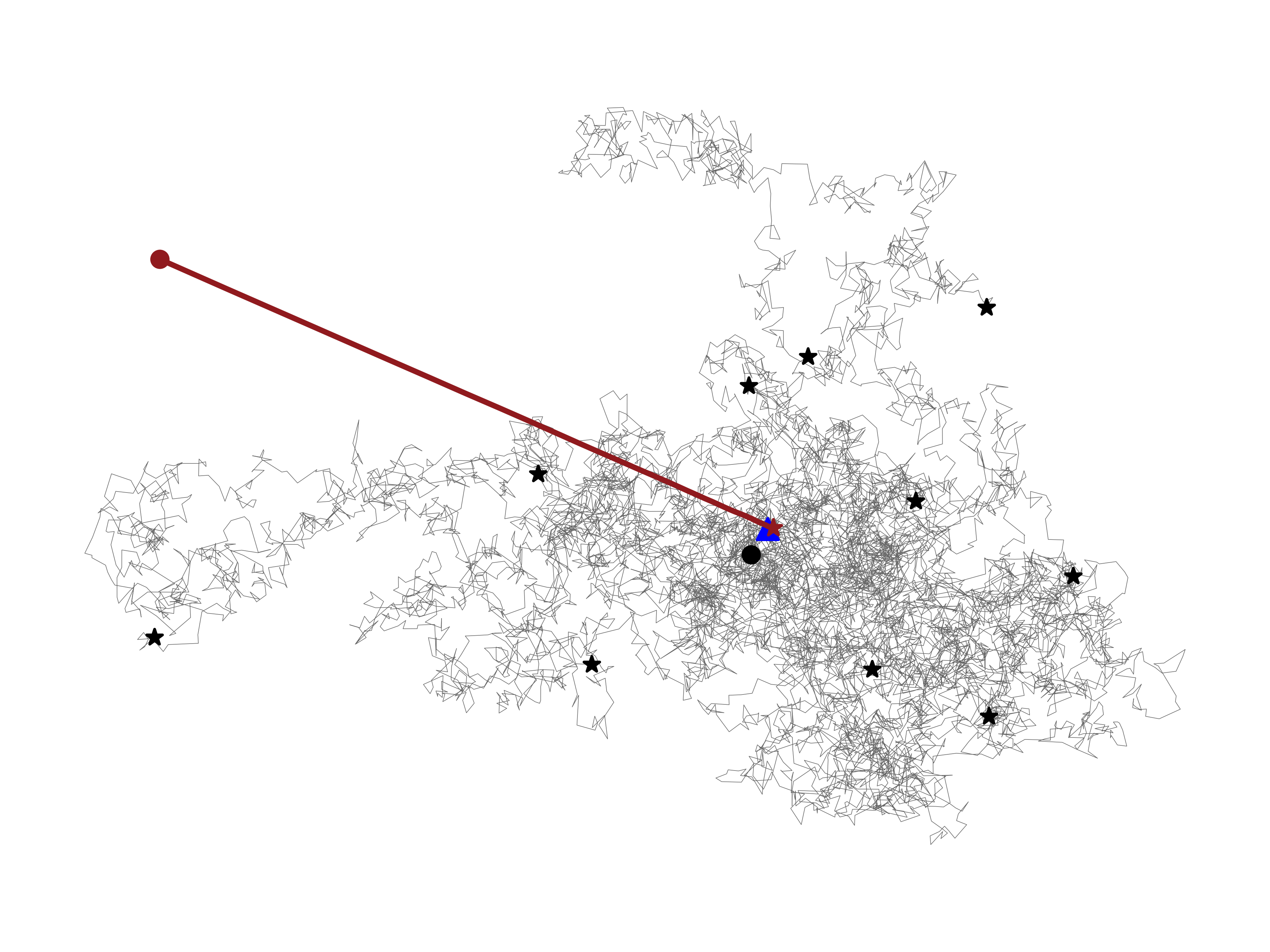
Figure 3: Black stars illustrate observations of sampled Brownian motions initiated at the black circle at the origin. Red circle illustrates initial diffusion mean estimate (chosen arbitrarily). The joint log-likelihood of diffusion bridges from the current diffusion mean estimate to each of the observations is computed and the diffusion mean estimate is updated by gradient ascent on it. The red line shows the path taken by the diffusion mean estimate. Red star illustrates final diffusion mean estimate, which coincides almost fully with the true diffusion mean, indicated by the blue triangle.

6 APPLICATIONS

Two distinct biological applications are presented to exemplify the utility of the proposed methodology. Whereas the previous section, for demonstration purposes, utilised a simplified diffusion process — a Brownian motion — for which transition densities and the score are analytically known, this section uses the actual process of interest; Kunita flows.

A neural network is trained using the score matching technique presented in Section 3.3 to serve as a function approximator of the unknown score. This score approximation is then used in the proposed stable importance sampler.

The structure of the neural network is illustrated in Figure 4, exemplified here for handling 100 2-dimensional landmarks for e.g. the butterflies. One additional input component is added for the time step.

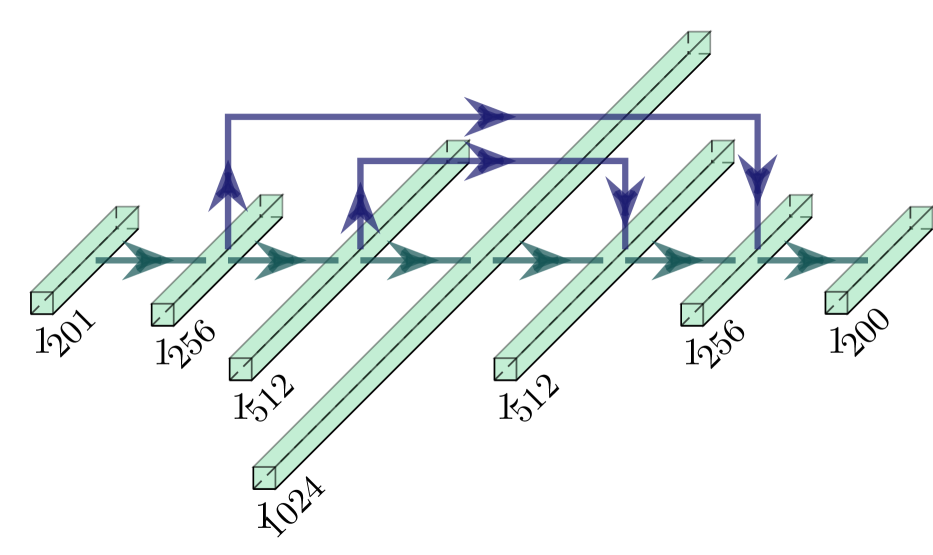
Figure 4: Structure of neural network used, shown here corresponding to 100-point two-dimensional landmark shape; the shape is flattened into a 200-dimensional vector and the time point is concatenated. The dark blue skip connections add the values element-wise to the later layers. These skip connections are found to help the model express the score fields properly.

To make a single network able to approximate scores for a range of variance parameters, the sinusoidal embedding of [17] is used for normalised log-variance parameters and included as a scale-shift operation on the down-sizing layers.

6.1 Relationships

The most likely variance parameter estimate for a diffusion bridge between two observations may informally be viewed as an indicator of similarity between the observations. Given e.g. archaeological observations, this similarity indication may provide pointers towards establishing relationships.

To demonstrate this, three observations of parietal bone outlines in canid skulls of known origin are considered; two from distinct specimens of Canis lupus (grey wolf) and one from a specimen of Vulpes vulpes (red fox). The outline of the parietal bone is chosen for its importance in skull structure and brain protection. Figure 5 illustrates two of these landmark configurations, along with learned diffusion bridges connecting them with different variance parameters for the assumed Kunita flow.

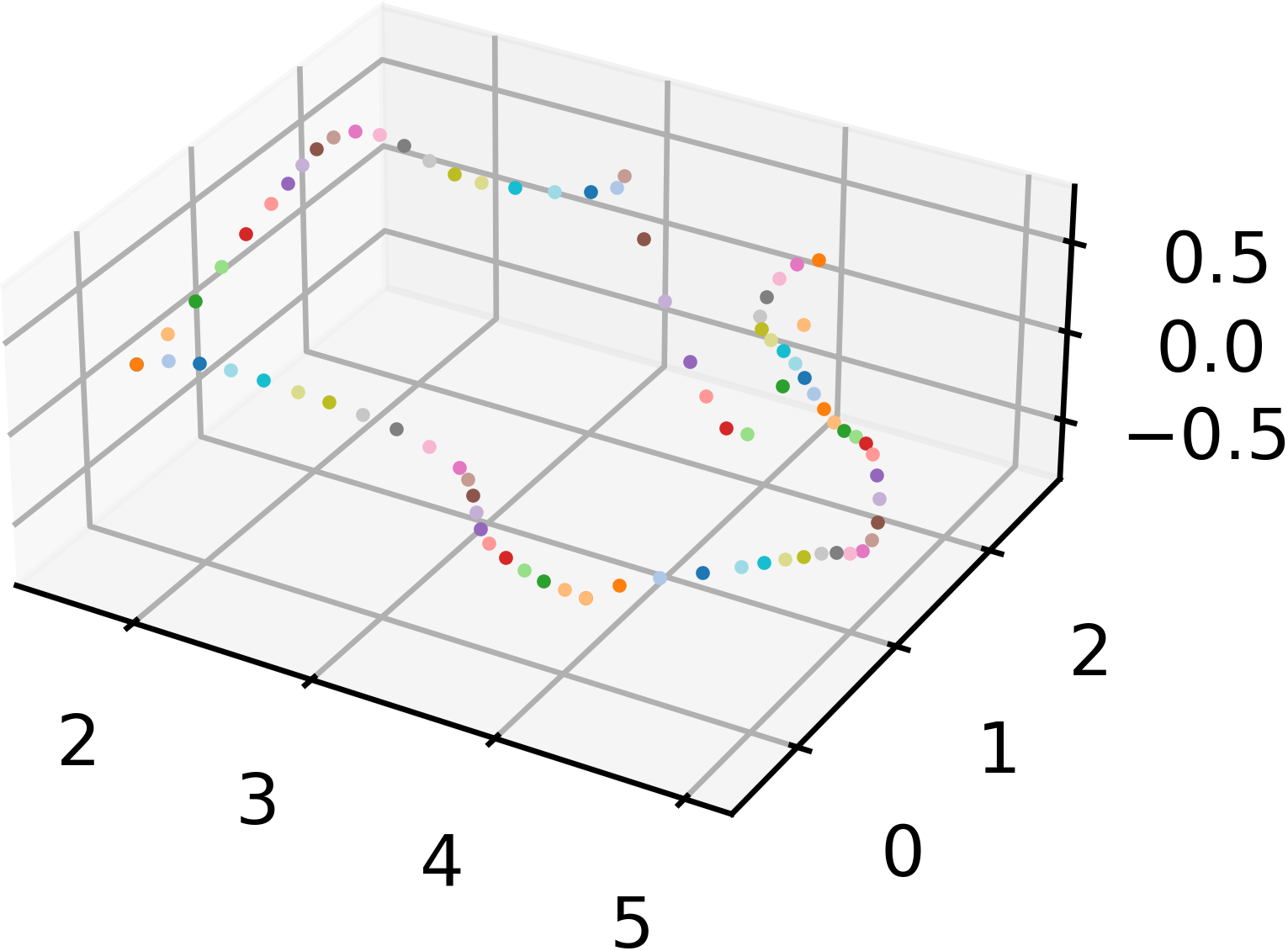
(a) Canis lupus

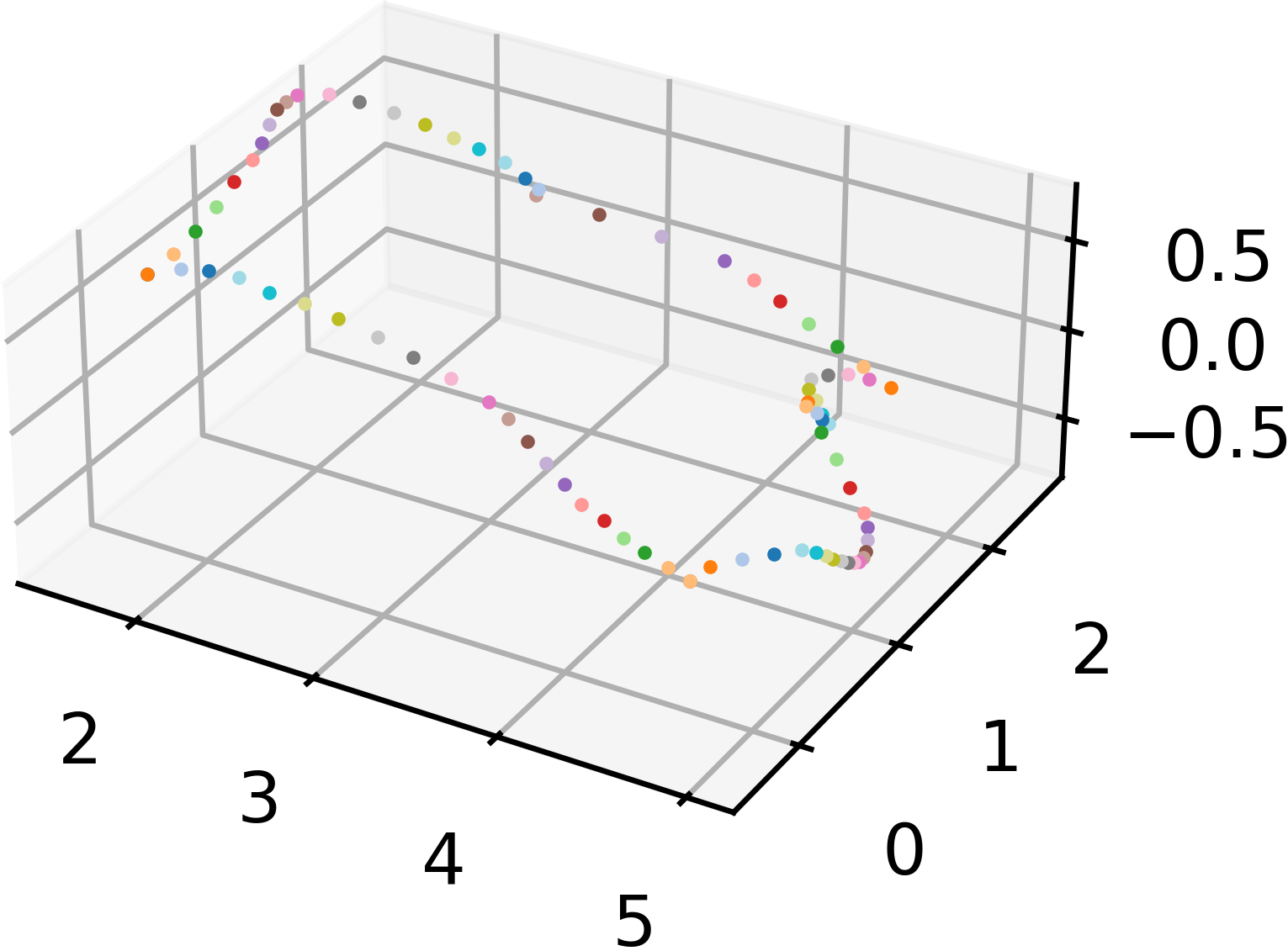
(b) Vulpes vulpes

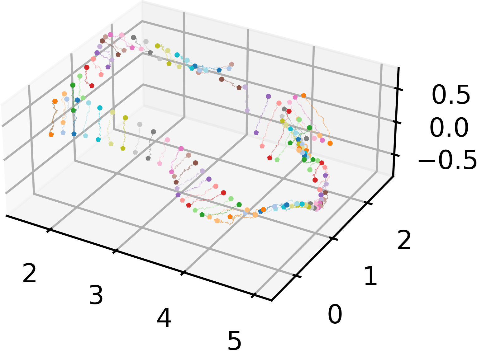
(c) bridge, $\sigma=0.0464$

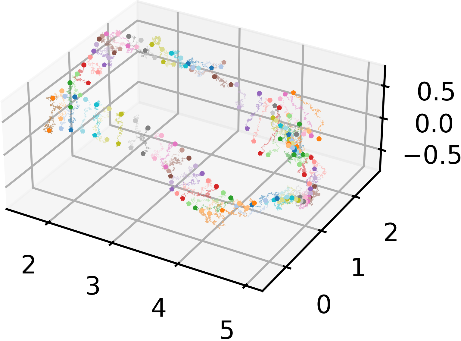
(d) bridge, $\sigma=0.129$

Figure 5: (a) and (b) illustrate landmark discretisations of the outline of the parietal bone of Canis lupus and Vulpes vulpes specimens, respectively. (c) and (d) show learned Kunita flow diffusion bridges between the landmark configurations of (a) and (b), using two different variance parameter values for the process. Data from [5].

Variance parameters are inferred for the diffusion bridges between the two wolves and between one wolf and the fox, respectively. Figure 6 illustrates the approximated (off-by-a-constant) log-likelihood curves, with most likely value indicated. Unsurprisingly, the inferred most likely variance parameter is larger for the inter-species bridges than for intra-species bridges — even after performing Procrustes alignment, eliminating size information.

Figure 6: Approximated (off-by-a-constant) log-likelihood curves for the bridges illustrated in Figure 5. Dashed vertical lines indicate most likely variance parameter value for each of the bridges, computed using learned score approximators in the proposed importance sampler.

Although expected, this result may serve as support for the proposed methodology, exactly because of how biologically obvious it is.

6.2 Ancestral State

Section 5.2 established estimation of diffusion means using the proposed methodology. For a collection of observations of extant species, their diffusion mean may serve as a most likely ancestral state candidate. Conditioning the neural network score approximator on initial state, and training on a distribution of initial states surrounding the collection of observations may allow such ancestral state reconstruction.

To illustrate this, six butterflies of the Papilio genus are chosen, with and without swallow tails. One of them is chosen arbitrarily as an initial diffusion mean estimate, and this estimate is then deformed by gradient ascent on the joint log-likelihood of the bridges from it to each observation. Figure 7 illustrates the progression of the mean estimate. Curiously, it moves towards the ancestral shape having swallow tails.

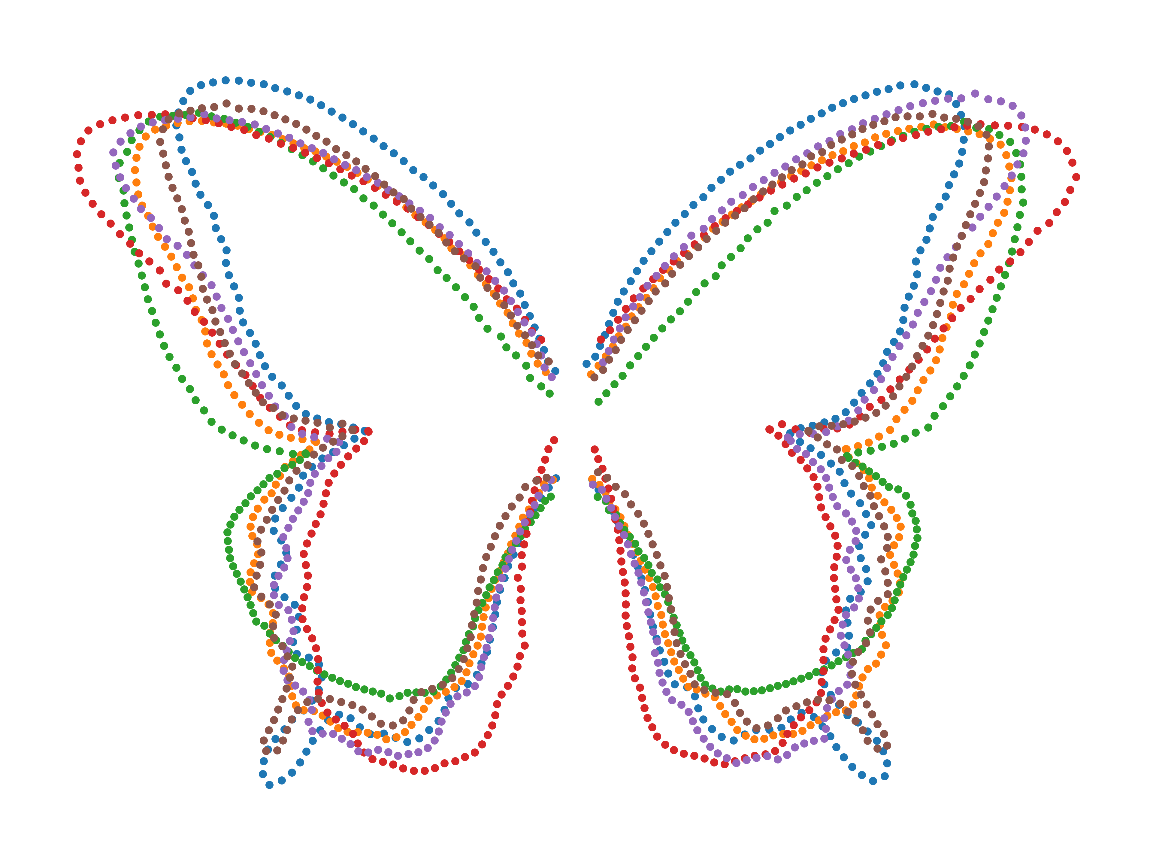
(a) observations

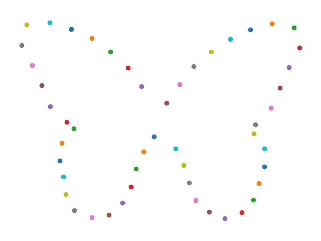
(b) initial estimate

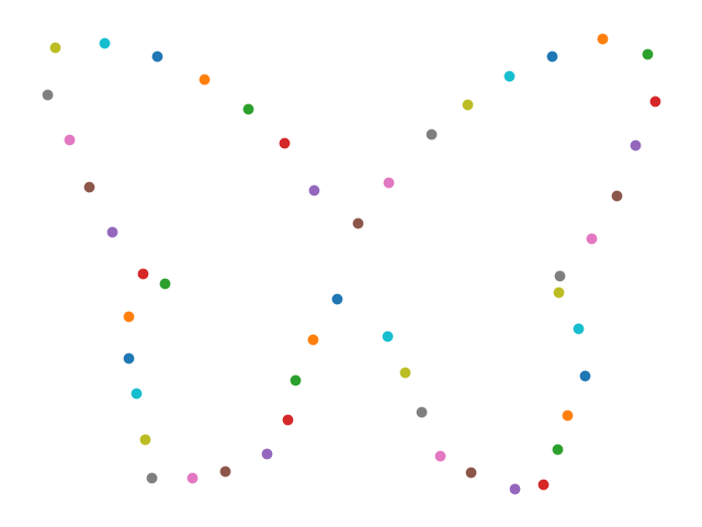
(c) after 150 steps

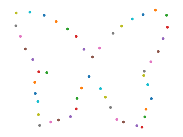
(d) after 300 steps

Figure 7: Ancestral shape reconstruction of six butterflies of the Papilio genus, shown in (a). One of them is chosen as an initial guess of their diffusion mean estimate, shown in (b). This estimate is updated via gradient ascent on the approximated log-likelihood of the diffusion bridges between the estimate and each of the observations. Plots (c) and (d) illustrate the progress of the diffusion mean estimate as an ancestral state reconstruction estimate. Notice how the ancestral state tends towards having swallow tails.

7 CONCLUSION

A differentiable likelihood estimation methodology capable of parameter inference and diffusion mean estimation in challenging, non-linear and high-dimensional diffusion processes has been presented. Powered by a symbiosis between modern deep learning — score matching via a novel numerically stable objective function — and theoretical statistics, it has been demonstrated how the proposed methodology is capable of delivering insights in the field of evolutionary biology.

We envision future work could investigate integrating this methodology on phylogenetic trees, as well as making neural networks conditioned on initial state more stable for better diffusion mean estimation.

Acknowledgements

The work presented in this article was done at the Center for Computational Evolutionary Morphometry and is partially supported by the Novo Nordisk Foundation grant NNF18OC0052000 as well as a research grant (VIL40582) from VILLUM FONDEN and UCPH Data+ Strategy 2023 funds for interdisciplinary research.

References

Data

Exact sources of the data used in this paper are presented in the table on the following page, which includes source of each species and where it was collected.

The canid skulls from Bergen were lent by Dr. Hanneke J.M. Meijer, Associate Professor & Curator of Osteology, University Museum of Bergen, Hanneke.Meijer@uib.no

type	Class	scientificName	locality	institutionCode	ID	Sex	Source
2d image	Insecta	Papilio ambrax Boisduval, 1832	13 km W of Kennedy	MCZ	89060	male	Gbif, [7]
2d image	Insecta	Papilio deiphobus Linnaeus, 1758	Seram [Ceram]	MCZ	211983	male	Gbif, [7]
2d image	Insecta	Papilio polyxenes asterius Stoll, 1782	Weston	MCZ	174079	male	Gbif, [7]
2d image	Insecta	Papilio protenor Cramer, 1775	-	MCZ	180722	male	Gbif, [7]
2d image	Insecta	Papilio polytes Linnaeus, 1758	Bacan Batjan, Batchian	MCZ	170907	male	Gbif, [7]
2d image	Insecta	Papilio slateri	North Borneo	MCZ	176631	male	Gbif, [7]
3d scan	Mammal	Canis lupus Linnaeus, 1758	Bergen	UIB	B2	-	EvoMorphoLab
3d scan	Mammal	Canis lupus Linnaeus, 1758	Bergen	UIB	2698	-	EvoMorphoLab
3d scan	Mammal	Vulpes vulpes Linnaeus, 1758	-	L-ahr	l-ahr:208049		Morphosource, [5]

Table 1: Source of each species. L-ahr: Laboratory of Adam Hartstone-Rose, MCZ: Havard Museum of Comparative Zoology, UIB: Bergen University Natural History Museum

References

- [1] Brian D.O. Anderson “Reverse-time diffusion equation models” In Stochastic Processes and their Applications 12.3, 1982, pp. 313–326 DOI: 10.1016/0304-4149(82)90051-5
- [2] Alexis Arnaudon, Darryl D. Holm, Akshay Sadananda Uppinakudru Pai and Stefan Horst Sommer “A stochastic large deformation model for computational anatomy” null ; Conference date: 25-06-2017 Through 30-06-2017 In Information Processing in Medical Imaging, Lecture notes in computer science Switzerland: Springer, 2017, pp. 571–582 DOI: 10.1007/978-3-319-59050-9˙45
- [3] Alexis Arnaudon, Darryl D. Holm and Stefan Sommer “A Geometric Framework for Stochastic Shape Analysis” In Foundations of Computational Mathematics 19.3 Springer ScienceBusiness Media LLC, 2018, pp. 653–701 DOI: 10.1007/s10208-018-9394-z
- [4] Alexis Arnaudon, Frank Meulen, Moritz Schauer and Stefan Sommer “Diffusion Bridges for Stochastic Hamiltonian Systems and Shape Evolutions” In SIAM Journal on Imaging Sciences 15.1 Society for Industrial & Applied Mathematics (SIAM), 2022, pp. 293–323 DOI: 10.1137/21m1406283
- [5] Doug M Boyer, Gregg F Gunnell, Seth Kaufman and Timothy M McGeary “Morphosource: archiving and sharing 3-D digital specimen data” In The Paleontological Society Papers 22 Cambridge University Press, 2016, pp. 157–181
- [6] Benjamin Eltzner, Pernille E.H. Hansen, Stephan F. Huckemann and Stefan Sommer “Diffusion means in geometric spaces” In Bernoulli 29.4 Bernoulli Society for Mathematical StatisticsProbability, 2023, pp. 3141–3170 DOI: 10.3150/22-BEJ1578
- [7] GBIF “Occurrence Download” The Global Biodiversity Information Facility, 2023 DOI: 10.15468/DL.PDHSZ3
- [8] Jeremy Heng, Valentin De Bortoli, Arnaud Doucet and James Thornton “Simulating Diffusion Bridges with Score Matching”, 2022 arXiv:2111.07243 [stat.CO]
- [9] Patrick Kidger “On Neural Differential Equations”, 2021
- [10] Hiroshi Kunita “Stochastic flows and stochastic differential equations ” In Stochastic flows and stochastic differential equations, Cambridge studies in advanced mathematics ; 24. Cambridge: Cambridge University Press, 1990
- [11] Ming Lin, Rong Chen and Per Mykland “On Generating Monte Carlo Samples of Continuous Diffusion Bridges” In Journal of the American Statistical Association 105.490 Taylor & Francis, 2010, pp. 820–838 DOI: 10.1198/jasa.2010.tm09057
- [12] Asger Roer Pedersen “Consistency and Asymptotic Normality of an Approximate Maximum Likelihood Estimator for Discretely Observed Diffusion Processes” In Bernoulli 1.3 International Statistical Institute (ISI)Bernoulli Society for Mathematical StatisticsProbability, 1995, pp. 257–279
- [13] Asger Roer Pedersen “A New Approach to Maximum Likelihood Estimation for Stochastic Differential Equations Based on Discrete Observations” In Scandinavian Journal of Statistics 22.1 [Board of the Foundation of the Scandinavian Journal of Statistics, Wiley], 1995, pp. 55–71
- [14] “Riemannian Geometric Statistics in Medical Image Analysis” United States: Academic Press, 2020 DOI: 10.1016/C2017-0-01561-6
- [15] Simo Särkkä and Arno Solin “Applied Stochastic Differential Equations”, Institute of Mathematical Statistics Textbooks Cambridge University Press, 2019
- [16] Stefan Sommer, Alexis Arnaudon, Line Kuhnel and Sarang Joshi “Bridge Simulation and Metric Estimation on Landmark Manifolds”, 2017 arXiv:1705.10943 [cs.CV]
- [17] Ashish Vaswani, Noam Shazeer, Niki Parmar, Jakob Uszkoreit, Llion Jones, Aidan N Gomez, Łukasz Kaiser and Illia Polosukhin “Attention is All you Need” In Advances in Neural Information Processing Systems 30 Curran Associates, Inc., 2017
Data