A Priori Error Bounds and Parameter Scalings for
the
Time Relaxation Reduced Order Model
Abstract
The a priori error analysis of reduced order models (ROMs) for fluids is relatively scarce. In this paper, we take a step in this direction and conduct numerical analysis of the recently introduced time relaxation ROM (TR-ROM), which uses spatial filtering to stabilize ROMs for convection-dominated flows. Specifically, we prove stability, an a priori error bound, and parameter scalings for the TR-ROM. Our numerical investigation shows that the theoretical convergence rate and the parameter scalings with respect to ROM dimension and filter radius are recovered numerically. In addition, the parameter scaling can be used to extrapolate the time relaxation parameter to other ROM dimensions and filter radii. Moreover, the parameter scaling with respect to filter radius is also observed in the predictive regime.
keywords:
Reduced order model, Stabilization, Spatial filter, Time relaxationMSC:
[2020] 65M12 , 65M15 , 65M60 , 65M70 , 76D05 , 76F99[VT]organization=Department of Mathematics,addressline = Virginia Tech, city= Blacksburg, postcode=24060, state=VA, country=USA
[UAM]organization=Department of Mathematics,addressline =Universidad Autonoma de Madrid, city= Madrid, postcode=24060, state=VA, country=Spain
1 Introduction
The incompressible Navier-Stokes equations (NSE) are
| (1) | ||||
| (2) |
where and are the velocity and pressure fields, respectively, defined on the spatial domain, , and the time interval, . is an external force, and is the inverse of the Reynolds number. Appropriate boundary and initial conditions are needed to close the system.
Fluid flows at high Reynolds numbers exhibit a wide range of spatial and temporal scales that make their direct numerical simulation (DNS) often impractical [1, 2]. This leads to the need of alternative computational approaches, such as large eddy simulations (LES), Reynolds-averaged Navier–Stokes equations (RANS), and numerical regularizations. One type of regularization is the time relaxation model (TRM) [3, 4], which leverages spatial filtering to increase the numerical stability. The TRM for a domain , , and for is given as
| (3) | ||||
| (4) |
where the dimensionless parameter is called the time relaxation parameter, which is often manually tuned to adjust the numerical stabilization, and is a regularization term defined in Section 2. The goal of is to drive the unresolved fluctuations of down to . TRM has been investigated in [5, 6, 7, 8, 9, 10, 11] and has been used in various applications [12, 13]. A TRM review can be found in [14].
Although the DNS computational cost is significantly reduced by LES, RANS, and numerical stabilization, these approaches remain computationally prohibitive in decision-making applications where multiple forward simulations are needed. In those cases, reduced order models (ROMs) represent efficient alternatives. ROMs are computational models whose dimension is orders of magnitude lower than the dimension of full order models (FOMs), i.e., models obtained from classical numerical discretizations. In the numerical simulation of fluid flows, Galerkin ROMs (G-ROMs), which use data-driven basis functions in a Galerkin framework, have provided efficient and accurate approximations of laminar flows, such as the two-dimensional flow past a circular cylinder at low Reynolds numbers [15, 16]. However, turbulent flows are notoriously hard for the standard G-ROM. Indeed, to capture the complex dynamics, a large number [17] of ROM basis functions is required, which yields high-dimensional ROMs that cannot be used in realistic applications. Thus, computationally efficient, low-dimensional ROMs are used instead. Unfortunately, these ROMs are inaccurate since the ROM basis functions that were not used to build the G-ROM have an important role in dissipating the energy from the system [18]. Indeed, without enough dissipation, the low-dimensional G-ROM generally yields spurious numerical oscillations. Thus, closures and stabilization strategies are required for the low-dimensional G-ROMs to be stable and accurate [18, 19, 20, 21, 22, 23].
FOM stabilizations and closures are supported by thorough numerical analysis, particularly when applied alongside traditional methods like the finite element method (FEM) or SEM [1, 24, 25, 26]. These references address both fundamental numerical analysis issues, such as stability and convergence, and practical challenges, like determining appropriate parameter scalings for stabilization coefficients. These two aspects are closely linked, as insights from numerical analysis guide the selection of parameter scalings, which inform practical decisions. We emphasize, however, that despite growing interest in ROM closures and stabilizations, their comprehensive mathematical and numerical analysis remains an open challenge. Indeed, while some strides have been made in analyzing ROM closures and stabilizations [27, 28, 29, 30, 31, 32, 33], much work is needed to reach the rigor of FOM analysis.
In this paper, we take a step in this direction by establishing the first rigorous numerical analysis results, including stability and a priori bounds, for the time relaxation reduced order model (TR-ROM), which was successfully used in [34] in numerical simulations of turbulent channel flow. Crucially, we also derive parameter scalings that ensure ROM parameters automatically adjust with changes in the corresponding FOM and ROM parameters, eliminating the need for manual tuning often required in existing data-driven ROMs.
This article is organized as follows: In Section 2, we give preliminaries about the SEM, G-ROM, and ROM filtering. In Section 3, we present the TR-ROM, prove its unconditional stability and an a priori error bound, and derive novel scalings for the time relaxation parameter. In Section 4, we show that the theoretical convergence rates and parameter scalings with respect to ROM dimension and filter radius are numerically recovered for the 2D flow past a cylinder and 2D lid-driven cavity. In Section 5, we present the conclusions of our theoretical and numerical investigations.
2 Notations and Preliminaries
2.1 Spectral Element Method
This paper will use the following spaces: , , and , where for domain . The norm is denoted as , with the corresponding inner product . Vector-valued functions are indicated in boldface having components ( or ). The norm will be denoted by , with all other norms clearly denoted. For the continuous vector function defined on the entire time interval , we have
The solutions are sought in the following functional spaces:
Boldface indicates that the space is spanned by vector-valued functions. The dual space of is denoted as , and the norm of the space is . Moreover, we define to be the weakly divergence-free subspace of .
The FOM is based on the SEM in the open-source code Nek5000 [35], and uses the – velocity-pressure coupling [36]. To this end, let be a polygonal domain and be a conforming partition of into rectangles or rectangular parallelepipeds. If is a function defined in , the restriction of to will be denoted by . We set
where denotes the space of polynomials of degree less or equal to with respect to each variable. The discrete space of pressures is defined as
The discrete velocity belongs to the space
With the above choice for the space of pressures, the following - condition is satisfied [37, 38],
| (5) |
where is a constant that does not depend on .
Let denote the time step, and , , the time instances. We also use the notation and the following discrete norms:
For , we define the trilinear forms as follows:
| (6) | |||||
| (7) |
The following approximation properties hold [37, 38]:
| (8) | ||||
| (9) | ||||
| (10) |
We also use the following lemmas:
Lemma 2.2 (Discrete Gronwall Lemma [41]).
Let , H, and (for integers ) be finite nonnegative numbers such that
Suppose that . Then,
Let be the velocity of the Navier-Stokes equations for a given initial condition, and let be its continuous in time spectral element approximation. Then, the following bound for the error is proved in [42] (see Remarks 4.2 and 4.3):
assuming ().
Using standard techniques, one can also prove error bounds for the fully discrete method. In particular, we will make the following assumption:
Assumption 2.1 (Spectral Element Error).
Remark 2.1.
As discussed in [43], is used to ensure that the imaginary eigenvalues associated with skew-symmetric advection operator are within the stability region of the BDF/EXT time-stepper.
2.2 Galerkin Reduced Order Model (G-ROM)
In this section, we introduce the G-ROM. We follow the standard proper orthogonal decomposition (POD) procedure [44, 45] to construct the reduced basis function. To this end, we collect a set of spectral element (FOM) solutions lifted by the zeroth mode . The POD method seeks a low-dimensional basis in that optimally approximates the snapshots, that is, solves the minimization problem:
subject to the conditions , for , where is the Kronecker delta. The minimization problem can be solved by considering the eigenvalue problem , for , where is the snapshot Gramian matrix using the inner product (see, e.g., [21, 46] for alternative strategies).
The first POD basis functions are constructed from the first eigenmodes of the Gramian matrix. The G-ROM is then constructed by inserting the POD approximated solution into the weak form of the NSE: Find such that, for all ,
| (14) |
where is the ROM space.
It can also be shown that the following error formula holds for the -POD basis functions [47]:
| (15) |
where is the rank of the Gramian matrix, .
Remark 2.2.
Because the POD basis functions are a linear combination of the snapshots generated from the FOM, the POD basis functions satisfy the boundary conditions of the original PDE and inherit the FOM’s divergence-free properties. In this paper, the FOM is based on a SEM discretization, which yields only a weakly divergence-free velocity. More precisely, the POD basis functions belong to , giving . Thus, to ensure the ROM stability in Lemma 3.1, we equip the ROM with the skew-symmetric trilinear form in (7).
Additionally, we make use of the following definitions and lemmas:
Definition 2.1 (ROM Projection).
Let such that, is the unique element of satisfying
| (16) |
Lemma 2.3 ( POD Projection error).
The POD projection error in the norm satisfies
| (17) |
Proof.
These sharper bounds can be obtained by using the inner product and norm instead of the inner product and norm in [31, Lemma 3.2]. ∎
We list a POD inverse estimate, which will be used in what follows. Let with be the POD stiffness matrix. Let denote the matrix 2-norm. Since this is traditional notation, in what follows we will use the notation both for the norm and for the matrix 2-norm. It will be clear from the context which norm is used.
Lemma 2.4 (POD Inverse Estimates [33]).
For all , the following POD inverse estimate holds:
| (18) |
The inverse estimate (18) was proved in Lemma 2 and Remark 2 in [48]. The scaling of with respect to was numerically investigated in Remark 3.3 in [49] and in Remark 3.2 in [27].
Lemma 2.5 ( Stability of of ROM Projection [33]).
For all , the ROM projection satisfies
| (19) |
The following error bound is a slightly modified variation of [31, Lemma 3.3]. This is due to our different spectral element error Assumption 2.1 and different Lemma 2.3. Furthermore, we assume a third-order in time discretization (i.e., BDF3/EXT3) as opposed to the first-order backward Euler method.
Lemma 2.6 (Modified Lemma 3.3 in [31]).
For any , its projection, , satisfies the following error bounds:
| (20) | |||
| (21) |
Proof.
A generalization of Lemma 2.6 is given by Corollary 2.0.1. This allows a modularity of the projection error to accommodate different discretizations of the FOM.
Corollary 2.0.1.
For any , its projection, , satisfies the following error bounds:
| (22) | ||||
| (23) |
where is the solution given by the full order model (e.g. FEM, SEM, etc).
We also assume the following bounds, analogous to those in [49]:
Assumption 2.2.
For any , where , its projection, , satisfies the following error estimates:
| (24) | ||||
| (25) |
Remark 2.3 (See also Remark 3.1 in [50].).
The pointwise in time error bounds in Assumption 2.2 are needed in the proof of Theorem 3.1. Specifically, we use those bounds to prove inequalities (49) and (51). We emphasize that using instead the average error bounds in Lemma 2.6 in the proof of Theorem 3.1 would yield suboptimal error bounds (see also [50, Remark 3.1 and Lemma 4.2]).
Assumption 2.2 and its important effect on the optimality of a priori error bounds was carefully discussed in [51] (see also [31, Remark 3.2]). In particular, it was shown in [51] that using both the snapshots and the snapshot difference quotients to construct the ROM basis yields optimal error bounds without making Assumption 2.2. This result was further improved in [52, 53], where optimal error bounds were proven using only the snapshot difference quotients and the snapshot at the initial time or the mean value of the snapshots. Further improvements were recently presented in [54].
For simplicity, in this paper we do not include the snapshot difference quotients, and instead assume the pointwise in time error bounds in Assumption 2.2.
2.3 ROM filtering
We formally introduce the time relaxation term , where denotes the spatially averaged representation of . Analogous to what was done for the continuous differential filter [55, 56] and discrete differential filter [57], we define the ROM differential filter as follows: For and a given filter width , we let be defined by , where is the unique solution of the following variational problem:
| (26) |
We note that, when the ROM basis is generated by using the POD strategy, the ROM basis functions (and, thus, the ROM solution) inherit the weakly divergence-free property from the FOM. Leveraging this fact, we do not need to use a Stokes filter, which has been used for weekly preservation of incompressibility [58, 59], and utilize instead as defined in equation (26).
Lemma 2.7.
(ROM Filtering Error Estimate [33]) For , the ROM filter satisfies
| (27) |
Remark 2.4.
The proof of Lemma 2.7 follows along the same lines as the proof of Lemma 4.3 in [33]. The main difference is that one needs to use SEM estimates (Assumption 2.1) instead of FEM estimates. Furthermore, as pointed out in [33, Remark 4.1], since the stability of the projection is not available in a ROM setting, the better scalings of the seminorm of the filtering error in [60] cannot be extended to the ROM setting in a straightforward manner.
It is easy to check that is symmetric and semi-positive definite. The operator is also compact and . Its associated eigenvalues satisfy It is also easy to check that is symmetric, semi-positive definite, and compact. Moreover, its eigenvalues are so that . Finally, it is easy to check that implies , so that is not an eigenvalue of , and then is strictly positive definite. This allows us to define the norm:
| (28) |
More details on this can be found in [8, Lemma 2.1].
3 Stability and Error Bounds
In this section, we formally introduce our fully discrete TR-ROM. First, in Lemma 3.1, we prove unconditional stability of the new TR-TOM. Then, in Theorem 3.1, we prove an a priori error bound for the TR-ROM. Finally, in Section 3.1, we leverage the error bound in Theorem 3.1 to prove parameter scalings for the TR-ROM relaxation parameter, .
The fully discrete formulation of the TR-ROM is as follows: For , find satisfying
| (29) |
We assume that is the projection of into i.e., .
To prove the TR-ROM’s unconditional stability in Lemma 3.1, we adapt the approach in [5, 61, 62, 10] to the ROM setting.
Lemma 3.1.
The solution to the TR-ROM given by (29) is unconditionally stable: For any , the solution satisfies:
| (30) |
Proof.
Choosing in (29) yields
since the skew-symmetric nonlinear term vanishes. After using Cauchy-Schwarz and Young’s inequalities, the dual norm of , and (28), we have
Rearranging some terms and multiplying by , we obtain
Because is the projection of onto , summing over time steps yields the following stability bound:
| (31) |
∎
To prove the a priori error bound in Theorem 3.1, we extend the strategy in [5, 10, 62] to the ROM setting.
Theorem 3.1.
Let be the solution of the TR-ROM (29), with being the true solution of NSE (1)-(2), and let . Under the SE Assumption 2.1, ROM projection Assumption 2.2, and for sufficiently small , we have:
| (32) |
where depends exponentially on , depends on , , , , , , , but not on , , , , or , and is defined in (50).
Proof.
First, in (3) we introduce a weak formulation of the NSE: Find satisfying for all
| (33) |
We split the error in the usual way as , where and , with being the projection of in . Subtract equation (29) from the weak form of the NSE (3) evaluated at to obtain
Note that the nonlinear terms can be rewritten as
Using the above equality, splitting the error, letting , and noting that
, we obtain
| (34) | |||
We now bound the above terms. By Definition 2.1, , which yields
| (35) |
The next five terms are all bounded using standard methods.
| (36) | |||||
| (37) | |||||
| (38) | |||||
| (39) | |||||
| (40) | |||||
For the pressure term, since , can be subtracted and then bounded in the standard way:
| (41) |
For , we use the fact that , and Cauchy-Schwarz, Poincare-Friedrichs, and Young’s inequalities:
| (42) |
For , we use again Cauchy-Schwarz, Young’s, and Poincare-Friedrichs inequalities:
| (43) |
Substituting the bounds (35)-(43) into (34), multiplying by , summing up from to , and recalling that since , yields:
| (44) | |||||
Next, we continue to bound the error terms on the right-hand side of (44). Using the approximation properties (10), (20), and (21), we obtain:
| (45) | |||
| (46) |
| (47) | ||||
| (48) |
For the next bound, we use (21) and Assumption 2.2, resulting in:
| (49) |
For notational convenience, we denote all but the last term in (49) as
| (50) |
The following term utilizes the stability result from Lemma 3.1 together with the Cauchy-Schwarz inequality and Assumption 2.2
| (51) |
Using Lemma 2.7, we have the following bound:
| (52) |
Thus, using the above bounds, (44) becomes
| (53) |
Hence, by the Gronwall inequality from Lemma 2.2 with sufficiently small, i.e., , we obtain the following result:
| (54) |
The triangle inequality finishes the proof. ∎
3.1 Parameter Scalings
In this subsection, we build upon the error bound proved in Theorem 3.1 to derive parameter scalings for the time relaxation constant, . To discover the optimal choice of parameter , we extend the strategy used in [27] to the ROM setting. To this end, we consider the error bound given by the result of Theorem 3.1:
| (55) |
First, we note that following the classical approach (see, e.g., [27]) and attempting to minimize the whole left hand side of (55) would result in only the trivial solution . Choosing , however, would result in removing the time-relaxation term, which would yield the standard G-ROM. This would clearly be an impractical choice since G-ROM is notoriously inaccurate in the under-resolved regime. Thus, we propose a different strategy and minimize only the time-relaxation term (i.e., the third term) on the LHS of (55). Our choice is further motivated by [63], where it is stated that measures the high frequency components of , which is where spurious oscillations concentrate in the under-resolved regime. To minimize the time-relaxation term, we drop the other two terms on the LHS of (55), and divide by . To simplify the notation of the RHS of (55), we define a function as follows:
| (56) |
where
Taking the derivative of with respect to in (56) yields
| (57) |
Since , setting in (57) results in
| (58) |
Solving for in (58) gives the optimal parameter scaling for :
| (59) |
4 Numerical Results
In this section, we perform a numerical investigation of the theoretical results obtained in Section 3. To this end, we investigate whether the TR-ROM a priori error bound in Theorem 3.1 is recovered numerically. In addition, for the theoretical parameter scaling of the time-relaxation constant (59) derived in Section 3.1, we investigate if the time-relaxation parameter scalings with respect to the filter radius, , and ROM dimension, , are recovered numerically. The numerical investigation is performed for two test problems: the 2D flow past a circular cylinder at Reynolds number (Section 4.2), and the 2D lid-driven cavity at Reynolds number (Section 4.3).
The numerical investigation in this section focuses on the TR-ROM a priori error bound (32) in Theorem 3.1, which depends on the parameters , , , and , as well as the ROM truncation errors and defined in (15) and (17). In our numerical investigation, to measure the TR-ROM accuracy, we use the mean squared errors defined below:
| (60) |
where is the TR-ROM approximation, and is the ROM projection (Definition 2.1) onto the -dimensional reduced space. Specifically, we numerically investigate the rates of the convergence of and with respect to the ROM truncation errors and , respectively.
Remark 4.1.
The TR-ROM errors in (60) are computed with respect to the projected FOM solution because (i) the considered model problems do not have exact solutions, and (ii) the cost for computing the errors with respect to the projected FOM solution is independent of the number of FOM degrees of freedom, . Measuring the error with respect to the FOM solution would require a post-processing step. The value is selected so that the error between and is small.
4.1 TR-ROM Computational Implementation
The fully discrete formulation TR-ROM (29) is equivalent to the following system:
| (61) | ||||
| (62) |
Equations (61)–(62) are equivalent to the following algebraic system:
| (63) | ||||
| (64) |
where , , and are the reduced mass, stiffness, and advection operators. is the forcing vector projected onto the reduced space, and is the filter radius. The algebraic system (63)–(64) can be further expressed in a matrix-vector form:
| (65) |
where is a linear operator defined as The nonlinear system (65) is of size . However, using the relation, the nonlinear system (65) can be simplified to the following nonlinear system:
| (66) |
where the low-dimensional () matrix can be precomputed. We note that here we assumed that the zeroth mode, , is a zero velocity field, but the conclusion of simplifying the nonlinear system to size of still holds if one has a nontrivial zeroth mode.
We use the open-source code NekROM [64] to construct and solve the TR-ROM defined in (66) for the two test problems described below. We mention that, in the current TR-ROM implementation, the convection term is not in the skew-symmetric form . We note, however, that using the standard trilinear form does not have a significant impact on the code’s numerical stability.
4.2 2D Flow Past a Cylinder
Our first test problem is the 2D flow past a cylinder at Reynolds number , which is a canonical test case for ROMs. The computational domain is , where is the cylinder diameter, and the cylinder is centered at .
The reduced basis functions are constructed by applying the POD procedure to snapshots . The snapshots are collected in the time interval (measured in convective time units, , where is the free-stream velocity), after the von Karman vortex street is developed, with sampling time . The zeroth mode, , is set to be the FOM velocity field at . TR-ROM is simulated on the same time interval where the snapshots are collected. Thus, we are in the reproduction regime. As the initial condition for the TR-ROM, we choose the zero vector.
4.2.1 Rates of Convergence
We first investigate the rates of convergence of and with respect to and in the reproduction regime. To this end, we fix , and vary . Table 1 shows the magnitude of each term on the right-hand side of the theoretical error estimate (32) with these parameter values. Thus, the theoretical error estimate (32) yields the following rates of convergence:
| (67) |
| 2 | 6.94e-03 | 4.00e-06 | 1.02e-07 | 1.93e-06 | 2.47e+01 | 6.04e+03 | 6.94e-03 | 1.47e-04 | 5.91e+04 |
|---|---|---|---|---|---|---|---|---|---|
| 5 | 6.94e-03 | 4.00e-06 | 1.02e-07 | 1.93e-06 | 4.81e+00 | 2.63e+03 | 6.94e-03 | 8.47e-04 | 5.73e+04 |
| 10 | 6.94e-03 | 4.00e-06 | 1.02e-07 | 1.93e-06 | 3.05e-02 | 1.43e+01 | 6.94e-03 | 2.30e-03 | 2.69e+02 |
| 20 | 6.94e-03 | 4.00e-06 | 1.02e-07 | 1.93e-06 | 4.19e-05 | 1.35e-02 | 6.94e-03 | 9.34e-03 | 1.73e-01 |
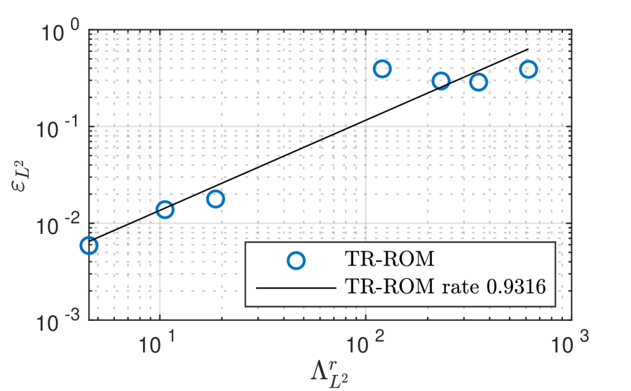
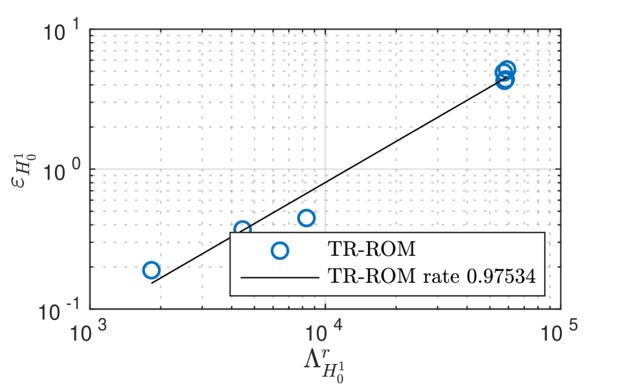
The behavior of the TR-ROM approximation errors and with respect to and , respectively, is shown in Figs. 1(a)–1(b). In these plots, the ranges of values for and correspond to the chosen range of values for , i.e., from to . The linear regression in the figures yields the following TR-ROM approximation error rates of convergence with respect to and :
| (68) |
Thus, the theoretical rates of convergence (67) are numerically recovered.
4.2.2 Scaling of with respect to
In Section 3.1, a theoretical formulation for the time-relaxation constant (59) is derived. With , and , the terms are relatively small. Hence, (59) can be further simplified as follows:
| (69) |
Given an value, , , , and are fixed. Hence, (69) indicates that the theoretical , , scales like either or , depending on the value. That is, there exist two values, and , such that
| (70) | ||||
| (71) | ||||
| (72) |
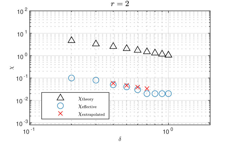
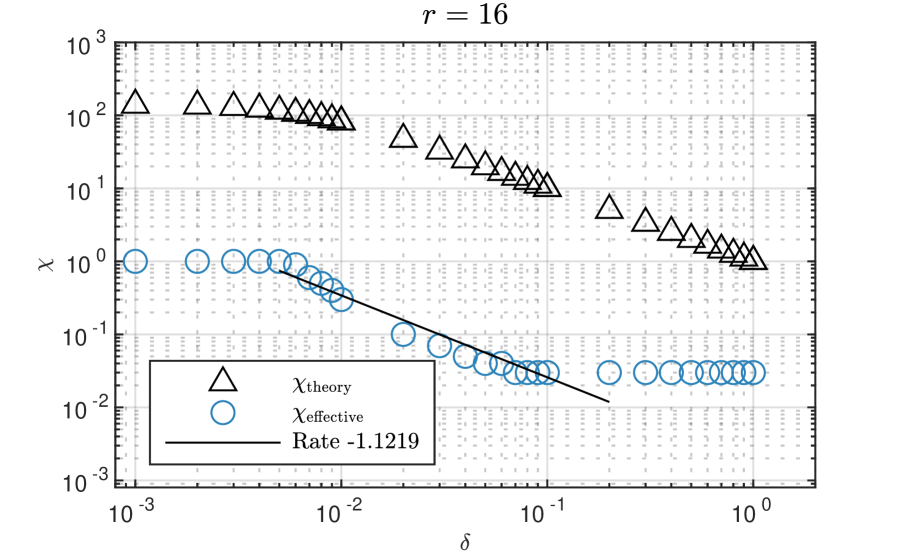
We investigate whether the scaling of the effective , , with respect to the filter radius, , follows the scaling indicated by (69).
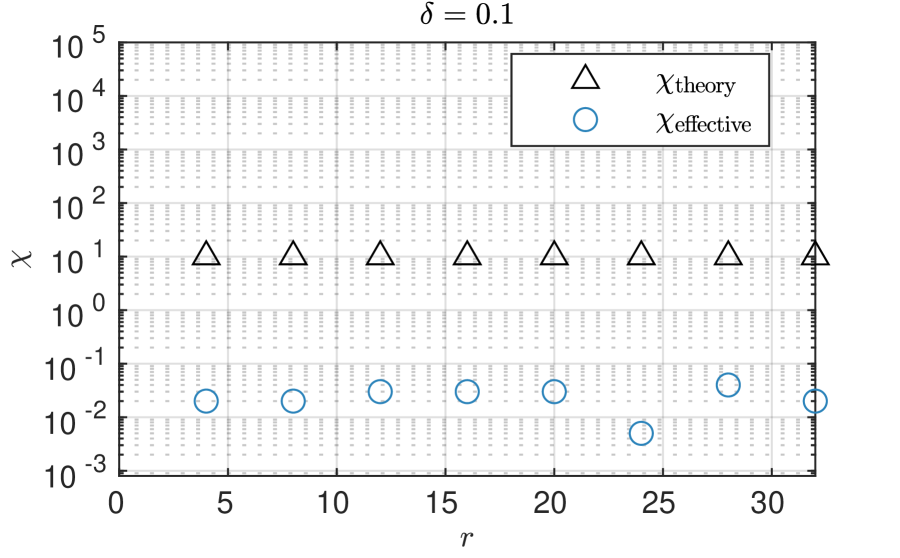
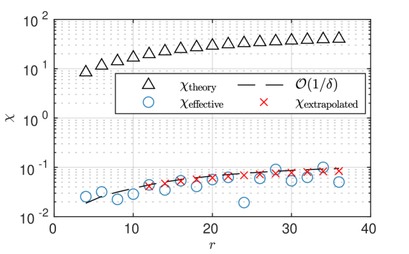
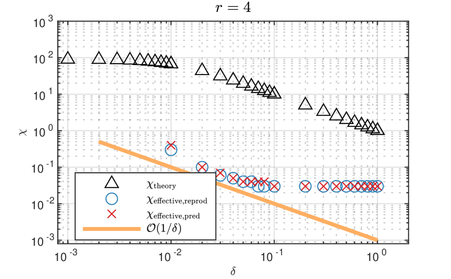
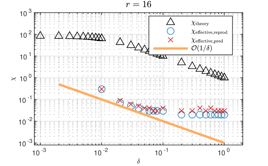
In Fig. 2, the behavior of in (69) and with respect to the filter radius, , is shown for . is found by solving the TR-ROM and is defined to be the largest value that yields an accuracy that is similar to (i.e., within of) the accuracy for the optimal , which is defined to be the value that yields the smallest . Specifically, for each value, we consider values from . For each value, values from are considered, and is selected from the values.
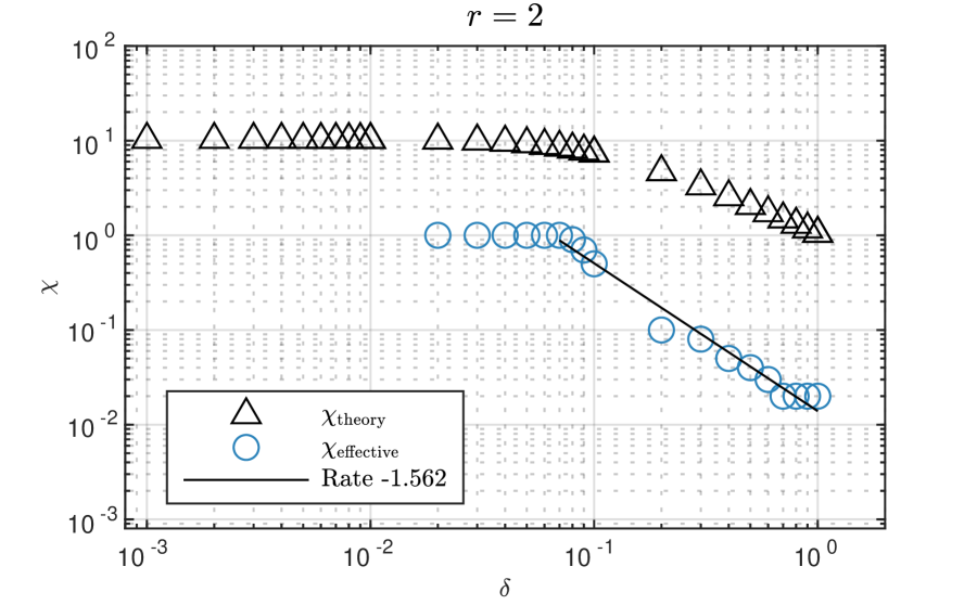
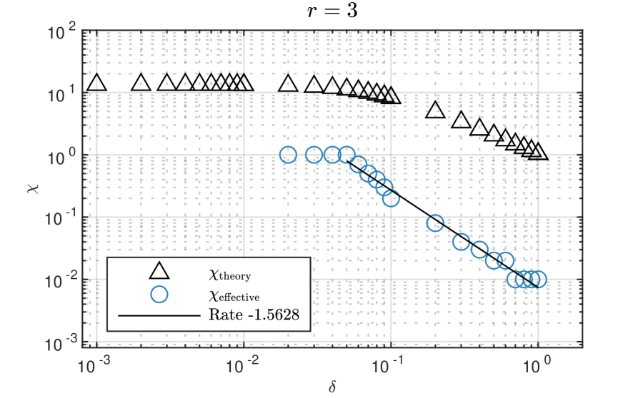
The results show that, for both values, scales like a constant for , where varies with the value. The linear regression in the figure indicates that scale like for .
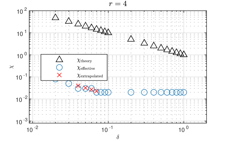
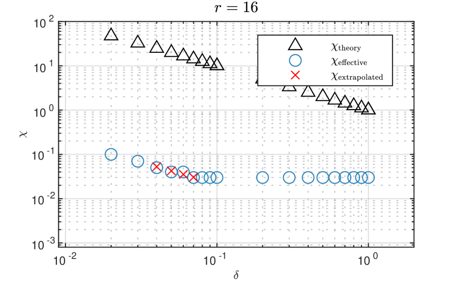
Next, we use two values to estimate the ratio between the effective and the theoretical (69), and demonstrate that this ratio can be used with to predict at other values. To this end, we compute the ratio between and at and , and take the average of the two ratios. The extrapolated values at are then computed using and the average of the two ratios calculated above. From the results shown in Fig. 3, the extrapolated is close to the effective , which illustrates the predictive capabilities of the theoretical parameter scaling for in (69).
4.3 2D Lid-Driven Cavity
Our next example is the 2D lid-driven cavity (LDC) problem at , which is a more challenging model problem compared to the 2D flow past a cylinder. As demonstrated in [19], the problem requires more than POD modes for G-ROM to accurately reconstruct the solutions and QOIs. A detailed description of the FOM setup for this problem can be found in [21].
The reduced basis functions are constructed by applying POD to statistically steady state snapshots . The snapshots are collected in the time interval with sampling time . The zeroth mode, , is set to the FOM velocity field at .
4.3.1 Rates of Convergence
We first investigate the rates of convergence of and with respect to and , respectively. To this end, we fix , and vary . Table 2 shows the magnitude of each term on the right-hand side of the theoretical error estimate (32) with these choices of parameters.
| 2 | 1.56e-02 | 1.00e-06 | 3.24e-08 | 6.10e-07 | 4.30e-03 | 2.59e+02 | 1.56e-02 | 2.86e-01 | 3.92e+04 |
|---|---|---|---|---|---|---|---|---|---|
| 4 | 1.56e-02 | 1.00e-06 | 3.24e-08 | 6.10e-07 | 2.26e-03 | 1.35e+02 | 1.56e-02 | 3.39e-01 | 2.01e+04 |
| 8 | 1.56e-02 | 1.00e-06 | 3.24e-08 | 6.10e-07 | 1.30e-03 | 7.72e+01 | 1.56e-02 | 3.77e-01 | 1.14e+04 |
| 16 | 1.56e-02 | 1.00e-06 | 3.24e-08 | 6.10e-07 | 5.63e-04 | 3.14e+01 | 1.56e-02 | 4.42e-01 | 4.38e+03 |

The behavior of the TR-ROM approximation errors with respect to and with respect to , respectively, are shown in Figs. 4(a)–4(b). The ranges of and correspond to to . The linear regression in the figures indicates the following TR-ROM approximation error rates of convergence with respect to and :
| (73) |
Thus, the theoretical rates of convergence (67) are numerically recovered.
4.3.2 Scaling of with respect to
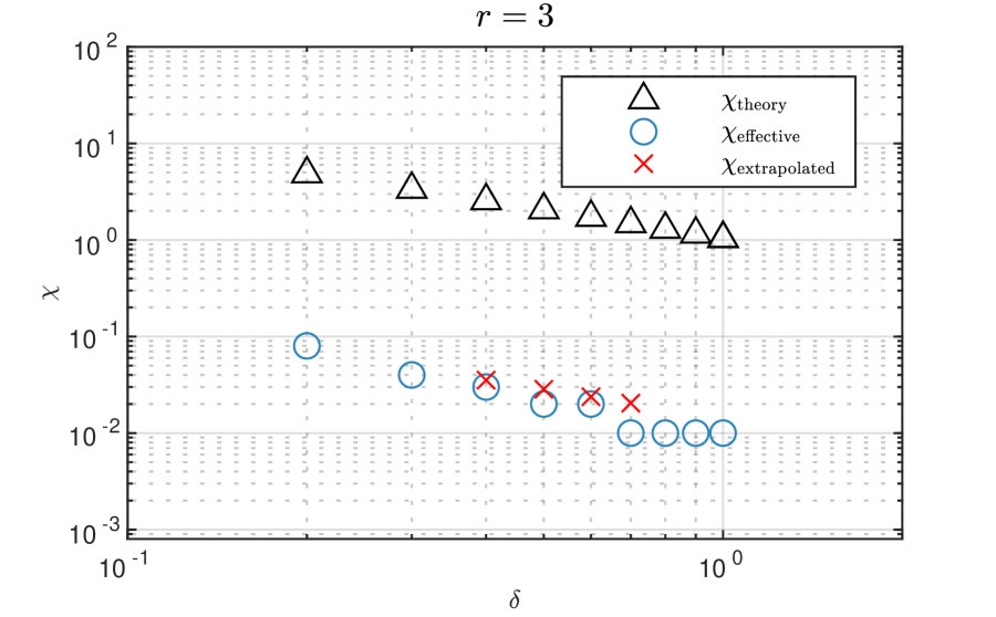
With and , the terms , , , , , and are relatively small. Therefore, (69) holds. Next, we investigate whether the scaling of with respect to the filter radius, , follows the scaling in (69) for .
In Fig. 5, the behavior of in (69) and with respect to the filter radius, , is shown for . The results for are similar. is found by solving the TR-ROM for different parameter values. Specifically, for each value, we consider values from . For each value, values from are considered, and is selected from the values.
Similar to the 2D flow past a cylinder problem, the results show that scales like a constant for certain for all considered values, where varies with the value. The linear regression in the figure indicates that, for certain , scales like for , and scales like for . Similar scalings are observed in and cases. In addition, for , the filtering is too aggressive such that . Therefore, the relaxation term is dominated by the unfiltered solution, . Hence, we see that does not change for .
Next, we use two values to estimate the ratio between and (69), and demonstrate that this ratio can be used with to predict at other values. To this end, we compute the ratio between and at and , and take the average of the two ratios. The extrapolated values at are then computed using and the average of the two ratios calculated above. From the results shown in Fig. 6, the extrapolated is close to , which highlights the predictive capabilities of the theoretical parameter scalings for in (69).
4.3.3 Scaling of with respect to
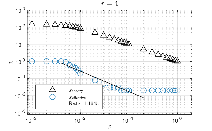
We also investigate the scaling of with respect to the number of modes, . First, we note that since for (compare columns 7 and 10 in Table 2) and , which does not depend on , the in (69) can be further simplified to
| (74) |
We consider two types of filter radius for studying the scaling of with respect to . First, we consider a constant filter radius, which is independent of . In this case, could scale like , a constant related to , or , depending on the value. That is, there exist two values, and , such that
| (75) | ||||
| (76) | ||||
| (77) |
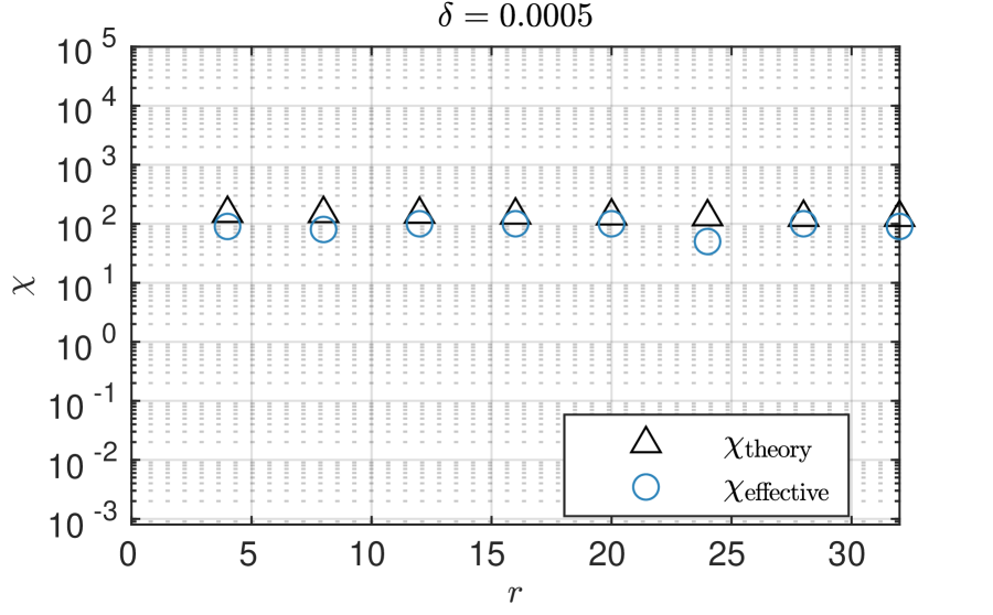
We study the scaling of with respect to for , , , and . In Fig. 7, the behavior of (74) and with respect to is shown for . For , scales like for the values considered. Although is a function of , its dependency on is weak. Therefore, behaves like a constant, as shown in the plot. We find that also scales like a constant with respect to . Specifically, is for almost all values, except for and . For , scales like a constant for the values considered. Although is not behaving like a constant, it fluctuates around . Similar behaviors are observed in and cases. We also note that at is much smaller compared to other values for all four values. A further investigation is required to gain a better understanding of this behavior.
The second type of filter we consider is the energy-based filter radius proposed in [22]:
| (78) |
is the characteristic length scale, and is the mesh size. We emphasize that, in contrast with the constant case, is a function of . Substituting (78) into (74), we find that is the largest term in the denominator for to . Hence, (74) indicates that should scale like for .
In Fig. 8, the behavior of in (74) and with respect to is shown. With the curve defined as , we clearly see that also scales like for the considered values, just like .
Next, we use four values to estimate the ratio between and (74), and demonstrate that this ratio can be used with to predict at other values. To this end, we compute the ratio between and at , and , and take the average of the four ratios. The extrapolated values at are then computed using and the average of the four ratio calculated above. From the results shown in Fig. 8, the extrapolated is close to for all values, except for . This highlights the predictive capabilities of the theoretical parameter scalings for in (74).
4.4 Parameter Scaling in the Predictive Regime
In this section, we investigate if, in the predictive regime, still scales like , given by the theoretical parameter scalings for in (74). We note that the quantity , which was used to determine in the reproduction regime (Sections 4.2–4.3), is in general sensitive because it is based on the instantaneous error. Hence, in the predictive regime, determined using could be sensitive to parameters and deteriorate the parameter scaling. Thus, is not a suitable metric for determining in the predictive regime. Therefore, to determine in both the reproduction and predictive regimes, we use an average metric, i.e., the error in the mean field, which is defined as
| (79) |
The model problem is the 2D lid-driven cavity at , but with a two times larger time interval, that is, . We consider a larger time interval compared to the previous examples so that the quantity is robust with respect to time.
In Fig. 9, the behavior of in the predictive regime with respect to the filter radius, , is shown for and , along with in (69) and in the reproduction regime. Similar results are obtained for and .
To determine in the reproduction regime, for each value, we simulate TR-ROM in the time interval with values from , and values from . For each value, in the reproduction regime is selected to be the largest value that yields similar accuracy (i.e., within ) as that of the optimal , which is defined to be the value that yields the smallest in the reproduction regime, with samples. To determine in the predictive regime, for each value, we consider the same parameter ranges for and as in the reproduction regime and simulate TR-ROM in a time interval , which is twice as large as the time interval in the reproduction regime. in the predictive regime is selected similarly, but with samples, where the last samples are the data in the predictive regime.
The results show that in the reproduction regime scales like for the range . More importantly, the results show that in the predictive regime also scales like in the same range as in the reproduction regime. In addition, for a given value, we observe that in the predictive regime has a similar magnitude as in the reproduction regime.
5 Conclusions
In this work, we performed the first numerical analysis of the recently introduced time-relaxation reduced order model (TR-ROM) [34]. Specifically, we proved unconditional stability in Lemma 3.1 and derived a priori error bounds in Theorem 3.1. In addition, in Section 3.1, we leveraged the a priori error bounds to derive a formula for the time-relaxation parameter, , which indicates the scaling of with respect to the reduced space dimension and filter radius . A key feature of our analysis is the coupling between the full order model (FOM) and the ROM, as our error bounds include terms related to the FOM discretization, which are critical for developing robust parameter scalings for the time-relaxation parameter, . In this study, we employed the spectral element method (SEM) as the FOM, making this the first time that error bounds for SEM-based ROMs have been proven.
In Section 4, we demonstrated that the error convergence rate in Theorem 3.1 and the time-relaxation parameter scalings with respect to (69) are recovered numerically in two test problems: the 2D flow past a cylinder and 2D lid-driven cavity. In addition, we estimated the ratio between the numerically found , denoted as , and at two values, and demonstrated that this ratio can be used with to predict at other values. Furthermore, for the 2D lid-driven cavity, we demonstrated that the scaling with respect to (74) is recovered numerically for both constant filter radius and energy-based filter radius [22]. Moreover, we showed that can be also used to predict at other values. In Section 4.4, we demonstrated that the scaling with respect in the reproduction regime is also observed in the predictive regime. In particular, we showed that in the predictive regime has a similar magnitude as in the reproduction regime for most values. This illustrates the practical value of the new parameter scaling.
For future work, there are several promising research directions to explore. These include performing numerical analysis (e.g., deriving a priori error bounds) for nonlinear filtering and data-driven extensions of the new TR-ROM and other regularized ROMs. These a priori error bounds could then be leveraged to determine new ROM parameter scalings. Finally, these scalings could be tested in the predictive regime of challenging numerical simulations (e.g., turbulent channel flow) to determine their range of applicability in practical settings.
6 Acknowledgments
This work was supported by the National Science Foundation through grants DMS-2012253 and CDS&E-MSS-1953113, and by grant PID2022-136550NB-I00 funded by MCIN/AEI/10.13039/ 501100011033 and the European Union ERDF A way of making Europe.
References
- [1] L. Berselli, T. Iliescu, W. Layton, Mathematics of Large Eddy Simulation of Turbulent Flows, Scientific Computation, Springer-Verlag, Berlin, 2006.
- [2] W. J. Layton, L. G. Rebholz, Approximate Deconvolution Models of Turbulence: Analysis, Phenomenology and Numerical Analysis, Vol. 2042, Springer Berlin Heidelberg, 2012.
- [3] S. Stolz, N. A. Adams, L. Kleiser, An approximate deconvolution model for large-eddy simulation with application to incompressible wall-bounded flows, Phys. Fluids 13 (4) (2001) 997–1015.
- [4] S. Stolz, N. A. Adams, L. Kleiser, The approximate deconvolution model for large-eddy simulations of compressible flows and its application to shock-turbulent-boundary-layer interaction, Phys. Fluids 13 (10) (2001) 2985–3001.
- [5] J. Belding, M. Neda, R. Lan, An efficient discretization for a family of time relaxation models, Comput. Methods Appl. Mech. Engrg. 391 (2022) 114510.
- [6] J. Belding, M. Neda, F. Pahlevani, Computational study of the time relaxation model with high order deconvolution operator, Results Appl. Math. 8 (2020) 100–111.
- [7] A. A. Dunca, M. Neda, Numerical analysis of a nonlinear time relaxation model of fluids, J. Math. Anal. Appl. 420 (2) (2014) 1095–1115.
- [8] V. J. Ervin, W. Layton, M. Neda, Numerical analysis of a higher order time relaxation model of fluids, Int. J. Numer. Anal. Model 4 (3) (2007) 648–670.
- [9] W. Layton, M. Neda, Truncation of scales by time relaxation, J. Math. Anal. Appl. 325 (2) (2007) 788–807.
- [10] M. Neda, X. Sun, L. Yu, Increasing accuracy and efficiency for regularized Navier-Stokes equations, Acta Appl. Math. 118 (2012) 57–79.
- [11] A. Takhirov, M. Neda, J. Waters, Modular nonlinear filter based time relaxation scheme for high Reynolds number flows, Int. J. Numer. Anal. Mod. 15 (2018-04-05) (2018) 699.
- [12] M. Neda, J. Waters, Finite element computations of time relaxation algorithm for flow ensembles, Appl. Eng. Lett 1 (2016) 51–56.
- [13] A. Takhirov, M. Neda, J. Waters, Time relaxation algorithm for flow ensembles, Num. Meth. P.D.E.s 32 (3) (2016) 757–777.
- [14] S. Breckling, M. Neda, T. Hill, A review of time relaxation methods, Fluids 2 (3) (2017) 40.
- [15] J. S. Hesthaven, G. Rozza, B. Stamm, Certified Reduced Basis Methods for Parametrized Partial Differential Equations, Springer, 2015.
- [16] A. Quarteroni, A. Manzoni, F. Negri, Reduced Basis Methods for Partial Differential Equations: An Introduction, Vol. 92, Springer, 2015.
- [17] P. Tsai, P. Fischer, E. Solomonik, Accelerating the Galerkin reduced-order model with the tensor decomposition for turbulent flows, arXiv preprint, http://arxiv.org/abs/2311.03694 (2023).
- [18] S. E. Ahmed, S. Pawar, O. San, A. Rasheed, T. Iliescu, B. R. Noack, On closures for reduced order models A spectrum of first-principle to machine-learned avenues, Phys. Fluids 33 (9) (2021) 091301.
- [19] L. Fick, Y. Maday, A. T. Patera, T. Taddei, A stabilized POD model for turbulent flows over a range of Reynolds numbers: Optimal parameter sampling and constrained projection, J. Comp. Phys. 371 (2018) 214–243.
- [20] K. Kaneko, P. Fischer, Augmented reduced order models for turbulence, Front. Phys. (2022) 808.
- [21] K. Kaneko, P.-H. Tsai, P. Fischer, Towards model order reduction for fluid-thermal analysis, Nucl. Eng. Des. 370 (2020) 110866.
- [22] C. Mou, E. Merzari, O. San, T. Iliescu, An energy-based lengthscale for reduced order models of turbulent flows, Nucl. Eng. Des. 412 (2023) 112454.
- [23] E. J. Parish, M. Yano, I. Tezaur, T. Iliescu, Residual-based stabilized reduced-order models of the transient convection-diffusion-reaction equation obtained through discrete and continuous projection, Arch. Comput. Methods Eng.To appear (2024).
- [24] V. John, Large Eddy Simulation of Turbulent Incompressible Flows, Vol. 34 of Lecture Notes in Computational Science and Engineering, Springer-Verlag, Berlin, 2004, Analytical and Numerical Results for a Class of LES Models.
- [25] T. C. Rebollo, R. Lewandowski, Mathematical and Numerical Foundations of Turbulence Models and Applications, Springer, 2014.
- [26] H. G. Roos, M. Stynes, L. Tobiska, Robust Numerical Methods for Singularly Perturbed Differential Equations: Convection-Diffusion-Reaction and Flow Problems., 2nd Edition, Vol. 24 of Springer Series in Computational Mathematics, Springer, 2008.
- [27] S. Giere, T. Iliescu, V. John, D. Wells, SUPG reduced order models for convection-dominated convection-diffusion-reaction equations, Comput. Methods Appl. Mech. Engrg. 289 (2015) 454–474.
- [28] J. Novo, S. Rubino, Error analysis of proper orthogonal decomposition stabilized methods for incompressible flows, SIAM J. Numer. Anal. 59 (1) (2021) 334–369.
- [29] M. Gunzburger, T. Iliescu, M. Schneier, A Leray regularized ensemble-proper orthogonal decomposition method for parameterized convection-dominated flows, IMA J. Numer. Anal. 40 (2) (2020) 886–913.
- [30] T. Iliescu, Z. Wang, Variational multiscale proper orthogonal decomposition: Convection-dominated convection-diffusion-reaction equations, Math. Comput. 82 (283) (2013) 1357–1378.
- [31] T. Iliescu, Z. Wang, Variational multiscale proper orthogonal decomposition: Navier-Stokes equations, Num. Meth. P.D.E.s 30 (2) (2014) 641–663.
- [32] V. John, B. Moreau, J. Novo, Error analysis of a SUPG-stabilized POD-ROM method for convection-diffusion-reaction equations, Comput. Math. Appl. 122 (2022) 48–60.
- [33] X. Xie, D. Wells, Z. Wang, T. Iliescu, Numerical analysis of the Leray reduced order model, J. Comput. Appl. Math. 328 (2018) 12–29.
- [34] P.-H. Tsai, P. Fischer, T. Iliescu, A time-relaxation reduced order model for the turbulent channel flow, J. Comput. Phys.To appear (2024).
- [35] P. Fischer, J. Kruse, J. Mullen, H. Tufo, J. Lottes, S. Kerkemeier, Nek5000–open source spectral element CFD solver, Argonne National Laboratory, Mathematics and Computer Science Division, Argonne, IL, https://nek5000.mcs.anl.gov/index.php/MainPage (2008).
- [36] Y. Maday, A. T. Patera, Spectral element methods for the incompressible Navier-Stokes equations, State-of-the-art surveys on computational mechanics (A90-47176 21-64). New York (1989) 71–143.
- [37] F. Ben Belgacem, C. Bernardi, N. Chorfi, Y. Maday, Inf-sup conditions for the mortar spectral element discretization of the Stokes problem, Numer. Math. 85 (2) (2000) 257–281.
- [38] C. Bernardi, Y. Maday, Uniform inf-sup conditions for the spectral discretization of the Stokes problem, Math. Models Methods Appl. Sci. 9 (3) (1999) 395–414.
- [39] W. Layton, Introduction to Finite Element Methods for Incompressible, Viscous Flows, SIAM publications, 2008.
- [40] R. Temam, Navier-Stokes Equations: Theory and Numerical Analysis, Vol. 2, American Mathematical Society, 2001.
- [41] J. G. Heywood, R. Rannacher, Finite-element approximation of the nonstationary Navier-Stokes problem. Part IV: Error analysis for second-order time discretization, SIAM J. Numer. Anal. 27 (2) (1990) 353–384.
- [42] J. de Frutos, J. Novo, A spectral element method for the Navier-Stokes equations with improved accuracy, SIAM J. Numer. Anal. 38 (3) (2000) 799–819.
- [43] P. Fischer, M. Schmitt, A. Tomboulides, Recent developments in spectral element simulations of moving-domain problems, in: Recent Progress and Modern Challenges in Applied Mathematics, Modeling and Computational Science, Springer, 2017, pp. 213–244.
- [44] G. Berkooz, P. Holmes, J. Lumley, The proper orthogonal decomposition in the analysis of turbulent flows, Ann. Rev. Fluid Mech. 25 (1) (1993) 539–575.
- [45] S. Volkwein, Proper Orthogonal Decomposition: Theory and Reduced-Order Modelling, Lecture Notes, University of Konstanzhttp://www.math.uni-konstanz.de/numerik/personen/volkwein/teaching/POD-Book.pdf (2013).
- [46] P. Tsai, P. Fischer, Parametric model-order-reduction development for unsteady convection, Front. Phys. 10 (2022) 903169.
- [47] P. Holmes, J. L. Lumley, G. Berkooz, Turbulence, Coherent Structures, Dynamical Systems and Symmetry, Cambridge, 1996.
- [48] K. Kunisch, S. Volkwein, Galerkin proper orthogonal decomposition methods for parabolic problems, Numer. Math. 90 (1) (2001) 117–148.
- [49] T. Iliescu, Z. Wang, Are the snapshot difference quotients needed in the proper orthogonal decomposition?, SIAM J. Sci. Comput. 36 (3) (2014) A1221–A1250.
- [50] I. Moore, A. Sanfilippo, F. Balarin, T. Iliescu, A priori error bounds for the approximate deconvolution Leray reduced order model, arXiv preprint, http://arxiv.org/abs/2410.02673 (2024).
- [51] B. Koc, S. Rubino, M. Schneier, J. R. Singler, T. Iliescu, On optimal pointwise in time error bounds and difference quotients for the proper orthogonal decomposition, SIAM J. Numer. Anal. 59 (4) (2021) 2163–2196.
- [52] S. L. Eskew, J. R. Singler, A new approach to proper orthogonal decomposition with difference quotients, Adv. Comput. Math. 49 (2) (2023) 33.
- [53] B. García-Archilla, V. John, J. Novo, Second order error bounds for POD-ROM methods based on first order divided differences, Appl. Math. Lett. 146 (2023) 108836.
- [54] B. García-Archilla, J. Novo, Pointwise error bounds in POD methods without difference quotients, arXiv preprint, http://arxiv.org/abs/2407.17159 (2024).
- [55] M. Germano, Differential filters of elliptic type, Phys. Fluids 29 (6) (1986) 1757–1758.
- [56] P. Grisvard, Elliptic Problems in Nonsmooth Domains, SIAM, 2011.
- [57] S. Kaya, C. C. Manica, Convergence analysis of the finite element method for a fundamental model in turbulence, Math. Models Methods Appl. Sci. 22 (11) (2012) 1250033.
- [58] J. Connors, Convergence analysis and computational testing of the finite element discretization of the Navier–Stokes alpha model, Num. Meth. P.D.E.s 26 (6) (2010) 1328–1350.
- [59] C. C. Manica, M. Neda, M. Olshanskii, L. G. Rebholz, Enabling numerical accuracy of Navier-Stokes- through deconvolution and enhanced stability, ESAIM Math. Model. Numer. Anal. 45 (2) (2011) 277–307.
- [60] A. A. Dunca, M. Neda, L. G. Rebholz, A mathematical and numerical study of a filtering-based multiscale fluid model with nonlinear eddy viscosity, Comput. Math. Appl. 66 (6) (2013) 917–933.
- [61] S. C. Huang, A. Johnson, M. Neda, J. Reyes, H. Tehrani, A generalization of the Smagorinsky model, Appl. Math. Comput. 469 (2024) 128545.
- [62] S. Ingimarson, M. Neda, L. Rebholz, J. Reyes, A. Vu, Improved long time accuracy for projection methods for Navier-Stokes equations using EMAC formulation, Int. J. Numer. Anal. Mod. 20 (2) (2023) 176–198.
- [63] V. J. Ervin, W. J. Layton, M. Neda, Numerical analysis of filter-based stabilization for evolution equations, SIAM J. Numer. Anal. 50 (5) (2012) 2307–2335.
- [64] K. Kaneko, P. Tsai, P. Fischer, NekROM, https://github.com/Nek5000/NekROM.