HETDEX-LOFAR Spectroscopic Redshift Catalog ¹¹1Based on observations obtained with the Hobby-Eberly Telescope, which is a joint project of the University of Texas at Austin, the Pennsylvania State University, Ludwig-Maximilians-Universität München, and Georg-August-Universität Göttingen.

Maya H. Debski Department of Astronomy, The University of Texas at Austin, 2515 Speedway Boulevard, Austin, TX 78712, USA Gregory R. Zeimann Hobby Eberly Telescope, University of Texas at Austin, 2515 Speedway Boulevard, Austin, TX, 78712, USA McDonald Observatory, The University of Texas at Austin, 2515 Speedway Boulevard, Austin, TX 78712, USA Gary J. Hill Department of Astronomy, The University of Texas at Austin, 2515 Speedway Boulevard, Austin, TX 78712, USA McDonald Observatory, The University of Texas at Austin, 2515 Speedway Boulevard, Austin, TX 78712, USA Donald P. Schneider Department of Astronomy & Astrophysics, The Pennsylvania State University, University Park, PA 16802, USA Institute for Gravitation and the Cosmos, The Pennsylvania State University, University Park, PA 16802, USA Leah Morabito Centre for Extragalactic Astronomy, Department of Physics, Durham University, South Road, Durham DH1 3LE, UK Institute for Computational Cosmology, Department of Physics, Durham University, South Road, Durham DH1 3LE, UK Gavin Dalton Oxford Astrophysics, University of Oxford, Keble Road, Oxford OX1 3RH, UK RALSpace, STFC Rutherford Appleton Laboratory, Didcot, OX11 0QX, UK Matt J. Jarvis Oxford Astrophysics, University of Oxford, Keble Road, Oxford OX1 3RH, UK Erin Mentuch Cooper Department of Astronomy, The University of Texas at Austin, 2515 Speedway Boulevard, Austin, TX 78712, USA McDonald Observatory, The University of Texas at Austin, 2515 Speedway Boulevard, Austin, TX 78712, USA Robin Ciardullo Department of Astronomy & Astrophysics, The Pennsylvania State University, University Park, PA 16802, USA Institute for Gravitation and the Cosmos, The Pennsylvania State University, University Park, PA 16802, USA Eric Gawiser Department of Physics and Astronomy, Rutgers, the State University of New Jersey, Piscataway, NJ 08854, USA Nika Jurlin Department of Astronomy, The University of Texas at Austin, 2515 Speedway Boulevard, Austin, TX 78712, USA

Abstract

We combine the power of blind integral field spectroscopy from the Hobby-Eberly Telescope (HET) Dark Energy Experiment (HETDEX) with sources detected by the Low Frequency Array (LOFAR) to construct the HETDEX-LOFAR Spectroscopic Redshift Catalog. Starting from the first data release of the LOFAR Two-metre Sky Survey (LoTSS), including a value-added catalog with photometric redshifts, we extracted 28,705 HETDEX spectra. Using an automatic classifying algorithm, we assigned each object a star, galaxy, or quasar label along with a velocity/redshift, with supplemental classifications coming from the continuum and emission line catalogs of the internal, fourth data release from HETDEX (HDR4). We measured 9,087 new redshifts; in combination with the value-added catalog, our final spectroscopic redshift sample is 9,710 sources. This new catalog contains the highest substantial fraction of LOFAR galaxies with spectroscopic redshift information; it improves archival spectroscopic redshifts, and facilitates research to determine the [O II] emission properties of radio galaxies from $0.0<z<0.5$ , and the Ly $\alpha$ emission characteristics of both radio galaxies and quasars from $1.9<z<3.5$ . Additionally, by combining the unique properties of LOFAR and HETDEX, we are able to measure star formation rates (SFR) and stellar masses. Using the Visible Integral-field Replicable Unit Spectrograph (VIRUS), we measure the emission lines of [O III], [Ne III], and [O II] and evaluate line-ratio diagnostics to determine whether the emission from these galaxies is dominated by AGN or star formation and fit a new SFR-L_150MHz relationship.

1 Introduction

For several decades, extragalactic radio surveys were a powerful probe of the distant Universe. In fact, until the mid-1990s, they served as an effective method for finding high redshift galaxies through optical identification of ultra steep radio sources, a poorly understood type of diffuse radio source characterized by power law spectra (e.g., Slee et al., 2001; Feretti et al., 2012; Whyley et al., 2024). Recent radio surveys have reached sub-milliJansky flux density levels, providing the framework to make these surveys a means of identifying star-forming galaxies. Previous studies have demonstrated a tight correlation between low-frequency radio continuum, which is dominated by synchrotron emission of relativistic electrons produced by supernovae, and the far-infrared (FIR) flux of galaxies (e.g., Yun et al., 2001). FIR emission is an established strong indicator of star formation rate (SFR) (Yun et al., 2001), thereby legitimizing the idea that radio continuum can act as a tracer of SFR (e.g., Condon et al., 2002; Pannella et al., 2009; Heesen et al., 2014; Davies et al., 2017; Smith et al., 2021).

Radio surveys have played a small part in investigating star formation history, as they are generally limited by their sensitivity; however, star forming galaxies become increasingly important at fainter flux densities and totally dominate the source counts below $\simeq$ 0.1 mJy at 1.4 GHz (e.g., Padovani et al., 2011, 2015; Bonzini et al., 2013), opening the door for new, more sensitive radio surveys to push to the forefront of SFR investigations (De Zotti et al., 2019). In particular, the introduction of the Square Kilometer Array (SKA; Grainge et al., 2017) with its square kilometer collecting surface and large range of frequencies (between 50 MHz - 24 GHz) will extend the flux density limit more than three orders of magnitude. The science of the SKA will be used to explore areas such as strong-field tests with pulsars and black holes, cosmic dawn and the epoch of reionization, cosmology and dark energy, the origin and evolution of cosmic magnetism, galaxy evolution probed by neutral hydrogen, the cradle of life and astrobiology, and galaxy and cluster evolution (De Zotti et al., 2019). To prepare for this new era of radio surveys, SKA will work alongside Pathfinders, like the International Low-frequency Array (LOFAR) Telescope (ILT), to contribute scientific and technical developments for direct use by SKA.

The combination of multiple massive surveys at different wavelengths enables scientific projects otherwise unachievable (e.g., Smith et al., 2016; Williams et al., 2019). The LOFAR Two-metre Sky Survey (LoTSS) is a sensitive, high-resolution (120-168 MHz, centered at 150 MHz) survey that has already collected millions of sources and is advancing our understanding of the formation and growth of massive black holes (e.g., Best et al., 2014; Mingo et al., 2019, 2022; Yue et al., 2023; Sabater et al., 2019), the evolution of galaxy clusters (e.g., Venemans et al., 2007; Wylezalek et al., 2013; Timmerman et al., 2022, 2024; Botteon et al., 2020), and the properties of high redshift radio sources (e.g., Gloudemans et al., 2021; Cordun et al., 2023). However, many of these scientific forefronts require optical counterparts for multi-wavelength matching as well as a robust set of distances or redshifts.

HETDEX (Gebhardt et al., 2021; Hill et al., 2021) is blind-spectroscopic survey conducted with the wide-field upgraded Hobby Eberly Telescope (Ramsey et al., 1998; Hill et al., 2021) using the Visible Integral Field Replicable Unit Spectrograph (VIRUS; Hill et al., 2021).²²2VIRUS is a joint project of the University of Texas at Austin, Leibniz-Institut für Astrophysik Potsdam (AIP), Texas A&M University (TAMU), Max-Planck-Institut für Extraterrestriche-Physik (MPE), Ludwig-Maximilians-Universität München, Pennsylvania State University, Institut für Astrophysik Göttingen, University of Oxford, Max-Planck-Institut für Astrophysik (MPA), and The University of Tokyo. HETDEX aims to measure the expansion history of the Universe at $z\simeq 2.5$ by detecting and mapping the spatial distribution of about a million Ly $\alpha$ emitting galaxies (LAEs). The redshift range for LAE detection is $1.9<z<3.5$ over a total of $\sim 540$ deg² (11 Gpc³ comoving volume) including $\sim 400$ deg² in the HETDEX Spring field. The internal data release 4 includes 67.48 deg² of spectroscopic observations in the Spring Field with wavelengths spanning 3470-5540 Å. This amounts to 523 million fiber spectra. In the LOFAR/HETDEX overlap region, we aim to produce a new, large spectroscopic radio-source catalog that would facilitate breakthroughs in the study of galaxy proto-clusters, emission line properties of radio galaxies, and even radio-loud stars.

The combination of wide-field photometric surveys for spectral energy distribution information and optical spectroscopic follow-up from HETDEX/VIRUS offers a characterization of key physical parameters, the most important of which being distance as represented by spectroscopic redshift (e.g., SDSS; Almeida et al., 2023). The combination of HETDEX and LOFAR will also allow the measurement of SFR, and stellar mass because of the VIRUS sensitivity. Both the LOFAR radio selection and HETDEX optical spectroscopic identifications are sensitive to SFR and AGN activity. Using VIRUS, we can measure the emission lines of [O III], H $\beta$ , [Ne III], and [O II]. Emission line diagnostics like those of [O III]/H $\beta$ , [Ne III]/[O II], R₂₃, and [O III]/[O II] can provide information on a system’s metallicity and ionization parameter, and discriminate between excitation by AGN or star formation. Moreover, by comparing these line ratios as a function of stellar mass with those determined for galaxies found via selection methods, we can ultimately investigate how similar or dissimilar populations of galaxies are.

In $\S$ 2, we describe the observations, data sets, and tools required to identify HETDEX counterparts to LOFAR sources and analyze the objects $\S$ 3 focuses on the redshift analysis of the sample, including a description of the classification code Diagnose that was developed for the HET VIRUS Parallel Survey (HETVIPS) and its application in this catalog. We also describe the matching process for the sources within both the HETDEX survey and LoTSS, as well as the criteria for determining whether the matches were accurate. This section also features a broad overview of the redshift results alongside the overall catalog breakdown and selected results from the catalog. In addition, we examine star formation in a sub-sample of galaxies in $\S$ 4. Finally, we discuss possible scientific applications and uses for this data set in $\S$ 5. Throughout this work, we use flat $\Lambda$ CDM cosmological parameters $H_{0}=67.66$ km Mpc^-1 s^-1 and $\Omega_{m,0}=0.30966$ (Planck Collaboration et al., 2020).

2 Data and Observations

In this section, we present an overview of the LoTSS DR1 and the HDR4 data sets used in this work. This includes the value-added catalogs from previous efforts, the matching methodology, and the spectral extractions.

2.1 LOFAR Two-metre Sky Survey

The LOFAR Two-metre Sky Survey (LoTSS) is a high-resolution 120-168 MHz survey centered at 150 MHz, with a median sensitivity of $S_{\text{150MHz}}=71\mu\text{Jy}\ \rm beam^{-1}$ and a point-source completeness of 90% at an integrated flux density of 0.45 mJy (Shimwell et al., 2017). The spatial resolution of the images is 6″ and the astrometric accuracy of the data is within $0.2$ ″ (Shimwell et al., 2019). The first data release includes 424 deg² in the HETDEX Spring Field (RAs between 10 ${}^{\text{h}}$ 45 ${}^{\text{m}}$ and 15 ${}^{\text{h}}$ 30 ${}^{\text{m}}$ and DECs ranging from 45°00′to 57°00′). There are 325,694 sources in the first data release for the HETDEX Spring field. Additionally, the LoTSS DR1 provides the astrometric precision needed to identify optical and infrared counterparts. We use the first data release because it specifically targeted the HETDEX Spring field, and while LoTSS DR2 (formed by two regions centered at RA = 12h45m00s, DEC = +44^∘30^′00^′′ and RA = 1h00m00s, DEC = +28^∘00^′00^′′, spanning 4178 and 1457 deg² respectively) is available, it only expands upon the area of the first data release, essentially making DR1 and DR2 interchangeable for our purposes.

Williams et al. (2019) combined Pan-STARRS $grizy_{\rm P1}$ photometry (Chambers et al., 2016) with data from the Wide-field Infrared Survey Explorer (WISE; Wright et al., 2010) over the LoTSS DR1 region. Using a combination of statistical techniques and visual identification, Williams et al. (2019) constructed a color- and magnitude-dependent likelihood ratio method for statistical identification. This resulted in a value-added catalog³³3https://lofar-surveys.org/public/LOFAR_HBA_T1_DR1_merge_ID_optical_f_v1.2b_restframe.fits with 318,520 radio sources, of which 231,716 (73%) have optical and/or IR identifications in Pan-STARRS and WISE.

Along with optical/IR counterparts for each radio source, the LoTSS DR1 value-added catalog includes photometric redshift estimates from Duncan et al. (2019). These estimates are crucial for identifying properties of the radio sources, as SDSS provides spectroscopic redshifts for less than one percent (2,690) of the sources. In the near future, the William Herschel Telescope Enhanced Area Velocity Explorer (WEAVE; Dalton et al., 2012, 2014) multi-object and integral field spectrograph will measure redshifts of over a million LoTSS sources as part of the WEAVE-LOFAR survey (Smith et al., 2016). We can take the first step in informing that large effort by increasing the known spectroscopic redshifts by combining the LoTSS DR1 value-added catalog with the fourth data release from the HETDEX survey.

2.2 HETDEX Data Release 4

The HETDEX survey is designed to measure the Hubble expansion parameter and angular diameter distances by using the spatial distribution of nearly one million Ly $\alpha$ emitting galaxies. The survey employs the VIRUS instrument which is comprised of a set of 78 fiber integral field units (IFUs) feeding 156 identical spectrographs that produce 34,944 spectra covering the wavelength range 3470 Å – 5540 Å at a resolving power $R\approx 800$ . The IFUs are arrayed in a grid pattern on the sky with a fill factor that is $\simeq$ 1/4.5, covering 56 arcmin² within an 18′ diameter field. Each IFU covers a solid angle of approximately $51\arcsec\times 51\arcsec$ and feeds two spectrographs, each with 224 fibers. The individual fibers are $1\farcs 5$ in diameter and the spacing between the fiber centers is $2\farcs 2$ . During HETDEX observations, a dither pattern of three exposures nearly fills these gaps ( $\sim$ 94% sky coverage; see Hill et al. (2021) for details). The astrometric accuracy of the fiber positions for HETDEX is 0.35″(Gebhardt et al., 2021).

The HETDEX survey serves as the primary observing mode at the HET during dark sky conditions, accumulating a wealth of data. The internal fourth data release completed observations on 2023-08-31, and it includes $\sim$ 67.48 deg² of fiber sky coverage with exposures from August 2017 through August 2023. The majority of these observations are in the HETDEX Spring Field with 67.48 deg² sky coverage and 523 million fiber spectra. The data reductions are described in Gebhardt et al. (2021), but to summarize: the HETDEX team produced two main products — a full set of flux-calibrated fiber spectra and a catalog of automatically detected and classified sources (Mentuch Cooper et al., 2023).

To construct the source catalog the HETDEX team ran two object detection algorithms: one designed to find emission line sources and the other built to search for continuum emission (Mentuch Cooper et al., 2023). From these two raw catalogs, source sizes were defined using a friends of friends algorithm to avoid multiple detections of the same object. The team then took a multi-pronged approach to source classification and redshift assignment. The details of the classification and redshift assignment can be found in Mentuch Cooper et al. (2023). In short, each source was classified either as a star (STAR), a low redshift galaxy with no [O II] emission (LZG), an [O II] emitting galaxy (O II), a Ly $\alpha$ emitting galaxy (LAE), or an active galactic nuclei (AGN).

The HDR4 catalog is dominated by emission-line galaxies and includes 920,715 LAE candidates with $1.88<z<3.52$ and with a signal-to-noise greater than 4.8. Also included in the catalog are 451,224 [O II]-emitting galaxies at $z<0.5$ , 775,063 stars, 98,801 low-redshift ( $z<0.5$ ) galaxies without emission lines, and 48,194 AGN. The catalog provides sky coordinates, redshifts, line identifications, classification information, line fluxes, [O II] and Ly $\alpha$ line luminosities when applicable, and spectra for all identified sources processed by the HETDEX detection pipeline.

Although the catalog provides many of the products that we need, we can supplement the HETDEX effort by extracting spectra at the precise locations of the LoTSS sources, and then running similar classification tools for a complete redshift analysis of the combined catalogs.

2.2.1 HETDEX Spectral Extractions

We use the HETDEX-API⁴⁴4https://github.com/HETDEX/hetdex_api (Mentuch Cooper et al., 2023) to extract a spectrum for the 28,705 sources in the LoTSS DR1 catalog with fiber coverage in HDR4. For the 28,705 sources, we first collect all fiber spectra within a $3.5\arcsec$ radius. Using the seeing measured from the VIRUS data (see Gebhardt et al., 2021 for details), we construct a Moffat PSF model ( $\beta=3.5$ , Moffat 1969). At each wavelength, we shift our fiber locations following the differential atmospheric refraction models for the fixed-altitude HET and convolve the PSF with the VIRUS fibers. This calculates the fraction of the object’s light covered by each fiber. Using these fiber coverage values as weights, we normalize the weights to one, retaining the normalization value, and perform a weighted extraction using the Horne (1986) optimal extraction formula. Finally, the resultant spectrum is corrected to a total flux using the normalization value. Within a $3\farcs 5$ aperture, the total fiber coverage is between 90-95%.

Although a PSF spectral extraction is not a natural method for each source in the catalog, it provides a higher signal to noise methodology than simpler aperture extractions and only introduces a minimal chromatic flux response issue for extended sources. We are not immediately concerned with the absolute calibration of our spectral extractions as the primary goal is the determination of redshift. A more appropriate extraction can be done for individual science cases starting from the information driven by the description below.

The vast majority of our sample have an average continuum signal to noise (S/N) of less than two per 2 Å pixel in the wavelength window of 4670-4870Å. However, it is clear that if the S/N is greater than $\sim 4$ , a clear source classification and redshift measurement are possible by eye. Although the sample is not too large for visual analysis, automatic tools with repeatable and similar success rates are available for this purpose (e.g., Bolton et al., 2012).

3 Classifications and Redshifts

The methodology for our classification scheme begins with the spectral extractions at the sky positions of each LoTSS DR1 source. We use Diagnose (Debski & Zeimann, 2024), a spectral classification code developed for the HET VIRUS Parallel Survey (HETVIPS) catalog (Zeimann et al., 2024), to automatically classify each source and assign a redshift.

3.1 Diagnose

The Diagnose code assigns one of four classifications for each source (star, galaxy, quasar, or unknown) while returning a redshift estimate for the galaxies and quasars and a velocity estimate for the stars. Diagnose determines a spectral classification and redshift estimate for each source via a ${\chi}^{2}$ minimization for linear combinations of principal component templates. In particular, Diagnose uses a principal component analysis (PCA) with the templates of redrock⁵⁵5https://github.com/desihub/redrock-templates, which include 10 components for galaxies and four components for quasars. Stars are classified by type, with six components for B, A, F, G, K, M, and white dwarfs.

By convolving the high resolution templates of redrock to the $R\approx 800$ resolution of VIRUS, and then fitting these templates to the data using a range of redshifts, Diagnose computes three best-fit ${\chi}^{2}$ values: one for stellar type and velocity, one for galaxy type and redshift, and one for a quasar and redshift. Diagnose then compares the best fit of these three ${\chi}_{\nu}^{2}$ values to the second best fit and evaluates the difference against a statistical threshold. If this difference is larger than a statistical threshold, the source is classified as the best fit template (i.e., star, galaxy, or quasar). If the difference is not larger than the threshold, the source is classified as unknown. Using Diagnose, the HETDEX-LOFAR Spectroscopic Redshift Catalog is able to produce classifications and redshift estimates for sources within LoTSS with no known spectroscopic redshifts.

The power of Diagnose is in identifying strong features, usually in the continuum. As the sources become fainter with lower signal to noise in the continuum, Diagnose becomes less effective and often returns an a unknown label. However, many of the radio sources in the HETDEX-LOFAR catalog have strong emission features but weak continua. For these sources, we can use the HDR4 catalog to both check our initial Diagnose classifications and supplement our identifications.

3.2 LoTSS-HDR4 Catalog Matching

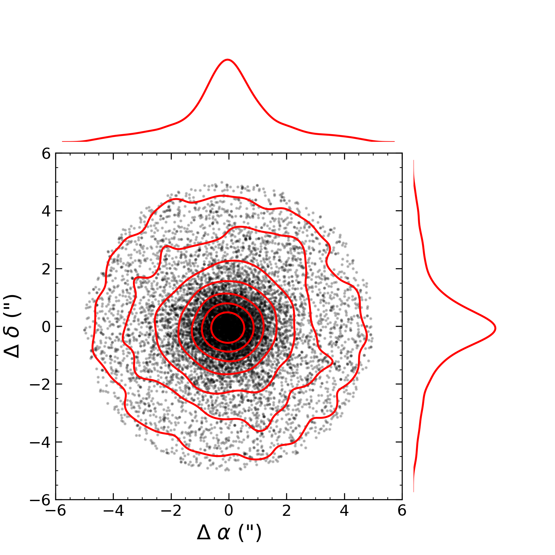
Refer to caption — Figure 1: Comparison between $\Delta\alpha$ and $\Delta\delta$ at initial matching radius of 5″for the 7,409 matches found between the HETDEX HDR4 catalog and the LoTSS sources. The x-axis represent the $\Delta\alpha$ and the y-axis represents the $\Delta\delta$ . Sources within a radius of 2″have less than 5.43% chance of being false matches when fitted with a uniform + Gaussian distribution model.

To match the LoTSS data set to sources in the HDR4 catalog, we use the HETDEX-API, including the ElixerWidget (Davis et al., 2023). We began by using an initial matching radius of 5″ to find counterparts for the 28,705 LoTSS sources. Given the astrometric uncertainty of the two catalogs, this should be a more than ample starting threshold. We found 7,409 matches and plot the $\Delta$ RA vs. $\Delta$ Dec in Fig 1. We fit a 2D uniform + Gaussian distribution model in $\Delta$ RA and $\Delta$ Dec space to determine the matching standard deviation and estimate the spurious match fraction. We found a standard deviation of $0.61$ ″ in $\Delta$ RA and $0.65$ ″ in $\Delta$ Dec. Thus, we use a final matching radius of 2″ which is roughly 3 times the standard deviation. For a matching radius of 2″ we estimate that only $\sim$ 5% of the counterparts are spurious by subtracting the area under the Gaussian distribution model from the area under the 2D uniform distribution model and dividing by the area under the 2D uniform distribution model.

3.3 Combining Diagnose and HDR4

Here we describe how we combine our Diagnose classifications/redshifts with the classifications/redshifts obtained from the LoTSS-HETDEX catalog matching. Starting from the 28,705 radio sources, Diagnose confidently identified 6,480 objects as a star, galaxy, or quasar; The remaining 21,081 sources did not have a reliable classification. Of those, 998 objects had insufficient spectral coverage for either a Diagnose or a catalog label; this is due to masking of bad fibers/amplifiers in the dataset after the initial spatial matching.

For the 7,409 spatial matches between LoTSS-HETDEX catalog, we collected the classification and redshift from HDR4. When comparing the sources with both a Diagnose and HDR4 redshift, we find good agreement, with 92.3% of the objects agreeing to within $\Delta$ z = 0.05. This is not entirely surprising as the HDR4 classification scheme uses Diagnose for sources with continuum $g$ -band magnitudes brighter than 22. For the objects with discrepant redshifts, the most common reason was Diagnose labeling an emission line as [O II], rather than Ly $\alpha$ . This occurred 3.03% of the time. As noted before, we also expect a $\sim$ 5% spurious match fraction between HDR4 and LoTSS, which may account for the remaining disagreement between the two redshift estimates.

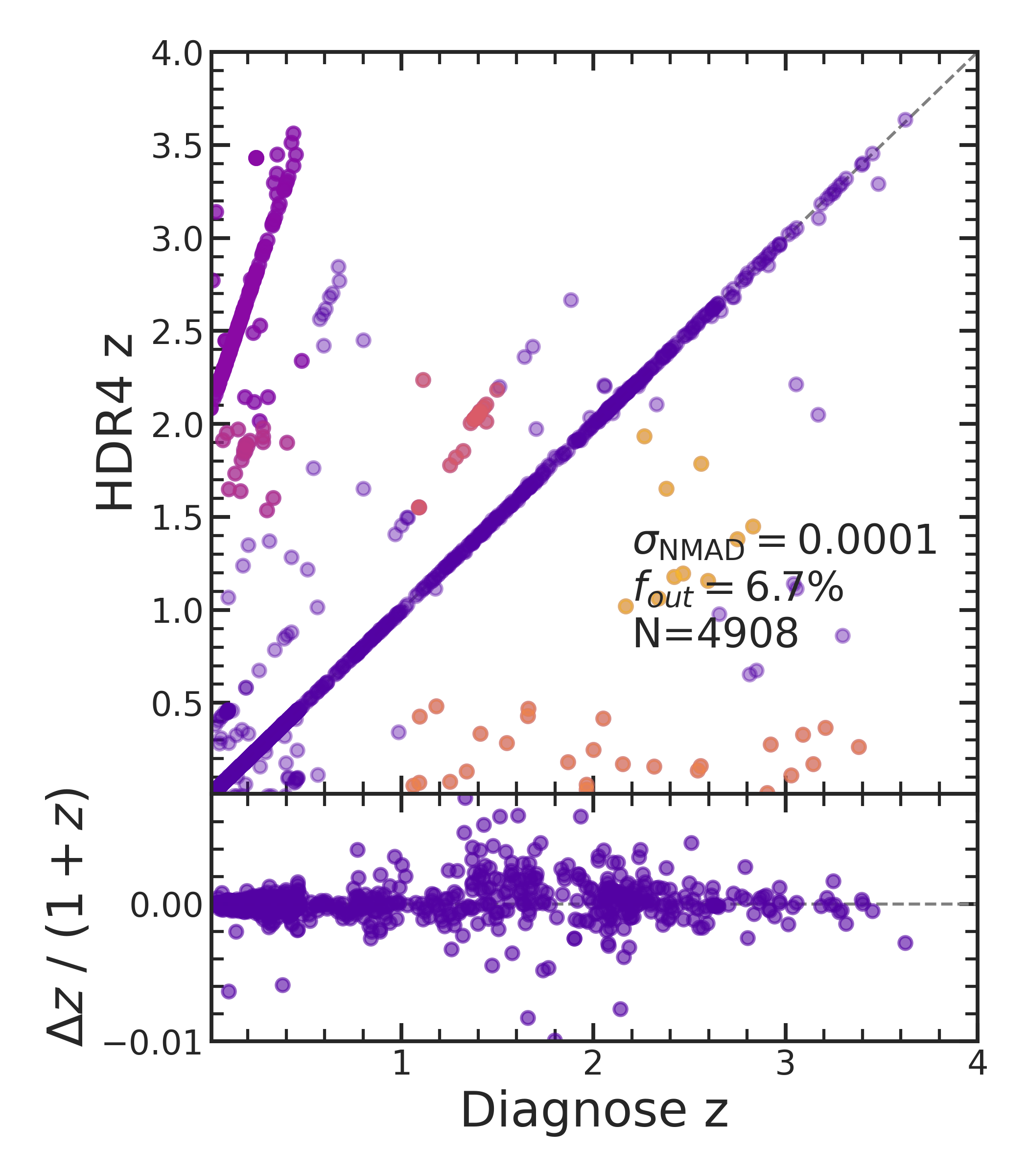
Comparing the HDR4 spectroscopic redshifts with our Diagnose redshifts, we find 4,908 sources in common. Figure 2 compares the two redshifts; the outlier fraction is 6.7%, while the standard deviation of the remaining objects is ${\sigma}_{z}=0.0001$ . Figure 2 also highlights groups of particular interest within the set of objects with discrepant redshifts. For each of these groups, we investigated the spectra by eye and determined criteria for determining which redshift is the best fit. These criteria and the process for choosing the best redshift are detailed in Appendix A. After applying all of the criteria to the different groups of spurious matches, the outlier fraction reduces from 6.7% to 2.3%.

3.4 LoTSS DR1 Value-Added Catalog Redshifts

Within 28,705 LoTSS sources, there are 11,807 objects with photometric redshifts and 2,690 sources with spectroscopic redshifts in the value-added catalog from Williams et al. (2019) and Duncan et al. (2019). The majority of spectroscopic redshifts were compiled from the Sloan Digital Sky Survey (SDSS) Data Release 14 (DR14; Abolfathi et al., 2018). These redshifts were supplemented by additional spectroscopic data from a range of deep optical surveys in the literature, mostly covering the Extended Groth Strip within the HETDEX Spring field. We refer to the spectroscopic redshifts in the value-added catalog as archival redshifts.

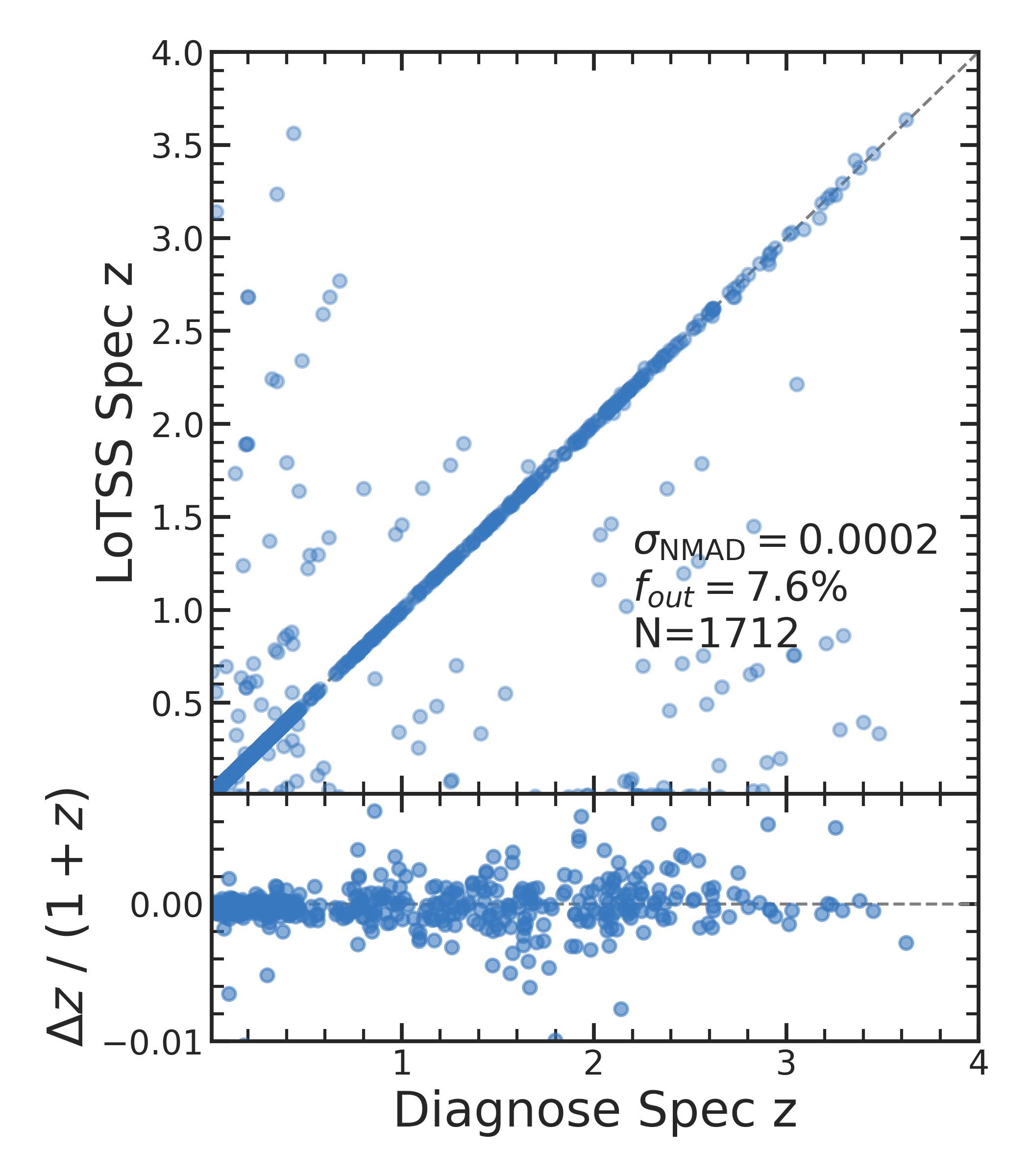
Comparing the archival spectroscopic redshifts with our HETDEX-LOFAR catalog we find 1,701 sources in common. The vast majority ( $\sim$ 75%) of the archival redshifts that are not in our catalog are in the redshift desert of VIRUS (0.5 $<$ z $<$ 1.9) where there are no strong emission lines. Investigating the overlapping sources, we find good agreement between our spectroscopic redshifts and those in the literature. Figure 3 shows the outlier fraction is 7.6% with a standard deviation of non-outlying sources is ${\sigma}_{z}=0.0002$ .

We also compared our spectroscopic redshifts to the photometric estimates from the LoTSS value-added catalog. Figure 4 shows this comparison over the range $0.0<z<0.5$ ; we find a good agreement between the two measurements with ${\sigma}_{z}=0.0614$ .

3.5 Classification and Redshift Methodology

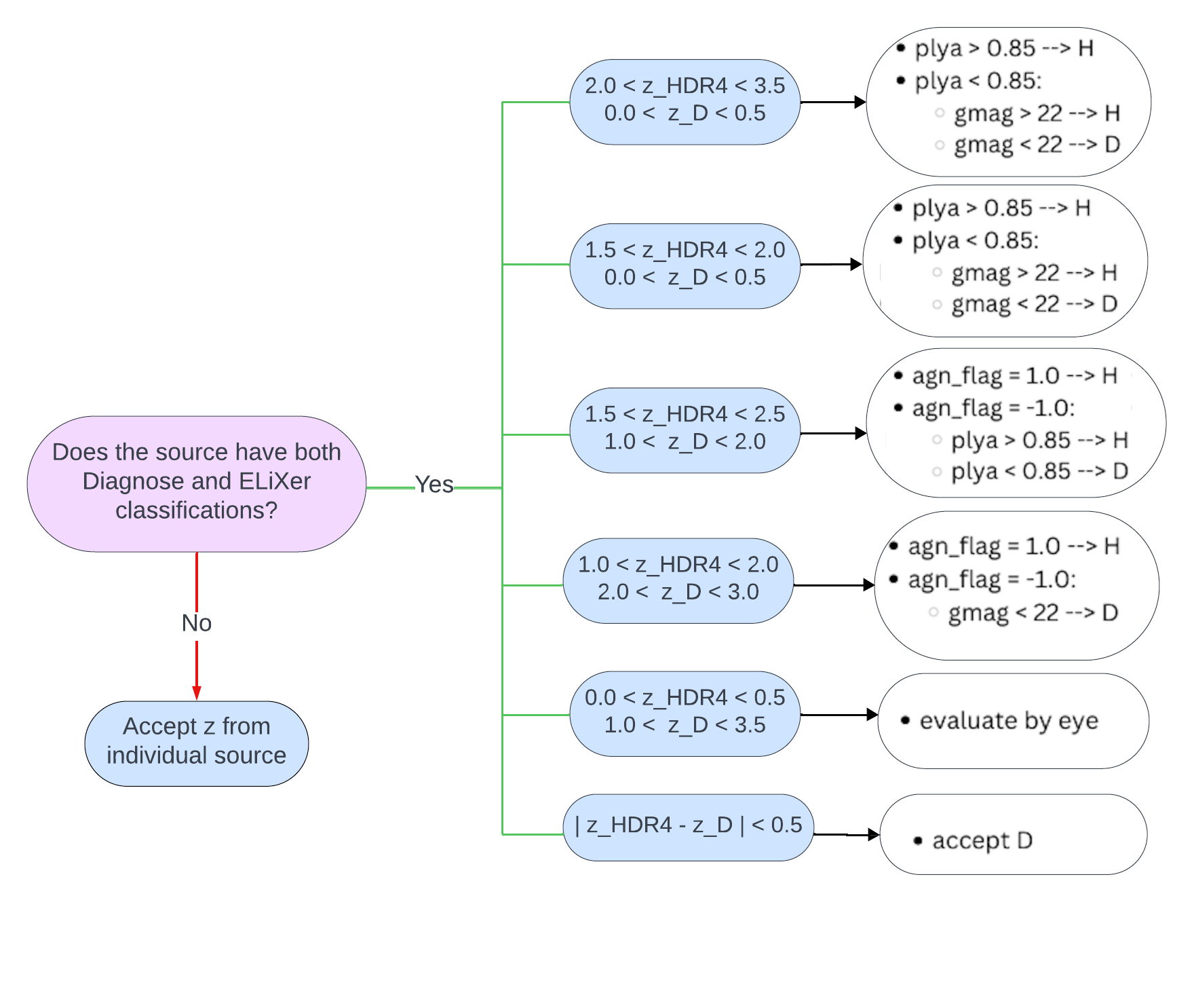
The HETDEX-LOFAR spectroscopic redshifts and classifications have three origins: Diagnose, HDR4, and archival. We discussed the combination of Diagnose and HDR4 redshifts in §3.3, and with all three origins we follow a similar logic. If Diagnose has a robust redshift, this is used. If not and HDR4 has a redshift, then this is used. Finally, if neither Diagnose nor HDR4 provide a redshift for the source, but the value-added catalog does then we use the archival spectroscopic redshift. We prioritize archival redshifts last in order to maximize the number of new redshifts determined for this catalog. Figure 5 shows the final redshift distribution for the 9,710 sources and the origin of the redshift. The overall detection and classification pipeline is outlined in Figure 6.

Our classification follows mostly from the redshift of the source and the origin catalog. We group all sources labeled ‘STAR’ by Diagnose or HDR4 together as ‘STAR’. We group all objects labeled ‘QSO’ or ‘AGN’ in Diagnose or HDR4, respectively, as ‘AGN’; this is done for all redshifts $0.0<z<3.5$ . Classifications of ‘LZG’ and ‘OII’ from HDR4 and ‘GALAXY’ from Diagnose are all grouped under the label ‘LOWZGAL’ for galaxies $0.0<z<0.5$ . Classifications of ‘LAE’ from HDR4 are grouped as ‘HIGHZGAL’ for systems with $1.9<z<3.5$ . Finally, if the redshift comes from the archive, we label the group ‘ARCHIVE’ with $0.0<z<3.5$ . So our final five labels are ‘STAR’, ‘AGN’, ‘LOWZGAL’, ‘HIGHZGAL’, and ‘ARCHIVE’. Table 1 includes a breakdown of the number of sources at different steps of the classification process, including the final catalog size.

Number of Sources	Description
325,694	Sources in LoTSS DR1
28,705	Spectral matches between LoTSS DR1 & HETDEX DR4
4,908	Sources w/ Diagnose & ELiXer redshifts
9,710	# of spectroscopic redshifts in final HETDEX-LOFAR catalog
9,087	New spectroscopic redshifts in final catalog
197	‘STAR’ in final catalog
804	‘AGN’ in final catalog
6,394	‘LOWZGAL’ in final catalog
1,075	‘HIGHZGAL’ in final catalog
757	‘ARCHIVE’ in final catalog

Table 1: Breakdown of the number of sources relevant to different steps of the classification and redshift assignment pipeline including final spectroscopic redshift catalog size.

3.6 HETDEX-LOFAR Spectroscopic Catalog

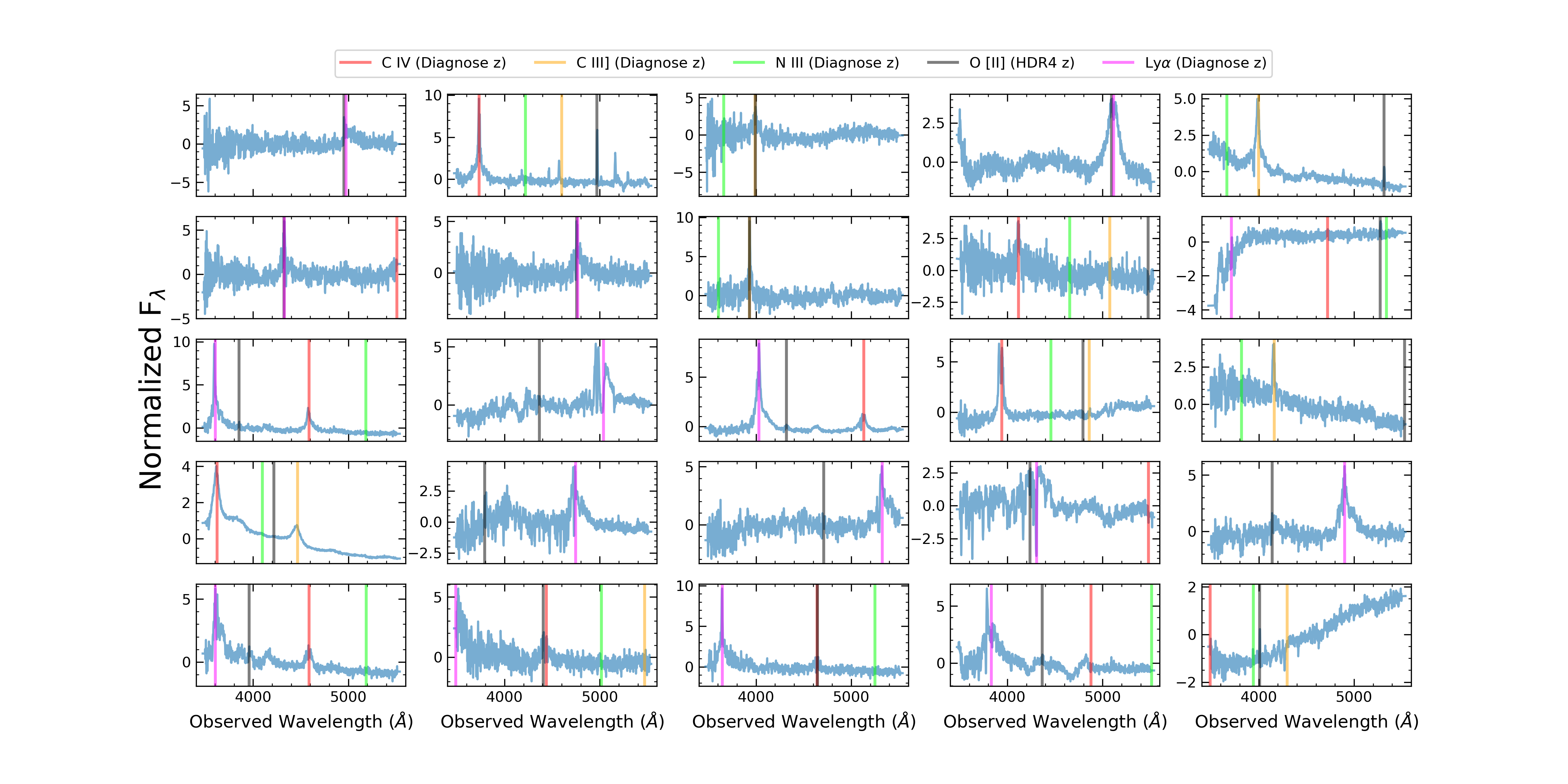
Our final compiled spectroscopic redshift catalog includes 9,710 total redshifts: 197 ‘STAR’, 804 ‘AGN’, 6,394 ‘LOWZGAL’, 1,075 ‘HIGHZGAL’, and 757 ‘ARCHIVE’. Table 2 explains the column names for the final catalog. In Figure 7, we show three example spectra for each of the five labels.

Column Name	Description	Data Type
objID	LoTSS Object ID	string
source_name	Source Name	string
RA	PanSTARRS1 Right Ascension (J2000)	float
Dec	PanSTARRS1 Declination (J2000)	float
z_diagnose	Best fit redshift from Diagnose	float
z_hdr4	Best fit redshift from ELiXer	float
z_archive	Spectroscopic redshift from value-added LoTSS catalog	float
z_best	HETDEX-LOFAR redshift	float
z_best_src	1 $=$ Diagnose, 2 $=$ HDR4, 3 $=$ Archive	integer
classification	STAR, AGN, LOWZGAL, HIGHZGAL, or ARCHIVE	string
log_mass	MCSED derived stellar mass	float
log_SFR	MCSED derived star formation rate	float
log_L150	MCSED derived 150 MHz luminosity	float

Table 2: Description of the catalog columns. ‘z best’ and ‘classification’ reflect final HETDEX-LOFAR catalog values.

4 Star Formation at Radio Wavelengths

4.1 Spectral Energy Distribution Fitting

We limited our analysis of HETDEX-LOFAR galaxies to the 6,499 objects with $0.01<z<0.47$ to ensure [O II] was in the VIRUS bandpass. For each galaxy, we collected the Pan-STARRS $grizy_{\rm P1}$ and WISE W1W2 photometry in the Williams et al. (2019) catalog, and then further restricted our sample to those sources with a Pan-STARRS $g_{\rm P1}$ -band detection; this reduced our sample to 5,919 systems. Although this photometry alone is often enough to derive quantities such as SFR and stellar mass from spectral energy distributions, we can also utilize our VIRUS spectroscopy to further inform the fitting. For consistency, we normalized our VIRUS spectra to the Pan-STARRS $g_{\rm P1}$ -band photometry, and then calculated 10 synthetic narrowband values in chunks of 200 Å across the bandpass. We also used ppxf (Cappellari, 2023) to quickly model the underlying stellar continuum to measure the [O II] emission. Using the 7 bands of photometry, 10 synthetic narrow bands of the VIRUS spectroscopy, and [O II] emission, we estimated the stellar masses, star formation rates, and dust attenuation via SED fitting using MCSED (Bowman et al., 2020).

MCSED is a flexible SED fitting code that allows users to supply both photometry and emission line fluxes to fit the stellar populations of a galaxy. MCSED implements a stellar library generated by the Flexible Stellar Population Synthesis (FSPS) code (Conroy et al., 2009; Conroy & Gunn, 2010) employing PADOVA isochrones (Bertelli et al., 1994; Girardi et al., 2000; Marigo et al., 2008), a self-consistent prescription for nebular line and continuum emission given by the grid of CLOUDY models (Ferland et al., 1998, 2013) generated by Byler et al. (2017), and a Chabrier (2003) initial mass function (IMF). We adopted an eleven-parameter model, with the variables being stellar metallicity (ranging from $\sim$ 1% to 150% solar metallicity), a non-parametric six-age-bin star formation history (using a constant SFR within each bin (defined at ages of 0.001, 0.03, 0.1, 0.3, 1.0, 3.6, 13.2 Gyr), a single parameter dust attenuation law (Calzetti et al., 2000), and a three-parameter dust emission model from Draine & Li (2007) constrained by energy balance between absorption and emission. The nebular metallicity was fixed to the stellar metallicity and the ionization parameter of the nebular emission was fixed at Log(U) = -2.5. Changing the adopted fitting assumptions (especially the SFR history) can systematically affect the stellar masses at the level of $\sim$ 0.3 dex (Conroy et al., 2009; Conroy & Gunn, 2010).

MCSED utilizes the emcee Python module (Foreman-Mackey et al., 2013) with initial positions defined by a random Gaussian ball near the middle of the range of allowed values for each parameter and a small but generous sigma to avoid the initial boundaries, yet explore the available phase space. We ran the fitting using a Monte Carlo Markov Chain (MCMC) approach with 40 walkers and 800 steps. Convergence is always a challenge in Monte Carlo methods, and with 11 free parameters, the choice of 40 walkers and 800 steps was a compromise between convergence and computation cost.

4.2 Star Formation Rate and 150 MHz Luminosity

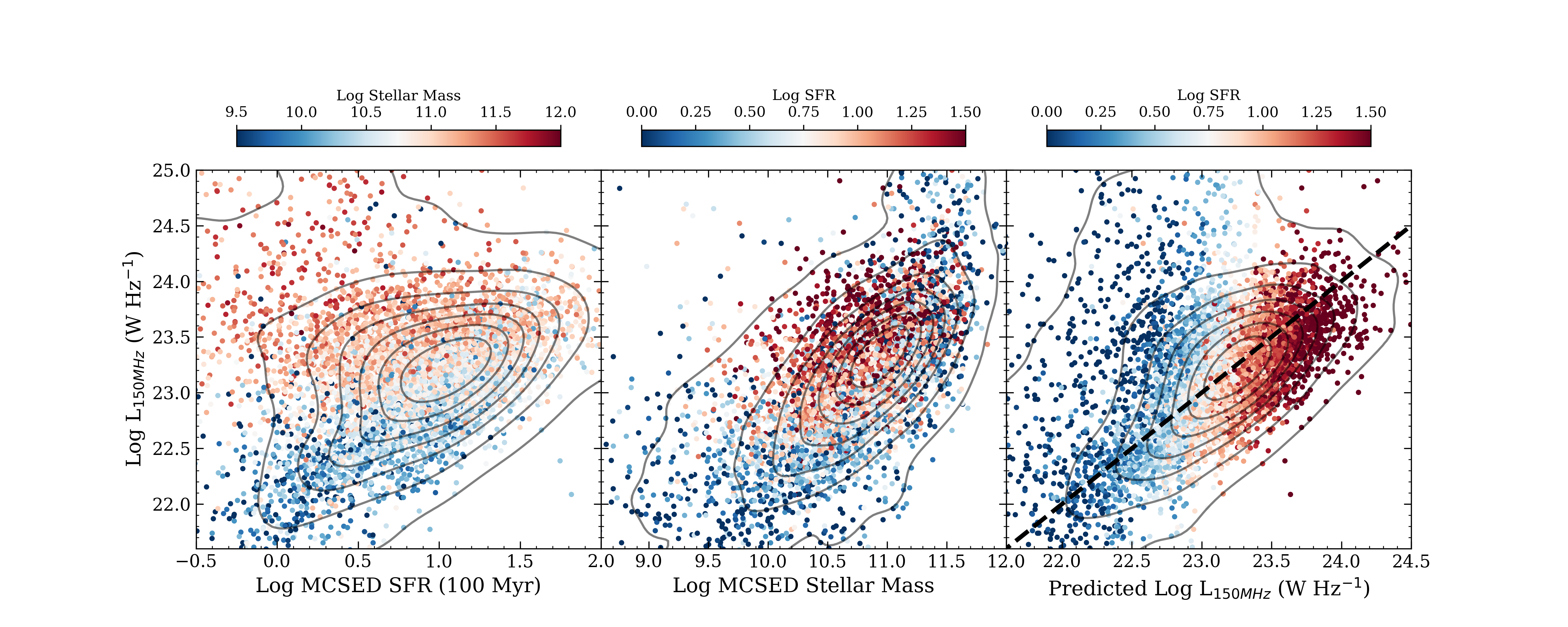
For our sample of galaxies, we used the MCSED results to examine the correlation between 150 MHz luminosity and SFR, as well as the secondary stellar mass dependence. Figure 8 shows the results for each of these relationships. All of the galaxies studied have SFR and stellar mass estimates that were derived from energy balance spectral energy distribution fitting using redshifts and aperture-matched forced photometry from the LOFAR Two-metre Sky Survey (LoTSS) Deep Fields data release. The first panel in Figure 8 shows the correlation between SFR and 150 MHz luminosity. There is tight correlation between the two quantities, though there is some scatter caused by the secondary mass dependence acknowledged by Smith et al. (2021). This mass dependence can be seen via the color bar. The second panel demonstrates the correlation between stellar mass and 150 MHz luminosity. There is a strong correlation here, which is to be expected as we anticipate a secondary mass dependence. Additionally, we referenced the Smith et al. (2021) calculation for 150 MHz luminosity to determine the predicted luminosity expected for our MCSED results which is shown in the third panel. The black dashed line represents a one-to-one correlation. All of our data follows this trend and is tightly correlated. This comparison acts as a check on our derived values for 150 MHz luminosity, stellar mass, and SFR. The majority of our derived values match closely to those predicted by the Smith relation. Overall, we were able to measure SFR, 150 MHz luminosity, and stellar mass for 6,499 galaxies.

4.3 Line Ratio Diagnostics

We used PPXF to measure the line fluxes for our individual galaxies, particularly focusing on the [O III], [O II], and [Ne III] emission lines. We measure these lines in particular due to their use in radio astronomy. [O III] is used to trace ionized outflows from radio sources because of its sensitivity to the impact of radiation and jets (e.g., Kukreti et al., 2023). Additionally, these three lines can be useful in line ratios as indicators of ionization parameter. The most commonly used diagnostic of the ionization parameter is [O III]/[O II] (O3O2) (e.g., Alloin et al., 1978; Baldwin et al., 1981); however, the wavelength range between [O III] and [O II] makes this line ratio diagnostic radio sensitive to extinction effects. As an alternative, [Ne III]/[O II] (Ne3O2) can act as a similar diagnostic of ionization parameter that is radio insensitive to reddening effects (e.g., Levesque & Richardson, 2014). The similar short wavelengths of [Ne III] and [O II] also make the diagnostic usable at larger redshifts (z $\sim$ 1.6) than O3O2 (Nagao et al., 2006). The benefits of Ne3O2 as a diagnostic of ionization parameter as compared to those of O3O2 led us to solely examine the Ne3O2 line ratio in our sample. Because many of the measured lines are weak, we also computed the biweight stack of the HETDEX spectra binned by stellar mass, with each spectrum normalized by its median continuum value in the rest-frame wavelength range of $3750\,{\rm\AA}<\lambda<3850$ Å for Ne3O2. We also limited our sample to galaxies with $z<0.4$ to ensure we detect the [Ne III] and [O II] lines.

The line ratio diagnostics used are indicators of ionization and relationship to AGN activity; however, they are not definitive criteria to determine contribution from AGN activity. To further understand the properties of our data set, we used the relation between SFR and 150 MHz luminosity derived in Best et al. (2023). This relation can be used to set an N- $\sigma$ cutoff above the Best et al. (2023) ridgeline which can help determine which galaxies are star-forming and which are dominated by AGN activity. Galaxies that fall within the N- $\sigma$ cutoff are star-forming, while those above the cutoff have AGN activity.

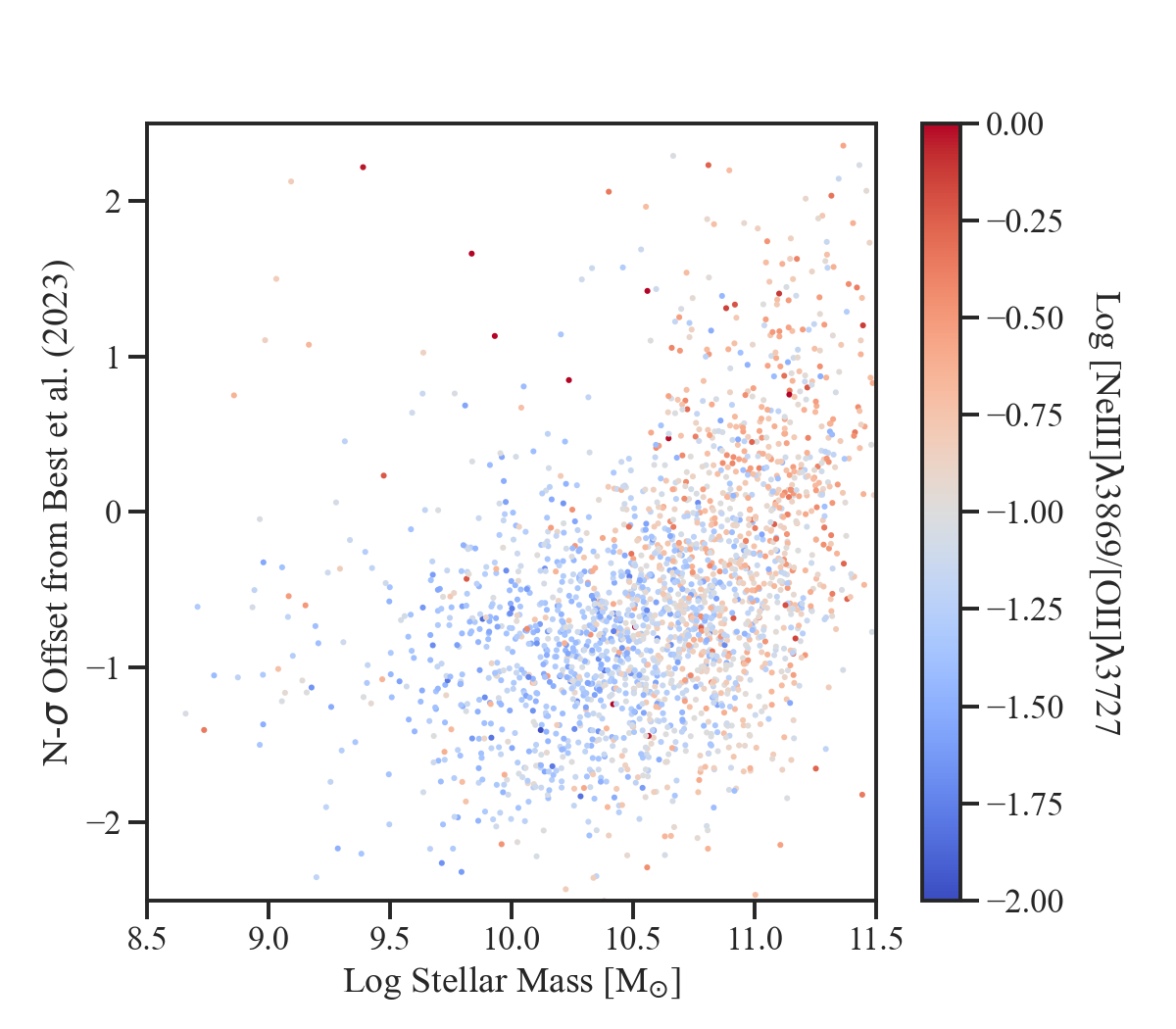
We further explored this relation by examining the relationship between stellar mass and the N- $\sigma$ offset from the Best et al. (2023) relation (Figure 9). AGN typically have harder ionization fields, meaning that the their log₁₀(Ne3O2) line ratios should be greater than 1. By coloring the scatter in Figure 9 by the Ne3O2 ratio, we see that none of the galaxies with $z<0.4$ have log₁₀(Ne3O2) $>1$ ; however, as galaxies reach $\log_{10}(M/M_{\odot})>10.5$ , Ne302 increases with the offset from the Best et al. (2023) relationship. This suggests that there could be a greater contribution from AGN.

4.4 The SFR-150 MHz Luminosity Relation

We determined the SFR-L_150MHz relation as follows. First, we applied a mass cut at log ${}_{10}(M/M_{\odot})<11.0$ . This mass cut arises from the analysis of Figure 9, which shows increasing AGN contribution above log₁₀ $(M/M_{\odot})\approx 10.5$ . To ensure that our fit was based mostly on star-forming galaxies, we removed the population with potential AGN contribution from our sample used for fitting. For the remaining sources, we calculated the errors on SFR, stellar mass, and L_150MHz and found an average log₁₀ error of $\pm 0.216$ [ $M_{\odot}yr^{-1}$ ] for SFR, $\pm 0.132$ [ $M_{\odot}$ ] for stellar mass, and $\pm 0.070$ [W Hz^-1] for L_150MHz.

To determine best-fit parameters, we adopted the form of the mass-dependent SFR-L_150MHz relationship from Gürkan et al. (2018):

L_{\rm{150MHz}}=L_{C}\psi^{\beta}(\frac{M_{*}}{10^{10}M_{\odot}})^{\gamma}

(1)

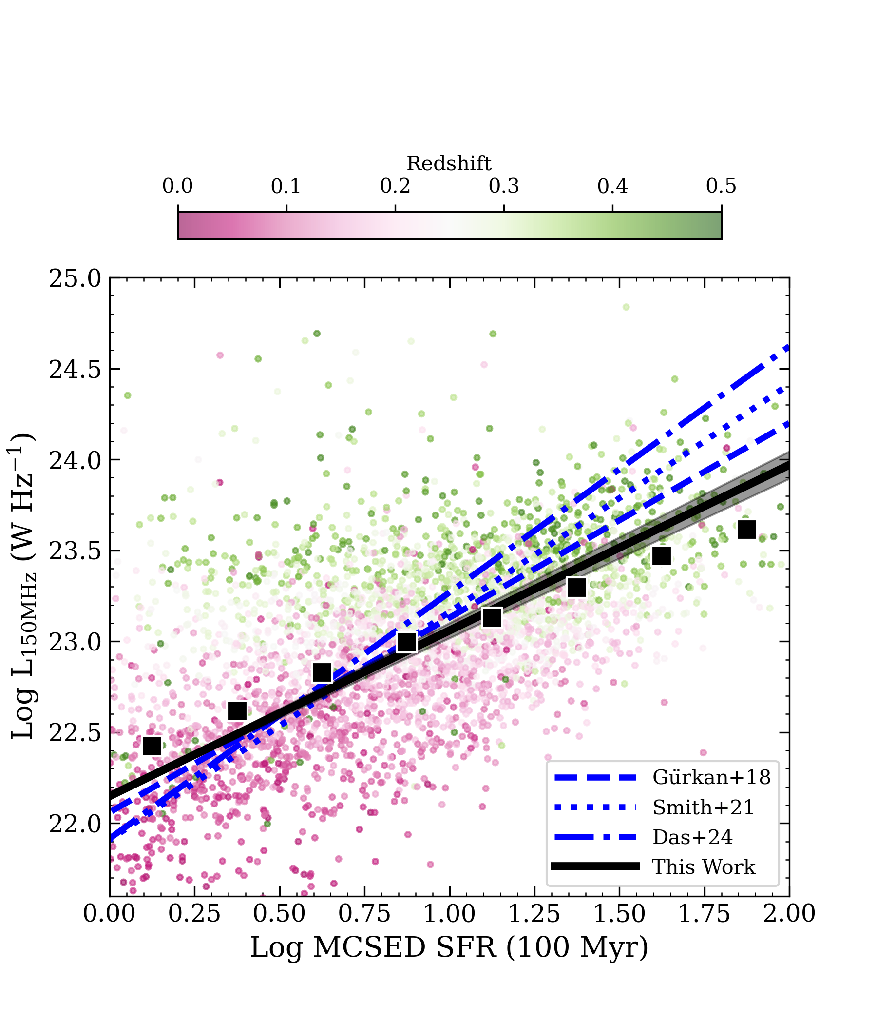
where L_C is the 150 MHz luminosity of a galaxy with $M_{*}=10^{10}M_{\odot}$ and $\psi=1$ $M_{\odot}yr^{-1}$ . We find the best-fit values of log₁₀ $L_{C}=22.341\pm 0.016$ , $\beta=0.526\pm 0.017$ , and $\gamma=0.384\pm 0.017$ , determined using the emcee (Foreman-Mackey et al., 2019) Monte Carlo Markov Chain (MCMC) algorithm with 15 walkers and a chain length of 10,000 samples. Our best fit SFR-L_150MHz relation is, therefore, log ${}_{10}L_{\rm{150MHz}}$ = (22.341 $\pm$ 0.016) + (0.526 $\pm$ 0.017) log₁₀( $\psi$ / $M_{\odot}yr^{-1}$ ) + (0.384 $\pm$ 0.017) log₁₀( $M/10^{10}M_{\odot}$ ).

We compared this mass-dependent line fit to those found by Gürkan et al. (2018), Smith et al. (2021), and Das et al. (2024) in Figure 10. Gürkan et al. (2018) obtained best-fit estimates of log₁₀ $L_{C}=22.13\pm 0.01$ , $\beta=0.77\pm 0.01$ , and $\gamma=0.43\pm 0.01$ . Smith et al. (2021) found best-fit estimates of log₁₀ $L_{C}=22.218\pm 0.016$ , $\beta=0.903\pm 0.012$ , and $\gamma=0.332\pm 0.037$ . Das et al. (2024) obtained best-fit estimates of log₁₀ $L_{C}=22.083\pm 0.004$ , $\beta=0.778\pm 0.004$ , and $\gamma=0.334\pm 0.006$ . Our line has a shallower slope than the three previously derived mass-dependent expressions. This difference could be a result of several factors. Our relation is derived using spectroscopic redshifts with small error, creating an upper radio luminosity limit that is quite sharp (shown by the coloring of data points in Figure 10). This upper limit could be depressing the steepness of our fit because it is creating an upper limit on radio luminosity. There is also a lower limit caused by the flux density limit of our sample. The combination of both the upper and lower limits on luminosity could result in a lack of objects that would tend to populate the lower-left and upper-right of Figure 10. The slope of the fit is most influenced by objects at the extremes of radio luminosity and SFR, so if there is limit-related bias present, the slope will also be biased. Additionally, the applied mass cut could have removed a number of the high luminosity sources, which would also create bias in the slope. The larger sample that will be available with the release of the full HETDEX survey – approximately 40,000 sources – will allow a more thorough analysis of the possible systematic effects in fitting the SFR relation, and this analysis can be investigated further in a future paper.

5 Summary

Combining data from an optical spectroscopic survey, the fourth data release of the Hobby-Eberly Telescope Dark Energy Experiment (HETDEX) catalog and a radio survey, the first data release of the Low Frequency Array Two-metre Sky Survey (LoTSS), we were able to determine intrinsic properties for radio sources present in both fields of view. Using positions in LoTSS we extracted 18,267 spectra from the HETDEX database. We used a robust and automatic classification code called Diagnose, developed by our group for the HET VIRUS Parallel Survey, to determine redshifts and object classifications from the optical spectra. We also use the HETDEX ElixerWidget to source redshifts and object classifications. To determine redshifts and classifications for the remaining unknown spectra, we matched these sources (2″ radius) to object positions in the HETDEX data release 4 catalog. Using these methods, we created the HETDEX-LOFAR Spectroscopic Redshift Catalog with 9,710 total redshift values. We group all sources labeled ‘STAR’ by Diagnose or HDR4 together as ‘STAR’. We group all objects labeled ‘QSO’ or ‘AGN’ in Diagnose or HDR4, respectively, as ‘AGN’; this is done for all redshifts $0.0<z<3.5$ . Classifications of ‘LZG’ and ‘OII’ from HDR4 and ‘GALAXY’ from Diagnose are all grouped under the label ‘LOWZGAL’ for galaxies $0.0<z<0.5$ . Classifications of ‘LAE’ from HDR4 are grouped as ‘HIGHZGAL’ for systems with $1.9<z<3.5$ . Finally, if the redshift comes from the archive, we label the group ‘ARCHIVE’ with $0.0<z<3.5$ . So our final five labels are ‘STAR’, ‘AGN’, ‘LOWZGAL’, ‘HIGHZGAL’, and ‘ARCHIVE’.

The compiled catalog includes 197 ‘STAR’, 804 ‘AGN’, 6,394 ‘LOWZGAL’, 1,075 ‘HIGHZGAL’, and 757 ‘ARCHIVE’ sources.

The focus of this project is assigning redshifts for sources, which, for extragalactic objects, allows one to determine distances and hence many intrinsic properties, most importantly the luminosity. Using line ratio diagnostics such as [Ne III]/[O II], we probed the ionization parameter of the gas. These properties enable AGN excitation to be detected within the star-forming galaxies.

The HETDEX-LOFAR Spectroscopic Redshift Catalog contains the highest substantial fraction of LOFAR galaxies with spectroscopic redshift information and coverage. The catalog also offers an improvement over the archival spectroscopic redshift estimates provided in the LoTSS value-added catalog. It also enables the investigation of SFR tracers with high quality data, though the results may not be definitive. We derive the SFR, stellar masses, 150 MHz luminosity, and emission lines for $\sim 75\%$ of our sources with $z<0.4$ , as well as fit a new SFR-L_150MHz relationship. Understanding the relationship between radio luminosities and SFR is increasingly important in the upcoming era of SKA, and this work acts as the first step to help inform future work in the radio community such as investigating the connection between ionized outflows traced by [O III] and radio emission, refining radio luminosity functions, and comparison of spectra with resolved sub-galactic radio emission. All of the values derived through this work can act as a reference point for adjusting star formation surveys.

The HETDEX-LOFAR Spectroscopic Redshift Catalog provides key physical properties of 9,710 including RA, Dec, spectroscopic redshift, classification, stellar mass, SFR, and 150 MHz luminosity. These properties will serve to enable science investigations in the radio astronomy community.

5.1 Data Release

The fourth internal data release of HETDEX covers $\sim 90\%$ of the total survey, making this the first paper in a series about combining HETDEX and LoTSS. By the time HETDEX finishes, we anticipate a final HETDEX-LOFAR sample of $\sim$ 40,000 galaxies. This paper includes the release of derived spectroscopic redshifts, classifications, stellar masses, SFR, 150 MHz luminosity, and line fluxes for each source, as well as the spectra. A copy of the HETDEX-LOFAR Spectroscopic Redshift Catalog is available on Zenodo doi:10.5281/zenodo.13619775. This Zenodo deposit includes a FITS file with the spectra for all 28,705 sources, as well as the derived redshifts, classifications, and MCSED quantities for each source (columns described in Table 2). The deposit also includes the required statements and papers to reference to acknowledge use of data from the HETDEX survey.

Acknowledgments

HETDEX is led by the University of Texas at Austin McDonald Observatory and Department of Astronomy with participation from the Ludwig-Maximilians-Universität München, Max-Planck-Institut für Extraterrestrische Physik (MPE), Leibniz-Institut für Astrophysik Potsdam (AIP), Texas A&M University, Pennsylvania State University, Institut für Astrophysik Göttingen, The University of Oxford, Max-Planck-Institut für Astrophysik (MPA), The University of Tokyo and Missouri University of Science and Technology.

Observations for HETDEX were obtained with the Hobby-Eberly Telescope (HET), which is a joint project of the University of Texas at Austin, the Pennsylvania State University, Ludwig-Maximillians-Universität München, and Georg-August-Universität, Göttingen. The HET is named in honor of its principal benefactors, William P. Hobby and Robert E. Eberly. We thank the staff at McDonald Observatory for making this project possible. The Visible Integral-field Replicable Unit Spectrograph (VIRUS) was used for HETDEX observations. VIRUS is a joint project of the University of Texas at Austin, Leibniz-Institut für Astrophysik Potsdam (AIP), Texas A&M University, Max-Planck-Institut für Extraterrestrische Physik (MPE), Ludwig-Maximilians-Universität München, Pennsylvania State University, Institut für Astrophysik Göttingen, University of Oxford, and the Max-Planck-Institut für Astrophysik (MPA).

Funding for HETDEX has been provided by the partner institutions, the National Science Foundation, the State of Texas, the US Air Force, and by generous support from private individuals and foundations.

The authors acknowledge the Texas Advanced Computing Center (TACC) at The University of Texas at Austin for providing computing resources that have contributed to the research results reported within this paper. URL:http://www.tacc.utexas.edu.

The Institute for Gravitation and the Cosmos is supported by the Eberly College of Science and the Office of the Senior Vice President for Research at the Pennsylvania State University.

The Pan-STARRS1 Surveys (PS1) and the PS1 public science archive have been made possible through contributions by the Institute for Astronomy, the University of Hawaii, the Pan-STARRS Project Office, the Max-Planck Society and its participating institutes, the Max Planck Institute for Astronomy, Heidelberg and the Max Planck Institute for Extraterrestrial Physics, Garching, The Johns Hopkins University, Durham University, the University of Edinburgh, the Queen’s University Belfast, the Harvard-Smithsonian Center for Astrophysics, the Las Cumbres Observatory Global Telescope Network Incorporated, the National Central University of Taiwan, the Space Telescope Science Institute, the National Aeronautics and Space Administration under Grant No. NNX08AR22G issued through the Planetary Science Division of the NASA Science Mission Directorate, the National Science Foundation Grant No. AST-1238877, the University of Maryland, Eotvos Lorand University (ELTE), the Los Alamos National Laboratory, and the Gordon and Betty Moore Foundation.

We also thank the Erickson Discovery Grant for providing support to complete this project during Summer 2022. Funding from this grant paved the path to complete the majority of analysis required for this project.

References

Abolfathi et al. (2018) Abolfathi, B., Aguado, D. S., Aguilar, G., et al. 2018, ApJS, 235, 42, doi: 10.3847/1538-4365/aa9e8a
Alloin et al. (1978) Alloin, D., Bergeron, J., & Pelat, D. 1978, A&A, 70, 141
Almeida et al. (2023) Almeida, A., Anderson, S. F., Argudo-Fernández, M., et al. 2023, ApJS, 267, 44, doi: 10.3847/1538-4365/acda98
Baldwin et al. (1981) Baldwin, J. A., Phillips, M. M., & Terlevich, R. 1981, PASP, 93, 5, doi: 10.1086/130766
Bertelli et al. (1994) Bertelli, G., Bressan, A., Chiosi, C., Fagotto, F., & Nasi, E. 1994, A&AS, 106, 275
Best et al. (2014) Best, P. N., Ker, L. M., Simpson, C., Rigby, E. E., & Sabater, J. 2014, MNRAS, 445, 955, doi: 10.1093/mnras/stu1776
Best et al. (2023) Best, P. N., Kondapally, R., Williams, W. L., et al. 2023, MNRAS, 523, 1729, doi: 10.1093/mnras/stad1308
Bolton et al. (2012) Bolton, A. S., Schlegel, D. J., Aubourg, É., et al. 2012, AJ, 144, 144, doi: 10.1088/0004-6256/144/5/144
Bonzini et al. (2013) Bonzini, M., Padovani, P., Mainieri, V., et al. 2013, MNRAS, 436, 3759, doi: 10.1093/mnras/stt1879
Botteon et al. (2020) Botteon, A., van Weeren, R. J., Brunetti, G., et al. 2020, MNRAS, 499, L11, doi: 10.1093/mnrasl/slaa142
Bowman et al. (2020) Bowman, W. P., Zeimann, G. R., Nagaraj, G., et al. 2020, ApJ, 899, 7, doi: 10.3847/1538-4357/ab9f3c
Byler et al. (2017) Byler, N., Dalcanton, J. J., Conroy, C., & Johnson, B. D. 2017, ApJ, 840, 44, doi: 10.3847/1538-4357/aa6c66
Calzetti et al. (2000) Calzetti, D., Armus, L., Bohlin, R. C., et al. 2000, ApJ, 533, 682, doi: 10.1086/308692
Cappellari (2023) Cappellari, M. 2023, MNRAS, 526, 3273, doi: 10.1093/mnras/stad2597
Chabrier (2003) Chabrier, G. 2003, PASP, 115, 763, doi: 10.1086/376392
Chambers et al. (2016) Chambers, K. C., Magnier, E. A., Metcalfe, N., et al. 2016, arXiv e-prints, arXiv:1612.05560. https://arxiv.org/abs/1612.05560
Condon et al. (2002) Condon, J. J., Cotton, W. D., & Broderick, J. J. 2002, AJ, 124, 675, doi: 10.1086/341650
Conroy & Gunn (2010) Conroy, C., & Gunn, J. E. 2010, FSPS: Flexible Stellar Population Synthesis, Astrophysics Source Code Library, record ascl:1010.043
Conroy et al. (2009) Conroy, C., Gunn, J. E., & White, M. 2009, ApJ, 699, 486, doi: 10.1088/0004-637X/699/1/486
Cordun et al. (2023) Cordun, C. M., Timmerman, R., Miley, G. K., et al. 2023, A&A, 676, A29, doi: 10.1051/0004-6361/202346320
Dalton et al. (2012) Dalton, G., Trager, S. C., Abrams, D. C., et al. 2012, in Society of Photo-Optical Instrumentation Engineers (SPIE) Conference Series, Vol. 8446, Ground-based and Airborne Instrumentation for Astronomy IV, ed. I. S. McLean, S. K. Ramsay, & H. Takami, 84460P, doi: 10.1117/12.925950
Dalton et al. (2014) Dalton, G., Trager, S., Abrams, D. C., et al. 2014, in Society of Photo-Optical Instrumentation Engineers (SPIE) Conference Series, Vol. 9147, Ground-based and Airborne Instrumentation for Astronomy V, ed. S. K. Ramsay, I. S. McLean, & H. Takami, 91470L, doi: 10.1117/12.2055132
Das et al. (2024) Das, S., Smith, D. J. B., Haskell, P., et al. 2024, MNRAS, 531, 977, doi: 10.1093/mnras/stae1204
Davies et al. (2017) Davies, G. R., Lund, M. N., Miglio, A., et al. 2017, A&A, 598, L4, doi: 10.1051/0004-6361/201630066
Davis et al. (2023) Davis, D., Gebhardt, K., Cooper, E. M., et al. 2023, ApJ, 946, 86, doi: 10.3847/1538-4357/acb0ca
De Zotti et al. (2019) De Zotti, G., Bonato, M., & Cai, Z.-Y. 2019, in 3rd Cosmology School, Introduction to Cosmology, ed. K. Bajan, M. Biernacka, & A. Pollo, Vol. 9, 125–150, doi: 10.48550/arXiv.1802.06561
Debski & Zeimann (2024) Debski, M., & Zeimann, G. 2024, Diagnose. https://doi.org/10.5281/zenodo.13755510
Draine & Li (2007) Draine, B. T., & Li, A. 2007, ApJ, 657, 810, doi: 10.1086/511055
Duncan et al. (2019) Duncan, K. J., Sabater, J., Röttgering, H. J. A., et al. 2019, A&A, 622, A3, doi: 10.1051/0004-6361/201833562
Feretti et al. (2012) Feretti, L., Giovannini, G., Govoni, F., & Murgia, M. 2012, A&A Rev., 20, 54, doi: 10.1007/s00159-012-0054-z
Ferland et al. (1998) Ferland, G. J., Korista, K. T., Verner, D. A., et al. 1998, PASP, 110, 761, doi: 10.1086/316190
Ferland et al. (2013) Ferland, G. J., Porter, R. L., van Hoof, P. A. M., et al. 2013, Rev. Mexicana Astron. Astrofis., 49, 137, doi: 10.48550/arXiv.1302.4485
Foreman-Mackey et al. (2013) Foreman-Mackey, D., Hogg, D. W., Lang, D., & Goodman, J. 2013, PASP, 125, 306, doi: 10.1086/670067
Foreman-Mackey et al. (2019) Foreman-Mackey, D., Farr, W., Sinha, M., et al. 2019, The Journal of Open Source Software, 4, 1864, doi: 10.21105/joss.01864
Gebhardt et al. (2021) Gebhardt, K., Mentuch Cooper, E., Ciardullo, R., et al. 2021, ApJ, 923, 217, doi: 10.3847/1538-4357/ac2e03
Girardi et al. (2000) Girardi, L., Bressan, A., Bertelli, G., & Chiosi, C. 2000, VizieR Online Data Catalog: Low-mass stars evolutionary tracks & isochrones (Girardi+, 2000), VizieR On-line Data Catalog: J/A+AS/141/371. Originally published in: 2000A&AS..141..371G
Gloudemans et al. (2021) Gloudemans, A. J., Duncan, K. J., Röttgering, H. J. A., et al. 2021, A&A, 656, A137, doi: 10.1051/0004-6361/202141722
Grainge et al. (2017) Grainge, K., Alachkar, B., Amy, S., et al. 2017, Astronomy Reports, 61, 288, doi: 10.1134/S1063772917040059
Gürkan et al. (2018) Gürkan, G., Hardcastle, M. J., Smith, D. J. B., et al. 2018, MNRAS, 475, 3010, doi: 10.1093/mnras/sty016
Heesen et al. (2014) Heesen, V., Brinks, E., Leroy, A. K., et al. 2014, AJ, 147, 103, doi: 10.1088/0004-6256/147/5/103
Hill et al. (2021) Hill, G. J., Lee, H., MacQueen, P. J., et al. 2021, AJ, 162, 298, doi: 10.3847/1538-3881/ac2c02
Horne (1986) Horne, K. 1986, PASP, 98, 609, doi: 10.1086/131801
Kukreti et al. (2023) Kukreti, P., Morganti, R., Tadhunter, C., & Santoro, F. 2023, A&A, 674, A198, doi: 10.1051/0004-6361/202245691
Levesque & Richardson (2014) Levesque, E. M., & Richardson, M. L. A. 2014, ApJ, 780, 100, doi: 10.1088/0004-637X/780/1/100
Marigo et al. (2008) Marigo, P., Girardi, L., Bressan, A., et al. 2008, A&A, 482, 883, doi: 10.1051/0004-6361:20078467
Mentuch Cooper et al. (2023) Mentuch Cooper, E., Gebhardt, K., Davis, D., et al. 2023, ApJ, 943, 177, doi: 10.3847/1538-4357/aca962
Mingo et al. (2019) Mingo, B., Croston, J. H., Hardcastle, M. J., et al. 2019, MNRAS, 488, 2701, doi: 10.1093/mnras/stz1901
Mingo et al. (2022) Mingo, B., Croston, J. H., Best, P. N., et al. 2022, MNRAS, 511, 3250, doi: 10.1093/mnras/stac140
Moffat (1969) Moffat, A. F. J. 1969, A&A, 3, 455
Momcheva et al. (2016) Momcheva, I. G., Brammer, G. B., van Dokkum, P. G., et al. 2016, ApJS, 225, 27, doi: 10.3847/0067-0049/225/2/27
Nagao et al. (2006) Nagao, T., Maiolino, R., & Marconi, A. 2006, A&A, 459, 85, doi: 10.1051/0004-6361:20065216
Padovani et al. (2015) Padovani, P., Bonzini, M., Kellermann, K. I., et al. 2015, MNRAS, 452, 1263, doi: 10.1093/mnras/stv1375
Padovani et al. (2011) Padovani, P., Miller, N., Kellermann, K. I., et al. 2011, ApJ, 740, 20, doi: 10.1088/0004-637X/740/1/20
Pannella et al. (2009) Pannella, M., Carilli, C. L., Daddi, E., et al. 2009, ApJ, 698, L116, doi: 10.1088/0004-637X/698/2/L116
Planck Collaboration et al. (2020) Planck Collaboration, Aghanim, N., Akrami, Y., et al. 2020, A&A, 641, A6, doi: 10.1051/0004-6361/201833910
Ramsey et al. (1998) Ramsey, L. W., Adams, M. T., Barnes, T. G., et al. 1998, in Society of Photo-Optical Instrumentation Engineers (SPIE) Conference Series, Vol. 3352, Advanced Technology Optical/IR Telescopes VI, ed. L. M. Stepp, 34–42, doi: 10.1117/12.319287
Sabater et al. (2019) Sabater, J., Best, P. N., & LOFAR Collaboration. 2019, in Highlights on Spanish Astrophysics X, ed. B. Montesinos, A. Asensio Ramos, F. Buitrago, R. Schödel, E. Villaver, S. Pérez-Hoyos, & I. Ordóñez-Etxeberria, 231–231
Shimwell et al. (2017) Shimwell, T. W., Röttgering, H. J. A., Best, P. N., et al. 2017, A&A, 598, A104, doi: 10.1051/0004-6361/201629313
Shimwell et al. (2019) Shimwell, T. W., Tasse, C., Hardcastle, M. J., et al. 2019, A&A, 622, A1, doi: 10.1051/0004-6361/201833559
Slee et al. (2001) Slee, O. B., Roy, A. L., Murgia, M., Andernach, H., & Ehle, M. 2001, AJ, 122, 1172, doi: 10.1086/322105
Smith et al. (2016) Smith, D. J. B., Best, P. N., Duncan, K. J., et al. 2016, in SF2A-2016: Proceedings of the Annual meeting of the French Society of Astronomy and Astrophysics, ed. C. Reylé, J. Richard, L. Cambrésy, M. Deleuil, E. Pécontal, L. Tresse, & I. Vauglin, 271–280. https://arxiv.org/abs/1611.02706
Smith et al. (2021) Smith, D. J. B., Haskell, P., Gürkan, G., et al. 2021, A&A, 648, A6, doi: 10.1051/0004-6361/202039343
Timmerman et al. (2022) Timmerman, R., van Weeren, R. J., Botteon, A., et al. 2022, A&A, 668, A65, doi: 10.1051/0004-6361/202243936
Timmerman et al. (2024) —. 2024, arXiv e-prints, arXiv:2403.03242, doi: 10.48550/arXiv.2403.03242
Venemans et al. (2007) Venemans, B. P., Röttgering, H. J. A., Miley, G. K., et al. 2007, A&A, 461, 823, doi: 10.1051/0004-6361:20053941
Whyley et al. (2024) Whyley, A., Randall, S. W., Clarke, T. E., et al. 2024, arXiv e-prints, arXiv:2402.04876, doi: 10.48550/arXiv.2402.04876
Williams et al. (2019) Williams, W. L., Hardcastle, M. J., Best, P. N., et al. 2019, A&A, 622, A2, doi: 10.1051/0004-6361/201833564
Wright et al. (2010) Wright, E. L., Eisenhardt, P. R. M., Mainzer, A. K., et al. 2010, AJ, 140, 1868, doi: 10.1088/0004-6256/140/6/1868
Wylezalek et al. (2013) Wylezalek, D., Galametz, A., Stern, D., et al. 2013, ApJ, 769, 79, doi: 10.1088/0004-637X/769/1/79
Yue et al. (2023) Yue, M., Eilers, A.-C., Simcoe, R. A., et al. 2023, ApJ, 950, 105, doi: 10.3847/1538-4357/accf20
Yun et al. (2001) Yun, M. S., Reddy, N. A., & Condon, J. J. 2001, ApJ, 554, 803, doi: 10.1086/323145
Zeimann et al. (2024) Zeimann, G. R., Debski, M. H., Schneider, D. P., et al. 2024, ApJ, 966, 14, doi: 10.3847/1538-4357/ad35b8

\twocolumngrid

Appendix A Diagnose and HDR4 Redshift

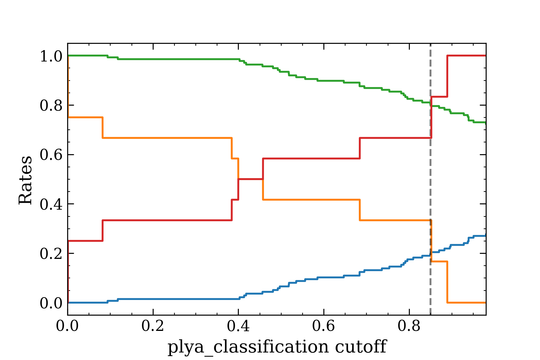
There were 149 sources with $2.0<z_{HDR4}<3.5$ and $0.0<z_{Diagnose}<0.5$ , which demonstrate the common issue of Diagnose identifying an emission line as [O II] while HDR4 identifies the line as Ly $\alpha$ . In order to distinguish which is the best fit redshift for this group, we utilized the HDR4 catalog output ‘plya_classification’ which represents the likelihood of the detected line is Ly $\alpha$ . This criteria ranks each object from 0-1 with 1 being a high probability that the line is Ly $\alpha$ . In order to utilize this probability, we determined a cutoff of ‘plya_classification’ = 0.85 using the HDR4 classification scheme that uses Diagnose redshifts for g-band magnitudes brighter than 22. Figure 12 demonstrates how we determined this cutoff using false positive and false negative rates for different cutoffs.

To determine the rates, we examined each source’s ‘plya_classifcation’ and g-band magnitude at incremental cutoffs between 0 and 1. If the ‘plya_classifcation’ was greater than the cutoff and the g-band magnitude was greater than 22, then we considered this a true positive identification. If the ‘plya_classifcation’ was greater than the cutoff and the g-band magnitude was less than 22, then we considered this a false positive identification. If the ‘plya_classifcation’ was less than the cutoff and the g-band magnitude was less than 22, then we considered this a true negative identification. If the ‘plya_classifcation’ was less than the cutoff and the g-band magnitude was greater than 22, then we considered this a false negative identification. The true positive rate was calculated as true positives divided by the sum of true positives and false negatives. The true negative rate was calculated as true negatives divided by the sum of true negatives and false positives. The false positive rate is 1-true positive rate, and the false negative rate is 1-true negative rate.

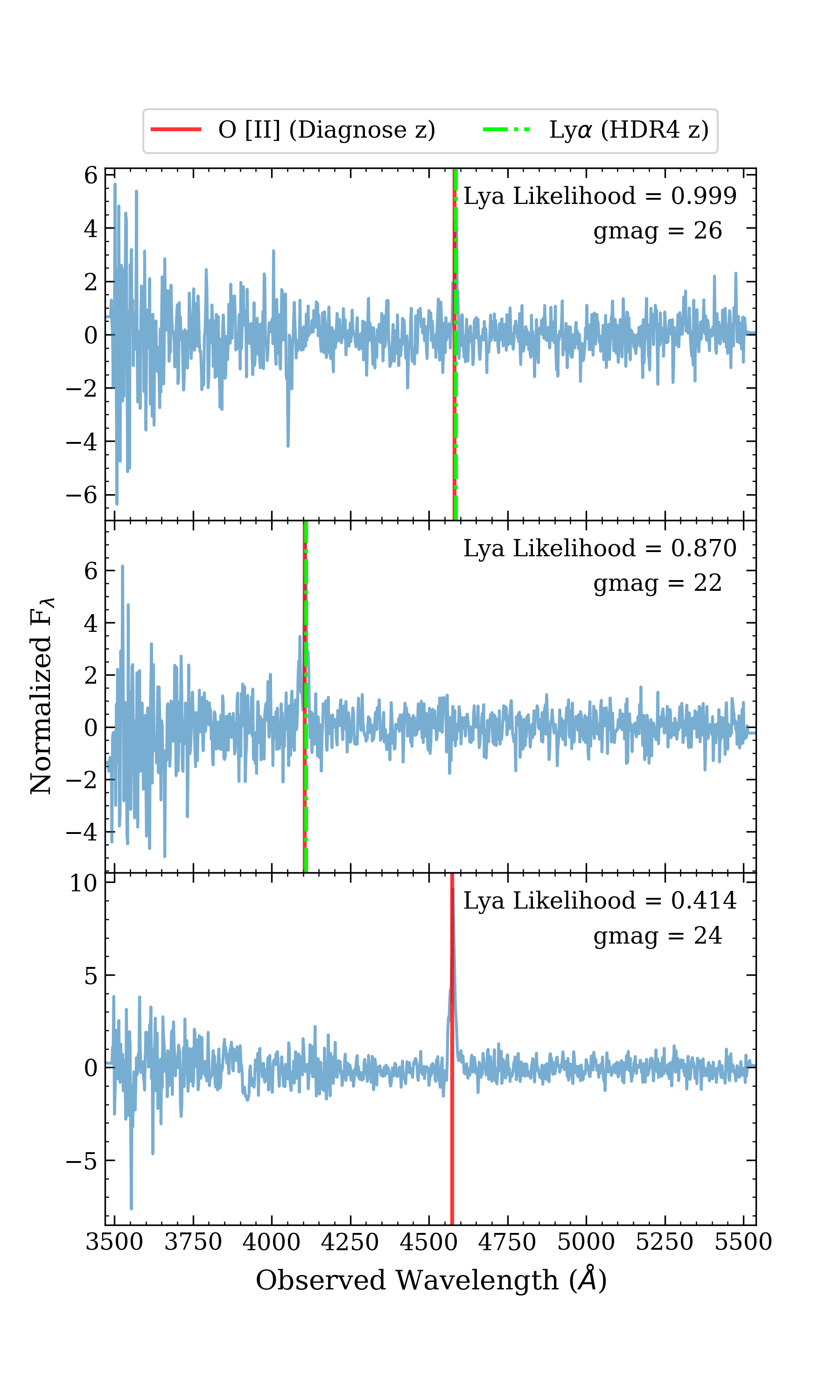
After determining a cutoff for ‘plya_classifcation’, we then proceeded to examine each source in this redshift range by eye. Through this investigation, we determined three patterns to define which redshift to use. Figure 13 shows the three example cases. Using these three patterns, we then determined that for sources that fall within $2.0<z_{HDR4}<3.5$ and $0.0<z_{Diagnose}<0.5$ , if the ‘plya_classifcation’ $<0.85$ , we accept the Diagnose redshift. If ‘plya_classifcation’ $>0.85$ but the g-band magnitude is less than 22, we accept the Diagnose redshift. If ‘plya_classifcation’ $>0.85$ and the g-band magnitude is greater than 22, we accept the HDR4 redshift.

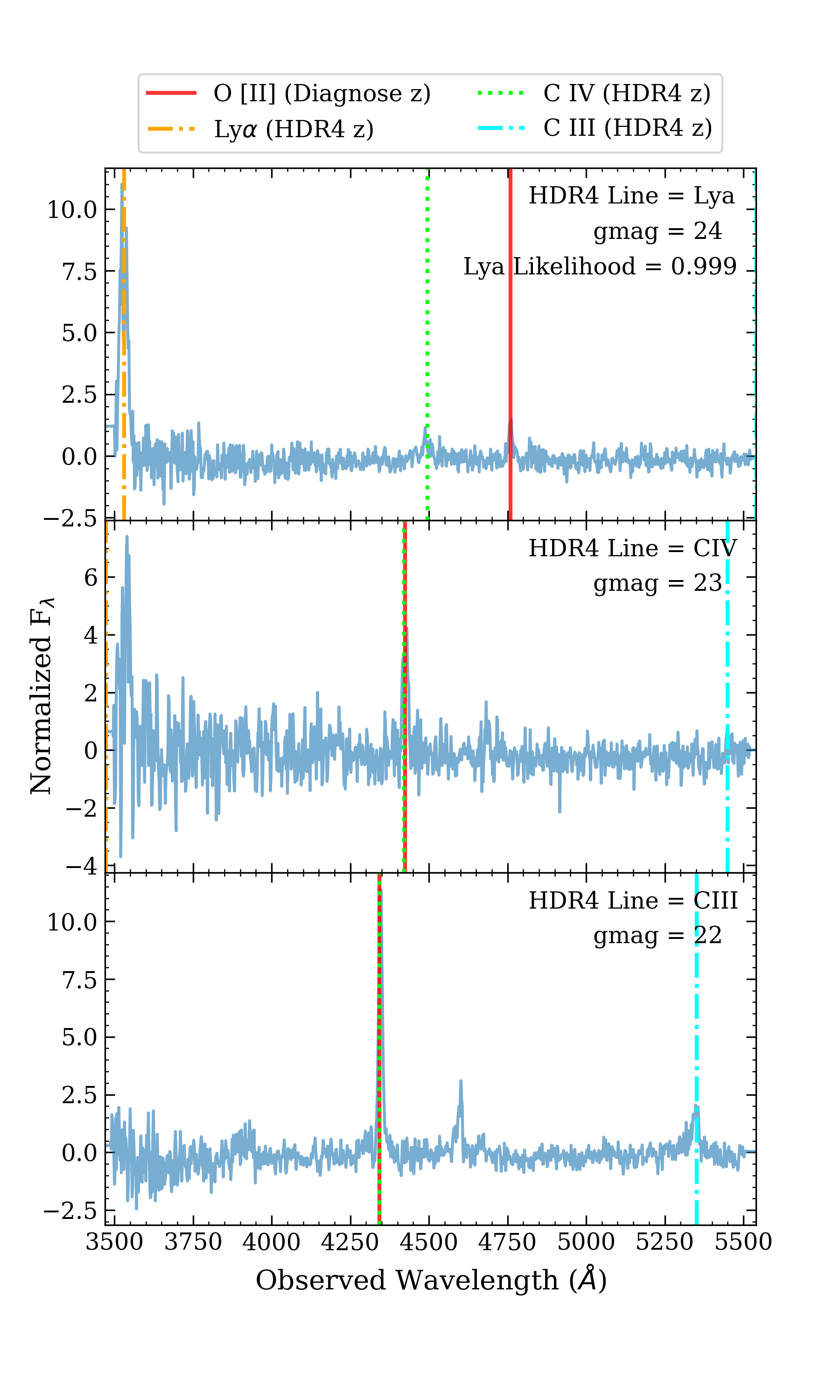
There were 20 sources with $1.5<z_{HDR4}<2.0$ and $0.0<z_{Diagnose}<0.5$ . Some sources in this range also demonstrate the common issue of Diagnose identifying an emission line as [O II] while HDR4 identifies the line as Ly $\alpha$ . In order to distinguish which is the best fit redshift for this group, we utilized the HDR4 catalog output ‘plya_classification’ which represents the likelihood of the detected line is Ly $\alpha$ when HDR4 identifies the emission line as Ly $\alpha$ . After investigating by eye, we determined three patterns to define which redshift to use. Figure 14 shows the three example cases. Using these three patterns, we then determined that for sources that fall within $1.5<z_{HDR4}<2.0$ and $0.0<z_{Diagnose}<0.5$ , if the line identified is Ly $\alpha$ and ‘plya_classifcation’ $<0.85$ , we accept the Diagnose redshift. If the line identified is Ly $\alpha$ and ‘plya_classifcation’ $>0.85$ but the g-band magnitude is less than 22, we accept the Diagnose redshift. If the line identified is Ly $\alpha$ and ‘plya_classifcation’ $>0.85$ and the g-band magnitude is greater than 22, we accept the HDR4 redshift. If the line identified is not Ly $\alpha$ , then we determine solely based on g-band magnitude. If the g-band magnitude is greater than 22, we accept the HDR4 redshift, and if the g-band magnitude is less than 22, we accept the Diagnose redshift.

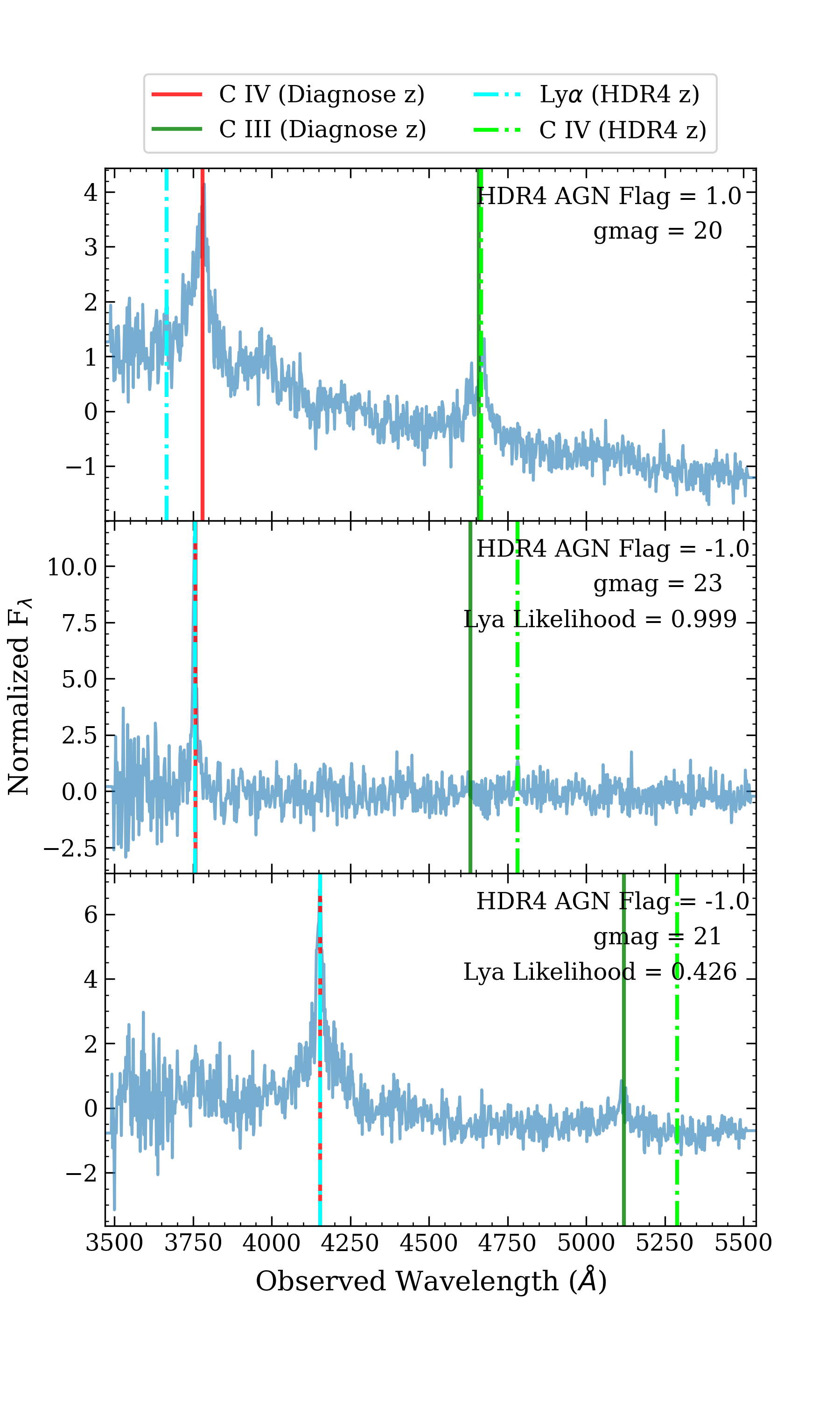
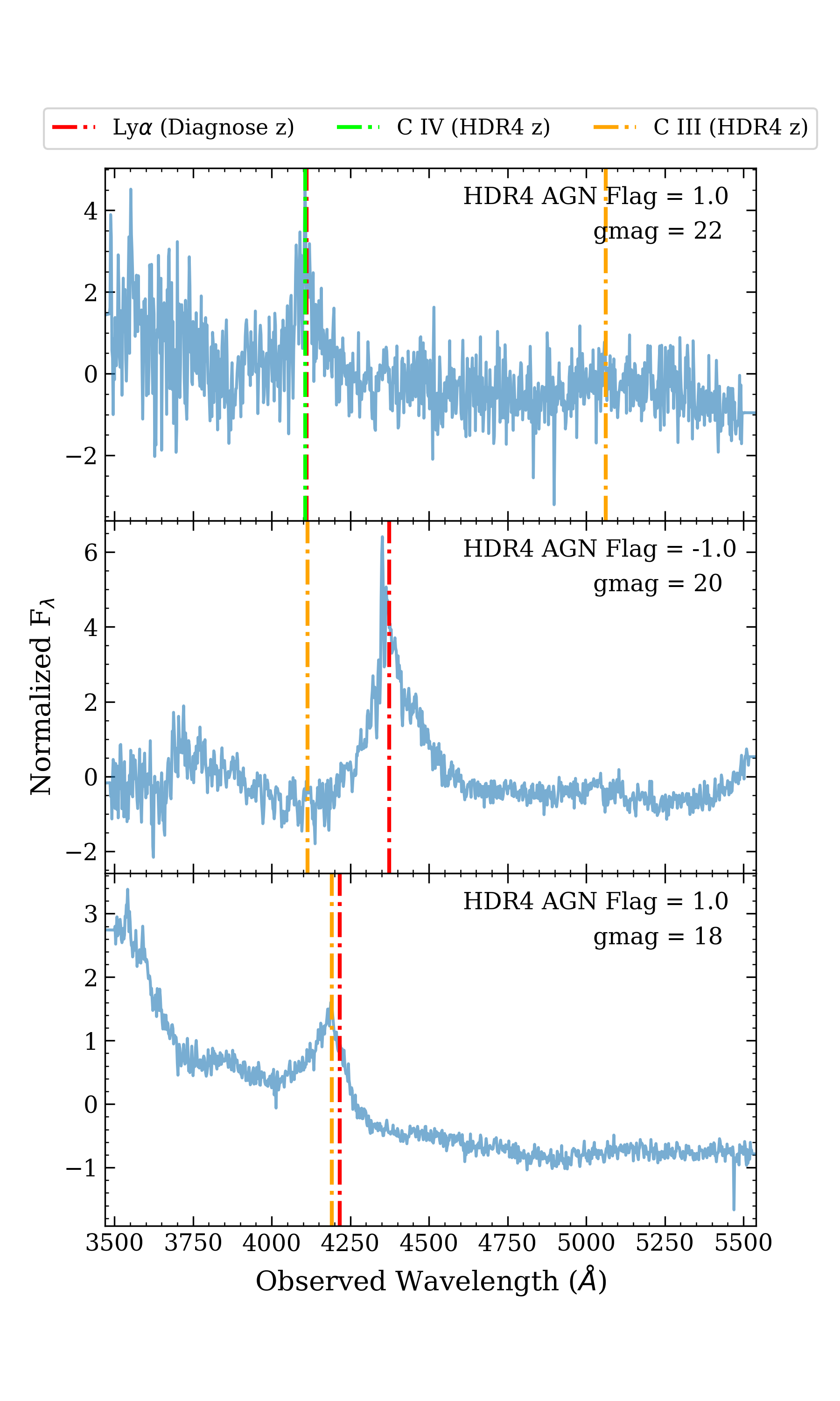
There were 18 sources with $1.5<z_{HDR4}<2.5$ and $1.0<z_{Diagnose}<2.0$ . In order to distinguish which is the best fit redshift for this group, we utilized the HDR4 catalog output ‘agn_flag’ which represents the confidence in the HDR4 AGN classification. A score of 1.0 is a confident AGN, 0.0 is a broadline source but unconfirmed AGN, and -1.0 means it is not an AGN. After investigating by eye, we determined three patterns to define which redshift to use. Figure 15 shows the three example cases. Using these three patterns, we then determined that for sources that fall within $1.5<z_{HDR4}<2.5$ and $1.0<z_{Diagnose}<2.0$ , if ‘agn_flag’ $=1.0$ , we accept the HDR4 redshift. If ‘agn_flag’ $=-1.0$ and ‘plya_classifcation’ $>0.85$ but the g-band magnitude is less than 22, we accept the Diagnose redshift. If ‘agn_flag’ $=-1.0$ and ‘plya_classifcation’ $>0.85$ and the g-band magnitude is greater than 22, we accept the HDR4 redshift.

There were 10 sources with $1.0<z_{HDR4}<2.0$ and $2.0<z_{Diagnose}<3.0$ . In order to distinguish which is the best fit redshift for this group, we utilized the HDR4 catalog output ‘agn_flag’ which represents the confidence in the HDR4 AGN classification. After investigating by eye, we determined two patterns to define which redshift to use. Figure 16 shows the two example cases. Using these two patterns, we then determined that for sources that fall within $1.0<z_{HDR4}<2.0$ and $2.0<z_{Diagnose}<3.0$ , if ‘agn_flag’ $=1.0$ , we accept the HDR4 redshift. If ‘agn_flag’ $=-1.0$ and the g-band magnitude is less than 22, we accept the Diagnose redshift. If ‘agn_flag’ $=-1.0$ and the g-band magnitude is greater than 22, we accept the HDR4 redshift.

We investigated an additional category of 25 sources with $0.0<z_{HDR4}<0.5$ and $1.0<z_{Diagnose}<3.5$ . These sources could not follow a specific set of criteria due to the large range of Diagnose redshifts. Figure 17 shows the spectrum for each object in this group.

HETDEX-LOFAR Spectroscopic Redshift Catalog 111Based on observations obtained with the Hobby-Eberly Telescope, which is a joint project of the University of Texas at Austin, the Pennsylvania State University, Ludwig-Maximilians-Universität München, and Georg-August-Universität Göttingen.