Challenges in constraining dust properties from starlight polarization

Abstract

Context. Dust polarization, which comes from the alignment of aspherical grains to magnetic fields, has been widely employed to study the interstellar medium (ISM) dust properties. The wavelength dependence of the degree of optical polarization, known as the Serkowski relation, was a key observational discovery that advanced grain modeling, and alignment theories. However, it was recently shown that line-of-sight (LOS) variations in the structure of the ISM or the magnetic field morphology contaminate the constraints extracted from fits to the Serkowski relation. These cases can be identified by the wavelength-dependent variability in the polarization angles.

Aims. We aim to investigate to the extent to which we can constrain the intrinsic dust properties, and alignment efficiency from dust polarization data, by accounting for LOS variations of the magnetic field morphology.

Methods. We employed the following archival data: 1) multi-wavelength starlight polarization from the largest agglomerated catalogue to date, 2) 3D dust extinction maps, and 3) stellar parallaxes from Gaia. We fit the Serkowski relation to the polarization data to constrain its free parameters, and explored potential imprints of LOS variations of the magnetic field morphology in them.

Results. We found that these LOS integration effects contaminate the majority of the existing dataset, thus biasing the obtained Serkowski parameters by approximately $10\%$. The constancy of the polarization angles with wavelength does not necessarily guarantee the absence of 3D averaging effects. We examined the efficiency of dust grains in polarizing starlight, as probed by the ratio of the degree of polarization to dust reddening, $E(B-V)$. We found that all measurements respect the limit established by polarized dust emission data. A suppression in polarization efficiencies occurs at $E(B-V)$ $\approx 0.5$ mag. We found evidence that this happens due to projection effects and may be unrelated to the intrinsic alignment of dust grains.

Conclusions. The contribution of multiple LOS clouds to the observed polarization signal contaminates the obtained dust model parameters extracted from the fit of the Serkowski relation. This effect is more prominent in molecular hydrogen sightlines. The only reliable constraints on the intrinsic (aligned) dust grain properties from the existing data can be obtained from diffuse regions with $E(B-V)$ $\lesssim 0.5$ mag. Projection effects are expected to be prominent in polarized dust emission data as well. This result could have important consequences on the interpretations of this dataset and its relation to grain alignment physics. Accurate knowledge of the 3D morphology of the ISM magnetic field is required to probe grain properties from dust polarization.

1 Introduction

Despite accounting for only $\sim 1\%$ of the total (interstellar medium) ISM mass, dust is omnipresent and integral to numerous processes, such as protostar formation (Mouschovias, 1996), molecular cloud dynamics (Hopkins, 2014; Squire & Hopkins, 2018; Hopkins et al., 2022; Hennebelle & Lebreuilly, 2023), cloud thermodynamics, astrochemistry (Goldsmith, 2001; Bialy & Sternberg, 2019), and Galaxy evolution. It is thus imperative to understand the ISM dust grain properties.

Dust polarization is one of the most widely used and accurate methods for investigating the ISM dust grain properties. This effect comes from the interaction between aspherical dust grains and magnetic fields (Andersson et al., 2015). Dust polarization provides important constraints on the ISM grain properties (Guillet et al., 2018; Hensley & Draine, 2021; Hensley & Draine, 2023) and magnetic fields (Davis, 1951; Chandrasekhar & Fermi, 1953; Ostriker et al., 2001; Hildebrand et al., 2009; Houde et al., 2009; Cho & Yoo, 2016; Chen et al., 2022; Panopoulou et al., 2015, 2016; Versteeg et al., 2023; Panopoulou et al., 2019b; Hu & Lazarian, 2023; Pelgrims et al., 2023; Schmaltz et al., 2024; Doi et al., 2024; Skalidis & Pelgrims, 2019; Skalidis & Tassis, 2021; Skalidis et al., 2021). Single-band polarization measurements suffice for magnetic field studies (e.g., Skalidis et al., 2022, 2023), but for the exploration of dust grain properties, multi-band measurements are necessary (Serkowski, 1973; Whittet et al., 1992; Andersson & Potter, 2010).

Variations in the degree of optical dust-induced polarization ($p_{\lambda}$) with wavelength (polarization spectrum) follow an empirical relation, which is usually referred to as the Serkowski relation (Serkowski, 1973; Serkowski et al., 1975). The Serkowski relation provides important constraints on grain properties (Hensley & Draine, 2021; Hensley & Draine, 2023). It reads as follows:

$$p_{\lambda}=p_{max}\leavevmode\nobreak\ \exp\left[-K\leavevmode\nobreak\ \ln^{2}{\left(\frac{\lambda_{max}}{\lambda}\right)}\right],$$ (1)

where $p_{max}$ is the maximum polarization fraction, usually observed at the V-band; $\lambda_{max}$ is the wavelength where $p_{max}$ is observed, and is proportional to the average size of aligned dust grains (Mathis, 1986); $K$ quantifies the spread of $p_{\lambda}$; large $K$ corresponds to narrow profiles, and vice versa. $K$ is considered a proxy for the dust grain size distribution (Serkowski et al., 1975), or for the optical property variations of silicate grains (Papoular, 2018).

Initially, it was found that $K=1.15$ (Serkowski, 1973), but more data suggested a linear relationship between $K$ and $\lambda_{max}$ (Wilking et al., 1980; Whittet et al., 1992; Whittet, 2022),

$$K=(1.66\pm 0.09)\leavevmode\nobreak\ \lambda_{max}+(0.01\pm 0.05).$$ (2)

This is known as the Wilking relation. Eqs. (1), and (2) hold for $\lambda\leavevmode\nobreak\ \epsilon\leavevmode\nobreak\ [0.1,1]$ $\mu$m.

The wavelength dependence of the degree of polarization can be understood as a consequence of the underlying (aligned) grain size distribution. Grain (symmetric and asymmetric) size distributions can be accurately approximated as power laws with negative slopes, indicating that small grains are more abundant than large grains (MRN, Mathis et al., 1977; Weingartner & Draine, 2001). Small grains (nanoparticles) are not easily aligned due to higher collision rates with gas particles (Hoang et al., 2015). Large grains are less susceptible to collisional disalignment but are less abundant. The two effects are balanced for intermediate-sized grains because they are neither too small nor too scarce. Consequently, the maximum degree of polarization is expected for intermediate size grains. In our Galaxy, this optimal size of aligned grains, which is proportional to $\lambda_{max}$, corresponds to $\lambda_{max}$ $\approx$ 0.55 $\mu$m (Whittet, 2022).

The empirical discovery of the polarization fraction’s wavelength dependence by Serkowski et al. (1975) revolutionized multi-wavelength polarization studies; it provided a critical framework for understanding ISM dust and magnetic fields. Soon after this discovery, it became apparent that multi-band polarization is a powerful tool for studying ISM dust, and magnetic fields. The impact of the 3D ISM structure on the Serkowski relation was predicted early on (Clarke & Al-Roubaie, 1984), but observational evidence was limited due to the lack of data. In the last two decades, however, the influx of optical polarization data greatly increased, allowing for systematic explorations of the 3D effects on the $p_{\lambda}$ relation. This is evident by the recent agglomeration of starlight polarization data (Panopoulou et al., 2023), which increased the number of polarization measurements by a factor of five from the previous agglomeration Heiles (2000).

Mandarakas et al. (2024) performed a multi-wavelength starlight polarization study to investigate the impact of the 3D ISM structure, and magnetic field morphology on the Serkowski fits. Through a combination of polarization data, Gaia distances, and 3D dust extinction maps (Edenhofer et al., 2024), Mandarakas et al. (2024) showed that when multiple clouds along the line of sight (LOS) with different magnetic field geometries, or dust properties contribute to the observed polarization signal, $p_{\lambda}$ can either significantly deviate from or accurately follow the Serkowski relation. The latter case is particularly important: it highlights that the standard practice of only fitting the polarization measurements in the $p_{\lambda}$ - $\lambda$ space can be misleading due to the 3D structure of the ISM, even when the fits are accurate. In these cases, variations in the electric vector position angles (EVPA) should be taken into account through a joint fit in the Stokes $Q$, and $U$ space. This result has important consequences for the interpretations of multi-wavelength polarization data, and limits our capacity to probe the intrinsic properties of (aligned) dust.

In light of this discovery, we aimed to assess the accuracy with which we can constrain the intrinsic Serkowski parameters, which is required for grain modeling (Hensley & Draine, 2023); as well as for the alignment efficiency of grains, which is necessary for grain alignment theories (Lazarian & Hoang, 2007; Andersson et al., 2015). We explored the contribution of LOS integration to the obtained Serkowski parameters. In particular, we focused on the correlations between $K$ and $\lambda_{max}$ (Wilking relation, Eq. 2), and the polarization efficiencies, $p_{max}$ / $E(B-V)$. We found that a significant fraction of the existing data is contaminated by LOS variations of the magnetic field morphology, hence it is untrustworthy for constraining the grain properties. Knowledge of the 3D morphology of the ISM magnetic field is required to study the properties of (aligned) dust grains.

The paper is organized as follows: In Sect. 2 we present the employed dataset. In Sect. 3, we fit the Serkowski relation to the data using two methods. In Sect. 4, we explore the correlations between $K$ and $\lambda_{max}$, and we present individual cases of measurements deviating from the Wilking relation because of the contribution of LOS integration. We also show that measurements following the Wilking relation can be affected by these effects. In Sect. 5, we explore the impact of LOS effects on the polarization efficiency obtained from starlight polarization data. We find a suppression in the polarization efficiency of molecular sightlines due to projection effects. In Sects. 6, and 7, we discuss our results in the context of existing literature, and summarize the main outcomes of this work.

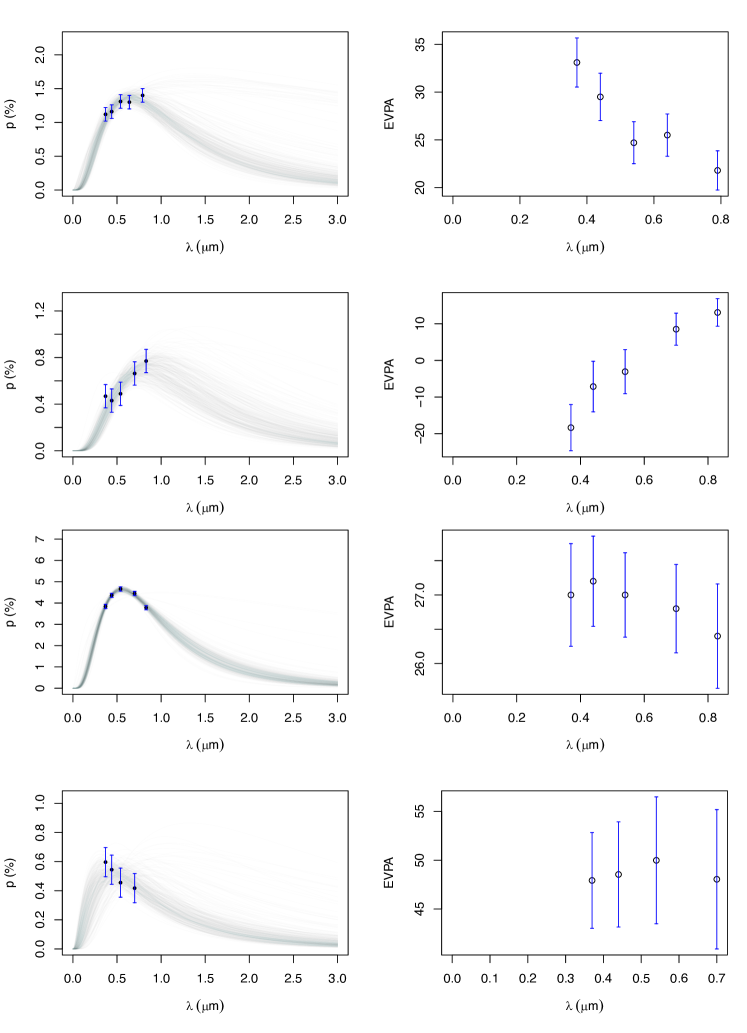
Figure 1: Characteristic examples of good fits ($\chi^{2}\leq 1$). The top two rows shows stars with variable EVPAs ($\Delta\theta$ $>3$), while bottom rows shows stars with constant EVPAs ($\Delta\theta$ $<1$). The third row star (identified as BD+26746), has a higher $K$ / $\lambda_{max}$ ratio than predicted by the Wilking relation. Stars that deviate from the Wilking relation, likely due LOS integration effects, tend to have relatively high degrees of polarization, $p_{max}$ $\gtrsim 2.5\%$ (Sect. 4.1).

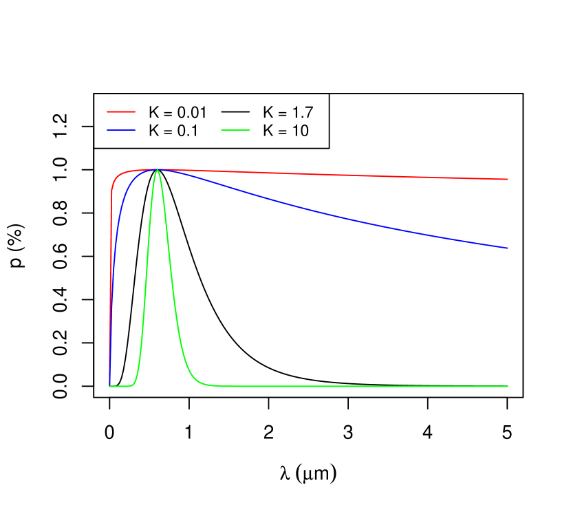
Figure 2: Analytical examples of the Serkowski relation (Eq. 1). The colored curves have different $K$ but fixed $p_{max}$, and $\lambda_{max}$ at $1\%$ and 0.6 $\mu$m respectively. The black curve is typical of the ISM, while other curves, such as red, and green, are extreme cases that are unlike to observe in our Galaxy. Fitting models with only a few data around $\lambda_{max}$, leads to a spectrum of $K$ solutions, which can favor extreme (unphysical) values. For these cases, propagating prior knowledge was crucial for the fits.

2 The multi-wavelength polarization sample

We extracted stars with polarization measurements in more than two bands from the catalogue of Panopoulou et al. (2023). Some stars contain measurements obtained in the same band at different epochs. For these cases, we calculated the average relative Stokes parameters ($\bar{q}$, $\bar{u}$) weighted by their observational uncertainties and then the weighted degree of polarization as $\bar{p}=\sqrt{\bar{q}^{2}+\bar{u}^{2}}$. The observational uncertainty of $\bar{p}$ is (King et al., 2014)

$$\sigma_{p}=\sqrt{\frac{\left(\bar{q}\sigma_{\bar{q}}\right)^{2}+\left(\bar{u}\sigma_{\bar{u}}\right)^{2}}{\left(\bar{q}^{2}+\bar{u}^{2}\right)}}$$ (3)

where $\sigma_{\bar{q}}$, and $\sigma_{\bar{u}}$ correspond to the standard errors of $\bar{q}$ and $\bar{u}$ respectively.

The reported observational uncertainties of some stars were very small, $\sigma_{p}\ll 0.1(\%)$, but as we argue below, they are likely underestimated. The major challenge in achieving such low $\sigma_{p}$ is the instrumental calibration. Even if the instrumental polarization were zero, obtaining observational uncertainties smaller than 0.1$\%$ would be inevitable because of the lack of low-uncertainty polarimetric standard stars.

Until recently, the availability of polarization standard stars was limited, while several stars were proven to be variable at the level of $0.1\%$ (e.g., Blinov et al., 2021, 2023) or had wrong measurements (e.g., Skalidis et al., 2018). A robust polarimetric standard catalogue, which contains 65 stars mostly in the Northern hemisphere, was recently established (Blinov et al., 2023) . This is the most accurate catalogue of optopolarimetric standard stars to date with uncertainties $\sim 0.1\%$, and sets the limit of instrumental calibration. For this reason, we uniformly set polarization uncertainties lower than 0.1 $\%$ to 0.1 $\%$. Be this as it may, our approach is conservative and leads to overestimating the uncertainties in the obtained fits.

2.1 Variability in the position angles

For several stars, EVPAs varied with the wavelength (top two rows in Fig. 1).Variations in EVPA are expected when: 1) different polarization mechanisms contribute to the observed signal (Lopez-Rodriguez, 2016); 2) the observed star has an intrinsic polarization mechanism, such as circumstellar disk, or it is photometrically variable; 3) the magnetic field and dust properties significantly vary along the LOS, hence the polarization signal traces the cumulative effect of the various LOS contributing structures (Patat et al., 2010; Tassis & Pavlidou, 2015; Guillet et al., 2018; Mandarakas et al., 2024).

EVPA variability whether induced by the ISM or other factors, such as those described above, raises questions about the nature of the polarization signal, and how accurately it traces the dust grain properties. To avoid such complications, we identified measurements with variable EVPAs and excluded them from the analysis. We quantified the EVPA variability as:

$$\Delta\theta\equiv\frac{\max(\theta_{\lambda})-\min(\theta_{\lambda})}{\sqrt{\sigma_{\max(\theta_{\lambda})}^{2}+\sigma_{\min(\theta_{\lambda})}^{2}}},$$ (4)

where $\max(\theta_{\lambda})$, and $\min(\theta_{\lambda})$ correspond to the maximum and minimum EVPA across the various wavelength bands, while $\sigma$ denotes the corresponding observational uncertainties .

For $\Delta\theta$ $\leq 1$, any maximum difference in the position angles is consistent within one sigma with the observational uncertainties, and in this case we can confidently consider that EVPAs remain statistically constant across wavelengths (bottom two rows in Fig. 1). On the other hand, when $\Delta\theta$ $>3$, variations in the position angles are statistically significant.

We only focused on sightlines where $\Delta\theta$ $\leq 1$. We considered a flag provided by Panopoulou et al. (2023) to identify intrinsically polarized sources. The total number of measurements of our final sample is 258. Some (19) measurements had no distance information and were not considered in the analysis of Sect 5.

3 Data fitting

We fit the multi-wavelength polarization data with two different ways: 1) in the $p-\lambda$, and 2) $q-u$ space. The latter was proposed by Mandarakas et al. (2024) to account for EVPA variability. We filtered out stars with variable EVPAs (Sect. 2.1), but for comparison we applied both methods.

3.1 $p-\lambda$ fitting

The Serkowski relation (Eq. 1) is characterized by three free parameters. Fitting for these parameters requires measurements in at least three bands. Polarization studies, however, are usually limited to single-band observations because of observing time limitations. Even when multi-band measurements are obtained, the number of observed bands barely exceeds three and in addition, if these bands are obtained with the same instrument, their wavelength separation is not sufficient to accurately trace the $p_{\lambda}$ curves. This is a limitation of the existing dataset, which is the largest to date, that we cannot overcome.

We employed a Bayesian framework to facilitate the fitting process from prior knowledge, and obtain the family of all solutions. This way we can also account for statistical biases that are inherent in low signal-to-noise (S/N) measurements, which have asymmetric confidence intervals in $p$ (Simmons & Stewart, 1985; Plaszczynski et al., 2014).

The Bayes’ theorem reads: the probability, $\mathcal{L}(p_{obs}|p_{\lambda})$, of observing some degree of polarization at a specific wavelength, $p_{obs}$, given some intrinsic value $p_{\lambda}(\@vec{\chi})$, which should follow the Serkowski relation (Eq. 1), is proportional to the joint probability of getting $p_{\lambda}(\@vec{\chi})$ given the observed value, and some prior knowledge on the data, $\mathcal{L}(\@vec{\chi})$; $\@vec{\chi}$ is a vector corresponding to the free parameters of the Serkowski relation, $\@vec{\chi}\equiv(p_{max},K,\lambda_{max})$. The theorem is mathematically expressed as:

$$\mathcal{L}(p_{obs}|p_{\lambda}(\@vec{\chi}))\propto\mathcal{L}(p_{\lambda}(\@vec{\chi})|p_{obs})\leavevmode\nobreak\ \mathcal{L}(\@vec{\chi}).$$ (5)

Our strategy now is to define a physically-motivated likelihood and prior distribution, and then derive the posterior distribution of $\@vec{\chi}$. For computational efficiency, we calculated the logarithms of the probabilities, where Bayes’ theorem becomes:

$$\log{\mathcal{L}(p_{obs}|p_{\lambda}(\@vec{\chi}))}\propto\log{\mathcal{L}(p_{\lambda}(\@vec{\chi})|p_{obs})}+\log{\mathcal{L}(\@vec{\chi})}.$$ (6)

3.1.1 Definition of $p$ likelihood

Gaussian likelihoods are usually employed in Bayesian statistics; this implies symmetric confidence intervals. Polarization fraction, however, is a positive definite quantity, and follows the Rice distribution, which for low S/N is asymmetric, bounded at zero S/N, and has long tails to large values (Rice, 1945). The Rice distribution approximates normal for S/N $\gtrsim 5$ (Appendix A). A large fraction of the employed data has a low S/N ratio; for these cases, we need to consider non-Gaussianities (Simmons & Stewart, 1985; Vaillancourt, 2006; Plaszczynski et al., 2014).

The probability, $\mathcal{L}_{p}(p_{\lambda}(\@vec{\chi})|p_{obs})$, of observing $p_{\lambda}$ is (Vaillancourt, 2006):

$$\mathcal{L}_{p}=\Pi_{j=1}^{N}\frac{1}{N_{L,j}}\frac{p_{obs,j}}{\sigma_{j}^{2}}\exp{\left(\frac{-p_{\lambda}^{2}-(p_{obs,j})^{2}}{2\sigma_{j}^{2}}\right)}\leavevmode\nobreak\ \\ I_{0}\left(\frac{p_{obs,j}p_{\lambda}}{\sigma_{j}^{2}}\right).$$ (7)

$I_{0}$ is the zeroth-order modified Bessel, and $j$ is the index that runs across the various wavelength bands. If, for example, we have $N=3$ polarization measurements (at different bands) then $j=\{1,2,3\}$; $N_{L,j}$ is the normalization factor defined as (Eq. 9, Vaillancourt, 2006)

$$N_{L,j}=p_{obs,j}\sqrt{\frac{\pi}{2}}\exp{\left(-\frac{p_{obs,j}^{2}}{4\sigma_{j}^{2}}\right)}\leavevmode\nobreak\ I_{0}\left(\frac{p_{obs,j}^{2}}{4\sigma_{j}^{2}}\right).$$ (8)

Modified Bessel functions of the first kind, $I_{n}(x)$, grow exponentially, and as a result lead to infinites for large $x$. This can be a major problem in numerical calculations, which become unstable for large $x$. More specifically, in our software – we used the built-in functions of the R programming language to calculate $I_{0}$ – we obtained infinities for $x>700$. This problem was more prominent for the Bessel function shown in Eq. (7) than in $N_{L,j}$ (Eq. 8). To treat these infinities, we used the asymptotic form of $I_{0}$, which is $I_{0}(x)\sim e^{x}/\sqrt{2\pi x}$ for $x\gg 1$. In this case, the likelihood function becomes asymptotic to

$$\mathcal{L}_{p}\sim\Pi_{j=1}^{N}\frac{1}{N_{L}}\sqrt{\frac{p_{obs,j}}{p_{\lambda}}}\frac{1}{\sigma_{j}\sqrt{2\pi}}\exp{\left(-\frac{(p_{obs,j}-p_{\lambda})^{2}}{2\sigma_{j}^{2}}\right)},$$ (9)

which is a Gaussian, with a modified amplitude, and has symmetric confidence intervals (Vaillancourt, 2006). The asymptotic form of the normalization factor is $N_{L,j}\sim\sigma_{j}$. We used the above likelihood when $\sigma_{j}\approx 0.1\%$. The above expression is nearly identical to the Rice distribution for S/N $\geq 5$, and could be used for S/N$\geq 4$. It is more accurate than a normalized Gaussian (Appendix A), and its simplicity makes it useful for future studies.

3.1.2 Distribution of priors

The maximum $p$ value of our extracted sample is $33\%$. For this reason, we assumed a uniform prior distribution for $p_{max}$ ($\%$) in the range [0, 33.0]; $\lambda_{max}$ ranges from 0.3 to 1.0 $\mu$m in our Galaxy (Wilking et al., 1980; Whittet, 2022). To be conservative, we considered a uniform distribution for $\lambda_{max}$ with slightly wider limits: $\lambda\leavevmode\nobreak\ \epsilon\leavevmode\nobreak\ [0.2,1.5]$ $\mu$m.

The employed data usually include a few measurements around the peak of the polarization curve, $\lambda\approx$ $\lambda_{max}$. This is not a problem for constraining $p_{max}$, and $\lambda_{max}$, but $K$ becomes challenging. Without measurements at the near- ultraviolet (UV), and infrared (IR) wavelengths the shape of the polarization spectrum relation can be weakly constrained. Thus, S/N ratios in the obtained $K$ solutions are in general lower than the other two parameters. This problem is better understood by examining some extreme cases.

In the $K\rightarrow 0$ limit, $p\approx p_{max}$ for any $\lambda$, meaning that $p$ is independent of $\lambda$ (red curve in Fig. 2). If only a few measurements were considered around $\lambda_{max}$, then $K\approx 0$ solutions would be favored. The constancy of $p_{\lambda}$ would imply that grain alignment efficiency is independent of the grain size, which is unphysical. In the extreme case where $K\gg 1$, $p_{\lambda}$ approximates a delta function because it rapidly goes to zero everywhere but $\lambda_{max}$, where $p_{\lambda_{max}}\approx p_{max}$ (green curve in Fig. 2); this implies that there is a very narrow range of sizes of dust grains contributing to dust polarization. Neither of these two extreme cases is expected in nature (Whittet, 2022). The lack of near-UV, and near-IR measurements in the fitting process favors the aforementioned unphysical cases. For this reason, considering a more stringent prior distribution for $K$ is necessary for our analysis.

A linear correlation applies between $K$ and $\lambda_{max}$ with a slope close to 1.66 (Wilking et al., 1980), when optical polarization data are used to fit the Serkowski relation. When UV polarimetric data are included in the fits, the slope between the two quantities increases: $K=(2.56\pm 0.38)\leavevmode\nobreak\ \lambda_{max}+(-0.59\pm 0.21)$ (Martin et al., 1999). In both cases the intercept is consistent with zero, but the difference in the slopes is statistically significant; likely induced by the peculiar behavior of dust polarization at UV wavelengths. Differences in the slopes obtained from fits with or without the UV data, become prominent only for $\lambda_{max}$ ¡ 0.5 $\mu$m (Whittet, 2022). This highlights the importance of obtaining UV polarization measurements (Andersson et al., 2022), but observational constraints are limited there. For this reason, we shall restrict ourselves to constraints obtained from optical data (Eq. 2).

We assumed that $K$ linearly correlates with $\lambda_{max}$ as: $K=\alpha\leavevmode\nobreak\ \lambda_{max}$. We assumed that $\alpha$ follows a Gaussian distribution with an average value equal to 1.66, as the optical data suggests (Wilking et al., 1980; Whittet et al., 1992; Whittet, 2022). Intrinsic variations about this slope were determined to be $5\%$, but, to be conservative, we increased the variance to $20\%$. The slope between $K$ and $\lambda_{max}$ is positive definite, $\alpha\geq 0$. Thus, we truncated the Gaussian distribution of $\alpha$ for $\alpha<0$. We only considered measurements with S/N ratio in $p$ equal or larger than three.

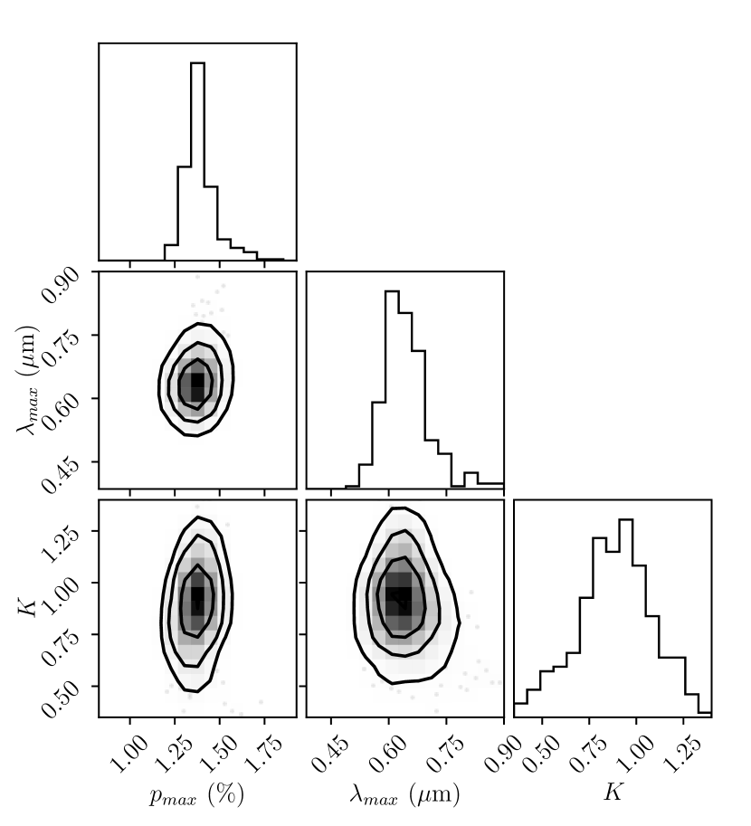
Figure 3: A typical example of the correlations between the posteriors of the free parameters. This case corresponds to a star identified as HD 283643, whose fit is shown in the first row of Fig. 1. The posterior distributions of $p_{max}$, and $\lambda_{max}$ have a well defined peak and are more symmetric than the distribution of $K$, which has an asymmetry toward smaller values. The presence of extended tails in the $K$ distributions is a generic property of nearly all our fits and is induced by the lack of near-UV or -IR polarization measurements (Sect. 3.1.2).

3.1.3 Likelihood maximization and obtained fits

We maximized the log-likelihood (Eq. 6) using the ”BayesianTools” library implemented in R (Hartig et al., 2023). We used the default sampler, DEzs, and initiated 100 walkers, each running for 1000 steps. To ensure the convergence of the walkers, we removed from the posteriors the first 400 steps of the walkers.

We used the chi square to assess the quality of the fits:

$$\chi^{2}=\Sigma_{j}\frac{(p_{\lambda}(\@vec{\chi})-p_{obs,j})^{2}}{\sigma_{j}^{2}}.$$ (10)

Fits with $\chi^{2}\leq 1$ are ”good”, while measurements with $\chi^{2}>1$ are ”bad”, and were excluded from the following analysis. Some examples of good fits are shown in Fig. 1.

3.2 $q-u$ fitting

Constraining the Serkowski parameters through the $q-u$ space is an elaborate way to account for both $p_{\lambda}$, and $\theta_{\lambda}$ variations. Contrary to the degree of polarization, Stokes $q$, and $u$ are characterized by Gaussian likelihoods, which significantly simplifies the calculations. However, only recently was this method applied to multi-wavelength starlight polarization data (Mandarakas et al., 2024). Henceforth, we follow this methodology.

Stokes $q$, and $u$ at a given wavelength are:

$$q_{\lambda}=p_{\lambda}\leavevmode\nobreak\ \cos(2\theta_{\lambda}),$$ (11)

$$u_{\lambda}=p_{\lambda}\leavevmode\nobreak\ \sin(2\theta_{\lambda}).$$ (12)

Substituting the Serkowski formula (Eq. 1) to the above equations yields

$$q_{\lambda}=p_{max}\leavevmode\nobreak\ \exp\left[-K\leavevmode\nobreak\ \ln^{2}\left({\frac{\lambda_{max}}{\lambda}}\right)\right]\leavevmode\nobreak\ \cos(2\theta),$$ (13)

$$u_{\lambda}=p_{max}\leavevmode\nobreak\ \exp\left[-K\leavevmode\nobreak\ \ln^{2}\left({\frac{\lambda_{max}}{\lambda}}\right)\right]\leavevmode\nobreak\ \sin(2\theta).$$ (14)

The product of the likelihoods of Stokes $q$, and $u$ is a 2D Gaussian that represents the probability of observing a measurement in the $q-u$ space. We assumed that Stokes $q$, and $u$ measurements are uncorrelated, hence no cross-talk between the two terms exists in their covariance matrix. The joint likelihood, $\mathcal{L}_{q,u}\equiv\mathcal{L}(q_{\lambda}(\@vec{\chi}),u_{\lambda}(\@vec{\chi})\leavevmode\nobreak\ |\leavevmode\nobreak\ q_{obs},u_{obs})$, becomes:

$$\mathcal{L}_{q,u}= \Pi_{j=1}^{N}\frac{1}{2\pi\sigma_{q,j}\leavevmode\nobreak\ \sigma_{u,j}}\exp{\left(-\frac{q_{\lambda}^{2}+(q_{obs,j})^{2}}{2\sigma_{q,j}^{2}}-\frac{u_{\lambda}^{2}+(u_{obs,j})^{2}}{2\sigma_{u,j}^{2}}\right)}$$ (15)

where symbols have the same meaning as in Eq. (7). We maximized the logarithms of the above likelihood (Eq. 6) to fit the data. We used the same prior distributions as in the $p-\lambda$ fits (Sect. 3.1.2). The two methods (Sects. 3.1, and 3.2) yielded consistent results.

4 The Wilking relation

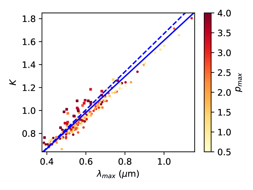
Figure 4: The Wilking relation derived from our fits. Colored points correspond to the median values of the $K$ and $\lambda_{max}$ posterior distributions. Our obtained slope, $1.57^{0.31}_{-0.39}$, (solid line) is statistically consistent with previous constraints (dashed line). The colorbar shows $p_{max}$ for each measurement. Close to 0.5 $\mu$m  a group of points maximally deviates from the linear relation. These measurements have high $p_{max}$, and $K$ / $\lambda_{max}$ ratios, likely due to 3D effects or extreme alignment properties (Sect. 4.1), and lie close to the $p_{max}$ / $E(B-V)$ limit (Fig. 10).

We explored the correlations between $K$ and $\lambda_{max}$. Colored points in Fig. 4 show the median of the posterior distributions for sightlines with $\Delta\theta$ $\leq 1$, and $\chi^{2}\leq 1$. Uncertainties are not shown for vizualization purposes because the S/N ratio in the obtained $K$ values is low. This limitation arises from the existing polarization data, which only include a small number of measurements, preventing accurate constraints of the width of the Serkowksi relation. Spectropolarimetric data are required for this task, but their current availability is limited. Despite these limitations, exploring the variations and relationship between $K$, and $\lambda_{max}$ remains meaningful to motivate further studies.

We fit linear models to the data using an iterative method called ”random sample consensus”, as implemented in Python (Pedregosa et al., 2011). This method uses random sub-samples to estimate the model parameters that optimally fit the data, and is less sensitive to outliers than standard regression algorithms.

Similarly to past works (Wilking et al., 1980; Whittet et al., 1992), we find a linear correlation between $K$ and $\lambda_{max}$. This was expected because it was assumed in the distribution of priors (Sect. 3.1.2). Uncertainties were estimated through bootstrapping: fitting linear models to the data with $K$, and $\lambda_{max}$ randomly drawn from the posterior distributions. The median with its corresponding $68\%$ percentiles of the obtained coefficients of the fit is (blue solid line in Fig. 4)

$$K=1.58^{+0.36}_{-0.37}\leavevmode\nobreak\ \lambda_{max}+0.04^{+0.19}_{-0.17}.$$ (16)

The intercept is consistent with zero, as shown before. The median value of the obtained slope is lower, but statistically consistent, within one sigma, with previous constraints.

Existing constraints on the Wilking relation slope have been obtained for $\lambda_{max}$ $\lesssim 0.8$ $\mu$m, because measurements with $\lambda_{max}$ $>0.8$ $\mu$m had variable EVPAs (Whittet et al., 1992). We have excluded variable measurements from our sample, but several points with $\lambda_{max}$ $>0.8$ $\mu$m remained. It is mainly those points that drive our obtained slopes to lower values. This suggests that the intrinsic slope in the Wilking relation might be lower than previously thought. Our statistical uncertainties do not allow us to draw any significant conclusions. High accuracy observations with $\lambda_{max}$ $\gtrsim 0.8$ $\mu$m could shed light on potential shifts to the intrinsic slope between $\lambda_{max}$ and $K$.

Fig. 4 includes several points with nominal $\lambda_{max}$, around 0.55 $\mu$m, but higher $K$ than the Wilking relation predicts, implying narrower $p_{\lambda}$ profiles. These points tends have a relatively high degree of polarization, $p_{max}$ $\gtrsim 2.5\%$ (for example, third row in Fig. 1). Measurements that maximally deviate from the Wilking relation correspond to approximately $8\%$ of the sample. We identified those measurements using the following criteria: 1) $\lambda_{max}$ $\approx 0.55$ $\mu$m; 2) $K$ / $\lambda_{max}$ $\gtrsim$ 1.75. For normal stars, $K$ / $\lambda_{max}$ is derived from the standard Wilking relation slope (Eq. 2).

We note that the S/N ratio in $p$ of these (deviating) measurements is high, because $p_{max}$ is maximum there; thus, these fits are among the best we obtained. The obtained constraints, however, are not equally well for all three free parameters (Fig. 3), mainly due to the lack of near-UV, -IR polarization measurements (Sect. 3.1.2). For these reasons, we tested if the presence of these deviating measurements can be attributed to some statistical (observational or instrumental) bias.

Firstly, we confirmed that the measurements of stars deviating from the Wilking relation were obtained from various authors (Vaillancourt et al., 2020; Weitenbeck, 2008; Andersson & Potter, 2010; Eswaraiah et al., 2012), and different instruments: HIPPO, (Potter et al., 2008), HPOL (Wolff et al., 1996), TURPOL (Piirola, 1988), AIMPOL (Rautela et al., 2004). Thus, no instrumental bias could explain the observed trend.

We performed Monte Carlo simulations to test for statistical biases induced by observational uncertainties. We created mock samples by randomly drawing values from the $\lambda_{max}$, and $K$ posterior distributions of these deviating points. We found that there is always a non-zero fraction of points that deviates from the Wilking relation. To quantify the probabilities of this effect, we constructed the distribution of relative fractions of deviating points with respect to the total number of measurements each mock sample has. The median of the distribution is $5\%$, while the $99.9\%$ confidence interval is $2-6.7\%$. This test confirms that deviating points were not occurred by chance, and are always present despite large uncertainties. Omitting those measurements in the fitting process does not affect the obtained constraints of the Wilking relation (Eq. 16).

Sightlines with high $K$ have been previously reported (Weitenbeck, 2008; Patat et al., 2015), although no clue about their origin exists yet. We found evidence that LOS integration effects or enhanced grain alignment efficiency could explain this trend (Sects. 4.1, and 6.1).

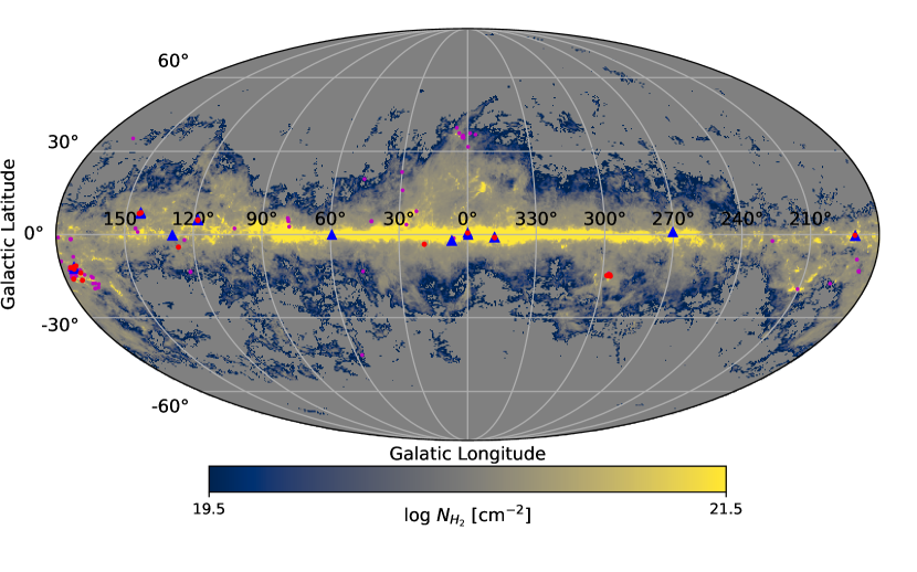
Figure 5: The target sightlines overplotted on a full-sky molecular column density map of our Galaxy (Skalidis et al., 2024). Sightlines with typical $\lambda_{max}$ are shown as magenta points. These measurements are primarily encountered in diffuse molecular clouds. Blue triangles show sightlines that follow the Wilking relation, and have $p_{max}$ $>3\%$; all of them are in the Galactic plane. Red dots correspond to stars that deviate from the Wilking relation, and usually have high $p_{max}$. Deviating measurements are always found in LOSs with significant molecular hydrogen column densities, and detectable CO intensities (higher than 1 K km s^-1).

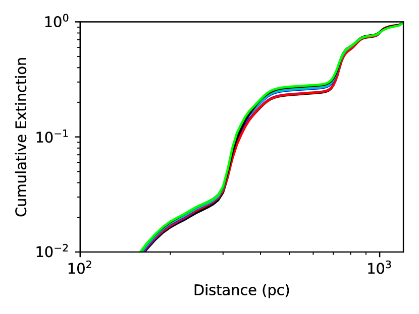
Figure 6: Cumulative extinction, obtained from Edenhofer et al. (2024), versus distances towards the Berkeley 59 star cluster, which is located at $\sim 1$ kpc. Colored curves correspond to different LOSs. Extinction steeply rises from 0.2 to 1.0 kpc. Polarization data suggests that there is significant dust column beyond 1 kpc (Fig. 7), but the distance limit of the employed 3D extinction map does not allow us to confidently explore this.

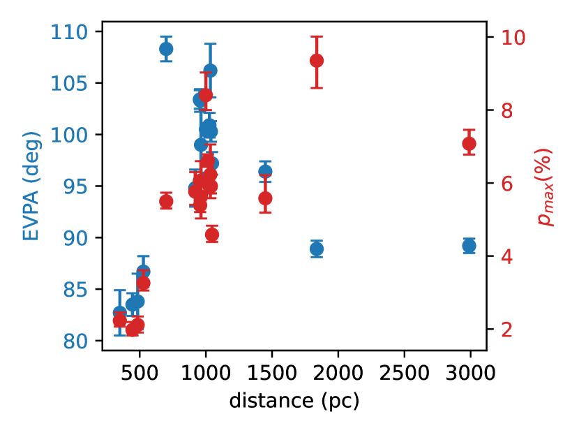
Figure 7: EVPA (blue, left vertical axis), and $p_{max}$ (red, right vertical axis) as a function of distance toward the Berkeley 59 cluster.

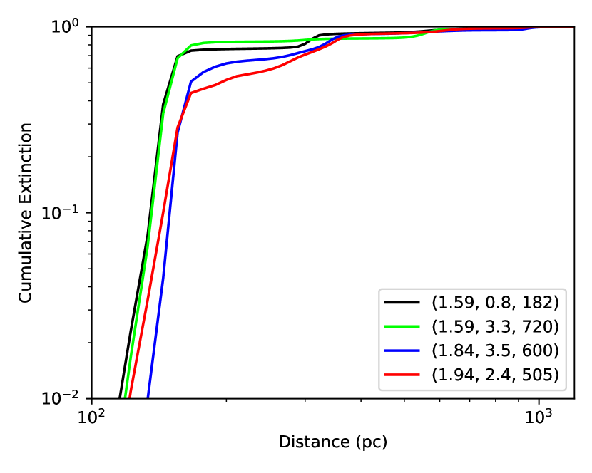
Figure 8: Cumulative extinction, obtained from Edenhofer et al. (2024), versus distance toward four different LOSs in the Taurus molecular cloud complex. Colored lines corresponds to measurements with different polarization properties. The legend shows $K$ / $\lambda_{max}$, $p_{max}$, and the distance of each star. Sightlines with nominal $K$ / $\lambda_{max}$, which is approximately equal to 1.66 (black, and lime curves), have a dominant peak at 150 pc, which corresponds to the Taurus molecular distance. Sightlines with maximum $K$/ $\lambda_{max}$ (blue, and red curves) show significant contribution from the Perseus molecular cloud, which is located at 300 pc. These results indicate that LOS integration effects can enhance $K$ without suppressing $p_{max}$, hence the polarization contribution of the two clouds acts constructively; this implies that the magnetic field remains nearly uniform along these LOSs.

4.1 Observational evidence of high $K$ due to 3D effects and enhanced grain alignment

Measurements that follow the Wilking relation are randomly distributed in our Galaxy (Fig. 5), and stars with $p_{max}$ $\geq 3\%$ tend to be along the Galactic plane. Stars that deviate from the Wilking relation are distributed around the Galactic plane; towards molecular clouds traceable by the CO (J=1-0) emission line (Skalidis et al., 2024). The majority of these (deviating) measurements are towards the Taurus and, the Chameleon I molecular clouds and the cluster Berkeley 59. We examined the characteristics of the aforementioned regions to identify the potential origin of their enhanced $K$ / $\lambda_{max}$.

4.1.1 Berkeley 59

The young open cluster Berkeley 59 is centered at RA, Dec = 0.543333$\degr$, +67.419444$\degr$ with a radius approximately equal to $10\arcmin$. The cluster lies at $\sim 1$ kpc, and three foreground dust layers with different magnetic field geometries contribute to the starlight polarization along this LOS (Eswaraiah et al., 2012). We explored dust extinction variations with distance using a 3D dust extinction map (Edenhofer et al., 2024), and, when necessary, we employed stellar distances from the catalogue of Bailer-Jones et al. (2021), which uses parallaxes from the Gaia early data release 3 (Gaia Collaboration et al., 2021).

Fig. 6 shows several cumulative extinction profiles towards the Berkeley 59 cluster. The three dust layers identified by Eswaraiah et al. (2012) at approximately 300, 500, and 700 pc are prominent in the depicted extinction curves. The cumulative extinction is $\gtrsim 90\%$ at 1 kpc, implying that most of the dust column is within this distance. However, a significant dust column might be beyond 1 kpc – this is not surprising because the cluster is close to the Galactic plane – but the employed 3D extinction map is limited to 1.2 kpc. Another map (Green et al., 2018) suggests a $\sim 7\%$ increment in the dust reddening from 1 to 3 kpc.

Starlight polarization is a powerful tool for studying LOS integration effects due to dust structure, and magnetic field variations (Tassis et al., 2018; Panopoulou et al., 2019b; Pelgrims et al., 2023, 2024; Mandarakas et al., 2024). We explored how $p_{max}$, and EVPA changes with distance (Fig. 7). The degree of polarization is around $2\%$ at 500 pc with an average EVPA approximately $82\degr$. At 1 kpc, $p_{max}$ $\approx 6\%$, and EVPA$\approx 95\%$. Beyond this distance, the cluster dominates in extinction and polarization.

For distances larger than 1 kpc, $p_{max}$ remains nearly flat, but EVPAs significantly change. The average EVPA of Berkeley 59 is close to $95\degr$, but the EVPAs of the two most distant measurements (located at 1.6, and 3.0 kpc respectively) are 90$\degr$, and 88$\degr$ respectively. Given the uncertainties, which are close to $1\degr$, this difference is statistically significant, and it implies that the magnetic field orientation beyond the cluster changes with distance by almost $5\degr$. The two most distant measurements have relatively high $K$ / $\lambda_{max}$ ratios, close to 1.78, and 1.81 respectively; thus, they deviate from the Wilking relation. The average $K$ / $\lambda_{max}$ of the cluster is 1.65, which is consistent with the Wilking relation. This suggests that LOS variations of the magnetic can bias $K$ / $\lambda_{max}$ to larger values, although $p_{max}$ is not significantly suppressed.

LOS integration effects are thought to act destructively in polarization (e.g., Angarita et al., 2023). This is expected when clouds have different magnetic field geometries along the LOS or the magnetic field is inclined with respect to the plane of the sky (POS). Mandarakas et al. (2024) found some regions where integration effects likely act constructively, which can only happen if magnetic field orientations remain constant with distance. Towards the Berkeley 59 LOS, EVPA weakly changes after 1 kpc (Fig. 7), which implies that depolarization effects are minor, and that the POS magnetic field morphology remains coherent for at least 2.0 kpc.

4.1.2 Chameleon I

A large fraction of the data showing maximum $p_{max}$, and $K$ / $\lambda_{max}$ are located in the star-forming molecular cloud Chameleon I. The distance of this cloud is around $160\pm 15$ pc (Whittet et al., 1997). A 3D dust extinction map (Edenhofer et al., 2024) confirms this estimate, and also suggests that it is the dominant structure along this LOS (not shown here). For this reason, 3D integration effects have no contribution to the observed starlight polarization there.

Andersson & Potter (2010) obtained multi-band polarization data around the young stellar object (YSO) HD 97300, which is in Chameleon I. They found that the polarization efficiency is maximized around the YSO, primarily due to its anisotropic and intense radiation field, as expected from the radiative alignment theory (RAT, Lazarian & Hoang, 2007). They did not attempt to include $K$ as a free parameter in their Serkowski fits, but instead they assumed a Wilking relation with a well-defined slope. For this reason, no published $K$ constraints of this dataset exist.

Our employed approach allows us to constrain $K$, although at the cost of getting larger uncertainties in the obtained posterior distributions. We found that all stars but one lying within $\sim 0.5\degr$ away from the target YSO have high $K$ / $\lambda_{max}$  ratios, approximately ranging from 1.7 to 2. As Andersson & Potter (2010) mentioned, radiation heating of grains by the YSO is effective up to $0.75\degr$ there, which sets a rough upper limit in the maximum distance the YSO radiation field can impact dust alignment. Therefore, polarization measurements have maximum alignment efficiency, likely due to their proximity to the YSO. Assuming a standard (aligned) dust grain size distribution with a well defined mean, hence $\lambda_{max}$, maximum alignment efficiency would yield higher $p_{max}$, hence higher $K$ because the Serkowski relation becomes narrower.

There is only one star close ($\sim 20\arcmin$) to the YSO that follows the Wilking relation, but it is located at 2 kpc, which is beyond what the employed 3D extinction map covers (Edenhofer et al., 2024); the map of Green et al. (2018) has no coverage of this region. Thus, some background cloud could have affected the polarization of this star. All the other nearby measurements are within 1 kpc, where according to the 3D extinction map the Chameleon I structure dominates, and deviate from the Wilking relation. All this evidence suggests that regions with maximum polarization efficiency could lead to deviations from the Wilking relation.

4.1.3 The Taurus molecular cloud complex

The Taurus star-forming region is a nearby ($\sim 150$ pc) extended molecular cloud complex with an estimated median depth around 25 pc (Galli et al., 2019). The nearest structure of the Taurus complex is approximately located at 128 pc, while the furthest structure is at 198 pc (Fig. 8). The magnetic field properties of the Taurus complex have been thoroughly studied (Goldsmith et al., 2008; Heyer et al., 2008; Chapman et al., 2011; Tritsis et al., 2018).

Vaillancourt et al. (2020) studied the dust grain properties of the Taurus complex with multi-band polarization data. They found that dust grains grow in high-density clumps, likely due to coagulation. They also confirmed the validity of the previously established linear relationship between $\lambda_{max}$ and $A_{V}$ (Andersson & Potter, 2007), which can be understood in the context of the RAT alignment theory.

Per the RAT theory, ISM dust grains align with the magnetic field due to radiation torques induced by anisotropic radiation fields. Photons with wavelengths significantly larger than the size of grains, weakly interact with the grains. Thus, the minimum grain size sets the maximum wavelength of the incident radiation that couples to dust grains. As the minimum grain size increases, longer wavelengths can perturb the grains. At higher extinctions, radiation becomes redder, and hence the minimum grain size that can interact with the penetrating radiation, hence align with the magnetic field, increases. Considering that $\lambda_{max}$ is proportional to the minimum grain size (Mathis, 1986), a correlation between $\lambda_{max}$, and $A_{V}$ naturally emerges from this theory.

Vaillancourt et al. (2020) verified that the linear relationship between $\lambda_{max}$ and $A_{V}$ applies up to $A_{V}$ $\approx 10$ mag. However, they found that the $\lambda_{max}$ - $A_{V}$ bifurcates for $A_{V}$ $\gtrsim 1.5$. By modeling the data, they concluded that bifurcation can be explained if both grains are larger, and small grains are weakly aligned there, which primarily happens due to dust-gas collisions whose frequency increases with density (Hoang et al., 2015).

We confirmed that our high-$K$ measurements are consistent with a typical $\lambda_{max}$ – $A_{V}$ linear relation (Andersson & Potter, 2007). We found no association between measurements that deviate from the Wilking relation (this work), and measurements that bifurcate in the $\lambda_{max}$ – $A_{V}$ linear relation (Vaillancourt et al., 2020). We found that LOS integration effects are likely responsible for the observed high $K$ values in the Taurus molecular cloud complex.

Fig. 8 shows the cumulative dust extinction profiles with distance towards several LOS in the Taurus molecular cloud complex. All extinction profiles show a steep rise at 150 pc, which corresponds to the distance of the Taurus molecular cloud complex. However, for some sightlines (shown with the blue and red curves in Fig. 8) there is a significant contribution to the total dust extinction ($\sim 50\%$) from background structures; this is evident by a constant rise in some of the extinction curves for distances greater than $200$ pc.

3D dust mapping techniques suggest that the Taurus complex is located at the nearest edge of a giant shell that was formed by a supernova (Bialy et al., 2021). Another well-studied molecular cloud sits at the furthest edge of the same shell: the Perseus molecular cloud. Thus, the increase that we observe in the extinction at large distances (Fig. 8) is due to the Perseus molecular cloud, which sits at the other edge of the bubble at a distance close to 300 pc (Zucker et al., 2021).

Measurements with high $K$ / $\lambda_{max}$, and $p_{max}$, which deviate from the Wilking relation, are located behind both the Taurus, and the Perseus molecular clouds (distances greater than 300 pc). For sightlines where the Perseus molecular cloud has minimum contribution to the total dust extinction (green, and black curves in Fig. 8), polarization measurements show typical $K$ / $\lambda_{max}$ values. Thus, similarly to the Berkeley 59 (Sect. 4.1.1), we found that LOS integration effects can lead to deviations from the Wilking relation.

The fact that $p_{max}$ does not decrease even when both clouds contribute to starlight polarization (legends in Fig. 8 show $p_{max}$ and the distances of the stars), implies that the POS morphology of the magnetic field in both clouds is comparable. This suggests that the initial magnetic field of the bubble has been uniformly pushed by the expanding gas, which complies with a nearly spherical shape for the shell.

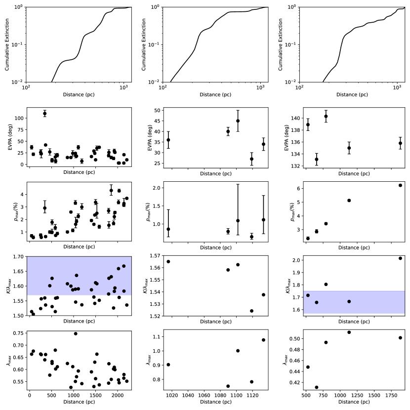
Figure 9: Variations in dust extinction and polarization properties as a function of the distance of several stars. The left, middle, and right columns correspond to measurements toward the star clusters NGC 6823, 6709, and 1502, respectively. Shaded regions in the K / $\lambda_{max}$ profiles show the one sigma confidence intervals (Eq. 2). The observed variance in K / $\lambda_{max}$ is due to LOS variations in the magnetic field morphology. LOS integration effects tend to bias $\lambda_{max}$ to smaller values, hence K / $\lambda_{max}$ to larger values.

4.2 Stars following the Wilking relation: 3D effects are still important

We showed that LOS integration effects are likely responsible for the non-linear increase of $K$ with respect to $\lambda_{max}$. Here, we wish to answer the following question: Are integration effects negligible when polarization measurements follow the Wilking relation? Below we show some characteristic examples demonstrating that even if the Wilking relation applies, 3D effects can still be important.

The first example is the NGC 6823 young open cluster, which is located at RA, Dec = $295.787574\degr$, $23.300126\degr$, and is close to 2 kpc (Guetter, 1992). Medhi et al. (2010) obtained multi-wavelength polarization data toward this cluster and found that several foreground dust layers contribute to the observed polarization, which is consistent with 3D dust extinction maps (top left panel in Fig. 9)

Left column in Fig. 9 shows the variance of dust extinction, and polarization properties of several stars at different distances toward the target cluster. We observe that EVPA weakly decreases with distance, which suggests that the magnetic field orientation remains coherent over several hundreds of pc. This is also evident in the $p_{max}$ versus distance profile, where $p_{max}$ increases from $0.5\%$ at 0.1 kpc to $4\%$ 1 kpc. The increase of $p_{max}$ implies that LOS integration effects act constructively here, leading to high $p_{max}$ values. $K$ / $\lambda_{max}$ ratio shows evidence of a weak correlation with distance, while a more prominent anti-correlation between $\lambda_{max}$ and stellar distance appears.

In this region, $K$ / $\lambda_{max}$ increases but the values are consistent with the constraints of the Wilking slope. $K$ / $\lambda_{max}$ of the nearest star, whose data better resembles the intrinsic dust properties because integration effects are minimum, is equal to 1.50, which is more than a sigma lower than the standard Wilking relation slope. This happens because for this star $\lambda_{max}$ $\approx 0.66$ $\mu$m, which is higher than typical values ($\lambda_{max}$ = 0.55 $\mu$m). Thus, LOS integration effects seem to bias $\lambda_{max}$ to lower values, hence $K$ / $\lambda_{max}$ to larger values. This is further supported by Fig. 12.

Fig. 9 shows two more characteristic regions. The third column of Fig. 9 shows data from Weitenbeck (2008) toward the open cluster NGC 1502, which is located at around 1 kpc. The extinction profile rapidly increases at $\sim 250$ pc, and from 300 pc to 1 kpc, dust extinction increases with a nearly constant rate. This implies that there are several foreground structures, which are also evident in the EVPA, and $p_{max}$ versus distance profiles. For the farthest star, $K$ / $\lambda_{max}$ is significantly higher than standard values due to LOS integration effects, similar to other regions (Sects. 4.1.1, and 4.1.3).

The middle column of Fig. 9 shows data from Topasna et al. (2022) toward the NGC 6709 open cluster. This cluster lies at $\sim 1$ kpc and the extinction curve shows that there are several foreground structures. Data availability is limited there, but we observe a weak anti-correlation between $K$ / $\lambda_{max}$ with distance. The decrease of $K$ / $\lambda_{max}$ is not as prominent as in other cases, but it is the only region showing evidence of suppression in the values of $K$ / $\lambda_{max}$ due to integration effects.

We conclude that LOS variations in the magnetic field morphology can be significant in both measurements following or deviating from the Wilking relation. The previously reported cosmic variance in the slopes of the Wilking relation (Whittet et al., 1992) can be attribute to LOS averaging effects. The observed correlations between $K$ / $\lambda_{max}$, and $\lambda_{max}$ with stellar distances suggests that the obtained values are significantly contaminated by averaging effects, hence do not accurately probe the dust grain properties. LOS integration effects bias the obtained Serkoski parameters. As noted by Mandarakas et al. (2024), the majority of LOSs in the compiled catalogue (Panopoulou et al., 2023) include multiple clouds along a LOS. Thus, existing constraints on the Serkowski parameters are biased due to projection effects. The only secure way that guarantees the absence of 3D effects in the obtained Serkowski fits is the parallel examination of dust extinction and polarization profiles with distance. A caveat of our analysis is that the extinction curves vary within each region, and this explains the significant spread in the observed trends of Fig. 9.

5 Polarization efficiency

Polarization efficiency, represented as $p_{max}$ / $E(B-V)$, quantifies the ability of aligned dust grains to polarize starlight and provides a crucial constraint for dust grain models (Hensley & Draine, 2021). Complex magnetic field topologies, especially when the field is inclined with respect to the LOS, can reduce the observed $p_{max}$ values (e.g., Angarita et al., 2023), which is why only the upper limits of $p_{max}$ / $E(B-V)$ probe the intrinsic polarization efficiency of interstellar grains.

The upper limit in $p$ / $E(B-V)$ was initially estimated around $9\%$ (Serkowski et al., 1975). However, in several diffuse ISM regions with $E(B-V)$ $\sim 0.01$ mag, this limit was systematically exceeded (Skalidis et al., 2018; Panopoulou et al., 2019a; Angarita et al., 2023), suggesting that previous constraints underestimate the true alignment efficiency of ISM grains. Polarized dust emission data from the Planck satellite yielded a higher polarization efficiency, $p_{max}$ / $E(B-V)$ $=13\%$ (Planck Collaboration et al., 2020a).

We examined the polarization efficiencies in our sample. Fig. 10 shows $p_{max}$ versus $E(B-V)$ and the corresponding upper limits. $E(B-V)$ is computed up to the distance of the star with the use of a 3D extinction map (Green et al., 2018), and stellar distances from Gaia (Gaia Collaboration et al., 2021).

The vast majority of our data is bounded by the revised limit, $p$ / $E(B-V)$ $=13\%$, hence our results are consistent with Planck Collaboration et al. (2020a). Uncertainties in the extinction maps limit our ability to constrain polarization efficiencies (Panopoulou et al., 2019a). Therefore, we consider the observed violations of the $13\%$ limit statistically insignificant. We note, however, that polarization efficiencies as high as $15.8\%$ have been reported in the diffuse ISM (Angarita et al., 2023), which implies that the $13\%$ upper limit might actually be underestimated. Measurements with maximum $K$ / $\lambda_{max}$ ratios, which deviate from the Wilking relation, tend to have relatively high polarization efficiencies (red stars in Fig. 10), which is consistent with our results about the constructive contribution of LOS integration effects towards these sightlines (Sect. 4).

A notable transition in polarization efficiencies occurs at $E(B-V)$ $\approx 0.5$ mag. For $E(B-V)$ $\lesssim 0.5$ mag, measurements are bounded by the $13\%$ limit, while for $E(B-V)$ $\gtrsim 0.5$ mag all measurements are bounded by the $9\%$ limit. This transition in polarization efficiencies could be explained by the following scenarios, which are expected in high extinction regions: 1) loss of alignment because of the reddening of the incident radiation, which causes only large grains to align; 2) the average grain size increases at high densities, hence small grains are less abundant there; 3) variations in the grain composition; 4) projection effects.

If we consider that $N_{H}$ / $E(B-V)$ $=5.8\times 10^{21}$ cm^-2 (Bohlin et al., 1978), which applies for $E(B-V)$ $\gtrsim 0.1$ mag (Skalidis et al., 2024), we obtain that $N_{H}\sim 3\times 10^{21}$ cm^-2; this value marks the onset of the fully molecular hydrogen regime (Bellomi et al., 2020). The observed decrease in polarization efficiencies seems to correlate with the presence of molecular gas. However, we found compelling evidence that the observed trend is induced by projection effects, which are more prominent in molecular sightlines (Skalidis et al., 2024).

For $E(B-V)$ $\gtrsim 0.3$ mag, the probability of having multiple clouds along a LOS increases (Skalidis et al., 2024). Depolarization effects due to LOS magnetic field orientation variations, which only reduce $p_{max}$, are more likely to happen in LOSs with multiple clouds. We have seen that integration effects can act constructively, hence increase $p_{max}$ (Sect. 4). However, even a slight difference in the magnetic field morphologies of two clouds along the same LOS would suppress $p_{max}$ from reaching its maximum value.

The contribution of projection effects to $p_{max}$ / $E(B-V)$ is evident in Fig. 11, which shows the cumulative median profile of $p_{max}$ / $E(B-V)$ with distance. The suppression of the median $p_{max}$ / $E(B-V)$ with distance strongly suggests that the observed transition in Fig. 10 is due to the presence of multiple clouds, and thus it is unrelated to grain alignment physics; if the suppression of $p_{max}$ / $E(B-V)$ was merely due to loss of grain alignment, it should be independent of stellar distance. This limits our ability to constrain grain alignment theories with this observable and questions some of the existing results (Andersson et al., 2015).

We found similar trends for the other two Serkowski parameters: $\lambda_{max}$, and $K$. Fig. 11 shows the cumulative median profiles of $\lambda_{max}$, and $K$ with $E(B-V)$. Each point in the curves corresponds to the median value of points with dust reddening lower than the depicted values. For $E(B-V)$ $<0.5$ mag, the median values of $\lambda_{max}$, and $K$ are greater than existing constraints (Whittet et al., 1992), while for $E(B-V)$ $\gtrsim 0.5$ mag, both medians progressively converge to past values. Here $\lambda_{max}$ seems to anti-correlate with $E(B-V)$, which is the opposite of what the RAT theory predicts, and was found by Andersson & Potter (2007). This further supports that the observed suppression in the polarization efficiency (Fig. 10) is unrelated to grain alignment physics.

Our results indicate that LOS integration effects tend to bias both $\lambda_{max}$, and $K$. Considering that low-extinction sightlines have fewer clouds, the obtained constraints in regions with $E(B-V)$ $\gtrsim 0.5$ mag should better resemble the intrinsic properties of aligned dust. In these regions, the average $\lambda_{max}$, and $K$ are equal to 0.63 $\mu$m, and 1.0 respectively (Fig. 12), which implies that the Wilking relation slope should be $\sim 1.58$, consistent with our obtained slope (Eq. 16). For LOSs with $E(B-V)$ $<$ 0.2 mag, the distribution of $\lambda_{max}$ becomes bimodal with the two modes located at 0.4 $\mu$m and 0.6 $\mu$m respectively. A similar result, although with slightly offset modes, was found by Mandarakas et al. (2024) toward LOSs with one dominant cloud. This suggests that: 1) low extinction sightlines are less susceptible to LOS integration effects because the expected number of clouds is close to unity, and 2) the intrinsic distribution of $\lambda_{max}$ might be bimodal. Further investigation is required to explore this.

For $E(B-V)$ $\gtrsim 0.5$ mag, which corresponds to molecular sightlines, the probability of having multiple clouds along the LOS is enhanced (Skalidis et al., 2024). In these LOSs, both $\lambda_{max}$, and $K$ are lower, and equal to $\lambda_{max}$ $\approx 0.55$ $\mu$m, and $K\approx 0.9$, than the diffuse ISM values, due to projection effects. We conclude that the Serkowski parameters, which are free from projection effects, related to the intrinsic dust properties should be $10\%$ off from previous constraints. The intrinsic distributions of $K$, and $\lambda_{max}$ might differ from existing constraints.

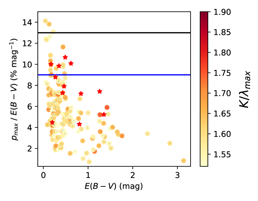
Figure 10: Maximum polarization fraction, obtained from our fits, versus dust reddening. The black, and blue lines correspond to the $13\%$, and $9\%$ upper limits respectively. Colorbar shows our obtained Wilking relation slopes. Points with high $K$/$\lambda_{max}$ (red stars) tend to have maximum polarization efficiencies. Polarization efficiencies decrease from $13\%$ to $9\%$ at $E(B-V)$ $\approx 0.5$ mag due to LOS effects.

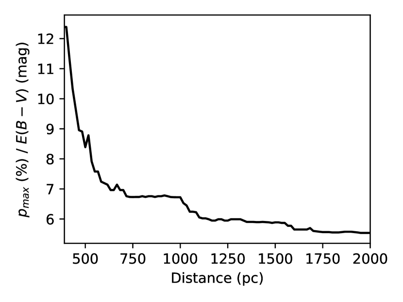
Figure 11: Cumulative polarization efficiency with distance. The decrease in polarization efficiency with distance strongly suggests that the observed reduction of $p_{max}$ / $E(B-V)$ at $E(B-V)$ ¿ 0.5 mag (Fig. 10) comes from the contribution of multiple clouds along the high extinction LOSs. In these cases, $p_{max}$ / $E(B-V)$ is a poor tracer of grain alignment efficiency.

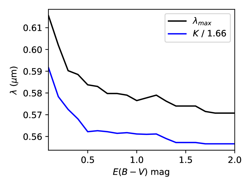
Figure 12: Cumulative median profiles of $\lambda_{max}$, and $K$ with $E(B-V)$. $K$ has been normalized with the value of the Wilking slope for vizualization purposes. For $E(B-V)$ $\lesssim 0.5$ mag, the average $\lambda_{max}$ $\approx 0.63$ $\mu$m, while the average $K\approx 1.0$. Both averages are slightly higher than previous constraints, which are $\lambda_{max}$ $\approx 0.55$ $\mu$m, and $K\approx 0.9$. For $E(B-V)$ $>0.5$ mag, integration effects are more prominent and both $\lambda_{max}$, and $K$ progressively converge to the previously reported Galactic averages.

6 Discussion

6.1 The Wilking relation: reconciling theory with observations

The dependence of the degree of polarization with wavelength can be viewed as the contribution of multiple grain sizes (Mathis, 1986). If the polarization signal was only induced by a single-size population, then the $p(\lambda)$ profiles should approximate a delta function. Thus, the broadening in the $p(\lambda)$ curves reflects the range of aligned grain sizes, even if this range is narrow.

Regions with large grains have high $\lambda_{max}$ because $\lambda_{max}$ is proportional to the minimum, hence to the average, grain size (Mathis, 1986). If we assume an MRN-like grain size distribution, and a constant total dust mass, any increase in the minimum grain size limit, which can be due to a depletion of small grains, will decrease $\lambda_{max}$. If the maximum grain size limit remains roughly constant during this grain growth process (Voshchinnikov & Hirashita, 2014; Andersson et al., 2015), then the difference between the minimum and maximum aligned grain size would increase, implying a narrower $p(\lambda)$ profile; hence a larger $K$. In this picture, a causal relationship between $\lambda_{max}$ and $K$ (Wilking relation) naturally emerges.

We found several measurements whose $K$ values were higher than predicted from the Wilking relation (Eq. 16). To understand this, we shall hypothesize two regions with the same grain size distributions, hence $\lambda_{max}$, but different alignment efficiencies. The region with higher alignment efficiency should have a higher $p_{max}$. Keeping the grain size distribution constant but increasing $p_{max}$ yields a narrower (high $K$) Serkowski profile. Measurements around the YSO in the Chameleon I molecular cloud (Andersson & Potter, 2010) seem to be consistent with this scenario.

We expect that for each $\lambda_{max}$ there is a range of $K$ probing environments with different alignment efficiencies or grain properties. Dust grain growth models suggest that grain evolution could lead to linear relations between $\lambda_{max}$ and $K$ with different slopes (Voshchinnikov & Hirashita, 2014). Therefore, measurements that deviate from the standard Wilking relation ($K$ / $\lambda_{max}$ $\approx 1.66$) might have a different scaling because they correspond to larger grains.

In the Taurus molecular cloud, which we examined (Sect 4.1.3), Vaillancourt et al. (2020) suggested that the observed bifurcation in the $\lambda_{max}$ - $A_{V}$ relation is induced by large grains (Sect. 4.1.3). If there were a causal relation between grain growth and high $K$, we would expect to find deviations from the Wilking relation towards these bifurcated LOS, but we did not find so. However, the 3D magnetic field morphology, and dust structure of the Taurus molecular cloud are complex, and were not considered in the analysis of Vaillancourt et al. (2020). This might explain the discrepancy.

The majority of our obtained Serkowski parameters are contaminated by LOS integration effects. This happens for both measurements deviating or following the Wilking relation. Projection effects tend to bias $K$ / $\lambda_{max}$ to higher values (Sect. 4). If we assume that polarization measurements of nearby stars accurately probe the intrinsic dust properties, then our results suggest that $K$ / $\lambda_{max}$ $\sim 1.55$, which is smaller than the previously reported slope of the Wilking relation. In addition, considering low-extinction sightlines, where the number of LOS clouds is expected to be lower, we found that the average $\lambda_{max}$, and $K$ should be close to 0.63 $\mu$m, and 1.0 respectively; both are $\sim 10\%$ off from current constraints (Sect. 5).

7 Conclusions

The (empirical) Serkowski relation has been heavily used to constrain the properties of (aligned) ISM grains with multi-wavelength optical polarization data. Recently, Mandarakas et al. (2024) showed that the 3D structure of dust, and magnetic fields can significantly contaminate the constraints obtained by fitting the Serkowski relation to polarization data, hence limiting our ability to study grain physics.

Building on these recent advancements, we explored the intrinsic properties of aligned dust, with careful considerations of these 3D effects. Our findings indicate that even when standard conditions seem to hold, such as a constant EVPA and well-fitted Serkowski curves, 3D variations in magnetic field structure can still alter the obtained values, particularly through non-linear increases in $K$ (Sect. 4.1); this makes data deviate from the Wilking relation ($K$ / $\lambda_{max}$$>1.7$). Independent information obtained from 3D dust extinction maps supports this scenario.

We also found evidence that when the radiation field is enhanced, which according to the RAT theory should yield a maximum alignment efficacy between aspherical grains and magnetic fields, then the fits to the Serkowski relation also yield enhanced $K$ (Sect. 4.1.2). Thus, deviations from the Wilking relation can be induced by maximum alignment efficiencies. Limitations in the data availability lead to relatively low S/N ratios in the obtained fit parameters; hence further investigation is required to increase our confidence.

The vast majority of our obtained measurements follow the Wilking relation, despite LOS integration effects being significant. These cases can be only identified with the employment of 3D dust extinction maps. Projection effects tend to bias $\lambda_{max}$ to lower values, while $K$ to higher values, and can explain the cosmic variance about the linear slope between the two quantities. Focusing on regions where projection effects are minimal, we found that the Galactic median values for $\lambda_{max}$, and $K$ should be around 0.65 $\mu$m  and 1.0 respectively (Sect. 4.2). Both values are $10\%$ off from previous constraints, and suggest that the intrinsic $K$ / $\lambda_{max}$ $\sim 1.58$, which is smaller than the existing value (1.66, Eq. 2).

We explored the polarization efficiencies of our measurements, and found consistent results with past studies (Sect. 5). Some measurements exceeded the previously reported polarization efficiency limit, but this is statistically insignificant. For $E(B-V)$ $\lesssim 0.5$ mag, our data respect the existing maximum polarization efficiency, $p_{max}$ / $E(B-V)$= $13\%$, while for $E(B-V)$ $\approx 0.5$ mag, we found that measurements are bound by a lower limit, $p_{max}$ / $E(B-V)$= $9\%$.

The suppression of $p_{max}$ / $E(B-V)$ at high $E(B-V)$ has been previously observed in several molecular clouds, and was considered to be consistent with the RAT alignment theory. However, molecular sightlines have a larger number of LOS clouds (Skalidis et al., 2024), which leads to suppressing $p_{max}$ with respect to $E(B-V)$. This projection effect can sufficiently explain the observed suppression in $p_{max}$ / $E(B-V)$, which is unrelated to alignment efficiency. The observed decrease of the median $p_{max}$ / $E(B-V)$ with stellar distance (Fig. 11) further supports our thesis about the contribution of projection effects. These results call for further exploration because they challenge some of the existing observational constraints on grain alignment theories that are based on this observable. Similar results were reported by Planck Collaboration et al. (2020b).

Polarized thermal emission from ISM dust is more sensitive to projection effects than starlight polarization, because signal integration takes place along the entire LOS. This might hinder our ability to constrain grain properties, and alignment efficiency with this dataset (e.g., Ngoc et al., 2024); progress can be made with the parallel examination of dust polarization data and 3D dust extinction maps. Upcoming starlight polarization surveys, such as PASIPHAE (Tassis et al., 2018), aim to construct an atlas of the Galactic magnetic field in 3D, which is a necessary endeavor to derive robust constraints of grain properties.

Appendix A Polarization likelihoods

We demonstrate the properties of the polarization likelihoods at different S/N. We set the observational uncertainty equal to $\sigma=1\%$ and assumed different observed $p$ values. In this way, we control the S/N of the measurements as follows: for $p=0.1$ we obtain that S/N=0.1, while for $p=2$, we get that S/N=2.

Fig. 13 shows different normalized likelihood functions for S/N equal to 0.1 (green), 2 (blue), and 5 (black). Solid curves correspond to the total polarization likelihood that is a Rice distribution (Eq. 7, and Fig. 2 in Vaillancourt 2006). Dashed curves show the asymptotic expression of the polarization likelihood (Eq. 9), while dashed-dotted curves Gaussian profiles. For S/N=5, the different likelihoods are very close to each other, implying that the polarization likelihood approximates a Gaussian. However, the asymptotic likelihood has a slightly different amplitude than a Gaussian, which is also evident in Fig. 13 where the peak of the Gaussian (dashed-dotted black curve) is slightly shifted compared to the other two, which are nearly identical.

For S/N ¡ 3 (green and blue curves), both the Gaussian and the asymptotic likelihoods deviate from the polarization likelihood significantly. Overall, we found that the asymptotic form is accurate for S/N $\geq 4$, while a Gaussian for S/N $\geq 5$. We conclude that the asymptotic likelihood shown in Eq. (9) more accurately approximates the Rice distribution than a Gaussian at high S/N.

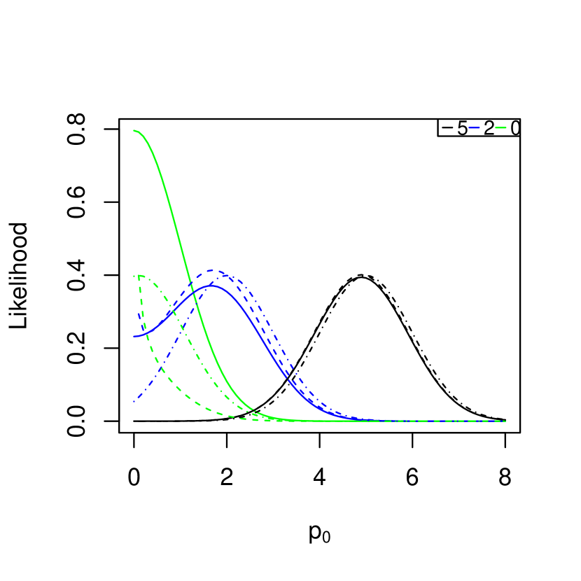
Figure 13: Normalized likelihood functions of the intrinsic (true or unbiased) polarization fraction for different S/N. Green curves correspond to S/N=0.1, while blue and black curves to S/N = 2, and 5 respectively, as shown in the legend. Solid, and dashed curves correspond to the total (Eq.7) and asymptotic (Eq. 9) polarization likelihoods, while dotted-dashed curves correspond to Gaussians. When S/N = 5, the asymptotic likelihood expression is nearly identical to the total likelihood.