Irreversibility of quantum field theory in de Sitter: the C, F and A theorems
Abstract
We prove the irreversibility of the renormalization group for quantum field theory in de Sitter space in , 3 and 4 space-time dimensions. The proof is based on strong subadditivity of the entanglement entropy, de Sitter invariance, and the Markov property of conformal field theory.
I Introduction
Understanding quantum field theory (QFT) in cosmological space-times is a fascinating open problem, as well as a necessary step towards formulating the physical laws in our universe. The interaction with a space-time dependent metric introduces phenomena that have no counterpart in flat space-time [1], and raises challenging problems related to cosmological horizons. In flat space, the renormalization group (RG) has provided a foundational framework to describe physics at different length scales in terms of flows of the couplings in the Hamiltonian [2]. However, the extension of RG methods to cosmological scenarios is less well developed and requires further exploration.
A key property of the RG in Minkowski space is that it is an irreversible process. This has been established in and space-time dimensions, leading to the C, F and A theorems, respectively [3, 4, 5, 6, 7]. These results have generated a rich interplay between unitarity and correlator methods, and results from quantum information theory. In this work, our goal is to establish the irreversibility of the RG for QFT in the simplest and most symmetric cosmological setting, the -dimensional de Sitter universe, . Recent progress in this direction has been achieved by [8, 9], who demonstrated the validity of the C-theorem in .
We prove that the information-theoretic approach of [6] can be generalized from Minkowski to de Sitter. Using strong subadditivity (SSA) of the entanglement entropy and de Sitter invariance, we derive the irreversibility formula
| (1) |
where is the difference of entanglement entropies between the UV fixed point and the QFT along the RG flow, evaluated on a causal diamond of radius inside the static patch of . The result has the same form as its Minkowski counterpart, while heavily relying on properties of . For our formula recovers the C-theorem; for it implies the F-theorem in ; and for it gives the A-theorem. These results provide new insights on nonperturbative QFT in de Sitter space, highlighting the utility of quantum information theory in cosmology.
II Setup
We consider unitary and de Sitter invariant quantum field theories (QFTs) in -dimensional de Sitter space-time, . In global conformal coordinates, the metric is
| (2) |
where is the radius, and the coordinate ranges , cover the full space-time. We focus on the space of QFTs that are obtained by perturbing a conformal field theory (CFT) by relevant scalar primary operators,
| (3) |
where the short distance scaling dimension of at the fixed point satisfies . The CFT acts as the ultraviolet fixed point for the QFT. We will work with the invariant Bunch-Davies or euclidean vacuum [10, 11, 12, 13]. The deformation (3) triggers a nontrivial renormalization group flow; correlation functions in the euclidean vacuum at a typical distance scale generally depend on and .
We will use the entanglement entropy to determine nonperturbative properties of RG flows in . Let us consider the vacuum entanglement entropy (EE) for a sphere of radius at (the neck of ), which we show on the Penrose diagram in Figure 1. The spatial entangling region is . The future boundary of the associated causal diamond in conformal coordinates is simply the null cone . When , the entangling radius becomes ; the entangling region covers the full static patch, and the EE becomes the thermal entropy. Since we are calculating the entanglement entropy with respect to a global pure state (the euclidean vacuum at ), the entropy of a region is equal to the entropy of its complement, which in this case gives . So the EE attains its maximum at , and for the EE coincides with that of a sphere inside the complementary static patch.
The EE for a QFT in is a divergent quantity; in general, it is a complicated function of the sphere radius , the radius , a short distance cutoff , and the relevant couplings in (3). We will be interested in the finite entropy difference
| (4) |
where is the entropy of the UV fixed point (plus appropriate local counterterms). We will analyze this subtraction procedure in more detail below.
In order to characterize the irreversibility of RG flows in , let us now describe the entropy for a CFT in . As we discuss in Sec. III, the existence of a conformal transformation between the causal diamond of a sphere in and that of a sphere in flat space, implies that the structure of the EE is the same as that in flat space:
| (7) | |||||
where the coefficients are proportional to inverse powers of the cutoff, . Our focus is on the quantities and , which are finite and intrinsic to the fixed point. They coincide with the corresponding and terms of the EE in flat space, and they can be computed as the universal terms of the free energy for a CFT on a sphere. is also the Euler anomaly in even , which for is proportional to the central charge of the CFT.
For a QFT in flat space, the UV fixed point can be probed in terms of the EE by taking , and the IR fixed point when . The irreversibility of the RG involves establishing that or decrease between the UV and IR fixed points. However, for a QFT in this notion needs to be generalized, because there is a maximum entangling distance scale , corresponding to the largest causally accessible region to an observer. Physically, the de Sitter temperature of the static patch limits the smallest energies that can be probed.
To extend the concept of irreversibility of the RG to we focus on EE inequalities. Building on the results of Secs. III and IV, we will demonstrate that (4) satisfies the irreversibility formula (1). Then we will define a running A-function (as well as analogous functions and ), and prove that these functions have to be negative for all unitary and de Sitter invariant QFTs. This construction provides a natural notion of irreversibility in in terms of finite physical quantities. At the maximum value , coincides with a thermal entropy difference, analogous to the Rindler limit in flat space. Furthermore, taking the limit recovers the results for Minkowski space.
III Entanglement and Markov property in
The derivation of the irreversibility formula for QFTs in de Sitter will rely on three ingredients: invariance, strong subadditivity (SSA) of the EE, and the Markov property for the CFT vacuum. This last property was proved in flat space in [14], and the goal of this section is to establish it in de Sitter.
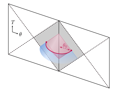
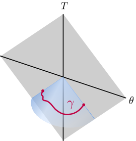
The setup we are interested in is that of entangling regions whose boundaries lie on the past light-cone from the origin, inside the static patch. In the proof of the irreversibility formula in Sec. IV, these boundaries will arise from applying a de Sitter boost to a spatial sphere. Consider a general curve on the past null cone from the origin inside the static patch of , as shown in Figure 2, parametrized by
| (8) |
which defines the boundary of some entangling region. Here is a unit vector describing the sphere . The metric (2) restricted to this null boundary describes a -dimensional sphere with varying radius
| (9) |
We want to determine the functional dependence of the EE for the CFT on a region with boundary on the null cone. This entropy is divergent, and we assume that it is regularized by a invariant cutoff (for instance using the mutual information [15]). Since the causal diamond is inside the static patch, we can compose the transformations of [16, 17] in order to conformally map this region onto a region with boundary on the null plane in flat space, (where are the remaining coordinates, and is a local function of ). If the CFT in this flat space has a Lorentz-invariant regularization, then the vacuum EE is independent of [18]. A simple way to see this is that is Lorentz invariant; under a Lorentz boost, , and taking we can transform the curved boundary into the Rindler edge. However, in general the invariant UV cutoff does not map to a Lorentz invariant cutoff in the flat space theory. This means that the EE can only depend on the boundary curve via the UV cutoff, and hence it has to be a local quantity on the boundary, up to an additive constant,
| (10) |
where is the unit radius sphere metric (see App. A for more details). This form for the EE satisfies
| (11) |
under null deformations of the boundary region, and the same for higher functional derivatives. This infinitesimal equality is equivalent to the formula
| (12) |
where and are finite regions with boundary on the null cone. In other words, strong subadditivity is saturated for the EE of a CFT with boundaries on the null cone in de Sitter. This is the Markov property for the CFT vacuum, which was proved in Minkowski in [14], and we now see that it is also valid in de Sitter. Eq. (11) will be important for the derivation of the irreversibility formula in the next section.
IV Irreversibility formula
Our goal now is to prove (1). The strategy is to use the isometries, reviewed in App. B, to deform the entangling region and derive a second order relation for the entanglement entropy. This, combined with SSA, will lead to the irreversibility formula. This approach was used in flat space in [19].
Consider a spatial sphere given by (8) with constant . The intrinsic radius is . Under a small boost of the curve, we can expand the EE in functional derivatives, and since the vacuum state is invariant, we arrive at
| (13) |
which gives, to every order in the boost parameter, an infinite hierarchy of equalities between derivatives of the EE. Here , we have denoted
| (14) |
and the angular integration is normalized such that . Note that
| (15) | ||||
Also, rotational invariance imposes some restrictions: has to be a constant and thus , and .
Under a boost in a direction , with boost parameter , it is not hard to check that the boundary curve is transformed to
| (16) |
See App. B for more details. Plugging this into (13), to first order on one obtains an equality which is automatically satisfied by rotational invariance. Meanwhile, at second order in we have two contributions: one from the first term in (13) keeping , and one from the second term keeping . The result is
| (17) | ||||
Rotational invariance allows to replace products such as inside integrals. Then (17) is equivalent to
| (18) |
where we have defined
| (19) |
Now we use strong subadditivity, which says that when the points do not coincide. This is not sufficient though, because the integral also receives a contribution from , and in this case the sign of is not determined. This is the step in which we use the Markov property. We construct the entropy difference
| (20) |
where is the entropy of the UV fixed point plus possible UV divergences induced by the relevant perturbations. This term is Markovian (the UV divergent terms are local on the entangling surface), and hence , and it vanishes at coincident points because the UV behavior of both terms is the same. Therefore,
| (21) |
Finally, recognizing that the second term here is , and replacing it in terms of using (18), we arrive at our main result
| (22) |
For , (22) shows that decreases along RG flows; in it implies the monotonic decrease of ; and for it establishes that . These quantities take the same form as their Minkowski counterparts. However, a key difference is that in flat space one can take , and these quantities become differences of IR and UV RG charges, while in the largest radius is restricted by the static patch size. Nevertheless, this generalized notion of irreversibility in de Sitter reduces to that of flat space in the limit of large radius. Additionally, in both de Sitter and flat space, the largest entangling region gives a thermal density matrix –Rindler in flat space, and the static patch in .
V Future directions
In this work, we used strong subadditivity of the EE and the Markov property of the CFT vacuum to establish the irreversibility of the renormalization group for general de Sitter invariant QFTs in , and dimensions. Our results show the promising role of quantum information theory methods in cosmology, and we would like to end by discussing some future directions.
In our approach, we kept the radius fixed and used the size of the entangling region to probe the RG, avoiding issues that can arise when relying on the thermal entropy instead [20]. It would be interesting to work out the thermal interpretation of our results in the limit when , likely connecting with recent developments in cosmological bootstrap techniques [21]. We expect that light-ray operators and energy conditions may also play a fruitful role in de Sitter. It would also be interesting to improve our nonperturbative understanding of entanglement in regions larger than the static patch, where time-dependence appears [22]. Developing numerical methods for evaluating the running C, F and A functions that we have defined in free massive QFTs would provide practical tools for further investigation [23, 24]. We are also currently analyzing the extension of our methods to AdS.
We thank H. Casini for discussions. NA is supported by a CONICET PhD fellowhip. GT is supported by CONICET (PIP grant 11220200101008CO), CNEA, and Instituto Balseiro, Universidad Nacional de Cuyo.
Appendix A Structure of the CFT vacuum EE on the light-cone
In this Appendix we will give a more explicit expression for the Markovian EE (10). It should be constructed using geometric quantities associated to the metric of (9), plus a possible anomaly term. The available geometric objects are the metric, it’s Riemann tensor, and the extrinsic curvatures. Since the space is conformally flat, the Riemann tensor can be obtained from the Ricci tensor. Furthermore, we will now show that the extrinsic curvatures can also be constructed from the induced metric and the Ricci tensor. We will set throughout this section.
The 2-dimensional vector space normal to the surface is generated by two null vectors:
| (23) | ||||
| (24) |
where is another null vector that satisfies . Then, the extrinsic curvatures are
| (25) |
Here is the projector onto the tangent space to the curve, namely
| (26) |
We note that the induced metric on the surface is given by , and its pullback on the tangent space is
| (27) |
where we have introduced the tangent vectors
| (28) |
We want to show that both extrinsic curvatures on the surface can be constructed using geometric quantities associated with .
After a few manipulations, one arrives at
| (29) |
and
| (30) |
One can write this now in terms of the unit sphere metric, transforming also the covariant derivatives. Then, using the relations between the Ricci tensors and curvatures associated with (which we will denote as and ) and [25], one can rewrite (A) in terms of intrinsic geometric quantities as
| (31) |
Furthermore, from the expressions (29) and (A), one can check that the invariant associated with the type B anomaly in the universal logarithmic term of the EE in [26] vanishes:
| (32) |
Let us now describe in more detail the Markovian expression for the CFT entanglement entropy. For odd there are no anomalous terms, and the most general expression for the local function is
| (33) |
On the other hand, for even we have to include a contribution that accounts for the Euler type A anomaly. Following [18], we can achieve this by including a Wess-Zumino term for the ‘dilaton field’ . In this reads
| (34) |
where the prefactor is fixed by the anomaly contribution for a sphere. Note that this term is a local functional of and , but not in terms of .
To sum up, let us explicitly write the surviving terms of the EE on the cone for a sphere with constant in and :
| (35) | ||||
| (36) |
Note that both expressions reduce to the well-known flat-space formulae in the limit .
Appendix B Infinitesimal deformations and dS invariance
In this Appendix we elaborate on some aspects of the symmetry group and focus on its infinitesimal action on spheres, as needed for the derivation of our irreversibility formula in Sec. IV.
It is convenient to perform this analysis in terms of the embedding of in a Minkowski spacetime as a hyperboloid of radius . Namely
| (37) |
where . Different parametrizations of the hyperboloid yield different coordinate systems on . Choosing
| (38) |
with , and describing a vector on the sphere , gives the global conformal coordinates with metric (2). The connected isometry group of can thus be obtained from the embedding, as the restriction of the Lorentz generators which preserve the hyperboloid. These are the generators of the group restricted to (37). Naturally, the Bunch-Davies vacuum is invariant under these isometries. In particular, the boosts preserve the light-cone through the origin , and we will be interested on using these generators to deform spatial spheres with boundary on the past cone.
Consider a boost of parameter along one direction acting on some spatial sphere given by . Its effect on a point on the sphere gives the relation
| (39) |
where . This parametrizes a boosted sphere with boundary on the cone. Writing , and plugging back into (39), we can solve for :
| (40) |
where . Finally, taking , we arrive at the formula for infinitesimal deformations
| (41) |
References
- [1] N. D. Birrell and P. C. W. Davies, Quantum Fields in Curved Space. Cambridge Monographs on Mathematical Physics. Cambridge University Press, Cambridge, UK, 1982.
- [2] K. G. Wilson and J. B. Kogut, “The Renormalization group and the epsilon expansion,” Phys. Rept. 12 (1974) 75–199.
- [3] A. B. Zamolodchikov, “Irreversibility of the Flux of the Renormalization Group in a 2D Field Theory,” JETP Lett. 43 (1986) 730–732. [Pisma Zh. Eksp. Teor. Fiz.43,565(1986)].
- [4] H. Casini and M. Huerta, “On the RG running of the entanglement entropy of a circle,” Phys. Rev. D85 (2012) 125016, arXiv:1202.5650 [hep-th].
- [5] Z. Komargodski and A. Schwimmer, “On Renormalization Group Flows in Four Dimensions,” JHEP 12 (2011) 099, arXiv:1107.3987 [hep-th].
- [6] H. Casini, E. Testé, and G. Torroba, “Markov Property of the Conformal Field Theory Vacuum and the a Theorem,” Phys. Rev. Lett. 118 no. 26, (2017) 261602, arXiv:1704.01870 [hep-th].
- [7] T. Hartman and G. Mathys, “Averaged null energy and the renormalization group,” JHEP 12 (2023) 139, arXiv:2309.14409 [hep-th].
- [8] M. Loparco, “RG flows in de Sitter: c-functions and sum rules,” arXiv:2404.03739 [hep-th].
- [9] N. Abate and G. Torroba, “Quantum information and the C-theorem in de Sitter,” arXiv:2409.18186 [hep-th].
- [10] N. A. Chernikov and E. A. Tagirov, “Quantum theory of scalar fields in de Sitter space-time,” Ann. Inst. H. Poincare A Phys. Theor. 9 (1968) 109.
- [11] T. S. Bunch and P. C. W. Davies, “Quantum Field Theory in de Sitter Space: Renormalization by Point Splitting,” Proc. Roy. Soc. Lond. A 360 (1978) 117–134.
- [12] E. Mottola, “Particle Creation in de Sitter Space,” Phys. Rev. D 31 (1985) 754.
- [13] B. Allen, “Vacuum States in de Sitter Space,” Phys. Rev. D 32 (1985) 3136.
- [14] H. Casini, E. Teste, and G. Torroba, “Modular Hamiltonians on the null plane and the Markov property of the vacuum state,” J. Phys. A 50 no. 36, (2017) 364001, arXiv:1703.10656 [hep-th].
- [15] H. Casini, R. C. Huerta, Marina and, and A. Yale, “Mutual information and the F-theorem,” JHEP 10 (2015) 003, arXiv:1506.06195 [hep-th].
- [16] P. Candelas and J. S. Dowker, “Field theories on conformally related space-times: Some global considerations,” Phys. Rev. D19 (1979) 2902.
- [17] H. Casini, M. Huerta, and R. C. Myers, “Towards a derivation of holographic entanglement entropy,” JHEP 05 (2011) 036, arXiv:1102.0440 [hep-th].
- [18] H. Casini, E. Teste, and G. Torroba, “All the entropies on the light-cone,” JHEP 05 (2018) 005, arXiv:1802.04278 [hep-th].
- [19] H. Casini, I. Salazar Landea, and G. Torroba, “Irreversibility, QNEC, and defects,” JHEP 07 (2023) 004, arXiv:2303.16935 [hep-th].
- [20] O. Ben-Ami, D. Carmi, and M. Smolkin, “Renormalization group flow of entanglement entropy on spheres,” JHEP 08 (2015) 048, arXiv:1504.00913 [hep-th].
- [21] D. Baumann, D. Green, A. Joyce, E. Pajer, G. L. Pimentel, C. Sleight, and M. Taronna, “Snowmass White Paper: The Cosmological Bootstrap,” in Snowmass 2021. 3, 2022. arXiv:2203.08121 [hep-th].
- [22] J. Maldacena and G. L. Pimentel, “Entanglement entropy in de Sitter space,” JHEP 02 (2013) 038, arXiv:1210.7244 [hep-th].
- [23] H. Casini and M. Huerta, “Entanglement entropy in free quantum field theory,” J. Phys. A 42 (2009) 504007, arXiv:0905.2562 [hep-th].
- [24] K. Boutivas, D. Katsinis, G. Pastras, and N. Tetradis, “A Numerical Calculation of Entanglement Entropy in de Sitter Space,” arXiv:2407.07811 [hep-th].
- [25] R. M. Wald, General Relativity. Chicago Univ. Pr., Chicago, USA, 1984.
- [26] S. N. Solodukhin, “Entanglement entropy, conformal invariance and extrinsic geometry,” Phys. Lett. B 665 (2008) 305–309, arXiv:0802.3117 [hep-th].