Inconsistencies In Consistency Models: Better ODE Solving Does Not Imply Better Samples

Abstract

Although diffusion models can generate remarkably high-quality samples, they are intrinsically bottlenecked by their expensive iterative sampling procedure. Consistency models (CMs) have recently emerged as a promising diffusion model distillation method, reducing the cost of sampling by generating high-fidelity samples in just a few iterations. Consistency model distillation aims to solve the probability flow ordinary differential equation (ODE) defined by an existing diffusion model. CMs are not directly trained to minimize error against an ODE solver, rather they use a more computationally tractable objective. As a way to study how effectively CMs solve the probability flow ODE, and the effect that any induced error has on the quality of generated samples, we introduce Direct CMs, which directly minimize this error. Intriguingly, we find that Direct CMs reduce the ODE solving error compared to CMs but also result in significantly worse sample quality, calling into question why exactly CMs work well in the first place. Full code is available at: https://github.com/layer6ai-labs/direct-cms.

1 Introduction

In recent years, diffusion models (DMs) [44, 14] have become the de facto standard generative models [22] for many perceptual data modalities such as images [34, 40, 36, 5], video [15, 2, 53, 52], and audio [20, 39, 17]. Despite their successes, an inherent drawback of diffusion models stems from their iterative sampling procedure, whereby hundreds or thousands of function calls to the diffusion model are typically required to generate high-quality samples, limiting their practicality in low-latency settings. A prominent approach for improving the sampling efficiency of diffusion models is to subsequently distill them into models capable of few-step generation [24, 41, 31, 27, 1, 9, 56, 55, 42]. Among the works in this vein, consistency models (CMs) [49] have garnered attention due to their simple premise as well as their ability to successfully generate samples with only a few steps. CMs leverage the ordinary differential equation (ODE) formulation of diffusion models, called the probability flow (PF) ODE, that defines a deterministic mapping between noise and data [48]. The goal of consistency model distillation is to train a model (the student) to solve the PF ODE of an existing diffusion model (the teacher) from all points along any ODE trajectory in a single step. The loss proposed by Song et al. [49] to train CMs does not directly minimize the error against an ODE solver; the solver is mimicked only at optimality and under the assumptions of arbitrarily flexible networks and perfect optimization. We thus hypothesize that the error against the ODE solver can be further driven down by directly solving the PF ODE at each step using strong supervision from the teacher, which we call a direct consistency model (Direct CM). Although Direct CMs are more expensive to train than standard CMs, they provide a relevant tool to probe how well CMs solve the PF ODE and how deviations from an ODE solver affect sample quality. We perform controlled experiments to compare CMs and Direct CMs using a state-of-the-art and large-scale diffusion model from the Stable Diffusion family [36], SDXL [30], as the teacher model for distillation. We show that Direct CMs perform better at solving the PF ODE but, surprisingly, that they translate to noticeably worse sample quality. This unexpected result challenges the conception that better ODE solving necessarily implies better sample quality, a notion that is implicitly assumed by CMs and its variations alike [47, 7, 10, 57, 21]. Our findings serve as a counterexample to this statement, thus calling into question the community’s understanding of ODE-based diffusion model distillation and its implications on sample quality. Since CMs achieve larger ODE solving error, we surmise that other confounding factors contribute to their improved sample quality. We thus call for additional investigation to clarify this seemingly paradoxical behaviour of ODE-based diffusion model distillation.

2 Background and Related Work

Diffusion Models

The overarching objective of diffusion models is to learn to reverse a noising process that iteratively transforms data into noise. In the limit of infinite noising steps, this iterative process can be formalized as a stochastic different equation (SDE), called the forward SDE. The goal of diffusion models amounts to reversing the forward SDE, hence mapping noise to data [48].

Formally, denoting the data distribution as $p_{0}$, the forward SDE is given by

$$\mathrm{d}\mathbf{x}_{t}=\boldsymbol{\mu}(\mathbf{x}_{t},t)\mathrm{d}t+\sigma(t)\mathrm{d}\mathbf{W}_{t},\quad\mathbf{x}_{0}\sim p_{0},$$ (1)

where $t\in[0,T]$ for some fixed $T$, $\boldsymbol{\mu}$ and $\sigma$ are hyperparameters, and $\mathbf{W}_{t}$ denotes a multivariate Brownian motion. We denote the implied marginal distribution of $\mathbf{x}_{t}$ as $p_{t}$; the intuition here is that, with correct choice of hyperparameters, $p_{T}$ is almost pure noise. Song et al. [48] showed that the following ODE, referred to as the probability flow (PF) ODE, shares the same marginals as the forward SDE,

$$\mathrm{d}\mathbf{x}_{t}=\left(\boldsymbol{\mu}(\mathbf{x}_{t},t)-\dfrac{\sigma^{2}(t)}{2}\nabla\log p_{t}(\mathbf{x}_{t})\right)\mathrm{d}t,$$ (2)

where $\nabla\log p_{t}$ is the (Stein) score function. In other words, if the PF ODE is started at $\mathbf{x}_{0}\sim p_{0}$, then $\mathbf{x}_{t}\sim p_{t}$. Under standard regularity conditions, for any initial condition $\mathbf{x}_{0}$ this ODE admits a unique trajectory $(\mathbf{x}_{t})_{t\in[0,T]}$ as a solution. Thus, any point $\mathbf{x}_{t}$ uniquely determines the entire trajectory, meaning that Equation 2 implicitly defines a deterministic mapping $\boldsymbol{f}_{*}:(\mathbf{x}_{t},t,t^{\prime})\mapsto\mathbf{x}_{t^{\prime}}$ which can be computed by solving Equation 2 backward through time whenever $t>t^{\prime}$. In principle this function can be used to sample from $p_{0}$, since $\boldsymbol{f}_{*}(\mathbf{x}_{T},T,0)$ will be distributed according to $p_{0}$ if $\mathbf{x}_{T}\sim p_{T}$. In practice this cannot be done exactly, and three approximations are performed. First, the score function is unknown, and diffusion models train a neural network $\boldsymbol{s}(\mathbf{x}_{t},t)$ to approximate it, i.e.,  $\boldsymbol{s}(\mathbf{x}_{t},t)\approx\nabla\log p_{t}(\mathbf{x}_{t})$. This approximation results in the new PF ODE, sometimes called the empirical PF ODE,

$$\mathrm{d}\mathbf{x}_{t}=\left(\boldsymbol{\mu}(\mathbf{x}_{t},t)-\dfrac{\sigma^{2}(t)}{2}\boldsymbol{s}(\mathbf{x}_{t},t)\right)\mathrm{d}t,$$ (3)

whose solution function we denote as $\boldsymbol{f}_{s}$. Second, computing $\boldsymbol{f}_{s}(\mathbf{x}_{T},T,0)$ still requires solving an ODE, meaning that a numerical solver must be used to approximate it. We denote the solution of a numerical ODE solver as $\boldsymbol{f_{\texttt{solver}}}$, and a single step of the solver from time $t$ to time $t^{\prime}$ as $\Phi(\cdot,t,t^{\prime})$. More formally, discretizing the interval $[0,T]$ as $0=t_{0}<\dots<t_{N}=T,$ we have that whenever $n>m$, $\boldsymbol{f_{\texttt{solver}}}(\mathbf{x}_{t_{n}},t_{n},t_{m})$ is defined recursively as $\boldsymbol{f_{\texttt{solver}}}(\mathbf{x}_{t_{n}},t_{n},t_{m})=\widehat{\mathbf{x}}_{t_{m}}$ where $\widehat{\mathbf{x}}_{t_{i-1}}=\Phi(\widehat{\mathbf{x}}_{t_{i}},t_{i},t_{i-1})$ for $i=n,n-1,\dots,m+1$ with $\widehat{\mathbf{x}}_{t_{n}}=\mathbf{x}_{t_{n}}$. Lastly, $p_{T}$ is also unknown, but since it is very close to pure noise, it can be approximated with an appropriate Gaussian distribution $\widehat{p}_{T}$.

In summary, by leveraging the empirical PF ODE, samples from a diffusion model can be obtained as $\boldsymbol{f_{\texttt{solver}}}(\mathbf{x}_{T},T,0),$ where $\mathbf{x}_{T}\sim\widehat{p}_{T}$. If the approximations made throughout are accurate, then $\boldsymbol{f_{\texttt{solver}}}\approx\boldsymbol{f}_{s}\approx\boldsymbol{f}_{*}$ and $\widehat{p}_{T}\approx p_{T}$, so that samples from the model resemble samples from $p_{0}$ [4]. Despite their ability to generate high-quality samples, an inherent drawback of DMs is rooted in their sampling procedure, since computing $\Phi$ requires a function call to $\boldsymbol{s}$; the iterative refinement of denoised samples to generate high-quality solution trajectories is computationally intensive.

Consistency Models

Consistency models [49] leverage the PF ODE formulation of DMs to enable few-step generation. They can be used either for DM distillation or trained standalone from scratch; we only consider distillation in our work since the score function of pre-trained DMs gives us a tool to directly study the effect of ODE solving on CMs. Given a trained diffusion model $\boldsymbol{s}$ with a corresponding $\boldsymbol{f_{\texttt{solver}}}$, the idea of consistency model distillation is to train a neural network $\boldsymbol{f_{\theta}}$ such that $\boldsymbol{f_{\theta}}(\mathbf{x}_{t_{n}},t_{n})\approx\boldsymbol{f_{\texttt{solver}}}(\mathbf{x}_{t_{n}},t_{n},0)$ for all $n\in\{1,\dots,N\}$. In other words, CMs aim to learn a function to mimic the solver of the empirical PF ODE, thus circumventing the need to repeatedly evaluate $\boldsymbol{s}$ during sampling. CMs learn $\boldsymbol{f_{\theta}}$ by enforcing the self-consistency property, meaning that for every $\mathbf{x}_{t_{n}}$ and $\mathbf{x}_{t_{n^{\prime}}}$ along the same trajectory, $\boldsymbol{f_{\theta}}(\mathbf{x}_{t_{n}},t_{n})$ and $\boldsymbol{f_{\theta}}(\mathbf{x}_{t_{n^{\prime}}},t_{n^{\prime}})$ are encouraged to match. More specifically, CMs are trained by minimizing the consistency distillation loss,

$$\mathcal{L}_{\text{CD}}:=\mathbb{E}_{\mathbf{x}_{0}\sim p_{0},n\sim\mathcal{U}\llbracket 1,N\rrbracket,\mathbf{x}_{t_{n}}\sim p_{t_{n}\mid 0}(\cdot\mid\mathbf{x}_{0})}\Big{[}\lambda(t_{n})d\Big{(}\boldsymbol{f_{\theta}}(\mathbf{x}_{t_{n}},t_{n}),\boldsymbol{f_{\bar{\theta}}}(\widehat{\mathbf{x}}_{t_{n-1}},t_{n-1})\Big{)}\Big{]},$$ (4)

where $p_{t|0}$ is the transition kernel corresponding to Equation 1, $\lambda>0$ is a weighting function treated as a hyperparameter, $d$ is any distance, $\boldsymbol{\bar{\theta}}$ is a frozen version of $\boldsymbol{\theta}$, and $\widehat{\mathbf{x}}_{t_{n-1}}=\Phi(\mathbf{x}_{t_{n}},t_{n},t_{n-1})$. Since the transition kernel is given by a known Gaussian, the above objective is tractable. CMs parameterize $\boldsymbol{f_{\theta}}$ in such a way that $\boldsymbol{f_{\theta}}(\widehat{\mathbf{x}}_{0},0)=\widehat{\mathbf{x}}_{0}$ holds. This property is referred to as the boundary condition, and prevents Equation 4 from being pathologically minimized by $\boldsymbol{f_{\theta}}$ collapsing onto a constant function.

During sampling, CMs can use one or multiple function evaluations of $\boldsymbol{f_{\theta}}$, enabling a trade-off between computational cost and sample quality. For example, if given a budget of two function evaluations, rather than produce a sample as $\boldsymbol{f_{\theta}}(\mathbf{x}_{T},T)$, one could run Equation 1 until some time $t_{n^{\prime}}$ starting from $\boldsymbol{f_{\theta}}(\mathbf{x}_{T},T)$ to produce $\mathbf{x}_{t_{n^{\prime}}}$, and then output $\boldsymbol{f_{\theta}}(\mathbf{x}_{t_{n^{\prime}}},t_{n^{\prime}})$ as the sample. This idea generalizes to more function evaluations, although note that $\boldsymbol{f_{\theta}}(\mathbf{x}_{t_{n^{\prime}}},t_{n^{\prime}})$ and $\mathbf{x}_{t_{n^{\prime}}}$ do not belong to the same ODE trajectory as $\boldsymbol{f_{\theta}}(\mathbf{x}_{T},T)$ and $\mathbf{x}_{T}$ due to the added noise from the forward SDE.

3 Direct Consistency Models

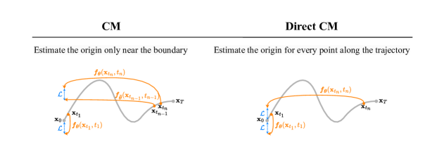
Figure 1: CMs (left) are weakly supervised ODE solvers, only learning to map points along a trajectory that are near the trajectory’s origin back to the origin itself; points that are far from the origin instead enforce a self-consistency property, relying on weak self-supervision to solve the PF ODE. Direct CMs (right) are strongly supervised ODE solvers, instead learning to directly map all points along a trajectory back to the origin.

In Equation 4, $\mathbf{x}_{0}$ and $\mathbf{x}_{t_{n}}$ do not belong to the same ODE trajectory since noise is added to obtain $\mathbf{x}_{t_{n}}$ from $\mathbf{x}_{0}$ via the forward SDE’s transition kernel. Thus, it would not make sense to enforce consistency by minimizing $d(\boldsymbol{f_{\theta}}(\mathbf{x}_{t_{n}},t_{n}),\mathbf{x}_{0})$, and Equation 4 is used instead. While Song et al. [49] theoretically showed that perfectly minimizing Equation 4 with an arbitrarily flexible $\boldsymbol{f_{\theta}}$ results in $\boldsymbol{f_{\theta}}(\mathbf{x}_{t_{n}},t_{n})=\boldsymbol{f_{\texttt{solver}}}(\mathbf{x}_{t_{n}},t_{n},0)$, in practice it has been observed that CMs can be difficult to optimize, with slow convergence or, in some cases, divergence [10, 7]. We attribute this behaviour to what we call “weak supervision” in the CM loss, namely that $\boldsymbol{f_{\theta}}$ is not directly trained to map $\mathbf{x}_{t_{n}}$ to the origin of its ODE trajectory. The constraint that the CM should map any point on the ODE trajectory to the trajectory’s origin is only weakly enforced through the boundary condition parameterization of $\boldsymbol{f_{\theta}}$. Only at time $t_{1}$ does the objective directly encourage mapping points $\mathbf{x}_{t_{1}}$ to the trajectory’s origin. The network $\boldsymbol{f_{\theta}}$ must therefore first learn to map slightly noised data back to the origin before that constraint can be properly enforced for noisier inputs at larger timesteps. We depict this behaviour in Figure 1 (left).

In order to assess the impact of ODE solving on CMs, we put forth a more intuitive and interpretable variation of its loss as

$$\mathcal{L}_{\text{CD}}^{\text{Direct}}:=\mathbb{E}_{\mathbf{x}_{0}\sim p_{0},n\sim\mathcal{U}\llbracket 1,N\rrbracket,\mathbf{x}_{t_{n}}\sim p_{t_{n}\mid 0}(\cdot\mid\mathbf{x}_{0})}\Big{[}\lambda(t_{n})d\Big{(}\boldsymbol{f_{\theta}}(\mathbf{x}_{t_{n}},t_{n}),\boldsymbol{f_{\texttt{solver}}}(\mathbf{x}_{t_{n}},t_{n},0)\Big{)}\Big{]},$$ (5)

where we directly enforce that all points along a trajectory map to its origin, rather than providing only weak supervision as in CMs; see Figure 1 (right). We see this loss as the smallest possible modification to CMs resulting in the direct matching of the model and the solver. Note that unlike standard CMs, Direct CMs do not require enforcing the boundary condition in the parameterization of $\boldsymbol{f_{\theta}}$ to prevent collapse, although it is of course still valid to do so. While this loss requires solving the ODE for $n$ steps at each iteration and is therefore more computationally expensive than Equation 4, we only propose this formulation for comparative purposes rather than suggesting its use in practice.

As we will show, Equation 5 does indeed solve the empirical PF ODE better than Equation 4 but, intriguingly, it translates to worse sample quality. We define the ODE solving error $\mathcal{E}$ as the expected distance between the ODE solver’s solution and the CM’s prediction with the same initial noise, i.e.,

$$\mathcal{E}:=\mathbb{E}_{\mathbf{x}_{T}\sim\widehat{p}_{T}}\Big{[}d\Big{(}\boldsymbol{f_{\theta}}(\mathbf{x}_{T},T),\boldsymbol{f_{\texttt{solver}}}(\mathbf{x}_{T},T,0)\Big{)}\Big{]}.$$ (6)

4 Experiments

Table 1: Results of ODE solving and image quality for single-step generation. CMs perform worse at solving the PF ODE but produce higher quality images.

$\Phi$	Method	ODE	Image
		$\mathcal{E}\downarrow$	FID $\downarrow$	FD-DINO $\downarrow$	CLIP $\uparrow$	Aes $\uparrow$
DDIM	CM	0.29	103.9	816.3	0.21	5.6
	Direct CM	0.25	158.6	1095	0.20	5.1
Euler	CM	0.29	95.3	747.7	0.21	5.5
	Direct CM	0.23	166.0	1148	0.19	5.0
Heun	CM	0.30	120.5	846.1	0.21	5.5
	Direct CM	0.25	162.0	1126	0.19	5.1

Training

For all of our experiments, we aim to compare CMs and Direct CMs using large-scale and state-of-the-art DMs trained on Internet-scale data to better reflect the performance of these models in practical real-world settings. Hence, we select SDXL [30] as the DM to distill, a text-to-image latent diffusion model [36] with a 2.6 B parameter U-Net backbone [37], capable of generating images at a 1024 px resolution. Classifier-free guidance [13] is commonly used to improve sample quality in text-conditional DMs, so we augment $\boldsymbol{s}$ in Equation 3 as $\boldsymbol{s}(\mathbf{x}_{t},t,c,\omega)$, where $c$ is the text prompt and $\omega$ is the guidance scale, following Luo et al. [25]. When distilling a DM, it is common to initialize the student network from the weights of the teacher network so that, in effect, distillation is reduced to a fine-tuning task which requires much less data and resources. We further leverage modern best practices for efficient fine-tuning using low-rank adapters [16, 26]. We use a high-quality subset of the LAION-5B dataset [43] called LAION-Aesthetics-6.5+ for training similar to Luo et al. [25]. To ensure a controlled comparison of CMs and Direct CMs, the only component in the code that we modify is the loss. See Appendix A.1 for a list of training hyperparameters.

Evaluation

We perform quantitative comparisons using metrics that measure ODE solving quality as well as image quality. For ODE solving, we use $\mathcal{E}$ (Equation 6, lower is better) which is only valid for single-step generation. For image metrics, we use Fréchet Distance on Inception (FID [12], lower is better) and DINOv2 (FD-DINO [28, 50], lower is better) latent spaces to assess distributional quality, CLIP score (CLIP [33, 11], higher is better) for prompt-image alignment, and aesthetic score (Aes [35], higher is better) as a proxy to subjective visual appeal. All generated samples use fixed seeds to ensure consistent random noise. The reference dataset for both FID and FD-DINO uses 10k samples generated from the teacher with the same seeds.

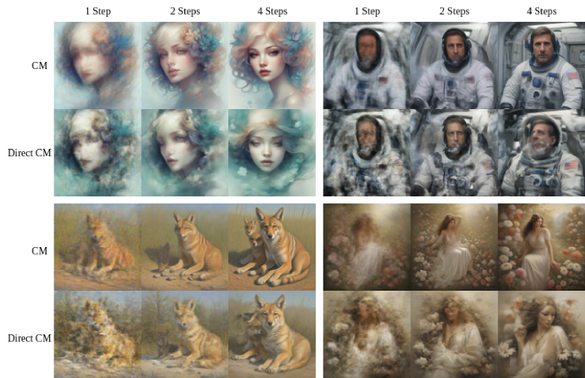
Figure 2: Samples generated by both CMs and Direct CMs. The samples produced by CMs are clearly of higher quality. All corresponding images are generated from the same initial noise.

Quantitative Analysis

We provide a quantitative evaluation of CMs and Direct CMs in Table 1. We show performance for three different choices of numerical ODE solvers $\Phi$, namely DDIM [45] following Luo et al. [25], Euler [8], and Heun [38] following Song et al. [49]. As mentioned earlier, $\mathcal{E}$ is a meaningful metric for ODE-solving fidelity only for single-step generation, so we focus our main quantitative analysis on single-step generation; we provide additional image-based metrics for two- and four-step generation in Appendix A.2 for completeness. Across all image-based metrics in Table 1, we observe that CMs convincingly outperform Direct CMs, meaning that training with Equation 4 results in largely superior image quality than training with Equation 5. However, in terms of their ability to more accurately solve the PF ODE, we find that Direct CMs are consistently better. Ironically, the objective of CMs, as presented by Song et al. [49], is motivated by learning to faithfully solve the PF ODE, so it is highly surprising that more accurate solving can translate to worse image quality.

Our experiments suggest that the pursuit of diffusion model distillation methods to better solve the PF ODE might be a red herring, and that it is not in complete alignment with the goal of generating high-quality samples. Several follow-up works to CMs [46, 7] have further built upon the PF ODE formulation, proposing variations to CMs such as splitting the trajectory into segments [10, 57] or learning to solve the ODE bidirectionally [21] for example. Although they observed better sample quality, we reject the notion that their improvements are strictly entailed by better PF ODE solving. Our results in Table 1 suggest that the high quality of images produced by ODE solving methods (such as CMs and variations) cannot be fully attributed to their ODE solving fidelity; confounding factors should be considered as well.

Moreover, we argue that this observed discrepancy between ODE solving and sample quality might suggest that PF ODE solving on its own may not be the most reliable approach to distill a diffusion model in practice. It is perhaps unsurprising then that several follow-up works improving upon CMs rely on auxiliary losses to supplement ODE solving such as adversarial [18, 3, 51, 19], distribution matching [3, 35], and human feedback learning [54, 35] losses.

Qualitative Comparison

We corroborate our observations with a qualitative comparison of CMs and Direct CMs in Figure 2, and include additional samples in Appendix A.3. We show generated samples from a fixed seed for one, two and four sampling steps using text prompts from the training set. It is clear that CMs produce higher-quality samples than Direct CMs with better high frequency details and fewer artifacts.

Ablations

To ensure that our findings are agnostic to hyperparameter selection in the underlying PF ODE and ODE solver, we sweep over various discretization intervals $N\in\{25,50,100,200\}$ and guidance scales $\omega\in\{1,4,8,11\}$, and provide results for single-step generation in Figure 3 and Figure 4. Regardless of the teacher’s guidance scale and discretization, Direct CMs solve the PF ODE more accurately, yet CMs produce higher quality images.

Figure 3: Effect of the teacher’s number of discretization intervals $N$. In all cases, we observe that Direct CMs are better at solving the PF ODE, but CMs produce higher quality images.

Figure 4: Effect of the teacher’s guidance scale $\omega$. We use $N=50$ here for faster experimentation. In all cases, we observe that Direct CMs are better at solving the PF ODE, but CMs produce higher quality images.

5 Conclusions and Future Work

Although consistency models have achieved success in distilling diffusion models into few-step generators, we find that there exists a gap between their theory and practice. Solving the PF ODE is central to the theoretical motivation of CMs, but we show that we can solve the same PF ODE more accurately using Direct CMs while generating samples of noticeably worse quality. Naturally, we question what additional underlying factors might be contributing to the effectiveness of CMs, and call for additional research from the community to bridge this observed gap between solving the PF ODE and generating high-quality samples. We finish by putting forth some potential explanations: $(i)$ since our experiments are carried out with latent diffusion models, the ODEs are defined on the corresponding latent space, and it could be that the closeness to the solver’s solutions observed in Direct CMs is undone after decoding to pixel space; $(ii)$ if the pre-trained diffusion model failed to closely approximate the true score function (as could be the case when the true score function is unbounded [29, 23, 22]) then $\boldsymbol{f}_{s}\not\approx\boldsymbol{f}_{*}$, meaning that even if a model closely approximates $\boldsymbol{f_{\texttt{solver}}}$ and thus $\boldsymbol{f}_{s}$, it need not be the case that it also properly approximates $\boldsymbol{f}_{*}$; and $(iii)$ although both the CM and Direct CM objectives (Equation 4 and Equation 5, respectively) are meant to mimic the solver $\boldsymbol{f_{\texttt{solver}}}$ at optimality, in practice this optimum is never perfectly achieved, and the CM objective might inadvertently provide a beneficial inductive bias which improves sample quality.

Appendix A Appendix

A.1 Hyperparameters

We provide a list of default hyperparameter values in Table 2. We only train a small number of LoRA blocks [16] following Luo et al. [26], and find that metric and loss curves stabilized around 250 training steps. To enforce the boundary condition in CMs, we follow Song et al. [49] and parameterize $\boldsymbol{f_{\theta}}(\mathbf{x}_{t_{n}},t_{n})=c_{\text{skip}}(t_{n})\mathbf{x}_{t_{n}}+c_{\text{out}}(t_{n})F_{\boldsymbol{\theta}}(\mathbf{x}_{t_{n}},t_{n})$ where $F_{\boldsymbol{\theta}}(\mathbf{x}_{t_{n}},t_{n})$ in our case is the SDXL U-Net backbone with learnable LoRA blocks, and $c_{\text{skip}}(t_{n})$ and $c_{\text{out}}(t_{n})$ are differentiable functions such that $c_{\text{skip}}(0)=1$ and $c_{\text{out}}(0)=0$. We set the values of $c_{\text{skip}}(t_{n})$ and $c_{\text{out}}(t_{n})$ following Luo et al. [25] (see Table 2), and note that this choice is roughly equivalent to a step function where, for $n\geq 1$, $c_{\text{skip}}(t_{n})\approx 0$ and $c_{\text{out}}(t_{n})\approx 1$. As mentioned in the main text, Direct CMs do not require enforcing a boundary condition by construction, but we parameterize them identically to CMs in order to ensure controlled experiments so that we can attribute any differences between them solely to differences in the loss. All experiments were performed on a single 48GB NVIDIA RTX 6000 Ada GPU.

Table 2: Default hyperparameters for both CMs and Direct CMs, unless otherwise specified.

Hyperparameter	Default Setting
Batch size	16
Mixed precision	fp16
Efficient attention [32]	True
Gradient checkpointing	True
Optimizer	8-bit Adam [6]
Adam weight decay	$10^{-2}$
Num. training steps	250
LoRA $r$ [16]	64
LoRA $\alpha$ [16]	64
Learning rate scheduler	Constant
Learning rate warmup steps	0
Learning rate	$10^{-4}$
$\Phi$	DDIM [45]
$N$	100
$\omega$	8
$d(\cdot,\cdot)$	Squared $L_{2}$ distance
$\lambda(t)$	1
$\sigma_{\text{data}}$	0.5 [49]
$\tau$	10
$c_{\text{skip}}(t)$	$\frac{\sigma_{\text{data}}^{2}}{(t\cdot\tau)^{2}+\sigma_{\text{data}}^{2}}$
$c_{\text{out}}(t)$	$\frac{t\cdot\tau}{\sqrt{(t\cdot\tau)^{2}+\sigma_{\text{data}}^{2}}}$

A.2 Additional Quantitative Results

Table 3: Additional image results for two- and four-step generation.

$\Phi$	Method	ODE	Image
		$\mathcal{E}\downarrow$	FID $\downarrow$			FD-DINO $\downarrow$			CLIP $\uparrow$			Aes $\uparrow$
		1-step	1-step	2-step	4-step	1-step	2-step	4-step	1-step	2-step	4-step	1-step	2-step	4-step
DDIM	CM	0.29	103.9	33.4	19.8	816.3	255.4	159.8	0.21	0.27	0.27	5.6	6.4	6.7
	Direct CM	0.25	158.6	55.0	21.2	1095	346.8	155.1	0.20	0.26	0.28	5.1	6.2	6.5
Euler	CM	0.29	95.3	27.4	18.9	747.7	221.3	156.8	0.21	0.27	0.27	5.5	6.5	6.7
	Direct CM	0.23	166.0	55.7	22.5	1148	357.3	152.7	0.19	0.25	0.27	5.0	6.1	6.4
Heun	CM	0.30	120.5	33.5	20.7	846.1	233.4	159.4	0.21	0.27	0.27	5.5	6.5	6.7
	Direct CM	0.25	162.0	54.8	21.0	1126	341.6	150.6	0.19	0.26	0.28	5.1	6.2	6.4

We provide additional quantitative image analysis for two- and four-step generation in Table 3. In almost all cases, these results demonstrate that CMs generate higher quality images than Direct CMs akin to the single-step generation case. Although these results suggest that for four steps Direct CMs slightly outperform CMs in terms of FD-DINO and CLIP score, qualitative comparisons of generated images between both models (see examples in Figure 2 and Figure 5) quickly reveal that images from CMs have noticeably higher quality. We thus attribute the discrepancy either to imperfections in generative model evaluation metrics as observed by Stein et al. [50], or to these metrics not perfectly matching aesthetic quality and being affected by additional confounders (e.g., FD-DINO scores are meant to reflect image diversity in addition to image aesthetics).

A.3 Additional Qualitative Results

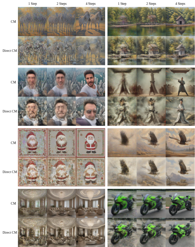
Figure 5: Additional images generated by both CMs and Direct CMs, further highlighting the sample quality difference between the two models. All corresponding images are generated from the same initial noise.

References

- Berthelot et al. [2023] David Berthelot, Arnaud Autef, Jierui Lin, Dian Ang Yap, Shuangfei Zhai, Siyuan Hu, Daniel Zheng, Walter Talbott, and Eric Gu. Tract: Denoising diffusion models with transitive closure time-distillation. arXiv:2303.04248, 2023.
- Blattmann et al. [2023] Andreas Blattmann, Tim Dockhorn, Sumith Kulal, Daniel Mendelevitch, Maciej Kilian, Dominik Lorenz, Yam Levi, Zion English, Vikram Voleti, Adam Letts, Varun Jampani, and Robin Rombach. Stable video diffusion: Scaling latent video diffusion models to large datasets. arXiv:2311.15127, 2023.
- Chadebec et al. [2024] Clement Chadebec, Onur Tasar, Eyal Benaroche, and Benjamin Aubin. Flash diffusion: Accelerating any conditional diffusion model for few steps image generation. arXiv:2406.02347, 2024.
- Chen et al. [2023] Sitan Chen, Sinho Chewi, Jerry Li, Yuanzhi Li, Adil Salim, and Anru Zhang. Sampling is as easy as learning the score: Theory for diffusion models with minimal data assumptions. In The Eleventh International Conference on Learning Representations, 2023.
- Dai et al. [2023] Xiaoliang Dai, Ji Hou, Chih-Yao Ma, Sam Tsai, Jialiang Wang, Rui Wang, Peizhao Zhang, Simon Vandenhende, Xiaofang Wang, Abhimanyu Dubey, Matthew Yu, Abhishek Kadian, Filip Radenovic, Dhruv Mahajan, Kunpeng Li, Yue Zhao, Vladan Petrovic, Mitesh Kumar Singh, Simran Motwani, Yi Wen, Yiwen Song, Roshan Sumbaly, Vignesh Ramanathan, Zijian He, Peter Vajda, and Devi Parikh. Emu: Enhancing image generation models using photogenic needles in a haystack. arXiv:2309.15807, 2023.
- Dettmers et al. [2022] Tim Dettmers, Mike Lewis, Sam Shleifer, and Luke Zettlemoyer. 8-bit optimizers via block-wise quantization. In International Conference on Learning Representations, 2022.
- Geng et al. [2024] Zhengyang Geng, Ashwini Pokle, William Luo, Justin Lin, and J Zico Kolter. Consistency models made easy. arXiv:2406.14548, 2024.
- Griffiths and Higham [2010] David F. Griffiths and Desmond J. Higham. Numerical Methods for Ordinary Differential Equations. Springer, 2010.
- Gu et al. [2023] Jiatao Gu, Shuangfei Zhai, Yizhe Zhang, Lingjie Liu, and Joshua M Susskind. Boot: Data-free distillation of denoising diffusion models with bootstrapping. In ICML 2023 Workshop on Structured Probabilistic Inference & Generative Modeling, 2023.
- Heek et al. [2024] Jonathan Heek, Emiel Hoogeboom, and Tim Salimans. Multistep consistency models. arXiv:2403.06807, 2024.
- Hessel et al. [2021] Jack Hessel, Ari Holtzman, Maxwell Forbes, Ronan Le Bras, and Yejin Choi. CLIPScore: A Reference-free Evaluation Metric for Image Captioning. In Proceedings of the 2021 Conference on Empirical Methods in Natural Language Processing, 2021. doi: 10.18653/v1/2021.emnlp-main.595.
- Heusel et al. [2017] Martin Heusel, Hubert Ramsauer, Thomas Unterthiner, Bernhard Nessler, and Sepp Hochreiter. GANs Trained by a Two Time-Scale Update Rule Converge to a Local Nash Equilibrium. In Advances in Neural Information Processing Systems, volume 30, 2017.
- Ho and Salimans [2022] Jonathan Ho and Tim Salimans. Classifier-free diffusion guidance. arXiv:2207.12598, 2022.
- Ho et al. [2020] Jonathan Ho, Ajay Jain, and Pieter Abbeel. Denoising diffusion probabilistic models. In Advances in Neural Information Processing Systems, volume 33, 2020.
- Ho et al. [2022] Jonathan Ho, Tim Salimans, Alexey Gritsenko, William Chan, Mohammad Norouzi, and David J Fleet. Video diffusion models. In Advances in Neural Information Processing Systems, volume 35, 2022.
- Hu et al. [2022] Edward J Hu, yelong shen, Phillip Wallis, Zeyuan Allen-Zhu, Yuanzhi Li, Shean Wang, Lu Wang, and Weizhu Chen. LoRA: Low-Rank Adaptation of Large Language Models. In International Conference on Learning Representations, 2022.
- Huang et al. [2023] Rongjie Huang, Jiawei Huang, Dongchao Yang, Yi Ren, Luping Liu, Mingze Li, Zhenhui Ye, Jinglin Liu, Xiang Yin, and Zhou Zhao. Make-an-audio: Text-to-audio generation with prompt-enhanced diffusion models. In Proceedings of the 40th International Conference on Machine Learning, 2023.
- Kim et al. [2024a] Dongjun Kim, Chieh-Hsin Lai, Wei-Hsiang Liao, Naoki Murata, Yuhta Takida, Toshimitsu Uesaka, Yutong He, Yuki Mitsufuji, and Stefano Ermon. Consistency trajectory models: Learning probability flow ODE trajectory of diffusion. In The Twelfth International Conference on Learning Representations, 2024a.
- Kim et al. [2024b] Dongjun Kim, Chieh-Hsin Lai, Wei-Hsiang Liao, Yuhta Takida, Naoki Murata, Toshimitsu Uesaka, Yuki Mitsufuji, and Stefano Ermon. PaGoDA: Progressive Growing of a One-Step Generator from a Low-Resolution Diffusion Teacher. arXiv:2405.14822, 2024b.
- Kong et al. [2021] Zhifeng Kong, Wei Ping, Jiaji Huang, Kexin Zhao, and Bryan Catanzaro. Diffwave: A versatile diffusion model for audio synthesis. In International Conference on Learning Representations, 2021.
- Li and He [2024] Liangchen Li and Jiajun He. Bidirectional consistency models. arXiv:2403.18035, 2024.
- Loaiza-Ganem et al. [2024] Gabriel Loaiza-Ganem, Brendan Leigh Ross, Rasa Hosseinzadeh, Anthony L Caterini, and Jesse C Cresswell. Deep generative models through the lens of the manifold hypothesis: A survey and new connections. Transactions on Machine Learning Research, 2024.
- Lu et al. [2023] Yubin Lu, Zhongjian Wang, and Guillaume Bal. Mathematical analysis of singularities in the diffusion model under the submanifold assumption. arXiv:2301.07882, 2023.
- Luhman and Luhman [2021] Eric Luhman and Troy Luhman. Knowledge distillation in iterative generative models for improved sampling speed. arXiv:2101.02388, 2021.
- Luo et al. [2023a] Simian Luo, Yiqin Tan, Longbo Huang, Jian Li, and Hang Zhao. Latent consistency models: Synthesizing high-resolution images with few-step inference. arXiv:2310.04378, 2023a.
- Luo et al. [2023b] Simian Luo, Yiqin Tan, Suraj Patil, Daniel Gu, Patrick von Platen, Apolinário Passos, Longbo Huang, Jian Li, and Hang Zhao. LCM-LoRA: A universal stable-diffusion acceleration module. arXiv:2311.05556, 2023b.
- Meng et al. [2023] Chenlin Meng, Robin Rombach, Ruiqi Gao, Diederik Kingma, Stefano Ermon, Jonathan Ho, and Tim Salimans. On distillation of guided diffusion models. In Proceedings of the IEEE/CVF Conference on Computer Vision and Pattern Recognition, pages 14297–14306, 2023.
- Oquab et al. [2024] Maxime Oquab, Timothée Darcet, Théo Moutakanni, Huy V. Vo, Marc Szafraniec, Vasil Khalidov, Pierre Fernandez, Daniel HAZIZA, Francisco Massa, Alaaeldin El-Nouby, Mido Assran, Nicolas Ballas, Wojciech Galuba, Russell Howes, Po-Yao Huang, Shang-Wen Li, Ishan Misra, Michael Rabbat, Vasu Sharma, Gabriel Synnaeve, Hu Xu, Herve Jegou, Julien Mairal, Patrick Labatut, Armand Joulin, and Piotr Bojanowski. DINOv2: Learning robust visual features without supervision. Transactions on Machine Learning Research, 2024. ISSN 2835-8856.
- Pidstrigach [2022] Jakiw Pidstrigach. Score-based generative models detect manifolds. In Advances in Neural Information Processing Systems, volume 35, 2022.
- Podell et al. [2024] Dustin Podell, Zion English, Kyle Lacey, Andreas Blattmann, Tim Dockhorn, Jonas Müller, Joe Penna, and Robin Rombach. SDXL: Improving Latent Diffusion Models for High-Resolution Image Synthesis. In The Twelfth International Conference on Learning Representations, 2024.
- Poole et al. [2023] Ben Poole, Ajay Jain, Jonathan T. Barron, and Ben Mildenhall. Dreamfusion: Text-to-3d using 2d diffusion. In The Eleventh International Conference on Learning Representations, 2023.
- Rabe and Staats [2021] Markus N Rabe and Charles Staats. Self-attention Does Not Need Memory. arXiv:2112.05682, 2021.
- Radford et al. [2021] Alec Radford, Jong Wook Kim, Chris Hallacy, Aditya Ramesh, Gabriel Goh, Sandhini Agarwal, Girish Sastry, Amanda Askell, Pamela Mishkin, Jack Clark, Gretchen Krueger, and Ilya Sutskever. Learning transferable visual models from natural language supervision. In Proceedings of the 38th International Conference on Machine Learning, volume 139, 2021.
- Ramesh et al. [2022] Aditya Ramesh, Prafulla Dhariwal, Alex Nichol, Casey Chu, and Mark Chen. Hierarchical text-conditional image generation with clip latents. arXiv:2204.06125, 2022.
- Ren et al. [2024] Yuxi Ren, Xin Xia, Yanzuo Lu, Jiacheng Zhang, Jie Wu, Pan Xie, Xing Wang, and Xuefeng Xiao. Hyper-SD: Trajectory Segmented Consistency Model for Efficient Image Synthesis. arXiv:2404.13686, 2024.
- Rombach et al. [2022] Robin Rombach, Andreas Blattmann, Dominik Lorenz, Patrick Esser, and Björn Ommer. High-resolution image synthesis with latent diffusion models. In Proceedings of the IEEE/CVF Conference on Computer Vision and Pattern Recognition, 2022.
- Ronneberger et al. [2015] Olaf Ronneberger, Philipp Fischer, and Thomas Brox. U-net: Convolutional networks for biomedical image segmentation. In Medical image computing and computer-assisted intervention–MICCAI 2015: 18th international conference, Munich, Germany, October 5-9, 2015, proceedings, part III 18, pages 234–241. Springer, 2015.
- Ronveaux and Arscott [1995] André Ronveaux and F. M. Arscott. Heun’s Differential Equations. Oxford University Press, 1995.
- Ruan et al. [2023] Ludan Ruan, Yiyang Ma, Huan Yang, Huiguo He, Bei Liu, Jianlong Fu, Nicholas Jing Yuan, Qin Jin, and Baining Guo. MM-Diffusion: Learning Multi-Modal Diffusion Models for Joint Audio and Video Generation. In Proceedings of the IEEE/CVF Conference on Computer Vision and Pattern Recognition, 2023.
- Saharia et al. [2022] Chitwan Saharia, William Chan, Saurabh Saxena, Lala Li, Jay Whang, Emily L Denton, Kamyar Ghasemipour, Raphael Gontijo Lopes, Burcu Karagol Ayan, Tim Salimans, Jonathan Ho, David J Fleet, and Mohammad Norouzi. Photorealistic text-to-image diffusion models with deep language understanding. In Advances in Neural Information Processing Systems, volume 35, 2022.
- Salimans and Ho [2022] Tim Salimans and Jonathan Ho. Progressive distillation for fast sampling of diffusion models. In International Conference on Learning Representations, 2022.
- Sauer et al. [2023] Axel Sauer, Dominik Lorenz, Andreas Blattmann, and Robin Rombach. Adversarial diffusion distillation. arXiv:2311.17042, 2023.
- Schuhmann et al. [2022] Christoph Schuhmann, Romain Beaumont, Richard Vencu, Cade Gordon, Ross Wightman, Mehdi Cherti, Theo Coombes, Aarush Katta, Clayton Mullis, Mitchell Wortsman, Patrick Schramowski, Srivatsa Kundurthy, Katherine Crowson, Ludwig Schmidt, Robert Kaczmarczyk, and Jenia Jitsev. LAION-5B: An open large-scale dataset for training next generation image-text models. In Advances in Neural Information Processing Systems, volume 35, 2022.
- Sohl-Dickstein et al. [2015] Jascha Sohl-Dickstein, Eric Weiss, Niru Maheswaranathan, and Surya Ganguli. Deep unsupervised learning using nonequilibrium thermodynamics. In Proceedings of the 32nd International Conference on Machine Learning, volume 37, 2015.
- Song et al. [2021a] Jiaming Song, Chenlin Meng, and Stefano Ermon. Denoising diffusion implicit models. In International Conference on Learning Representations, 2021a.
- Song and Dhariwal [2024] Yang Song and Prafulla Dhariwal. Improved techniques for training consistency models. In The Twelfth International Conference on Learning Representations, 2024.
- Song and Ermon [2020] Yang Song and Stefano Ermon. Improved techniques for training score-based generative models. In Advances in Neural Information Processing Systems, volume 33, 2020.
- Song et al. [2021b] Yang Song, Jascha Sohl-Dickstein, Diederik P Kingma, Abhishek Kumar, Stefano Ermon, and Ben Poole. Score-based generative modeling through stochastic differential equations. In International Conference on Learning Representations, 2021b.
- Song et al. [2023] Yang Song, Prafulla Dhariwal, Mark Chen, and Ilya Sutskever. Consistency models. In Proceedings of the 40th International Conference on Machine Learning, volume 202, 2023.
- Stein et al. [2023] George Stein, Jesse C Cresswell, Rasa Hosseinzadeh, Yi Sui, Brendan Ross, Valentin Villecroze, Zhaoyan Liu, Anthony L Caterini, J Eric T Taylor, and Gabriel Loaiza-Ganem. Exposing flaws of generative model evaluation metrics and their unfair treatment of diffusion models. In Advances in Neural Information Processing Systems, volume 36, 2023.
- Wang et al. [2024] Fu-Yun Wang, Zhaoyang Huang, Alexander William Bergman, Dazhong Shen, Peng Gao, Michael Lingelbach, Keqiang Sun, Weikang Bian, Guanglu Song, Yu Liu, Hongsheng Li, and Xiaogang Wang. Phased consistency model. arXiv:2405.18407, 2024.
- Wang et al. [2023] Xiang Wang, Hangjie Yuan, Shiwei Zhang, Dayou Chen, Jiuniu Wang, Yingya Zhang, Yujun Shen, Deli Zhao, and Jingren Zhou. VideoComposer: Compositional Video Synthesis with Motion Controllability. In Advances in Neural Information Processing Systems, volume 36, 2023.
- Wu et al. [2023] Jay Zhangjie Wu, Yixiao Ge, Xintao Wang, Stan Weixian Lei, Yuchao Gu, Yufei Shi, Wynne Hsu, Ying Shan, Xiaohu Qie, and Mike Zheng Shou. Tune-a-video: One-shot tuning of image diffusion models for text-to-video generation. In Proceedings of the IEEE/CVF International Conference on Computer Vision, 2023.
- Xie et al. [2024] Qingsong Xie, Zhenyi Liao, Chen chen, Zhijie Deng, Shixiang Tang, and Haonan Lu. MLCM: Multistep Consistency Distillation of Latent Diffusion Model. arXiv:2406.05768, 2024.
- Yin et al. [2024] Tianwei Yin, Michaël Gharbi, Richard Zhang, Eli Shechtman, Frédo Durand, William T. Freeman, and Taesung Park. One-step diffusion with distribution matching distillation. In Proceedings of the IEEE/CVF Conference on Computer Vision and Pattern Recognition, 2024.
- Zheng et al. [2023] Hongkai Zheng, Weili Nie, Arash Vahdat, Kamyar Azizzadenesheli, and Anima Anandkumar. Fast sampling of diffusion models via operator learning. In Proceedings of the 40th International Conference on Machine Learning, volume 202, 2023.
- Zheng et al. [2024] Jianbin Zheng, Minghui Hu, Zhongyi Fan, Chaoyue Wang, Changxing Ding, Dacheng Tao, and Tat-Jen Cham. Trajectory consistency distillation. arXiv:2402.19159, 2024.