Anonymous Distributed Localisation via
Spatial Population Protocols
Abstract
In the distributed localization problem (DLP), anonymous robots (agents) begin at arbitrary positions , where is a Euclidean space. Initially, each agent operates within its own coordinate system in , which may be inconsistent with those of other agents. The primary goal in DLP is for agents to reach a consensus on a unified coordinate system that accurately reflects the relative positions of all points, , in . Extensive research on DLP has primarily focused on the feasibility and complexity of achieving consensus when agents have limited access to inter-agent distances, often due to missing or imprecise data. In this paper, however, we examine a minimalist, computationally efficient model of distributed computing in which agents have access to all pairwise distances, if needed. Specifically, we introduce a novel variant of population protocols, referred to as the spatial population protocols model. In this variant each agent can memorise one or a fixed number of coordinates, and when agents and interact, they can not only exchange their current knowledge but also either determine the distance between them in (distance query model) or obtain the vector spanning points and (vector query model).
We examine three DLP scenarios, proposing and analysing several types of distributed localisation protocols, including:
-
1.
Self-stabilising localisation protocol with distance queries We propose and analyse self-stabilising localisation protocol based on pairwise distance adjustment. We also discuss several hard instances in this scenario, and suggest possible improvements for the considered protocol,
-
2.
Leader-based localisation protocol with distance queries We propose and analyse several leader-based protocols which stabilise in parallel time. These protocols rely on efficient solution to multi-contact epidemic, an extension of one-way epidemic in population protocols, and
-
3.
Self-stabilising localisation protocol with vector queries We propose and analyse superfast self-stabilising DLP protocol which stabilises in parallel time.
We conclude with a discussion on future research directions for distributed localization in spatial population protocols, including scenarios that account for higher dimensions, limited precision and susceptibility to errors.
1 Introduction
Location services are crucial for modern computing paradigms, such as pervasive computing and sensor networks. While manual configuration and GPS can determine node locations, these methods are impractical in large-scale or obstructed environments. Recent approaches use network localisation, where beacon nodes with known positions enable other nodes to estimate their locations via distance measurements. Key challenges remain, including determining conditions for unique localisability, computational complexity, and deployment considerations. In the distributed localisation problem (DLP), anonymous robots (agents) begin at arbitrary positions , where is a Euclidean space. Initially, each agent operates within its own coordinate system in , which may be inconsistent with those of other agents. The primary goal in DLP is for agents to reach a consensus on a unified coordinate system that accurately reflects the relative positions of all points, , in .
A network of agents’ unique localisability is determined by specific combinatorial properties of its graph and the number of anchors (agents aware of their real location). For example, graph rigidity theory [13, 17, 18] provides a necessary and sufficient condition for unique localisability [13]. Specifically, a network of agents located in the plane is uniquely localisable if and only if it has at least three anchors and the network graph is globally rigid. However, unless a network is dense and regular, global rigidity is unlikely. Even without global rigidity, large portions of a network may still be globally rigid, though positions of remaining nodes will remain indeterminate due to multiple feasible solutions. The decision version of this problem, often referred to as the graph embedding or graph realisation problem, requires determining whether a weighted graph can be embedded in the plane so that distances between adjacent vertices match the edge weights, a problem known to be strongly NP-hard [26]. Furthermore, this complexity holds even when the graph is globally rigid [13]. In sensor networks, where nodes measure distances only within a communication range , the network is best represented as a unit disk graph. Here, two nodes are adjacent if and only if their distance is . The corresponding decision problem, known as unit disk graph reconstruction, requires determining whether a graph can be embedded in the plane such that distances between adjacent nodes match edge weights, while distances between non-adjacent nodes exceed . This problem is also NP-hard [6], indicating that no efficient algorithm can solve localisation in the worst case unless . Furthermore, even for instances with unique reconstructions, no efficient randomised algorithm exists to solve this problem unless [6].
Distributed localisation is also crucial in robotic systems, enabling robots to autonomously determine their spatial position within an environment – a fundamental requirement for applications such as navigation, mapping, and multi-robot coordination [30]. Accurate localisation allows robots to interact more effectively with their surroundings and with each other, facilitating tasks from autonomous driving to warehouse automation and search-and-rescue operations [24, 22]. Localisation approaches generally fall into two broad categories: centralised and distributed systems [31]. Centralised localisation systems, where a central server or leader node computes the locations of all robots, can offer high accuracy but may struggle with scalability and robustness, especially in dynamic or communication-limited environment [21]. In contrast, distributed localisation systems allow each robot to perform localisation computations independently or in collaboration with neighbouring robots, enhancing adaptability and resilience, although this may come at the cost of increased complexity [20, 19]. Within distributed systems, leader-based localisation mechanisms involve one or more designated robots that serve as reference points or coordinators for localisation [14], which can streamline computations but may create single points of failure. Leaderless localisation, where all robots contribute equally to position estimation without relying on specific leader nodes, is advantageous in decentralised applications where flexibility and fault tolerance are paramount [19, 27]. Both methods have been explored using probabilistic [29], geometric [23], and graph-based models [19], with leaderless approaches gaining traction due to their robustness in large-scale and dynamically changing settings. Various methods leverage tools such as Kalman filters [25], particle filters [21], and graph rigidity theory [28] to enhance localisation accuracy and efficiency in complex environments.
1.1 Spatial population protocols
In this paper, we explore a minimalist, computationally efficient model of distributed computing, where agents have probabilistic access to pairwise distances. Our focus is on achieving anonymity while maintaining high time efficiency and minimal use of network resources, including limited local storage (agent state space) and communication. To meet these goals, we introduce a new variant of population protocols, referred to as the spatial population protocols model, specified later in this section.
The population protocol model originates from the seminal work by Angluin et al. [4]. This model provides tools for the formal analysis of pairwise interactions between indistinguishable entities known as agents, which have limited storage, communication, and computational capabilities. When two agents interact, their states change according to a predefined transition function, a core component of the population protocol. It is typically assumed that the agents’ state space is fixed and that the population size is unknown to the agents and is not hard-coded into the transition function. In self-stabilising protocols, the initial configuration of agents’ states is arbitrary. By contrast, non-self-stabilising protocols start with a predefined configuration encoding the input of the given problem. A protocol concludes when it stabilises in a final configuration of states representing the solution. In the probabilistic variant of population protocols, which is also used here, the random scheduler selects an ordered pair of agents at each step—designated as the initiator and the responder—uniformly at random from the entire population. The asymmetry in this pair introduces a valuable source of random bits, which is utilised by population protocols. In this probabilistic setting, besides efficient state utilisation, time complexity is also a primary concern. It is often measured by the number of interactions, , required for the protocol to stabilise in a final configuration. More recently, the focus has shifted to parallel stabilisation time (or simply time), defined as , where is the population size. This measure captures the parallelism of independent, simultaneous interactions, which is leveraged in efficient population protocols that stabilise in time . All protocols presented in sections 3 and 4 are stable (always correct) and guarantee stabilisation time with high probability (whp), defined as for a constant .
Leader election is a fundamental problem in distributed computing, essential for symmetry breaking, synchronisation, and coordination mechanisms. In population protocols, the presence of a leader enables a more efficient computational setup [5], as further utilised in Section 3. However, achieving leader election in this model poses significant challenges. Foundational results [10, 11] demonstrate that it cannot be solved in sublinear time if agents are restricted to a fixed number of states [12]. Further, Alistarh and Gelashvili [3] introduced a protocol stabilising in time with states. Later, Alistarh et al. [1] identified trade-offs between state use and stabilisation time, distinguishing slowly ( states) and rapidly stabilising ( states) protocols. Subsequent work achieved time whp and in expectation with states [9], later reduced to states using synthetic coins [2, 8]. Recent research by Gąsieniec and Stachowiak reduced state usage to while retaining time whp [15]. The expected time of leader election was further optimised to by Gąsieniec et al. in [16] and to the optimal time by Berenbrink et al. in [7].
Spatial embedding and geometric queries
While population protocols provide an elegant and resilient framework for randomised distributed computation, they lack spatial embedding. To address this limitation, we introduce a new spatial variant of population protocols that extends the transition function to include basic geometric queries. In particular, in this model each agent can memorise one or a fixed number of coordinates, and during an interaction of two agents and , in addition to exchange of their current knowledge, the agents can determine:
-
(1) the distance separating them in , in distance query model, and
-
(2) vector spanning points and , in vector query model.
Our contribution
Using the example of the distributed localisation problem, we show that the adopted model provides a natural framework for developing efficient randomised solutions to distributed problems with geometric embeddings, including those in anonymous and self-stabilising settings. We examine three DLP scenarios, proposing and analysing different types of distributed localisation protocols, including:
-
1.
Self-stabilising localisation protocol with distance queries We propose and analyse self-stabilising protocol based on pairwise distance adjustment. We also discuss some hard instances in this scenario, and suggest possible improvements for the considered protocol, see Section 2.
-
2.
Leader-based localisation protocol with distance queries We propose and analyse several leader-based protocols which stabilise in sublinear parallel time. These protocols rely on a novel concept of multi-contact epidemic, an natural extension of one-way epidemic, see Section 3.
-
3.
Self-stabilising localisation protocol with vector queries We propose and analyse a super fast self-stabilising protocol which stabilises in parallel time in this scenario, see Section 4.
We conclude with a discussion on future research directions for distributed localisation in spatial population protocols, including scenarios that account for limited precision and susceptibility to errors.
2 Leaderless localisation in distance query model
In this section, we adopt the distance query model, assuming that is a linear space where agents are arbitrarily positioned at (unknown to the agents) points , respectively. We use notation to denote the distance between agents and where Additionally, each agent possesses a hypothetical coordinate referred to as its label . In this variant of population protocols, during an interaction of with , the initiator learns about distance and label . Let inconsistency . In localisation protocols presented in this section, the labels of agents are gradually adjusted to minimise the maximum inconsistency defined as
If, eventually, , we say that the computed labels are stable. If a localisation protocol achieves for a preset constant , we say that the computed labels are -stable.
Below, we propose and experimentally analyse two localisation protocols. The first, see Section 2.1, a basic Distance-Adjustment protocol, achieves -stabilisation of labels in (parallel) time. In Section 2.2 we examine an enhanced version, the Distance-adjustment-with-doubt protocol, which supports slower but more reliable stabilisation by increasing the confidence of participating agents in their labels.
2.1 Distance-adjustment protocol
We start with presentation of a crude Distance-adjustment protocol in which after initiator contacts when two possible actions are taken. If the initiator updates its label to reduce inconsistency by a predefined adjustment factor and if updates to increase the inconsistency by the same factor where is one of the parameters of the solution.
This label updating principle is utilised in Algorithm 1.
Note, that while an interaction reduces inconsistency between agents and , such local amendment may increase inconsistencies in other pairs of agents involving and in turn making the new labelling further away from the final -stabilisation. While this phenomenon is indeed the source of several complications in the worst case distribution of agents’ positions in , our experiments indicate that Algorithm 1 computes -stable labels effectively in time , when agent’s positions are random.
Example (Hard instance)
One of the instances for which Algorithm 1 struggles to stabilise refers to the initial configuration in which agents are placed in positions:
and the relevant initial labels are:
Intuitively, almost all agents have mutually consistent labels apart from . This agent is positioned at while its label indicates position which is on the ’wrong’ side of the whole group. One can observe, that in such configuration a large fraction of the agents repel while another large fraction attracts it. In consequence, these two strong (attracting and repelling) forces prevent the system from proper ordering of agents and in turn from stabilisation for very long time.
Discussion
Figure 1 shows a typical drop in value of maximum inconsistency during execution of Algorithm 1. In our experiment, at the beginning of each run the agents are uniformly distributed along the line integer assuming fixed distances (equal to ) between subsequent pairs of agents’ positions. The labels are initialised in a random manner and uniformly distributed within an interval times longer than the interval containing the actual agents’ positions. One can observe that during the first phase, the value of drops rapidly until the all labels concentrate in the interval of a similar length to the interval of agents’ positions. Subsequently, during the second phase, the labels gradually become more and more consistent, achieving -stabilisation in time
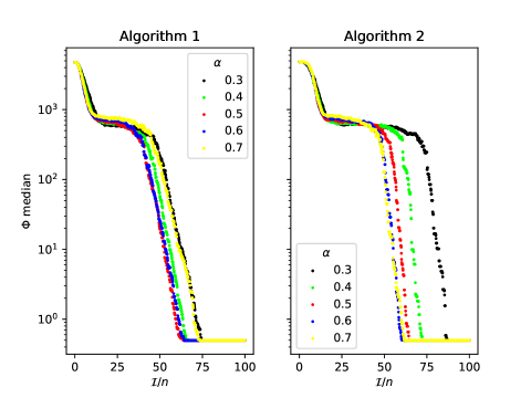
In the next section, we propose an enhancement to this algorithm that performs better on challenging instances, including the one discussed in the example above. However, the increased robustness of the enhanced algorithm comes at the cost of slower and less concentrated time performance, see Figure 1.
2.2 Distance adjustment with doubt protocol
We introduce a new indicator specifying how confident agent is. In particular, when the value of is close to is very confident, and when this value is close to is unconfident (in self-doubt). Intuitively, agents that are confident about their labels experience weaker fluctuations in their doubt. The indicator is computed as a weighted average value of its previous inconsistencies normalised to the interval , we omit the detail here. Intuitively, an agent with a low confidence is likely to be in a local minimum, so it is beneficial to update its label. To capitalise on this observation, in addition to the confidence indicator, we introduce a jumping mechanism that allows an agent with low confidence to update its label more aggressively, with the help of two recently met agents that have very high confidence. This approach is utilised in Algorithm 2, where each agent maintains a list describing the details of recently contacted agents (including their labels, separation distance, and doubt levels). In particular, if the difference between and the second doubt () in the list of recently met agents surpasses the assumed jump threshold agent updates its label to the one determined by the distances to and labels of the two most confident recently met agents. In our experimental setup, data from up to 8 of the most recent interactions were utilised.
We observe, see Figure 2, that the running time of the second phase when agents establish their order on the line, fluctuates significantly and can be long. Conversely, the duration of the final phase, in which the sequence becomes effectively established, is relatively brief. We suppose that due to the latter property the presented approach can be applied to agents that move and whose mutual position is in principle known but requires correction. However, this requires further research.
After this experimental warm-up, we are ready to present and analyse two types of localisation protocols that compute stable labels in time In Section 3, we show that the utilisation of a leader (as an anchor for the computed system of coordinates) enables silent stabilisation through -contact epidemic processes. In Section 4, we demonstrate the power of the model with vector queries, presenting a silent, self-stabilising labelling protocol that stabilises in optimal time in a dimensional space where is a constant.
3 Leader-based localisation in distance query model
In this section, we discuss two localisation protocols with predefined input stabilising in time, i.e., after this time labels of all agents become stable. These protocols are non-self-stabilising. We assume that one of the agents starts as the leader of the population. If the identity of the leader is not known, the localisation protocol can be preceded by one of the leader election protocols discussed in the introduction. The agents’ positions are distributed in a -dimensional Euclidean space , where is a fixed integer. It is assumed that any agents’ positions span the entire space. For example, in two-dimensional space, this assumption guarantees that no three points are collinear. Although our algorithms can be adapted to handle an arbitrary distribution of agents’ positions, the time guarantees of such adaptations would be weaker. The state of an agent can accommodate a fixed number of agent positions and distances.
We adopt a symmetric model of communication, which means that when agents and interact, they both gain access to each other’s states as well as the distance . The transitions assigned to the leader are distinct from those of the other agents, and the leader also serves as the initiator of the entire process. Initially, the state of each agent stores a label (representing a hypothetical position in ) and its color . We assume that at the beginning, the leader is coloured green, and each non-leader’s colour is set to blue. Finally, the leader’s label (position in ) is set at the origin of the coordinate system, i.e., this label is used as the anchor in the localisation process.
3.1 Localisation via multi-contact epidemic
The localisation protocol presented in this section consists of two parts. In the first part of the protocol the labels of agents (including the leader) become stable (positions of these agents become fixed) and these agents become green. The counter initially set to of agents with stable (green) labels is maintained by the leader. In the second part the labels of all remaining (blue) agents become stable. And this is done by contacting with different green agents. And once the agent is positioned, it becomes green. We refer to this (multilateration) process as -contact epidemic, see page 3.1.
Positioning of each of the first agents has to be approved by the leader. More precisely, after an aspiring to be green agent interaction with all green agents is concluded, to become green must meet the leader to get approved. And when this happens, the leader updates the counter of greenagents, and the new green agent is ready to calculate its projection onto the subspace spanned by its green predecessors and the leader, as well as its Euclidean distance from this subspace. Namely, the first coordinates of ’s label are determined by this projection, and the -th coordinate (in newly formed dimension) is equal to its distance from the aforementioned subspace. When positioning the remaining agents, we use the fact that interactions with green agents allow for the unambiguous determination of an agent’s position.
Theorem 1.
Algorithm 3 stabilises labels of all agents in dimensions in time .
Proof.
As mentioned earlier Algorithm 3 operates in two parts. In the the first part, the protocol stabilises the labels of the leader and extra agents, creating an initial set of green agents in time whp (Lemma 2). The second part stabilises labels of all remaining agents via -contact epidemic in time (Theorem 2). ∎
First we formulate a lemma
Lemma 1.
Consider of independent random variables with the expected value for large enough. For any constant , holds whp.
Proof.
The following equality holds
By Chernoff inequalities we get for any parameter
and
Thus . ∎
Now we formulate a lemma determining the time needed to position -th agent during the process of positioning the first green agents.
Lemma 2.
Algorithm 3 (first part), the -th green agent is positioned in time whp.
Proof.
Consider successive periods of length and an additional period of length . We show that after all these periods, whp a new green agent is positioned.
We now prove by induction that after the first periods there are at least agents that had at least interactions with green agents for , where and for ,
We start with the inductive step. Assume that after initial periods there are at least agents with at least contacts, i.e., interactions with at least green agents. Let be a random variable that equals 1 if, at time , an agent with contacts has a new contact with its -th green agent, and 0 otherwise. If in time less than agents had contacts then
After the -th period of length the expected value of is at least
By Lemma 1 this number is at least whp. Thus also the number of agents that had interactions with at least green agents is at least whp.
Furthermore, after periods there are at least agents that experienced contacts. Consider an extra period of length . Let be a random variable that equals 1 if, at time , an agent with contacts has a contact with the leader, and 0 otherwise. If in time none of these agents had interaction with the leader yet, we get
After an extra period of length the expected value of is at least
And by Lemma 1 this number is at least whp. ∎
Multi-contact epidemic
We introduce and analyze the process of -contact epidemic (a multi-contact epidemic with a fixed parameter ), a natural generalization of epidemic dynamics in population protocols. In this process, the population initially contains at least green agents, while the remaining agents are blue. A blue agent turns green after interacting with distinct green agents. We demonstrate that the time complexity of this process is , for any fixed integer .
We begin with two key lemmas to establish this result.
Lemma 3.
The time needed to transition from a configuration with green agents to a configuration with green agents for is
with high probability (whp), for some constant .
Proof.
Assume that the number of green agents is exactly . Consider successive periods of length and an additional period of length . We show that after all these periods, we obtain at least new green agents whp.
We prove by induction that after the first periods there are at least agents that had at least contacts (interactions with green agents) for , where and for ,
Now we prove the inductive step. Assume that after initial periods there are at least agents with least contacts. Let be a random variable that equals 1 if, at time , an agent with contacts experiences a new contact (with its -th green agent), and 0 otherwise. If in time less than agents had contacts
After the -th period of length the expected value of is at least
By Lemma 1 this number is at least whp. Thus also the number of agents that had at least contacts is at least whp.
After periods of length there are at least agents that had at least contacts. Now let us add an additional period of length . We show that after this period we will have at least new green agents whp. Let be a random variable that equals 1 if, at time , an agent with contacts experiences a new contact (with its -th green agent), and 0 otherwise. Note that each time , a new green agent is produced. As long as less than agents became green,
After one extra period of length the expected value is at least . By Lemma 1 this number is at least whp. Thus also the number of newly generated green agents is at least whp. ∎
Lemma 4.
Starting with at least green agents guarantees recolouring all agents to green in time .
Proof.
If there are altogether green agents, then for any blue agent one can define a random variable equal 1 if in time this agent interacts with a new green agent, and 0 otherwise. The probability that a blue agent does not become green is . In time the value . By Lemma 1 whp, i.e., each agent becomes green whp. ∎
Theorem 2.
The stabilisation time of -contact epidemic is whp.
3.2 Faster positioning algorithm
In this section we show how we can make Algorithm 3 working faster on the line, i.e., in a linear space While we focus on one dimension, our observations can be utilised also in higher dimensions. In what follows, we formulate Algorithm 4 which positions agents not only by using 2-contact epidemic but also utilising interactions between agents with a single successful contact coloured later greenish. In the new algorithm we take advantage of the fact that there are only two types of interactions between greenish agents not leading to positioning of both of them. The first type refers to interactions between agents that became greenish via contacting the same green agent. In the second, each of the two interacting greenish agents is at the same distance and on the same side of their unique green contact. We show that these types of interactions do not contribute significantly to the total time of the solution.
Lemma 5.
The time needed to increase the number of green agents from to for is whp.
Proof.
First we consider an initial period of length . The average number of greenish agents produced by green agents in time is . By Lemma 1 this number is at least whp. For any given green agent , one can define a subset of greenish agents originating from contact with agents other than . The cardinality of is on average at least By Lemma 1 this number is greater than whp. For a given agent , which turned greenish after contacting , there are fewer than greenish agents in with whom no interaction leads to the positioning of , unless the number of green agents exceeds (they are the second kind of non-positioning agents). Let us consider any set of at most agents located at points that are translations of the positions of green agents by a fixed vector. The expected number of greenish agents belonging to is at most . So by Chernoff bound this number is at most whp.
Thus for a given greenish agent the number of other greenish agents with whom interactions position is whp at least
Let be a time interval of length that follows immediately after . The probability that an interaction between two greenish agents is the one that positions them and makes them green is at least . An average number of interactions that position pairs of greenish agents in period is . By Lemma 1 this yields at least new green agents whp. ∎
Lemma 6.
The time in which the number of green agents increases from to is .
Proof.
Consider all interaction of agent during period . The probability of having at most one interaction with a green agent for is
So, there is s.t., all agents have at least two interactions with green agents during the considered period whp. ∎
Theorem 3.
The stabilisation time of Algorithm 4 is whp.
4 Self-stabilising localisation in vector query model
In this section, we adopt the vector query model, assuming first that is a linear space where agents are arbitrarily positioned at (unknown to the agents) points , respectively. We use notation to denote the vector connecting and in this case Additionally, each agent possesses a hypothetical coordinate referred to as its label . In this variant of population protocols, during an interaction of with , the initiator learns about vector and label . We show that this model is very powerful as it allows design of an optimal time self-stabilising labelling protocol.
We start with a trivial fact concerning label updates.
Fact 1.
For each agent its label never decreases during the execution of Algorithm 5.
Let
Fact 2.
The value of does not change during the execution of Algorithm 5.
Proof.
Consider an effective update of label , where is the updated value of this label.
. Thus, ∎
Thus after such effective update adopts new label . Let .
Fact 3.
For any two agents we have .
Proof.
Note that . ∎
In consequence, the labels of any two agents in are consistent (with respect to their real positions).
Fact 4.
After interaction with , becomes an element of .
Proof.
As we get . However, as we also get and in turn . Thus becomes , which is equal to as . ∎
Theorem 4.
Algorithm 5 is silent, self-stabilising, and concludes labelling in optimal time whp.
Proof.
The membership of agents in is spread via the epidemic process requiring time. This protocol is silent as after all agents are included in further label updates are not possible. Finally, this protocol is self-stabilising as no initial assumptions about agents’ label are made. ∎
Finally, we observe that Algorithm 5 can be extended to higher (fixed) dimensions. One can apply multiple instances of one dimensional protocol on coordinates in each dimension, see Algorithm 6.
Theorem 5.
Algorithm 6 is silent, self-stabilising, and concludes labelling in a fixed dimensional space in optimal time whp.
Proof.
One can use the union bound to prove the thesis of this theorem. ∎
5 Concluding remarks
In this paper, we introduce a novel variant of spatial population protocols and explore its applicability to the distributed localization problem. Any meaningful advances in this problem could pave the way for developing faster and more robust lightweight communication protocols suitable for real-world applications. It could also provide insights into the limitations of what can be achieved in such systems.
However, several challenges remain unresolved in this work. First, we do not address inaccuracies in distance measurements. Since no measuring device is perfect, future studies should explicitly model measurement errors, as they can significantly impact the system’s stability and overall performance. In fact, our preliminary studies reveal an interesting phenomenon when applying our super-fast positioning protocol from Section 4 in the presence of measurement errors. Specifically, we observed a phenomenon referred to as label drifting, which exhibits behaviour similar to that of phase clocks. This drifting effect can be managed and controlled to achieve near-complete stabilization of the labels. Moreover, it may lay the foundation for mobility coordination in large populations of robotic agents.
Second, we leave the issue of limited communication range unaddressed. In real-world scenarios, agents often cannot communicate with all other agents in the system, which adds further complexity. As mentioned in the introduction, it is well known that limited communication range and arbitrary network topologies can lead to intractable localization problems in the worst case. Therefore, a promising direction for future research would be to focus on specific classes of network topologies for which lightweight localization protocols are more likely to be effective.
A third challenge is the development of efficient localisation algorithms for mobile agents. In this case, assumptions about the relative speeds of communication and movement would likely be necessary to ensure that data from previous positions can still be utilised effectively.
Finally, of independent interest are further studies on the computational power of spatial population protocols, both in comparison to existing variants of population protocols and in relation to various geometric problems, types of queries, distance-based biased communication, and other related topics.
References
- [1] D. Alistarh, J. Aspnes, D. Eisenstat, R. Gelashvili, and R.L. Rivest. Time-space trade-offs in population protocols. In Philip N. Klein, editor, Proceedings of the Twenty-Eighth Annual ACM-SIAM Symposium on Discrete Algorithms, SODA 2017, Barcelona, Spain, Hotel Porta Fira, January 16-19, pages 2560–2579. SIAM, 2017. doi:10.1137/1.9781611974782.169.
- [2] D. Alistarh, J. Aspnes, and R. Gelashvili. Space-optimal majority in population protocols. In Artur Czumaj, editor, Proceedings of the Twenty-Ninth Annual ACM-SIAM Symposium on Discrete Algorithms, SODA 2018, New Orleans, LA, USA, January 7-10, 2018, pages 2221–2239. SIAM, 2018. doi:10.1137/1.9781611975031.144.
- [3] D. Alistarh and R. Gelashvili. Polylogarithmic-time leader election in population protocols. In Magnús M. Halldórsson, Kazuo Iwama, Naoki Kobayashi, and Bettina Speckmann, editors, Automata, Languages, and Programming - 42nd International Colloquium, ICALP 2015, Kyoto, Japan, July 6-10, 2015, Proceedings, Part II, volume 9135 of Lecture Notes in Computer Science, pages 479–491. Springer, 2015. doi:10.1007/978-3-662-47666-6\_38.
- [4] D. Angluin, J. Aspnes, Z. Diamadi, M.J. Fischer, and R. Peralta. Computation in networks of passively mobile finite-state sensors. In Proc. PODC 2004, pages 290–299, 2004.
- [5] D. Angluin, J. Aspnes, and D. Eisenstat. Fast computation by population protocols with a leader. Distributed Comput., 21(3):183–199, 2008.
- [6] J. Aspnes, D.K. Goldenberg, and Y.R. Yang. On the computational complexity of sensor network localization. In Algorithmic Aspects of Wireless Sensor Networks: First International Workshop, ALGOSENSORS 2004, Turku, Finland, July 16, 2004. Proceedings, volume 3121 of Lecture Notes in Computer Science, pages 32–44. Springer, 2004.
- [7] P. Berenbrink, G. Giakkoupis, and P. Kling. Optimal time and space leader election in population protocols. In Konstantin Makarychev, Yury Makarychev, Madhur Tulsiani, Gautam Kamath, and Julia Chuzhoy, editors, Proceedings of the 52nd Annual ACM SIGACT Symposium on Theory of Computing, STOC 2020, Chicago, IL, USA, June 22-26, 2020, pages 119–129. ACM, 2020. doi:10.1145/3357713.3384312.
- [8] P. Berenbrink, D. Kaaser, P. Kling, and L. Otterbach. Simple and efficient leader election. In Raimund Seidel, editor, 1st Symposium on Simplicity in Algorithms, SOSA 2018, January 7-10, 2018, New Orleans, LA, USA, volume 61 of OASIcs, pages 9:1–9:11. Schloss Dagstuhl - Leibniz-Zentrum für Informatik, 2018. URL: https://doi.org/10.4230/OASIcs.SOSA.2018.9, doi:10.4230/OASICS.SOSA.2018.9.
- [9] A. Bilke, C. Cooper, R. Elsässer, and T. Radzik. Brief announcement: Population protocols for leader election and exact majority with O(log n) states and O(log n) convergence time. In Elad Michael Schiller and Alexander A. Schwarzmann, editors, Proceedings of the ACM Symposium on Principles of Distributed Computing, PODC 2017, Washington, DC, USA, July 25-27, 2017, pages 451–453. ACM, 2017. doi:10.1145/3087801.3087858.
- [10] H.-L. Chen, R. Cummings, D. Doty, and D. Soloveichik. Speed faults in computation by chemical reaction networks. In Fabian Kuhn, editor, Distributed Computing - 28th International Symposium, DISC 2014, Austin, TX, USA, October 12-15, 2014. Proceedings, volume 8784 of Lecture Notes in Computer Science, pages 16–30. Springer, 2014. doi:10.1007/978-3-662-45174-8\_2.
- [11] D. Doty. Timing in chemical reaction networks. In Chandra Chekuri, editor, Proceedings of the Twenty-Fifth Annual ACM-SIAM Symposium on Discrete Algorithms, SODA 2014, Portland, Oregon, USA, January 5-7, 2014, pages 772–784. SIAM, 2014. doi:10.1137/1.9781611973402.57.
- [12] D. Doty and D. Soloveichik. Stable leader election in population protocols requires linear time. Distributed Comput., 31(4):257–271, 2018. URL: https://doi.org/10.1007/s00446-016-0281-z, doi:10.1007/S00446-016-0281-Z.
- [13] T. Eren, D.K. Goldenberg, W. Whiteley, Y.R. Yang, A.S. Morse, B.D.O. Anderson, and P.N. Belhumeur. Rigidity, computation, and randomization in network localization. In Proceedings IEEE INFOCOM 2004, The 23rd Annual Joint Conference of the IEEE Computer and Communications Societies, Hong Kong, China, March 7-11, 2004, pages 2673–2684. IEEE, 2004. doi:10.1109/INFCOM.2004.1354686.
- [14] R. Fareh, M. Baziyad, S. Khadraoui, B. Brahmi, and M. Bettayeb. Logarithmic potential field: A new leader-follower robotic control mechanism to enhance the execution speed and safety attributes. IEEE Access, 2023.
- [15] L. Gąsieniec and G. Stachowiak. Enhanced phase clocks, population protocols, and fast space optimal leader election. J. ACM, 68(1):2:1–2:21, 2021. doi:10.1145/3424659.
- [16] L. Gąsieniec, G. Stachowiak, and P. Uznański. Almost logarithmic-time space optimal leader election in population protocols. In Christian Scheideler and Petra Berenbrink, editors, The 31st ACM on Symposium on Parallelism in Algorithms and Architectures, SPAA 2019, Phoenix, AZ, USA, June 22-24, 2019, pages 93–102. ACM, 2019. doi:10.1145/3323165.3323178.
- [17] B. Hendrickson. Conditions for unique graph realizations. SIAM Journal on Computing, 21(1):65–84, 1992.
- [18] B. Jackson and T. Jordán. Connected rigidity matroids and unique realizations of graphs. J. Comb. Theory B, 94(1):1–29, 2005. URL: https://doi.org/10.1016/j.jctb.2004.11.002, doi:10.1016/J.JCTB.2004.11.002.
- [19] E. Latif and R. Parasuraman. Dgorl: Distributed graph optimization based relative localization of multi-robot systems. In International Symposium on Distributed Autonomous Robotic Systems, pages 243–256. Springer, 2022.
- [20] E. Latif and R. Parasuraman. Multi-robot synergistic localization in dynamic environments. In ISR Europe 2022; 54th International Symposium on Robotics, pages 1–8. VDE, 2022.
- [21] E. Latif and R. Parasuraman. Instantaneous wireless robotic node localization using collaborative direction of arrival. IEEE Internet of Things Journal, 2023.
- [22] E. Latif and R. Parasuraman. Seal: Simultaneous exploration and localization for multi-robot systems. In 2023 IEEE/RSJ International Conference on Intelligent Robots and Systems (IROS), pages 5358–5365. IEEE, 2023.
- [23] E. Latif and R. Parasuraman. GPRL: Gaussian processes-based relative localization for multi-robot systems. In 2024 IEEE/RSJ International Conference on Intelligent Robots and Systems (IROS). IEEE, 2024.
- [24] M. Misaros, S. Ovidiu-Petru, D. Ionut-Catalin, and M. Liviu-Cristian. Autonomous robots for services—state of the art, challenges, and research areas. Sensors, 23(10):4962, 2023.
- [25] A.P. Moreira, P. Costa, and J. Lima. New approach for beacons based mobile robot localization using Kalman filters. Procedia Manufacturing, 51:512–519, 2020.
- [26] J.B. Saxe. Embeddability of weighted graphs in k-space is strongly NP-hard. 17th Allerton Conf. Commun. Control Comput., 1979, pages 480–489, 1979.
- [27] S. Wang, Y. Wang, D. Li, and Q. Zhao. Distributed relative localization algorithms for multi-robot networks: A survey. Sensors, 23(5):2399, 2023.
- [28] J. X. Guo, Hu, J. Chen, F. Deng, and T.L. Lam. Semantic histogram based graph matching for real-time multi-robot global localization in large scale environment. IEEE Robotics and Automation Letters, 6(4):8349–8356, 2021.
- [29] M. Xu, N. Snderhauf, and M. Milford. Probabilistic visual place recognition for hierarchical localization. IEEE Robotics and Automation Letters, 6(2):311–318, 2020.
- [30] Y. Yue and D. Wang. Collaborative Perception, Localization and Mapping for Autonomous Systems, volume 2. Springer Nature, 2020.
- [31] F. Zafari, A. Gkelias, and K.K. Leung. A survey of indoor localization systems and technologies. IEEE Communications Surveys & Tutorials, 21(3):2568–2599, 2019.