Visual Tracking with Intermittent Visibility: Switched Control Design and Implementation
Abstract
This paper addresses the problem of visual target tracking in scenarios where a pursuer may experience intermittent loss of visibility of the target. The design of a Switched Visual Tracker (SVT) is presented which aims to meet the competing requirements of maintaining both proximity and visibility. SVT alternates between a visual tracking mode for following the target, and a recovery mode for regaining visual contact when the target falls out of sight. We establish the stability of SVT by extending the average dwell time theorem from switched systems theory, which may be of independent interest. Our implementation of SVT on an Agilicious drone [1] illustrates its effectiveness on tracking various target trajectories: it reduces the average tracking error by up to 45% and significantly improves visibility duration compared to a baseline algorithm. The results show that our approach effectively handles intermittent vision loss, offering enhanced robustness and adaptability for real-world autonomous missions. Additionally, we demonstrate how the stability analysis provides valuable guidance for selecting parameters, such as tracking speed and recovery distance, to optimize the SVT ’s performance.
I Introduction
The visual tracking task requires a pursuer to follow a moving target using only camera as a sensor. This capability is relevant for search and rescue, delivery, spacecraft docking, in-air-refuelling, navigation, and other autonomous missions. Visual tracking, also called visual pursuit, has been studied by robotics and aerospace researchers [2, 3, 4, 5] (see, other related works in Section V). A popular approach is for the pursuer’s controller to minimize the tracking error defined on image space. These methods are effective if the target is always visible, but cannot recover once it is lost from the pursuer’s camera view. The target may be lost because of motion blur, occlusions, or simply because it moves out of the pursuer’s camera frame. The latter is more likely as the pursuer nears the target and the camera’s viewable field becomes narrower. Thus, the two goals of maintaining visibility and gaining proximity can be conflicting.
To tackle this challenge, we propose the design of a Switched Visual Tracker (SVT)—a mode-switching controller [6] that tracks the target when it is visible, in what we call a visual tracking mode, and maneuvers to regain visual contact when the target is lost, in a recovery mode. The design of SVT includes the logic for switching between these two modes. A switching controller for landing a drone on a moving vehicle was presented in [7]. That work, like ours, handles loss of visual contact of the moving target and showed interesting empirical results. To our knowledge, ours is the first to provide a stability analysis and connect the stability criteria with the control design parameter.
There is extensive research on stability analysis of switched systems [6, 8, 9, 10]. Hespanha and Morse’s average dwell time theorem [8] gives a stability criterion in terms of the rate of energy (or Lyapunov function) decay in the individual modes (), the energy gains across the mode switches, and the rate of mode switches. To accommodate the analysis of SVT with recovery, we generalize this theorem to Theorem 1 which allows the system to be temporarily unstable, which leads to an additive () and multiplicative () increase in the Lyapunov functions. We show that, given a sufficiently long average dwell time in the stable modes, the system can still achieve asymptotic stability with respect to a set of states. For SVT this implies guaranteed tracking performance.
We compare the effectiveness of SVT implemented on the Agilicious drone [1], with a baseline visual tracking controller. SVT improves the average tracking error by 45% and also significantly improves the fraction of time the target is visible. Further, we observe Theorem 1 can be used to guide the choice of various SVT parameters for improving the system’s performance with respect to tracking and visibility requirements. For example, according to Theorem 1, a higher tracking speed () increases the Lyapunov exponent , which reduces tracking by allowing smaller dwell time. We observe from experiments that increasing from 0.1m/s to 1.0m/s indeed improves the average tracking error from 1.3m to 0.5m. A smaller recovery distance () reduces and (characterizing the unstable recovery). By reducing the recovery distance from 2.7m to 2.1m, experiments show the average tracking error improves 0.74m to 0.56m while target visibility improves from from 82.8 to 86.4%. In summary, our contribution are as follows:
-
1.
The design of a Switched Visual Tracker (SVT) for the visual tracking problem, which effectively handles intermittent loss of target visibility.
-
2.
A rigorous stability analysis of the SVT based on a modest extension of an existing switched system stability result. This provides guarantees on the tracking performance and guidelines for choosing parameters in the implementation of SVT.
-
3.
An implemention of SVT on an Agilicous-based pursuer drone and comprehensive experimental evaluations with different target trajectories and design parameters.
II Visual Tracking: Problem & Control Design
The visual target tracking problem involves a target and a pursuer, both moving in space. The pursuer has a camera with a limited field of view (Fig. 1), and no prior knowledge of the target’s trajectory. The goal is to design a controller that enables the pursuer to follow the target closely and maintain visual contact.
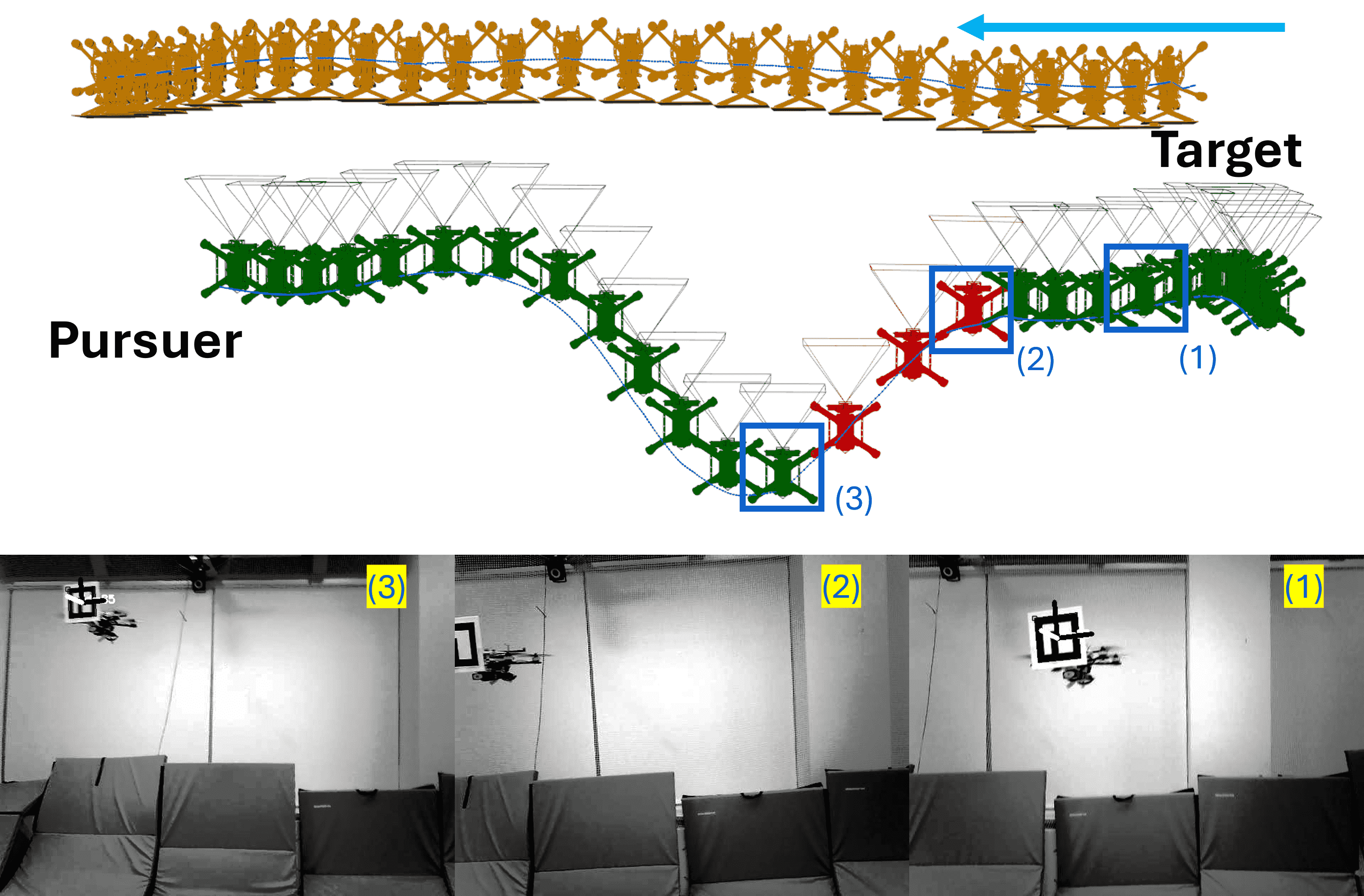
The control design is challenging because there is tension between the two goals of maintaining visual contact and gaining proximity. The pursuer may intermittently lose sight of the target because of detection failures (e.g., motion blur, lighting) or the target maneuvering outside the pursuer’s camera frame. When this happens, the pursuer has to regain visual contact by falling behind the target’s estimated position and potentially getting further away from it. A simple instance of this is shown in Figure 1.
We tackle this challenge by designing a mode switching controller [6]: in the visual tracking mode the pursuer attempts to get close to the target, and in the recovery mode it maneuvers to regain visual contact. Next, we discuss the particulars of this design, including the mode switching logic. In Section III, we will provide a general result on stability analysis of such switching controllers and in Section IV we will discuss our implementation of the controller on quadrotors.
II-A Design of Switched Visual Tracking
The position of the target () is modeled as a function of time or a trajectory in 3D-space . That is, is the position of the target at time . The Switched Visual Tracker (SVT) uses an observer that provides the relative position of the target to the pursuer (), when the target (T) is visible. This observer can be implemented using fiducial markers [11], perspective-n-point [12], or various deep learning based approaches [13, 14], and our implementation is discussed in Section IV-A. We mathematically model this camera-based observer as follows: the observer takes as input the positions of both the pursuer and the target. If the target is in view, then the observer outputs the displacement vector , otherwise, it outputs indicating that the target is not visible. We define visibility of target by the pursuer as a function which returns True when , where and is obtained by the applying the rotation matrix of the pursuer to a unit vector in z direction. It returns False otherwise. Our analysis accommodates estimation errors in but for the sake of simplifying the presentation we use the above observer model.
The visibility of the target determines the operating mode of the SVT, i.e. when the observer returns the full state of the target, the SVT will operate in visual () tracking mode and when the observer returns , the SVT will operate in the recovery () mode.
When SVT is operating in visual tracking mode, the pursuer will follow dynamic equation
where is the full state of the pursuer. The function is a tracking controller which takes as input the displacement between the target and the pursuer and generates a control input that aims to drive the pursuer to a specified offset from the target. We use standard controller design techniques for creating such a tracking controller [15].
When SVT is operating in the recovery mode, the pursuer will perform maneuver to regain visual contact to the target. It will follow dynamics equation
where is a recovery pose, from where the pursuer can see the target. The dynamics will drive the pursuer directly to the recovery pose.
II-B Computing Recovery Pose
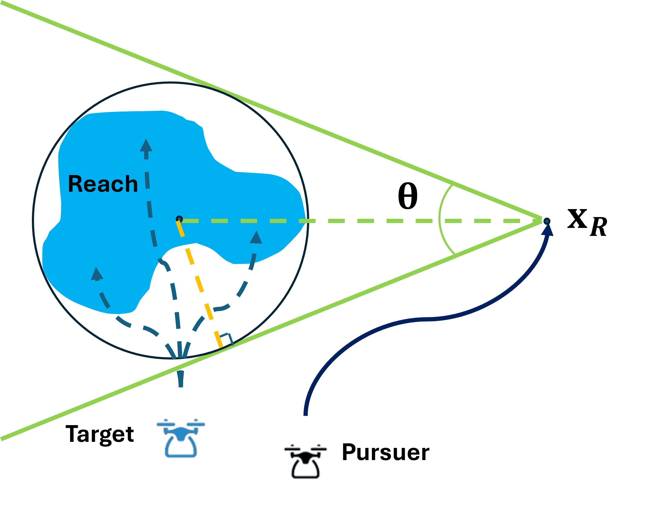
The recovery maneuver is parameterized by a time constant and has three steps: (1) the controller uses reachability analysis [16] to predict a set of positions where the target could possibly be located at starting from its last seen position ; (2) it computes a pose from which is visible, and (3) the pursuer moves to . Figure 2 shows the main idea.
In more detail, reachability analysis is a well-established technology with many available tools that can compute assuming that the target has a dynamic model , with input (or disturbance) in some range . Access to the actual dynamic model of the target is not required. The recovery point is computed so that falls within the pursuer’s camera frame, which then is guaranteed to include the target in its viewing range.
It not always possible that the pursuer can reach the computed recovery point within the recovery time , in which case the recovery maneuver would fail. We formalize the recoverability criteria as follows:
Definition 1
From initial positions of the pursuer and the target with , the system is -recoverable if the computed recovery pose is such that (1) , and (2) can reach in time .
In Section III we will assume recoverability for the analysis of SVT and in Section IV we will empirically evaluate the recoverability for our particular experimental setup.
III Stability of Target Tracking System
In this section, we will present a stability analysis of the SVT. We can view this as a switched system—a general class of dynamical systems in which an algorithm occasionally changes the plant dynamics. In SVT, the two plant dynamics or modes are the the visual and the recovery modes and the switching decision is determined by the result of . Our analysis is based on Morse and Hespanha’s Average dwell time theorem [8] which gives a stability criteria for switched systems. Roughly, that theorem (Theorem 4 of [8]) says that if the individual modes of the switched systems have decaying energy (or, more generally, Lyapunov functions ’s) and the increase in energy owing to mode switches is bounded, then the system is asymptotically stable if the rate of switching is not too high. The theorem gives the maximum allowable rate of mode switches in terms of an average dwell time, as a function of the rate of Lyapunov decay and the gains. Our Theorem 1 below slightly generalizes that result by allowing some of the individual modes to be unstable for a bounded amount of time. This is necessary for analyzing SVT because the tracking error can potentially increase in the recovery mode. We state Theorem 1 in general terms because this may be of broader interest beyond the analysis of SVT.
III-A Stability of Switching System
A switched system with a finite set of modes is described by:
| (1) |
where is the plant state at time , each describes the dynamics in mode , and is called a switching signal which chooses a particular mode for each time . The switching signal is a piece-wise constant111Strictly, its a càdlàg function with , for each . function that abstractly models the behavior of the mode switching logic as a function of time. The discontinuities in are called switching times.
Fixing a switching signal and an initial state uniquely defines a solution or an execution of the switched system which we denote by (suppressing the dependence on and ). We refer the reader to [6] for the mathematical definition of solution of switched systems. An execution of the switched system is asymptotically stable with respect to a set 222The reason why it’s converging to instead of 0 will be discussed in Theorem 1. if converges to as . The switched system is globally asymptotically stable with respect to if , all the executions are asymptotically stable. We say a mode is asymptotically stable if the subsystem is globally asymptotically stable. That is, if the switched system stays forever in mode then its solutions converge to 0. Let the be the set of asymptotically stable modes.
The standard method for proving stability of dynamical systems is to construct or find a Lyapunov function as defined below.
Definition 2
A function is a Lyapunov function for mode if there exists two class functions and such that
| (2) |
| (3) |
III-B Average Stable Dwell Time
Let us denote the number of transitions that makes in a time by . A switching signal has average dwell time if there exists integer such that for any interval
That is, such a switching signal allows for at most one mode switch in every and an additional burst of switches.
Let the number of transitions to any asymptotically stable mode over the interval be denoted by , and the total amount of time spent in stable modes be . A switching signal has average stable dwell time , if there exists integer such that for any interval
| (4) |
Compared with , imposes no constraint on the unstable modes.
III-C Stability Analysis
The visual target tracking system can be described by a class of switching system with a specific type of switching signal that alternating between visual tracking modes in and recovery modes in . Without loss of generality, assume , then all switching signals generated by satisfy that and , . The sequence of switching times is given by where is the switching time from mode to mode . Here we provide stability analysis of this class of system.
Theorem 1
Suppose we have a collection of Lyapunov functions , and there exists , such that for any even switch times ,
| (5) |
Then, for any , for any switching signal with satisfy
| (6) |
the the system is asymptotically stable with respect to
| (7) |
Proof:
We provide a sketch of the proof here. From (3) and (5), if we keep unrolling the lyapunov function value at any time , we can get
| (8) |
where we shorten as and as . Using definition of (4), and (6):
which goes to 0 as goes to infinity.
Since in between time interval , there are switches from unstable mode to stable modes, according to (4), we know for all k. Then
which converges to as goes to infinity. This gives
∎
In the visual tracking problem, the state represents the difference between the target and the pursuer, which converges to a bounded set as per (7). The Lyapunov function is defined by the distance between them, and assumption (5) describes the increase in this distance when the SVT is in recovery mode. If the pursuer is recoverable, a recovery state exists, and the pursuer can reach within , ensuring the distance increase is bounded and the assumption (5) is satisfied. The parameters in Theorem 1 have physical meanings in this context: represents the convergence rate of the pursuer in visual tracking mode, while and jointly define the maximum distance increase during recovery. In the next section, we demonstrate how this theorem guides the parameter design for the SVT.
IV Experimental Evaluation
We implemented SVT on an Agilicious drone [1] and we will evaluate its performance in following various target trajectories of a second drone. We use average tracking error (AE) (i.e., the displacement between the target and pursuer minus the tracking offset), and the Fraction of time the target is visible (FTV) from the pursuer as the two key performance metrics, which correspond to the proximity and the visibility requirements (recall the problem definition in Section II). We study overall effectiveness of SVT compared with a baseline visual tracking algorithm and how various parameters influence the performance metrics.
IV-A Experimental Setup
Target Drone
The target drone (Figure 3) is built using a 6” quadrotor frame. It carries a Raspberry Pi 3® and Navio2® for onboard computation. The target drone implements a trajectory tracking controller from [17] and is capable of following a range of pre-scripted trajectories at different speeds.
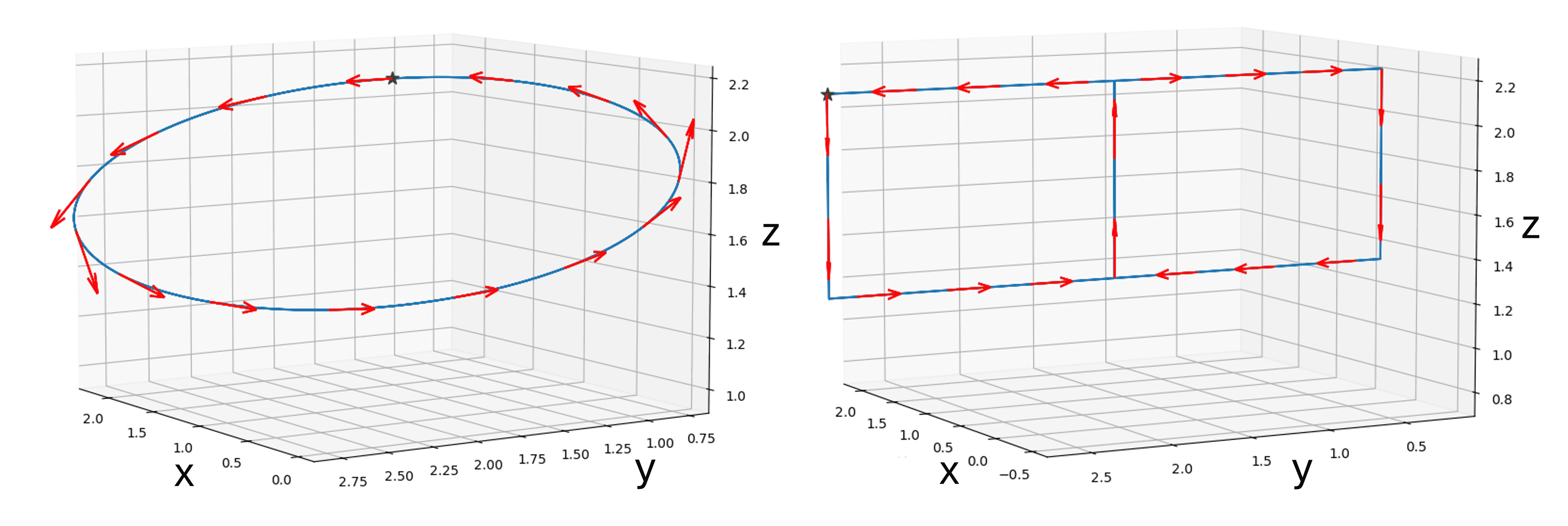
Experiments are carried out in a workspace of volume. Although SVT can track arbitrary trajectories, to create difficult, safe, and repeatable scenarios, we experiment with the target moving parallel to the pursuer’s image plane (This leads to frequent loss of sight and recoveries). Here we discuss two target trajectories Ellip and SLem in the yz-plane with no movement in the x direction (Fig. 4) and three tracking offsets (1.0m, 1.5m and 2.0m), which provides 6 scenarios called: Ellip-1.0, SLem-1.5, etc.

Pursuer Drone
The pursuer (Figure 3) is built based on Aigilicious platform [1], which uses a Nvidia Jetson TX2® as the main computer, an Intel RealSense T265® for localization, and an Arducam B0385 monocular camera for target detection. The Arducam can run at 100fps for 640x480 resolution images and has a horizontal field of view of .
SVT runs entirely on the Jetson. The observer in SVT uses an ArUco marker [11] on the target and a detection algorithm [18] running on the pursuer’s camera images which gives a relatively accurate estimate of the relative position of the target, when it is visible. A Kalman filter is used to smooth target’s position and velocity estimates.
An MPC controller [15] is used by SVT as the tracking controller in the visual tracking mode and to drive the pursuer to in the recovery mode.
To compute the recovery pose , we assume the target follows a double integrator dynamics, with acceleration in range. Reachability analysis is performed using Verse [19] to compute . We validated empirically that with these parameters and the system is -recoverable (Definition 1). A general study of recoverability gets into pursuer-evader games and is beyond the scope of this work.
Three parameters in the implementation of the SVT are significant: (1) The tracking speed () of the pursuer in visual tracking mode, which determines in Theorem 1, is set by limiting the pursuer’s x velocity. (2) The maximum recovery distance () measure the maximum change in x dimension for the pursuer in recovery mode over each run of scenario. The value represent the increase of lyapunov function in in Theorem 1. (3) The average stable dwell time () is one of the essential parameter in Theorem 1 for controlling the tracking performance. We let and is measured by where k is the number of switches from recovery mode to visual tracking mode in a scenario run. In this set of experiment, reflects how long pursuer have vision of target () and how frequent the pursuer lose visual contact of target ().
Note that we don’t have control over the and . However, we can measure these values empirically and observe their effect on the tracking performance.
IV-B Effectiveness of Tracking Algorithm
We first compare SVT against a baseline tracking algorithm, which only follows the target when it is in sight. We run all 6 scenarios with both algorithms with () 1m/s. For each algorithm, we run each scenario 4 times, take the average of the metrics, and report the results in Table I.
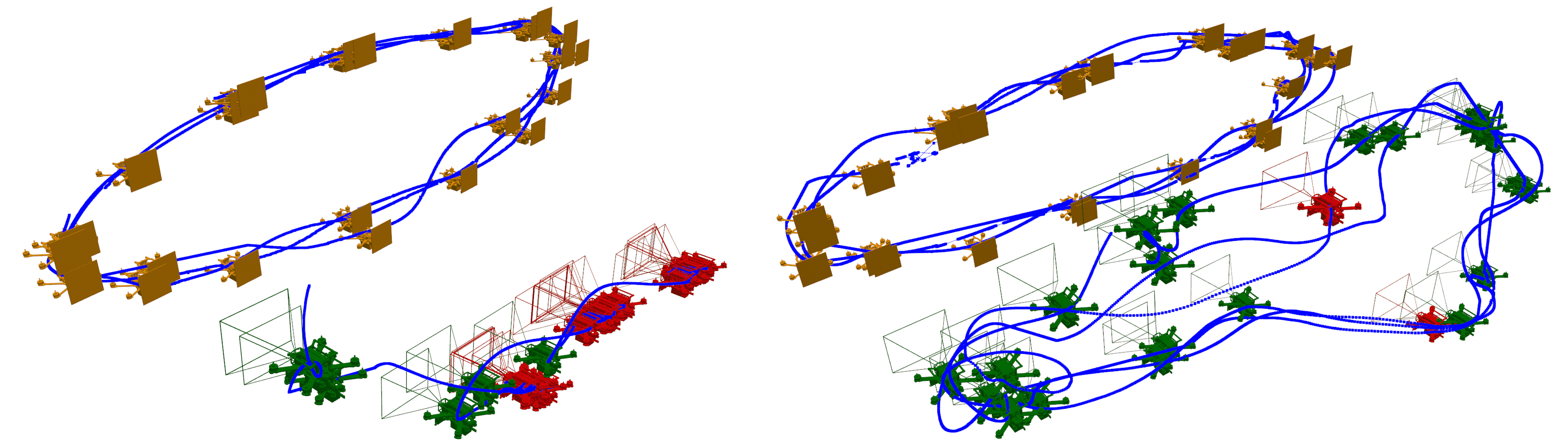
The results show that SVT achieves a better fraction of time visible in all scenarios and lower average tracking error in all but SLem-1.0. In Ellip-1.0, the average tracking error between the target and pursuer is reduced up to 45%. This clearly indicate that the SVT helps the pursuer track the target more effectively than the baseline. Fig. 5 illustrates example runs for Ellip-1.0, where the baseline fails to maintain tracking while SVT successfully follows the target’s motion. Moreover, as tracking distance decreases and the leader trajectory becomes more complex, the improvement with SVT becomes more obvious.
| SC | AE SVT | AE Base | FTV SVT | FTV Base |
|---|---|---|---|---|
| Ellip-1.0 | 0.54 | 0.98 | 85.8% | 25.3% |
| Ellip-1.5 | 0.42 | 0.56 | 93.9% | 52.0% |
| Ellip-2.0 | 0.36 | 0.34 | 98.7% | 84.7% |
| SLem-1.0 | 1.80 | 1.29 | 43.0% | 5.2% |
| SLem-1.5 | 0.80 | 0.84 | 65.5% | 27.2% |
| SLem-2.0 | 0.33 | 0.33 | 96.2% | 88.3% |
IV-C Tracking Rate and Performance Tradeoff
We explore the effect of on the tracking performance. As Theorem 1 indicates, reducing lowers , causing the system to converge more slowly to the set . Consequently, must increase to maintain tracking performance or it will degrade.
Following this guidance, we ran scenarios Ellip-1.0 and SLem-1.5 with varying . Each parameter setting was tested 4 times, and the metrics were averaged. The results in Table II show that as decreases, average tracking error increases, while the fraction of time visible remains largely unaffected, confirming our hypothesis.
However, in practice, cannot be made arbitrarily large. Our experiments show that excessively high can cause movement overshoot and rapid pitch changes in the pursuer, which can reduce tracking performance.
| SC | AE | FTV | |
|---|---|---|---|
| Ellip-1.0 | 0.1 | 1.27 | 88.3% |
| Ellip-1.0 | 0.5 | 0.66 | 84.4% |
| Ellip-1.0 | 1.0 | 0.54 | 85.8% |
| SLem-1.5 | 0.1 | 1.25 | 58.4% |
| SLem-1.5 | 0.5 | 1.07 | 47.7% |
| SLem-1.5 | 1.0 | 0.81 | 65.5% |
IV-D Recoverability-Performance Tradeoff
We examine how tracking performance is affected by , which represents the maximum increase of the Lyapunov function (5) in Theorem 1, particularly the constant . As increases, the convergence radius grows, resulting in degraded tracking performance.
In these experiments, we consider scenarios Ellip-1.0 and Ellip-1.5, running each with different to examine how affects tracking performance. The results are shown in Table III. We observe that as the maximum recovery distance increases, the average tracking error rises and the fraction of time the target is visible slightly decreases, indicating worsened tracking performance. However, cannot be set arbitrarily small; if the maximum recovery distance is too limited, finding within that range may become unfeasible, making the pursuer unable to recover from a vision loss.
| SC | AE | FTV | ||
|---|---|---|---|---|
| Ellip-1.5 | 1.0 | 1.23 | 0.43 | 91.8% |
| Ellip-1.5 | 1.0 | 1.84 | 0.52 | 87.8% |
| Ellip-1.5 | 1.0 | 1.85 | 0.51 | 89.7% |
| Ellip-1.0 | 0.5 | 2.13 | 0.56 | 86.4% |
| Ellip-1.0 | 0.5 | 2.43 | 0.66 | 83.6% |
| Ellip-1.0 | 0.5 | 2.70 | 0.74 | 82.8% |
| Ellip-1.0 | 1.0 | 1.29 | 0.48 | 87.4% |
| Ellip-1.0 | 1.0 | 1.65 | 0.52 | 85.2% |
| Ellip-1.0 | 1.0 | 2.06 | 0.63 | 84.5% |
Examining the change in , we note that, as outlined in Section II-B, the recovery pose is computed from the , which depends on the target’s initial state and the time constant . As increases, the reachable set expands, placing the recovery pose farther away and making it harder for the pursuer to reach. However, cannot be too small; if it is, the pursuer may fail to reach the recovery pose in time due to computation and hardware delays, violating the assumptions in Definition 1.
IV-E Stable Dwell Time and Performance Tradeoff
We look into how the tracking performance is influenced by . We keep as 1m/s, with the leader drone following Ellip. To isolate the impact of , we use cases where is nearly constant. The result is shown is Table IV.
| SC | AE | FTV | ||
|---|---|---|---|---|
| Ellip-2.0 | 1.63 | 44.27 | 0.407 | 98.4% |
| Ellip-1.5 | 1.69 | 9.88 | 0.412 | 94.2% |
| Ellip-1.0 | 1.65 | 3.12 | 0.515 | 85.2% |
| Ellip-1.0 | 1.67 | 3.15 | 0.548 | 86.1% |
| Ellip-1.5 | 1.21 | 12.86 | 0.411 | 95.4% |
| Ellip-1.5 | 1.34 | 9.57 | 0.412 | 93.9% |
| Ellip-1.5 | 1.23 | 6.17 | 0.426 | 91.8% |
| Ellip-1.0 | 1.29 | 3.36 | 0.479 | 87.4% |
The results show that as increases, the average tracking error decreases and the fraction of time visible increases, indicating improved overall tracking performance. A higher means the pursuer loses sight of the target less frequently or maintains visual contact for longer, naturally leading to a higher fraction of time visible. This aligns with the intuition that the system performs better with fewer losses of visual contact.
V Related Works
A challenging version of the visual tracking problem in unknown, cluttered environments is studied in [20, 21, 22]. The system developed in [22] uses trajectory prediction and a planner that combines kinodynamic search with spatio-temporal optimization to maintain safe tracking trajectories. The prediction errors arising from temporary occlusions are mitigated through high-frequency re-planning. While the experimental results are compelling, these approaches are not analytically tractable and don’t have any mechanisms for handling longer-term loss of the target. In contrast, our work explicitly addresses the challenge of vision loss by incorporating a recovery mechanism and provides stability analysis with recovery.
The problem of tracking multiple targets in a simply-connected 2D environment is studied in [23]. The approach uses a probabilistic model to generate sample trajectories that represent the likely movements of evader and construct a path for the purser that optimize the expected time to capture while ensuring guaranteed time to capture doesn’t significantly increase. The proposed recovery strategy involves systematically clearing the entire environment to ensure all regions are visible. However, this method requires the environment to be bounded and known in advance, whereas our approach does not impose specific constraints on the environment.
VI Limitations and Future Directions
We presented the design of a Switched Visual Tracker (SVT) that switches between a visual tracking and a recovery modes to effectively track moving targets that can becomes intermittently invisible. We analyzed the tracking performance of the system by extending the average dwell time theorem from switched systems theory. The proposed SVT is implemented on hardware, and its effectiveness is demonstrated through several experiments.
One limitation of the current work comes from the recoverability assumption (Definition 1). For our SVT to be recoverable, we assumed the existence of a recovery point, , and that both the computation of and the movement of the pursuer to occur within the specified time constant . The computation of used reachability analysis and did not rely on sophisticated trajectory predictions. Developing sufficient conditions for formally checking recoverability for different kinds of target trajectories, predictions, and pursuer dynamics would broaden the applicability of .
Another future direction is to extend the application of SVT to more complex environments with obstacles. Consequently, computing the recovery pose will need path planning around obstacles, adding an additional layer of challenge in the design and analysis.
References
- [1] P. Foehn, E. Kaufmann, A. Romero, R. Penicka, S. Sun, L. Bauersfeld, T. Laengle, G. Cioffi, Y. Song, A. Loquercio, and D. Scaramuzza, “Agilicious: Open-source and open-hardware agile quadrotor for vision-based flight,” AAAS Science Robotics, 2022.
- [2] J. Kim and D. H. Shim, “A vision-based target tracking control system of a quadrotor by using a tablet computer,” in 2013 International Conference on Unmanned Aircraft Systems (ICUAS), 2013, pp. 1165–1172.
- [3] A. G. Kendall, N. N. Salvapantula, and K. A. Stol, “On-board object tracking control of a quadcopter with monocular vision,” in 2014 International Conference on Unmanned Aircraft Systems (ICUAS), 2014, pp. 404–411.
- [4] I. F. Mondragón, P. Campoy, M. A. Olivares-Mendez, and C. Martinez, “3d object following based on visual information for unmanned aerial vehicles,” in IX Latin American Robotics Symposium and IEEE Colombian Conference on Automatic Control, 2011 IEEE, 2011, pp. 1–7.
- [5] H. Cheng, L. Lin, Z. Zheng, Y. Guan, and Z. Liu, “An autonomous vision-based target tracking system for rotorcraft unmanned aerial vehicles,” in 2017 IEEE/RSJ International Conference on Intelligent Robots and Systems (IROS), 2017, pp. 1732–1738.
- [6] D. Liberzon, Switching in Systems and Control, ser. Systems and Control: Foundations and Applications. Boston: Birkhauser, June 2003.
- [7] J. E. Gomez-Balderas, G. Flores, L. R. García Carrillo, and R. Lozano, “Tracking a ground moving target with a quadrotor using switching control,” Journal of Intelligent & Robotic Systems, vol. 70, no. 1, pp. 65–78, Apr 2013. [Online]. Available: https://doi.org/10.1007/s10846-012-9747-9
- [8] J. Hespanha and A. Morse, “Stability of switched systems with average dwell-time,” in Proceedings of 38th IEEE Conference on Decision and Control, 1999, pp. 2655–2660.
- [9] R. Goebel, R. G. Sanfelice, and A. R. Teel, Hybrid Dynamical Systems: Modeling, Stability, and Robustness. Princeton University Press, 2012. [Online]. Available: http://www.jstor.org/stable/j.ctt7s02z
- [10] J. Ding and C. J. Tomlin, “Robust reach-avoid controller synthesis for switched nonlinear systems,” in CDC, 2010, pp. 6481–6486.
- [11] S. Garrido-Jurado, R. Muñoz-Salinas, F. Madrid-Cuevas, and M. Marín-Jiménez, “Automatic generation and detection of highly reliable fiducial markers under occlusion,” Pattern Recognition, vol. 47, no. 6, pp. 2280–2292, 2014. [Online]. Available: https://www.sciencedirect.com/science/article/pii/S0031320314000235
- [12] S. Pan and X. Wang, “A survey on perspective-n-point problem,” in 2021 40th Chinese Control Conference (CCC), 2021, pp. 2396–2401.
- [13] J. Guan, Y. Hao, Q. Wu, S. Li, and Y. Fang, “A survey of 6dof object pose estimation methods for different application scenarios,” Sensors, vol. 24, no. 4, 2024. [Online]. Available: https://www.mdpi.com/1424-8220/24/4/1076
- [14] J. Liu, W. Sun, H. Yang, Z. Zeng, C. Liu, J. Zheng, X. Liu, H. Rahmani, N. Sebe, and A. Mian, “Deep learning-based object pose estimation: A comprehensive survey,” arXiv preprint arXiv:2405.07801, 2024.
- [15] S. Sun, A. Romero, P. Foehn, E. Kaufmann, and D. Scaramuzza, “A comparative study of nonlinear mpc and differential-flatness-based control for quadrotor agile flight,” IEEE Transactions on Robotics, vol. 38, no. 6, pp. 3357–3373, 2022.
- [16] L. Geretti, J. A. D. Sandretto, M. Althoff, L. Benet, P. Collins, M. Forets, E. Ivanova, Y. Li, S. Mitra, S. Mitsch, C. Schilling, M. Wetzlinger, and D. Zhuang, “Arch-comp23 category report: Continuous and hybrid systems with nonlinear dynamics,” in Proceedings of 10th International Workshop on Applied Verification of Continuous and Hybrid Systems (ARCH23), ser. EPiC Series in Computing, G. Frehse and M. Althoff, Eds., vol. 96. EasyChair, 2023, pp. 61–88. [Online]. Available: /publications/paper/T7LG
- [17] D. Sun, S. Jha, and C. Fan, “Learning certified control using contraction metric,” in Proceedings of the 2020 Conference on Robot Learning, ser. Proceedings of Machine Learning Research, J. Kober, F. Ramos, and C. Tomlin, Eds., vol. 155. PMLR, 16–18 Nov 2021, pp. 1519–1539. [Online]. Available: https://proceedings.mlr.press/v155/sun21b.html
- [18] G. Bradski, “The OpenCV Library,” Dr. Dobb’s Journal of Software Tools, 2000.
- [19] Y. Li, H. Zhu, K. Braught, K. Shen, and S. Mitra, “Verse: A python library for reasoning about multi-agent hybrid system scenarios,” in Computer Aided Verification, C. Enea and A. Lal, Eds. Cham: Springer Nature Switzerland, 2023, pp. 351–364.
- [20] B. Jeon, Y. Lee, and H. J. Kim, “Integrated motion planner for real-time aerial videography with a drone in a dense environment,” in 2020 IEEE International Conference on Robotics and Automation (ICRA), 2020, pp. 1243–1249.
- [21] J. Chen, T. Liu, and S. Shen, “Tracking a moving target in cluttered environments using a quadrotor,” in 2016 IEEE/RSJ International Conference on Intelligent Robots and Systems (IROS), 2016, pp. 446–453.
- [22] Z. Han, R. Zhang, N. Pan, C. Xu, and F. Gao, “Fast-tracker: A robust aerial system for tracking agile target in cluttered environments,” in 2021 IEEE International Conference on Robotics and Automation (ICRA), 2021, pp. 328–334.
- [23] N. M. Stiffler and J. M. O’Kane, “Visibility-based pursuit-evasion with probabilistic evader models,” in 2011 IEEE International Conference on Robotics and Automation, 2011, pp. 4254–4259.