Coherence and entropy complementarity relations of generalized wave-particle duality
Abstract
The concept of wave-particle duality holds significant importance in the field of quantum mechanics, as it elucidates the dual nature encompassing both wave-like and particle-like properties exhibited by microscopic particles. In this paper, we construct generalized measures for the predictability and visibility of -path interference fringes to quantify the wave and particle properties in quantum high-dimensional systems. By employing the Morozova-Chentsov function, we ascertain that the wave-particle relationship can be delineated by the average coherence. This function exhibits a close correlation with the metric-adjusted skew information, thereby we establish complementary relations between visibility, predictability, and quantum entropy, which reveals deep connections between wave-particle duality and other physical quantities. Through our methodology, diverse functions can be selected to yield corresponding complementary relationships.
I introduction
The concept of wave-particle duality (WPD), as one of the fundamental principles in Bohr’s complementarity theory, plays a pivotal role in quantum mechanics by elucidating the intrinsic disparity between the quantum realm and the classical domain Bohr1928 . Microscopic objects (such as photons, electrons, and even large organic molecules) exhibit both wave-like and particle-like behaviors when passing through an interferometer. However, these two behaviors cannot be observed simultaneously, leading to the relations of wave-particle duality. The quantitative analysis of this phenomenon was initially presented by Wootters and Zurek WotZrk and has since been extensively studied by subsequent researchers Englert1996 ; Jaeger ; GreenYas . Notably, Englert proposed the following elegant duality relation Englert1996 ,
| (1) |
where represents path information (predictability), while denotes the visibility of interference fringes in a two-path interferometer. This trade-off relation imposes limitations on the information that can be simultaneously contained within both particle and wave aspects.
The quantitative investigation of WPD in -path () interferometers was first proposed by Dürr Durr who introduced a generalized predictability measure and a generalized visibility measure . The former is determined on diagonal entries of the density matrix while the latter depends on non-diagonal elements. Subsequently, Englert et al. Englert2008 ; Durr ; TsuiKim ; Peng ; LuX refined a reasonable criteria for these two quantifiers, which requires that normalization, invariance under relabeling, and convexity be satisfied. This framework is adopted in this study to quantify wave-particles by utilizing some functions.
With the development of quantum resource theory, there are growing interests in exploring the relationship between WPD and various quantum information concepts, such as entanglement Jakob1 ; TsuiKim ; Jakob2 , coherence Bagan ; Roy ; LuoSun ; BuKF ; Bera , entropic uncertainty Coles1 ; Coles2 , and quantum state discrimination LuX . The predictability-visibility-concurrence triality relation has been experimentally and theoretically proven in Ref.Peng . The equivalence between WPD and entropic uncertainty has been explored in Coles1 . The relationship between coherence and path information has been presented in Ref.Bagan . The complementary relations between WPD and entangled monotones have been proposed and proven in Basso . The complementary relationship between WPD and mixedness in -path interferometers has been revealed in TsuiKim . Sun and Luo SunLuo1 were the first to utilize coherence for quantifying interference from the perspective of Wigner-Yanase skew information. Regarding the quantification of coherence, there have been numerous recent research studies with corresponding results. It is worth mentioning that Sun et al. Sun have quantified coherence relative to channels using metric-adjusted skew information; building upon this, Fan et al. Fan proposed an expression for average coherence while introducing a new entropy called quantum entropy. However, the idea of quantitatively studying WPD using metric-adjusted skew information has not yet been implemented in multipath interferometers, making it both novel and natural to investigate the complementary relations between WPD and quantum entropy.
In this paper, we study the quantitative relations between WPD and some quantum information measures, such as entropy and skew information. We first establish a generalized measure for quantifying the predictability and visibility properties of particles and waves in multi-path interferometers, utilizing a specialized symmetric operator concave function based on the spectral of density matrices. The function is closely associated with the metric-adjusted skew information, serving as a crucial link to establish the quantitative relation between predictability and visibility, as well as average coherence. We find that the sum of the generalized predictability and generalized visibility is less than or equal to one. Furthermore, complementary relations among predictability, visibility, and quantum entropy are revealed, and the trade-off relations are illustrated through detail examples.
II Measure of particle and wave aspects
II.1 Preliminaries
An acceptable measure of path knowledge is a continuous function of the diagonal entries of a density matrix , where stands for the diagonal part of . As a valid predictability, the function should satisfy the following criteria:
| (1a) iff for one , i.e., the path is certain. (2a) iff for all , i.e., the path is completely uncertain. (3a) is invariant under permutations of the path labels. (4a) is convex, namely, for any two density matrices and , one has for (), |
Correspondingly, the wave aspect is characterized by the off-diagonal elements of . As a well defined measure of the wave aspect, the visibility should satisfy the following conditions:
| (1b) iff . (2b) iff , i.e., is a pure state with equal diagonal elements. (3b) is invariant under permutations of the path labels. (4b) is convex. |
Concerning the general measures of the predictability and the visibility, we denote by the set of all functions such that i) for any complex positive matrices ( is operator monotone), ii) for all (symmetric), iii) (normalized), iv) (regular). For any , we consider the Morozova-Chentsov function , . The metric-adjusted skew information of with respect to an operator is defined by Hansen
| (2) |
where is the commutator of operators and . Here and are left and right multiplication operators by . For , denote
| (3) |
The metric-adjusted skew information of can be further expressed as
| (4) |
where is the corresponding generalized mean function and operator concave Pattrawut Chansangiam .
Based on the properties of the metric-adjusted skew information, an average coherence measure with respect to operator monotone function has been has proposed in Ref.Fan , which can be also interpreted as a measure of coherence for the depolarizing channel. For any -dimensional state and , the average coherence is given by
| (5) |
where , and is the spectral decomposition of .
II.2 Main results
Proposition 1.
For any -dimensional state and , the predictability ,
| (6) |
complies with the set of requirements .
The proof is given in Appendix A. Actually, the function genuinely depends on the diagonal elements of and satisfies . attains its maximal value 1 when there exists only one diagonal element 1, which is attained when is a pure state. This is consistent with the fact that the path is completely certain. When the diagonal entries of (i.e., the eigenvalues of ) are all equal, vanishes and the path information is completely uncertain. For the visibility we have the following conclusion, see Appendix B.
Proposition 2.
For any -dimensional state and , the visibility defined by,
| (7) |
complies with the set of requirements , assuming that does not increase under incoherent operations.
It’s easy to verify that . reaches its minimum 0 when (i.e., the off-diagonal entries of are all 0). Meanwhile, attains its maximal value 1 when is a pure state with equal diagonal entries, for which has non-zero off-diagonal elements. Namely, the function characterizes the influence of the off-diagonal elements on the wave aspect. Consider the von Neumann measure : . denotes the full dephasing of in the computational basis . In the following we denote the change of due to the measurement. Additionally, it is easily seen that measurements do not alter the particle properties, i.e., .
Indeed, there are many ways to construct the predictability and visibility measures that comply with the requirements and satisfy certain duality relations. Different measures and trade-off relations characterize different aspects of the wave and particle properties. Currently, these measures are mainly defined by either the elements or the spectra of a density matrix. The former requires comprehensive knowledge of the density matrix. For example, the visibility and predictability can be defined as functions of the off-diagonal and diagonal entries of the density matrix, respectively. In this paper, we adopt the latter approach to develop measures of predictability and visibility in multi-path interference without necessitating complete information about quantum states. In fact, the measures defined in these two ways are generally not equivalent. For instance, the measures with predictability and visibility cannot be expressed in the form of measures defined in this paper, since , where TsuiKim .
III Complementarity between WPD and information measures
From (5), (6) and (7) we have the following analytical relation among the predictability, visibility and the average coherence.
Theorem 1.
For any state in -dimensional quantum system and , we have
| (8) |
When is a pure state, one has and (8) reduces to . Associated to the Wigner-Yanase skew information, we take into account an operator monotone function . Then we obtain correspondingly
| (9) | |||
| (10) | |||
| (11) |
which satisfy the trade-off relation (8). In particular, for two-dimensional quantum states, (8) reduces to the following relation,
| (12) |
where is the quantum unified- entropy, (, ) for and .
Note that (12) can also be expressed in terms of the quantum Sharma-Mittal entropy MDG ,
where s are the eigenvalues of , and are two real numbers with , and . In terms of the quantum Sharma-Mittal entropy, (12) has the following form,
| (13) |
Based on the concept of average coherence, in Fan a bona fide measure of entropy , named quantum entropy, has been recently proposed,
| (14) |
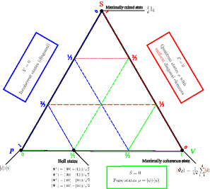
The entropy quantifies the mixing of a -dimensional quantum state , with for pure states and for maximum mixedness. For a schematic distribution of predictability , visibility and quantum entropy in quantum states , Bell states, maximally coherent state and maximally mixed state, see FIG.1 and Appendix C).
Theorem 2.
For any -dimensional state and , we have the following complementary relation between the quantum entropy and the wave-particle duality.
| (15) |
From the perspective of metric-adjusted skew information, Eq.(15) can be further represented as
| (16) |
where constitutes an operator orthonormal basis. (16) can be viewed as a complementary relation between the metric-adjusted skew information and the wave-particle duality.
Let denote the set of all complex matrices. For any , density matrices , and a function , the quasientropy is defined by Hiai ,
| (17) |
where is the Hilbert-Schmidt inner product and refers to the linear mapping defined by . Since the quantum entropy and the quasientropy have the following relation Fan ,
| (18) |
a series of complementary relations can be established among the predictability, visibility and quasientropy,
| (19) |
In particular, for we have . As a direct consequence of the Theorem 2 and the properties of quantum entropy, we have
Corollary. For any -dimensional state and , the corresponding predictability and visibility satisfy
| (20) |
| convex | convex | concave |
Remark The quantum entropy of a state is defined by , where is a monotonic functional and is continuous satisfying either (i) is strictly concave and is strictly increasing or (ii) is strictly convex and is strictly decreasing Bosyk . Denote . Although in Eq.(6) seems to be of the form of with , it fails to satisfy the conditions of a quantum entropy (it satisfies the convexity requirement on predictability). Nevertheless, when we consider the strictly increasing function , the quantum entropy here gives rise to the following complementary relation with the predictability and visibility,
| (21) |
In conjunction with Theorem 2, the connection between quantum entropy and quantum entropy is also revealed in this way.
Example 1.
In the computational basis , we consider the qubit state in the Bloch representation:
where , I is the identity operator, and , and are the Pauli matrices. Let be the module of the Bloch vector of . The eigenvalues of are and . Meanwhile, the two eigenvalues of are given by and . Therefore, by direct calculation we have
| (22) | ||||
The pure states with achieve the maximal visibility. In Table I we list the formulas if the function , the mean , the predictability, visibility and quantum entropy for qubit state in Example 1, where QFI, WY and SLD stand for quantum Fisher information, Wigner-Yanase skew information and symmetric logarithmic derivative Sun , respectively.
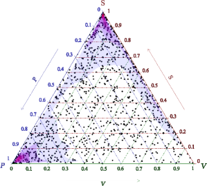
Concerning the complementarity described by Eq.(22) for any qubit state, FIG.2 shows the numerical results on the proportion of , and distributions, which are randomly generated by the Mathematica software.
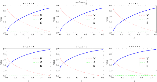
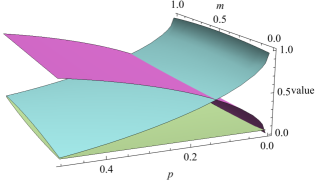
Example 2.
We consider the Werner states
on the -dimensional Hilbert space , where is the flip operator with an orthonormal basis of . W has the following spectral decomposition Li ,
with eigenvalues of multiplicities and , respectively. The eigenvalues of are and of multiplicities and , respectively. Here is projection onto the symmetric (antisymmetric) subspace of , and . We have
| (23) | ||||
IV Conclusions
Based on an arbitrary symmetric normalized regular operator monotone function , we have constructed quantitative measures of particle and wave aspects respectively. Inherently, we have investigated the relationship between the wave-particle duality and the quantum coherence associated with the metric-adjusted skew information. We have also established the trade-off relations between the wave-particle duality and the quantum entropy. Our results reveal the profound relations among the predictability, visibility and quantum coherence, and may highlight further investigations on relations between WPD and other quantum quantities such as entanglement and non-localities.
ACKNOWLEDGMENTS
This work is supported by the National Natural Science Foundation of China (NSFC) under Grant No. 12075159 and No. 12171044, and the specific research fund of the Innovation Platform for Academicians of Hainan Province.
Appendix A Proof of the Proposition 1
To prove proposition 1, consider the spectral decomposition of , . In Ref.Hansen it has been proven that the trace of is given by
| (A1) |
and the equality holds if and only if is a pure state. Firstly, is equivalent to . If there is one such that , which implies that has only one eigenvalue of 1 and the rest is 0. Thus is pure. The converse is obvious. Therefore if and only if for one .
Secondly, is equivalent to . Let be the nonzero eigenvalues of satisfying . For any , where the equality holds if and only if . Hence, , and the last equality is saturated if and only if . Thus if and only if .
For item (3a), the permutation of the diagonal entries of density matrix (i.e., the eigenvalues of ) does not alter the value of .
Finally, it is known that if is a continuous convex function, then the trace function is a convex function, see Klien , and the combination of is an operator concave function proves that is convex. This concludes the proof.
Appendix B Proof of the Proposition 2
Here we provide the proof of Proposition 2. Firstly, we just need to prove that when . We invoke generalized Klien’s inequality Klien on differentiable convex functions. For all Hermitian matrices , and all differentiable convex functions :
| (B1) |
If is strictly convex, the equality holds if and only if . Combined with and , this implies that
| (B2) | |||||
Therefore if and only if .
For item (2b), , which is equivalent to , implies that is a pure state. This is because if is not a pure state, then has at least two different nonzero eigenvalues . We have
This is impossible. So and . Therefore, for all . On the other hand, if is a pure state with equal diagonal elements, it is evident from the proof of Proposition 1 that and . Thus .
For item (3b), it is evident that is invariant under permutations of the path labels.
Finally, we need to show the convexity of . Considering the -dimensional quantum state , and . We suppose and () are eigenvalues of and , then the eigenvalues of are . Thus,
where the first and third equalities come from the definition of . The second equality holds since for any . Similarly,
Thus we have
| (B4) | |||||
Suppose the are states of a system . We introduce an auxiliary system whose state space has an orthonormal basis and . Assume that the initial joint state of is:
where and . We consider an incoherent operation on the whole system with Kraus operators . Then . We have Nielsen2000
| (B5) |
By definition we can easy to know that
| (B6) | |||||
Due to Eq.(B4) and the monotonicity of under incoherent operation, we obtain
| (B7) | |||||
from which item (4b) follows.
Appendix C Basic properties of quantum entropy
Quantum entropy defined by Eq.(14) has the following properties, which can be directly verified Fan .
-
(i)
is non-negative. The quantum entropy is zero if and only if the state is pure.
-
(ii)
In a -dimensional Hilbert space, the quantum entropy is at most . The entropy is equal to if and only if the system is in the completely mixed state .
-
(iii)
Suppose a composite system is in a pure state , then , where and .
-
(iv)
is concave, i.e., , where are probabilities.
-
(v)
is unitary invariant, i.e., .
-
(vi)
.
-
(vii)
, where are probabilities, are orthogonal states for a system , and are quantum states on another system .
References
- (1) N. Bohr, The quantum postulate and the recent development of atomic theory, Nature 121, 580-590 (1928).
- (2) W. K. Wootters and W. H. Zurek, Complementarity in the doubele-slit experiment: Quantum nonseparability and a quantitative statement of Bohr’s principle, Phys. Rev. D 19, 473 (1979).
- (3) D. M. Greenberger and A. Yasin, Simultaneous wave and particle knowledge in a neutron interferometer, Phys. Lett. A 128, 391 (1988).
- (4) G. Jaeger, A. Shimony and L. Vaidman, Two interferometric complementarities, Phys. Rev. A 51, 54 (1995).
- (5) B. G. Englert, Fringe visibility and which-way information: an inequality, Phys, Rev. Lett. 77, 2154 (1996).
- (6) S. Dürr, Quantitative wave-particle duality in multibeam interferometers, Phys. Rev. A 64, 042113 (2001).
- (7) X. Peng, X. Zhu, D. Suter, J. Du, M. Liu and K. Gao, Quantification of complementarity in multiqubit systems, Phys. Rev. A 72, 052109 (2005).
- (8) B. G. Englert, D. Kaszlikowsk, L. C. Kwek and W. H. Chee, Wave-particle duality in multi-path interferometers: general concepts and three-path interferometers, Int. J. Quantum Inf. 06, 129 (2008).
- (9) X. Lü, Quantitative wave-particle duality as quantum state discrimination, Phys. Rev. A 102, 022201 (2020).
- (10) Y. T. Tsui, Sunho Kim, Generalized wave-particle-mixdness triality for -path interferometers, Phys. Rev. A 109, 052439 (2024).
- (11) M. Jakob and J. A. Bergou, Complementarity and entanglement in bipartite qubit systems, Phys. Rev. A 76, 052107 (2007).
- (12) M. Jakob and J. A. Bergou, Quantitative complementarity relations in bipartite systems: entanglement as a physical reality, Opt. Commun. 283, 827 (2010).
- (13) M. N. Bera, T. Qureshi, M. A. Siddiqui and A. K. Pati, Duality of quantum coherence and path distinguishability, Phys. Rev. A 92, 012118 (2015).
- (14) E. Bagan, J. A. Bergou, S. S. Cottrell and M. Hillery, Relations between coherence and path information, Phys. Rev. Lett. 116, 160406 (2016).
- (15) S. L. Luo and Y. Sun, Coherence and complementarity in state channel interaction, Phys. Rev. A 98, 012113 (2018).
- (16) K. F. Bu, L. Li, J. D. Wu and S. M. Fei, Duality relation between coherence and path information in the presence of quantum memory, J. Phys, A: Math. Theor. 51, 085304 (2018).
- (17) P. Roy and T. Qureshi, Path predictability and quantum coherence in multi-slit interference, Phys. Scr. 94, 095004 (2019).
- (18) P. J. Coles, J. Kaniewski and S. Wehner, Equivalence of wave-particle duality to entropic uncertainty, Nat. Commun. 5, 5814 (2014).
- (19) P. J. Coles, Entropic framework for wave-particle duality in multipath interferometers, Phys. Rev. A 93, 062111 (2016).
- (20) M. L W Basso and J. Maziero, Entanglement monotones from complementarity relations, J. Phys, A: Math. Theor. 55, 355304 (2022).
- (21) Y. Sun and S. Luo, Quantifying interference via coherence, Ann. Physik 533, 2100303 (2021).
- (22) Y. Sun, N. Li, and S. L. Luo, Quantifying coherence relative to channels via metric-adjusted skew information, Phys. Rev. A 106, 012436 (2022).
- (23) Y. J. Fan, N. Li, and S. L. Luo, Average coherence and entropy, Phys. Rev. A 108, 052406 (2023).
- (24) F. Hansen, Metric adjusted skew information, Proc. Natl. Acad. Sci. USA 105, 9909-9916 (2008).
- (25) P. Chansangiam, Operator monotone functions: characterizations and integral representations, arXiv:1305.2471 [math.FA].
- (26) F. Hiai and D. Petz, From quasi-entropy to various quantum in formation quantities, Publ. Res. Inst. Math. Sci. 48, 525 (2012).
- (27) S. Mazumdar, S. Dutta, and P. Guha, Sharma-Mittal quantum discord, Quantum Inf Process 18, 169 (2019).
- (28) G. M. Bosyk, S. Zozor, F. Holik, M. Portesi, and P. W. Lamberti, A family of generalized quantum entropies: definition and properties, Quantum Inf Process 15, 3393 (2016).
- (29) N. Li, S. L. Luo, and Y. Sun, Information-theoretic aspects of Werner states, Ann. Phys. (NY) 424, 168371 (2021).
- (30) Eric A. Carlen, Trace inequalties and quantum entropy: An introductory course, Contemp. Math. 529:73-140 (2010).
- (31) M. A. Nielsen and I. L. Chuang, Quantum Computation and Quantum Information. Cambridge University Press, Cambridge, 2000.