A close outer companion to the ultra-hot Jupiter TOI-2109 b? ^,

Abstract

Context. Hot Jupiters with close-by planetary companions are rare, with only a handful of them having been discovered so far. This could be due to their suggested dynamical histories, leading to the possible ejection of other planets. TOI-2109 b is special in this regard because it is the hot Jupiter with the closest relative separation from its host star, being separated by less than 2.3 stellar radii. Unexpectedly, transit timing measurements from recently obtained CHEOPS observations show low amplitude transit-timing variations (TTVs).

Aims. We aim to search for signs of orbital decay and to characterise the apparent TTVs, trying to gain information about a possible companion.

Methods. We fit the newly obtained CHEOPS light curves using TLCM and extract the resulting mid-transit timings. Successively, we use these measurements in combination with TESS and archival photometric data and radial velocity data to estimate the rate of tidal orbital decay of TOI-2109 b, as well as characterise the TTVs using the N-body code TRADES and the photodynamical approach of PyTTV.

Results. We find tentative evidence at $3\sigma$ for orbital decay in the TOI-2109 system, when we correct the mid-transit timings using the best-fitting sinusoidal model of the TTVs. We do not detect additional transits in the available photometric data, but find evidence towards the authenticity of the apparent TTVs, indicating a close-by, outer companion with $P_{\mathrm{c}}>1.125\,$d. Due to the fast rotation of the star, the new planetary candidate cannot be detected in the available radial velocity (RV) measurements, and its parameters can only be loosely constrained by our joint TTV and RV modelling.

Conclusions. TOI-2109 could join a small group of rare hot Jupiter systems that host close-by planetary companions, only one of which (WASP-47 b) has an outer companion. More high-precision photometric measurements are necessary to confirm the existence of this planetary companion.

1 Introduction

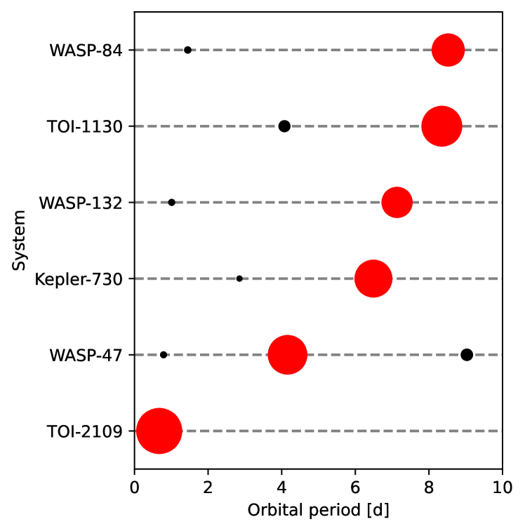
Figure 1: Overview of hot Jupiters (red) with close-by companions (black), including TOI-2109 b. Sizes given to scale. We note that the WASP-47 system also contains a long-period companion that is not shown here. System parameters taken from Cañas et al. (2019); Wong et al. (2021); Hord et al. (2022); Korth et al. (2023); Maciejewski et al. (2023); Nascimbeni et al. (2023).

There are more than 500 hot Jupiter (HJ) systems known, only a few of which are known to host close-by planetary companions. These are WASP-47 (Hellier et al., 2012; Becker et al., 2015; Neveu-VanMalle et al., 2016; Nascimbeni et al., 2023), Kepler-730 (Thompson et al., 2018; Zhu et al., 2018; Cañas et al., 2019), TOI-1130 (Huang et al., 2020; Korth et al., 2023), TOI-1408 (Galazutdinov et al., 2023; Korth et al., 2024), WASP-132 (Hellier et al., 2017; Hord et al., 2022), and WASP-84 (Anderson et al., 2014; Maciejewski et al., 2023). The HJs in these systems all host only inner companions in the Earth- to Neptune-regime, except for WASP-47, which also contains a close outer sub-Neptune companion to the HJ, and a long-period giant planet. An overview of these systems is given in Fig. 1. Other systems worth mentioning are TOI-2000 (Sha et al., 2023), containing a hot Saturn with an inner companion, TOI-5398 (Mantovan et al., 2024), hosting a warm Saturn with an inner sub-Neptune, and WASP-148 (Hébrard et al., 2020), consisting of a hot Saturn and a non-transiting misaligned outer Saturn, near a 4:1 mean-motion resonance (MMR). Furthermore, a recent study by Wu et al. (2023) finds that at least $12\%\pm 6\%$ of hot Jupiters should have close-by companions, according to their analysis of the full Kepler data set. This indicates that there should be more of these hitherto rare systems within the sample of known hot Jupiter systems.

Theories for the origins of hot Jupiters include in situ formation, disk migration and high-eccentricity tidal migration (for a review see e.g. Dawson & Johnson 2018). As found by Rice et al. (2022), the distributions of obliquities and eccentricities that have been observed, are consistent with high-eccentricity migration and tidal damping, and do not strictly require in situ formation or disk migration. Due to strong tidal interactions with their host star, misalignments and eccentricities can be damped relatively quickly, effectively erasing the imprints of formation and migration. However, this only applies to hot Jupiters orbiting cool stars, since tidal interactions are less efficient for hot host stars, as has been observed by Albrecht et al. (2021). A recent review on stellar obliquities is given by Albrecht et al. (2022). Violent migration scenarios, like planet-planet scattering, make it hard to explain close planetary companions to hot Jupiters. A study on in situ formation using N-body simulations, focussed on hot Jupiters with companion super-Earths, found that they can produce such systems, obtaining similar occurrence rates for hot Jupiters with inner companions, but according to their simulations, hot Jupiters should not be detected as single transiting planets as often. A fraction of their simulations also led to two close-in gas giants (Poon et al., 2021).

Close-by planetary companions, especially when in resonance, can induce strong transit timing variations (TTVs) on one another, see e.g. Nascimbeni et al. (2023) for a dynamical modeling of the WASP-47 system, making use of high-precision CHEOPS photometry. A few other prominent examples of the effect of TTVs are the Kepler-9 system (Holman et al., 2010), Kepler-80 (MacDonald et al., 2016), TRAPPIST-1 (Gillon et al., 2017; Grimm et al., 2018), and TOI-178 (Leleu et al., 2021). Examining TTVs has the potential to deliver more information about the observed system, like constraining planetary masses or orbital periods of non-transiting companions (Lithwick et al., 2012; Wu & Lithwick, 2013; Hadden & Lithwick, 2014, 2017).

Tidal orbital decay is caused by gravitational interactions of a planet with its host star. These interactions raise a bulge on the surface of the star, which can lead to the transfer of angular momentum between the two bodies. Orbital decay only happens if the star is rotating more slowly than the planet is orbiting around the star in the case of spin-orbit alignment because the tidal bulge will be dragged behind the moving sub-planetary point on the stellar surface. Consequently, the planetary orbit shrinks, while the star spins up (Counselman, 1973; Rasio et al., 1996). There is always an offset between the position of the stellar bulge and the sub-planetary point due to the viscosity of the plasma, except if the orbital period of the planet and the rotation of the star are synchronised (see e.g. Hut 1981). Even outward migration of the planet is possible, if the star is rotating faster than the planet is orbiting. A measure of the efficiency of the dissipation of orbital kinetic energy due to friction within the star, in the case of tidal orbital decay, is given by the modified stellar tidal quality factor $Q^{\prime}_{\star}$ (Goldreich & Soter, 1966). Theory suggests values ranging from 10⁵ to 10⁹ for stars, with smaller values indicating a higher dissipation efficiency (see e.g., Meibom & Mathieu 2005; Jackson et al. 2008; Ogilvie & Lin 2007; Penev & Sasselov 2011; Husnoo et al. 2012; Penev et al. 2012; Ogilvie 2014; Collier Cameron & Jardine 2018). Penev et al. (2018) treated $Q^{\prime}_{\star}$ as being dependent on the tidal forcing period rather than being a constant for different stellar types, and found $Q^{\prime}_{\star}$ in the range from $10^{5}$ to $10^{7}$ for orbital periods between 0.5 days and 2 days. Measurements of $Q^{\prime}_{\star}$ from WASP-12 b and Kepler-1658 b give values of $Q^{\prime}_{\star}=1.8\times 10^{5}$ (Yee et al., 2020) and $Q^{\prime}_{\star}=2.5\times 10^{4}$ (Vissapragada et al., 2022), respectively, where the host star of the latter is a subgiant. Additionally, several lower limits for $Q^{\prime}_{\star}$ were established in systems where tidal orbital decay could not be confirmed yet (see e.g., Maciejewski et al. 2020; Patra et al. 2020; Barros et al. 2022; Grunblatt et al. 2022; Ivshina & Winn 2022; Rosário et al. 2022; Harre et al. 2023; Wang et al. 2024).

TOI-2109 is a fast-rotating ($v\sin i=(81.2\pm 1.6)$ km s^-1) F-type star, with a mass of $M_{\star}=1.447^{+0.075}_{-0.078}\,M_{\odot}$ and a radius of $R_{\star}=1.698^{+0.062}_{0.057}$ (Wong et al., 2021). It hosts an ultra-hot Jupiter, TOI-2109 b, in a tight $P=0.672\,$d orbit, making it the shortest orbital period hot Jupiter orbiting a Sun-like star, with a separation of less than 2.3 stellar radii from the center of its star (Wong et al., 2021). Its predicted orbital decay rate is one of the highest amongst all hot Jupiters (see Fig. 14 of Wong et al. 2021), hence making this planet a very interesting target for orbital decay studies. However, the fast rotation of the stellar host impacts the expected magnitude of the orbital decay signature due to the small difference of rotation period and orbital period, which, in combination with the shallower convective zones of these stars, might lead to less efficient tidal interactions (see e.g. Boué & Efroimsky 2019; Harre et al. 2023). Its equilibrium temperature is the second highest of all known exoplanets with $T_{\mathrm{eq}}=3646\pm 88\,$K, being slightly cooler than KELT-9 b with $T_{\mathrm{eq}}=3921^{+182}_{-174}$ (Gaudi et al., 2017; Jones et al., 2022). Contrary to many other hot Jupiters orbiting hot stars, TOI-2109 b is aligned ($\lambda=1.7^{\circ}\pm 1.7^{\circ}$). Yet, the stellar effective temperature is not far off the Kraft break (Kraft, 1967) at $T_{\mathrm{eff}}=6530^{+130}_{-120}\,$K.

CHEOPS (CHaracterising ExOPlanet Satellite) is an S-class mission of the European Space Agency (ESA), dedicated for photometric follow-up of transiting planets of bright stars (Benz et al., 2021). With its defocused 32 cm telescope, it delivers high-precision photometry, which is able to precisely constrain planetary radii (e.g. Benz et al. 2021; Deline et al. 2022). We observed TOI-2109 under the “Tidal decay (ID 0012)” and the “TIDES (ID 0063)” programmes, the first of which is dedicated to observing hot Jupiters for measurements of tidal orbital decay as part of the Guaranteed Time Observing (GTO) programme of CHEOPS (Barros et al., 2022), with the latter being part of the first extension of the CHEOPS mission. CHEOPS’ performance and its potential for the characterisation of ultra-hot Jupiters have been demonstrated in (Lendl et al., 2020).

In this paper, we present new transit and phase curve observation of TOI-2109 b, taken with the CHEOPS space telescope, and analyse the apparent transit timing variations. In Sect. 2, we describe the observations that were used consecutively in our light curve analysis (Sect. 3), orbital decay analysis (Sect. 4), and TTV analysis (Sect. 5). The conclusions are presented in Sect. 6.

2 Observations

TOI-2109 was observed by CHEOPS in 31 visits, eight of which were phase curve observations, with the rest having been transit observations. Details, including file keys for data access, can be found in Table 1. These data can be accessed via the DACE (Data & Analysis Center for Exoplanets) website of the University of Geneva, via the CHEOPS archive, via the PYCHEOPS Python package (Maxted et al., 2022) using the provided file keys, or at the CDS. We fully process this data ourselves.

In addition to observations by CHEOPS, TOI-2109 has also been observed in two TESS Sectors, 25 and 52 (Cycle 2 and 4). However, only the latter is available at a cadence of 120 s, with the first being extracted from the full frame images FFIs), resulting in a cadence of 30 min. We fit these light curves to derive the mid-transit times.

Furthermore, Wong et al. (2021) took 20 (partial) transit observations with ground-based telescopes. These include observations from the Fred Lawrence Whipple Observatory with KeplerCam, the University of Louisville Manner Telescope, the Maury Lewin Astronomical Observatory, MuSCAT2 with TCS at Teide Observatory, MuSCAT3 with FTN at Haleakala Observatory, the Wild Boar Remote Observatory, the Grand-Pra Observatory with the RCO, and the Las Cumbres Observatory Global Telescope network using the telescopes of the McDonald observatory, Siding Spring Observatory, South African Astronomical Observatory and the Cerro Tololo Interamerican Observatory. Aside from photometric observations, Wong et al. (2021) also published a total of 58 measured radial velocities (RVs) from TRES and FIES, contributing 47 (including 28 from transit spectroscopy observations) and 11, respectively. For these data, we use the derived timings and RVs as provided by Wong et al. (2021).

Besides these data, TOI-2109 was also observed by several cameras of SuperWASP-N (Pollacco et al., 2006) from 2006 to 2011, giving us early photometry for our orbital decay analysis. After phase-folding, the transit is clearly visible. We fully process this data ourselves.

Table 1: Log of CHEOPS observations of TOI-2109.

Visit no.	Start date	Duration	No. of data	Eff.	File key
	[UTC]	[h]	points	[$\%$]
1	2021-05-14 22:35:37	5.29	249	78.3	CH_PR100012_TG002001_V0300
2	2021-05-18 23:00:37	5.62	275	81.3	CH_PR100012_TG002002_V0300
3	2021-05-21 15:55:17	5.44	260	79.5	CH_PR100012_TG002003_V0300
4	2021-05-27 17:00:17	5.42	255	78.2	CH_PR100012_TG002004_V0300
5	2021-05-31 01:40:37	5.64	301	88.7	CH_PR100012_TG002101_V0300
6	2021-06-04 02:36:18	5.64	305	89.9	CH_PR100012_TG002102_V0300
7	2021-06-10 19:44:37	5.64	277	81.7	CH_PR100012_TG002103_V0300
8	2021-06-12 04:36:17	5.95	276	77.1	CH_PR100012_TG002104_V0300
9	2021-06-13 12:33:36	5.60	302	89.6	CH_PR100012_TG002105_V0300
10	2021-06-16 04:50:17	5.64	264	77.8	CH_PR100012_TG002106_V0300
11	2022-04-10 19:21:38	5.54	231	69.3	CH_PR100012_TG002601_V0300
12	2022-04-16 04:03:18	5.64	206	60.7	CH_PR100012_TG002602_V0300
13	2022-04-25 14:24:38	6.44	263	67.9	CH_PR100012_TG002603_V0300
14	2022-05-30 13:29:38	5.59	294	87.5	CH_PR100012_TG003301_V0300
15	2022-05-31 05:32:18	5.64	273	80.5	CH_PR100012_TG003302_V0300
16	2022-05-31 21:41:38	5.69	303	88.6	CH_PR100012_TG003303_V0300
17	2022-06-02 06:13:18	5.45	260	79.2	CH_PR100012_TG003304_V0300
18	2022-06-02 22:18:38	5.59	301	89.5	CH_PR100012_TG003305_V0300
19	2022-06-06 06:37:38	5.64	276	81.4	CH_PR100012_TG003306_V0300
20	2022-06-12 07:53:18	5.64	268	79.0	CH_PR100012_TG003307_V0300
21	2023-04-15 00:10:19	5.62	235	69.5	CH_PR140063_TG000101_V0300
22	2023-04-21 01:29:19	5.34	220	68.5	CH_PR140063_TG000102_V0300
23	2023-04-27 02:37:19	5.25	210	66.4	CH_PR140063_TG000103_V0300
24	2023-05-13 07:50:19	23.74	1042	73.1	CH_PR100012_TG003901_V0300
25	2023-05-17 21:41:59	26.00	1165	74.6	CH_PR100012_TG003902_V0300
26	2023-06-01 06:26:59	25.35	1297	85.2	CH_PR100012_TG003903_V0300
27	2023-06-02 08:23:18	23.48	1209	85.8	CH_PR100012_TG003904_V0300
28	2023-06-07 09:13:19	24.68	1240	83.7	CH_PR100012_TG004401_V0300
29	2023-06-08 18:59:38	23.56	1177	83.2	CH_PR100012_TG004501_V0300
30	2023-06-12 19:15:39	23.74	1132	79.4	CH_PR100012_TG004801_V0300
31	2023-06-16 03:29:19	23.74	1106	77.6	CH_PR100012_TG005001_V0300

3 Light curves

3.1 Preparation and reduction

We make use of both the standard CHEOPS Data Reduction Pipeline (DRP Version 14.1.2, Hoyer et al. 2020) and PIPE (PSF Imagette Photometric Extraction, Brandeker et al., in prep.; Morris et al. 2021b; Szabó et al. 2021; Brandeker et al. 2022), which is complementary to the DRP. In contrast to the DRP’s aperture photometry on the subarrays, PIPE makes use of the point-spread function (PSF) photometry from the imagettes, coming from the satellite. There are trade-offs to be had between the two pipelines. PIPE can, amongst other things, deliver shorter cadence photometry (although not in the case of TOI-2109), provide a better cosmic ray correction, can deal better with hot pixels and faint targets, and doesn’t require the roll-angle correction that is necessary in the DRP photometry, originating in CHEOPS’ nadir-locked orbit and its rotating field of view. Some drawbacks of using PIPE can be caused by inaccuracies in the PSF modelling, which is dependent on pointing jitter, the location on the detector, the temperature of the telescope and the spectral energy distribution of the target star.

Reduction of the DRP and PIPE data follow a similar recipe. In the case of the DRP data, we use PYCHEOPS for the data handling. We use the “DEFAULT” aperture data and choose the “decontaminate” option when extracting the light curve, which performs a subtraction of the contamination of nearby stars ($>2000$ ppm for TOI-2109 b). After this, we clip outliers that are deviating by $5\sigma$ or more from the mean absolute deviation of the median-smoothed light curve. The next step is removing data points with high background values. We correct for the ramp effect (Morris et al. 2021a; Fortier et al., submitted) via linear decorrelation against the “thermfront2” sensor data and clip any remaining outliers at $5\sigma$ again (this is mostly done to clip remaining outliers in the observed phase curves, the transit observations remain largely unaffected). For the PIPE data, we start by removing the data points flagged by the pipeline and those that show high sky background values. In the next step, we clip the remaining outliers as we did with the DRP data.

For the reduction of the WASP data, we visually inspect all available fields and mask out all fields except 1, 3, 5, 6, and 8 due to bad transit coverage and/or high scatter. Subsequently, we filter out all data points with values of “SIGMA_XS” $>0.03$, which is a measure of the root-mean-square (RMS) scatter of the magnitude of all stars in the frame relative to their mean values. This leaves us with 2110 datapoints that were acquired over a range of 121 days in 2006.

3.2 Light curve modelling

For modelling of the light curves, we make use of the Transit and Light Curve Modeller (TLCM, Csizmadia 2020). A short description of the setup and TLCM is given in Harre et al. (2023). We do not fit the gravity darkening parameters, since the planet’s orbit is aligned and thus does not show a modulation of the light curve during transit. For the phase curves we are additionally fitting the geometric albedo $A_{\mathrm{g}}$ of the planet, mass ratio of star and planet from the ellipsoidal effect $q$, and the shift of the brightest point on the planetary surface from the substellar point $\varepsilon$, using TLCM’s Lambertian phase curve model, akin to the process in Kálmán et al. (2024). This means that only the reflected light component is regarded for the phase curve fit, which is sufficient for our analysis, since a detailed atmospheric analysis is not within the scope of this paper and will be published in (Singh et al., in prep.).

In the case of the CHEOPS and TESS data, we firstly complete a combined fit of all available light curves each, yielding a phase curve fit each to the CHEOPS DRP data set, the CHEOPS PIPE data set and the 2 min cadence TESS data from Sector 52. The roll-angle effect of the CHEOPS photometry is corrected in the case of the DRP data using the following equation, while fitting the roll-angle parameters $RA_{1}$ to $RA_{6}$:

$$f_{\phi}= \,\,RA_{1}\sin(\phi)+RA_{2}\sin(2\cdot\phi)+RA_{3}\sin(3\cdot\phi)$$ (1)

$$+RA_{4}\cos(\phi)+RA_{5}\cos(2\cdot\phi)+RA_{6}\cos(3\cdot\phi),$$

with $f_{\phi}$ being the roll-angle component of the fitted model used to decorrelate against the roll-angle of the satellite, and $\phi$ being the roll-angle value itself.

TLCM uses the following reparameterisation for the limb darkening parameters:

$$A =\frac{1}{4}\left(u_{1}\left(\frac{1}{\alpha}-\frac{1}{\beta}\right)+u_{2}-\left(\frac{1}{\alpha}+\frac{1}{\beta}\right)\right),$$ (2)

$$B =\frac{1}{4}\left(u_{1}\left(\frac{1}{\alpha}+\frac{1}{\beta}\right)+u_{2}\left(\frac{1}{\alpha}-\frac{1}{\beta}\right)\right),$$ (3)

as implemented in Kálmán et al. (2024) with $\alpha=\frac{1}{2}\cos(77^{\circ})$, $\beta=\frac{1}{2}\sin(77^{\circ})$, and $u_{1}$ and $u_{2}$ the quadratic limb darkening parameters from Claret (2017) for TESS and Claret (2021) for CHEOPS. The priors of the phase curve fits are shown in Table 8 and the results are shown in Table 9. An example of a TLCM fit to the phase curve from the PIPE data reduction is shown in Fig. 2. In addition, we also tried fitting eccentric orbits in all cases, but found no significant improvements in the fits, which is why we decided to only use the solutions of the circular cases for the following fits to the individual transits.

Table 2: Priors for the TLCM phase curve fits. All data sets use the same uniform priors ($\mathcal{U}$) for the respective parameters, except for the limb darkening parameters, where we differentiate between the CHEOPS and TESS data, and apply Gaussian priors ($\mathcal{N}$). The $\sigma=0.46$ in the Gaussian priors on $A$ and $B$ originates in the conversion from the standard quadratic limb darkening parameters $u_{a}$ and $u_{b}$ to TLCM’s parameterisation and reflects a $\sigma=0.1$ on the standard parameters.

Parameter	Prior
$T_{0,\mathrm{CHEOPS}}$ [BJDTDB]	$\mathcal{U}(10049.387,10049.787)$
$T_{0,\mathrm{TESS}}$ [BJDTDB]	$\mathcal{U}(9729.970,9730.370)$
$P$ [d]	$\mathcal{U}(0.671474,0.673474)$
$a/R_{\star}$	$\mathcal{U}(2.17,2.37)$
$R_{\mathrm{p}}/R_{\star}$	$\mathcal{U}(0.0716,0.0916)$
$b$	$\mathcal{U}(0.2,1.2)$
$A_{\mathrm{g}}$	$\mathcal{U}(-1.0,3.0)$
$\varepsilon$ [∘]	$\mathcal{U}(-100.0,100.0)$
$q$	$\mathcal{U}(0.0013,0.0053)$
$A_{\mathrm{CHEOPS}}$	$\mathcal{N}(1.92,0.46)$
$B_{\mathrm{CHEOPS}}$	$\mathcal{N}(2.33,0.46)$
$A_{\mathrm{TESS}}$	$\mathcal{N}(1.12,0.46)$
$B_{\mathrm{TESS}}$	$\mathcal{N}(1.68,0.46)$
$RA_{1}$	$\mathcal{U}(-0.01,0.01)$
$RA_{2}$	$\mathcal{U}(-0.01,0.01)$
$RA_{3}$	$\mathcal{U}(-0.01,0.01)$
$RA_{4}$	$\mathcal{U}(-0.01,0.01)$
$RA_{5}$	$\mathcal{U}(-0.01,0.01)$
$RA_{6}$	$\mathcal{U}(-0.01,0.01)$

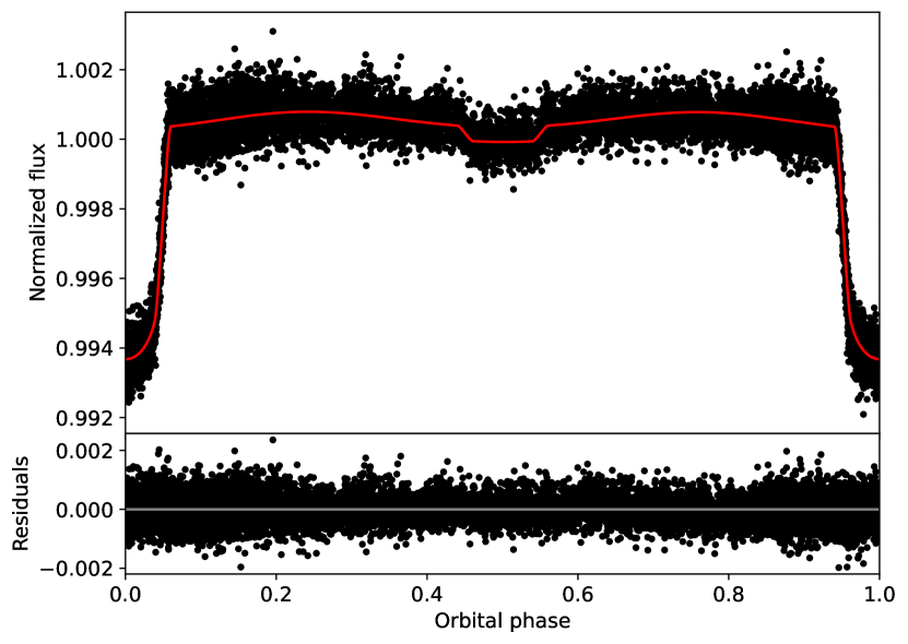
Figure 2: Phase curve fit (top) of the PIPE data (black) shown with TLCM’s median solution phase curve model (red). The residuals of the fit are shown in the bottom plot.

Table 3: Results of the phase curve fits of TOI-2109 b, using the three data sets (CHEOPS (DRP), CHEOPS (PIPE) and TESS).

Parameter	CHEOPS (DRP)	CHEOPS (PIPE)	TESS
$T_{0}$ [BJDTDB]	$10049.588137\pm 0.000062$	$10049.588259\pm 0.000052$	$9730.163124\pm 0.000100$
$P$ [d]	$0.67247397\pm 0.00000009$	$0.67247417\pm 0.00000008$	$0.67248057\pm 0.00000890$
$a/R_{\star}$	$2.202\pm 0.018$	$2.208\pm 0.013$	$2.257\pm 0.053$
$R_{\mathrm{p}}/R_{\star}$	$0.08042\pm 0.00085$	$0.08121\pm 0.00071$	$0.07957\pm 0.00080$
$b$	$0.766\pm 0.017$	$0.769\pm 0.014$	$0.745\pm 0.054$
$i$ [∘]	$69.64\pm 0.25$	$69.61\pm 0.19$	$70.71\pm 0.73$
$A_{\mathrm{g}}$	$1.07\pm 1.35$	$1.08\pm 1.35$	$0.97\pm 1.35$
$\varepsilon[^{\circ}]$	$-1.16\pm 68.35$	$0.59\pm 68.46$	$-1.86\pm 68.61$
$q$	$0.0015\pm 0.0001$	$0.0014\pm 0.0001$	$0.0021\pm 0.0002$
$A$	$1.753\pm 0.449$	$1.313\pm 0.315$	$1.883\pm 0.474$
$B$	$0.932\pm 0.187$	$1.166\pm 0.145$	$0.585\pm 0.302$
$RA_{1}$	$-0.0000527\pm 0.0000069$	-	-
$RA_{2}$	$-0.0000564\pm 0.0000069$	-	-
$RA_{3}$	$-0.0000269\pm 0.0000069$	-	-
$RA_{4}$	$-0.0002591\pm 0.0000078$	-	-
$RA_{5}$	$0.0003812\pm 0.0000077$	-	-
$RA_{6}$	$-0.0001243\pm 0.0000076$	-	-

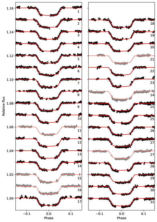
Figure 12: All individual transits from the PIPE data (black) that were fitted using TLCM with the respective transit models (red). The numbers below each transit light curve indicate the number of the corresponding visit, see Table 1. Duplications in visit number refer to the first and second transit in a phase curve observation. If the resulting transit timings were not used in the TTV analysis, they are greyed out.

The mid-transit times obtained from the TLCM fits to the individual transit observations from CHEOPS can be found in Table 7 and for TESS, WASP and the data published in Wong et al. (2021) in Table 8. For these, the transit shape was fixed to the shape determined from the phase curve fits. Even though these fits showed good consistency for the derived parameters, we derived the individual transit timings for both CHEOPS data reductions for comparison. Some of the mid-transit timings were biased due to either missing ingress or egress in the observations, which is why they are filtered out and not used in the following analysis steps. This was determined by visually inspecting the light curves and by comparing the timings retrieved from the DRP and PIPE data – if they agreed well within $1\sigma$, we generally accepted them, except if the timing uncertainties were large ($>30\,$s). All individual transits that were modelled are shown in Fig. 12.

3.3 Discussion

The phase curve fits to the CHEOPS and TESS data show a general agreement between each other for most of the parameters (differences ¡ $1\sigma$ or $2\sigma$ for most of the fitted parameters between the CHEOPS data sets, except for the orbital period at just over $2\sigma$). Larger deviations between CHEOPS and TESS might be explained by their different wavelength ranges, especially for parameters like for the recovered $R_{\mathrm{p}}/R_{\star}$ values. The impact of CHEOPS’ increased precision over TESS can be mainly seen in the recovered transit parameters. Both of them reach comparable precision in the measurements of the phase curve parameters, due to the increased phase coverage and number of full phase curves that are available during one sector with TESS. Assuming only circular orbits is justified by computing the eccentricity damping time scale via (Goldreich & Soter, 1966; Patra et al., 2017):

$$\tau_{e}=\frac{e}{\mathrm{d}e/\mathrm{d}t}=\frac{2\,Q_{\mathrm{p}}}{63\,\pi}\left(\frac{a}{R_{\mathrm{p}}}\right)^{5}\,P,$$ (4)

with $Q_{\mathrm{p}}\sim 10^{6}$ the planetary tidal quality factor of Jupiter, we obtain $\tau_{e}\approx 1.0\,$Myr. Since the system has an age estimate of $1.77^{+0.88}_{-0.68}\,$Gyr, any primordial eccentricity should essentially be reduced to zero. Nevertheless, a small eccentricity might be induced by the companion (Lee & Peale, 2003; Mardling, 2007, 2010; Laskar et al., 2012), and obtaining a full phase curve observation of this planet with e.g. the Hubble Space Telescope (HST) or the James-Webb Space Telescope (JWST, Gardner et al. 2006) would allow the measurement of even small eccentricities at a high precision, which would have the added benefit of allowing a precise atmospheric characterisation. Finding a small eccentricity would provide strong evidence towards the existence of the companion. For a comparison, see the phase curves obtained with JWST for WASP-121 (Mikal-Evans et al., 2023), a star that is relatively similar to TOI-2109, also in magnitude. Such a phase curve should allow very precise characterisation of the orbital characteristics. In particular, the close proximity of this hot Jupiter to its host star and its high equilibrium temperature, in combination with the short orbital period make it a relatively cheap and interesting target to observe. Apart from just determining the atmospheric composition, signs of an escaping atmosphere could be searched for (see e.g. Dos Santos et al. 2023).

Converting the limb darkening parameters back from $A$ and $B$ (for the values see Table 9) to the standard quadratic limb darkening parameters yields $u_{1,\mathrm{DRP}}=0.28\pm 0.17$ and $u_{2,\mathrm{DRP}}=-0.40\pm 0.17$, $u_{1,\mathrm{PIPE}}=0.28\pm 0.12$ and $u_{2,\mathrm{PIPE}}=-0.07\pm 0.12$, and $u_{1,\mathrm{TESS}}=0.28\pm 0.20$ and $u_{2,\mathrm{TESS}}=-0.63\pm 0.20$. The two solutions coming from the CHEOPS data reductions are in good agreement with each other. However, in all cases, we retrieve negative values for the $u_{2}$ component. This and the difference of these limb darkening parameters to the theoretical ones from Claret (2021), which are $u_{1,\mathrm{PHX}}=0.48$ and $u_{2,\mathrm{PHX}}=0.20$ for the stellar atmosphere models from PHOENIX (Husser et al., 2013), and $u_{1,\mathrm{ATL}}=0.31$ and $u_{1,\mathrm{ATL}}=0.31$ for those of ATLAS (Kurucz, 1970) might be explained by the fast stellar rotation, leading to a deformation of the star, and hence to gravity darkening. This should impact the obtained limb-darkening parameters. Nevertheless, the obtained mid-transit timings should be relatively unaffected by this. Comparing our retrieved limb darkening parameters from the TESS data, we find that they agree with the results of Wong et al. (2021) in terms of the resulting radial intensity profile again within $2\sigma$, except for the cross-over point and the outermost range, where we only find a $3\sigma$ agreement.

4 Tidal orbital decay

To search for signs of orbital decay in the measured mid-transit timings from the individual fits to the observed transits, we make use of the standard three models – a linear model describing a constant and circular orbit, a quadratic orbital decay model describing the decreasing orbital period, and a sinusoidal model that represents the effect of apsidal precession on the mid-transit timings (see e.g. Patra et al. 2017; Harre et al. 2023).

The model for the mid-transit times of the constant, circular orbit is given in the following:

$$t_{\mathrm{tra}}(N)=T_{0}+N\,P,$$ (5)

where $N$ is the individual transit number or epoch, $T_{0}$ is the reference timing, and $P$ is the orbital period.

The quadratic orbital decay model describes a change in the orbital period of the planet and is given by:

$$t_{\mathrm{tra}}(N)=T_{0}+N\,P+\frac{1}{2}\,\frac{\mathrm{d}P}{\mathrm{d}N}\,N^{2},$$ (6)

where the decay rate is introduced into the timing model as $\frac{\mathrm{d}P}{\mathrm{d}N}$. This can be converted to the period derivative $\dot{P}$ via:

$$\dot{P}=\frac{\mathrm{d}P}{\mathrm{d}t}=\frac{1}{P}\frac{\mathrm{d}P}{\mathrm{d}N}.$$ (7)

This value can subsequently be plugged into the formulation of Goldreich & Soter (1966) to obtain $Q^{\prime}_{\star}$:

$$\dot{P}=\frac{f\pi}{Q^{\prime}_{\star}}\frac{M_{\mathrm{p}}}{M_{\star}}\left(\frac{R_{\star}}{a}\right)^{5},$$ (8)

with the tidal factor $f=-\frac{27}{2}$, $M_{\mathrm{p}}$ and $M_{\star}$ the planetary and stellar masses, respectively, $R_{\star}$ the stellar radius and $a$ the semi-major axis of the planetary orbit. The given tidal factor is only valid in the case where the planetary orbital period $P$ is shorter than the stellar rotation period $P_{\star}$. For other configurations, $f$ also depends on the true orbital obliquity $\psi$ of the planet, as is shown in Table 2 of Harre et al. (2023). For TOI-2109 b we choose the nominal value, although its fast rotation will likely reduce the effect of the tidal decay, depending on which of the rotation periods that Wong et al. (2021) found in the photometry data is the true one.

The sinusoidal model assumes a slightly eccentric orbit, leading to an apsidal precession motion of the planetary orbit. Using the formulations of Giménez & Bastero (1995), we get:

$$t_{\mathrm{tra}}(N)=T_{0}+N\,P_{\mathrm{s}}-\frac{e\,P_{\mathrm{a}}}{\pi}\,\cos\omega(N),$$ (9)

where $P_{\mathrm{s}}$ is the sidereal period, $P_{\mathrm{a}}$ is the anomalistic period, and $\omega$ is the argument of pericenter. The sidereal and anomalistic period are related via:

$$P_{\mathrm{s}}=P_{\mathrm{a}}\left(1-\frac{1}{2\pi}\frac{\mathrm{d}\omega}{\mathrm{d}N}\right).$$ (10)

The argument of pericenter is linearly related to the transit number, and hence with time, via the following equation:

$$\omega(N)=\omega_{0}+\frac{\mathrm{d}\omega}{\mathrm{d}N}N,$$ (11)

with $\omega_{0}$ the value of the argument of pericenter at the reference time $T_{0}$.

From these fits, using a Markov-chain Monte Carlo algorithm via emcee (Foreman-Mackey et al., 2013), we find no significant orbital decay, nor apsidal precession, and that a linear ephemeris fits the measured mid-transit timings best (see Table 4). Nevertheless, assuming tidal orbital decay to be occuring at the measured rate, and converting the decay rate into the period derivative, we obtain $\dot{P}_{\mathrm{PIPE}}=(-1.32\pm 1.63)$ ms yr^-1 and $\dot{P}_{\mathrm{DRP}}=(-1.10\pm 1.69)$ ms yr^-1. This leads to $95\%$ confidence lower limits of $Q^{\prime}_{\star,\mathrm{PIPE}}>1.6\times 10^{7}$ ($Q^{\prime}_{\star,\mathrm{DRP}}>1.7\times 10^{7}$), and for the decay timescale $\tau=\frac{P}{|\dot{P}|}$, to $\tau_{\mathrm{PIPE}}>12.7$ Myr ($\tau_{\mathrm{DRP}}>13.1$ Myr).

Table 4: Priors and median results of our orbital decay fits for the DRP and PIPE data sets.

Model	Parameter	Prior	CHEOPS (DRP)	CHEOPS (PIPE)
Circular orbit	$T_{0}$ [BJDTDB]	$\mathcal{U}(0,11000)$	$8984.389096\pm 0.000081$	$8984.389120\pm 0.000075$
	$P$ [d]	$\mathcal{U}(0.6,0.75)$	$0.67247425\pm 0.00000007$	$0.67247424\pm 0.00000007$
Orbital decay	$T_{0}$ [BJDTDB]	$\mathcal{U}(0,11000)$	$8984.389120\pm 0.000089$	$8984.389143\pm 0.000080$
	$P$ [d]	$\mathcal{U}(0.6,0.75)$	$0.67247424\pm 0.00000007$	$0.67247423\pm 0.00000007$
	$\mathrm{d}P/\mathrm{d}N$	$\mathcal{U}(-10^{-7},10^{-7})$	$(-2.33\pm 3.57)\times 10^{-11}$	$(-2.80\pm 3.46)\times 10^{-11}$
Apsidal precession	$T_{0}$ [BJDTDB]	$\mathcal{U}(0,11000)$	$8984.389132\pm 0.005254$	$8984.389092\pm 0.005443$
	$P$ [d]	$\mathcal{U}(0.6,0.75)$	$0.67247431\pm 0.00000070$	$0.67247429\pm 0.00000070$
	$\mathrm{d}\omega/\mathrm{d}N$ [rad$/$orbit]	$\mathcal{U}(-0.003,0.003)$	$(0.02\pm 7.04)\times 10^{-4}$	$(0.00\pm 6.51)\times 10^{-4}$
	$e$	$\mathcal{U}(0.0,0.1)$	$0.01619\pm 0.02926$	$0.01896\pm 0.02971$
	$\omega_{0}$ [rad]	$\mathcal{U}(0,2\pi)$	$3.162\pm 1.678$	$3.165\pm 1.633$

Even though this target is one of the best candidates for orbital decay in theory, and the early WASP timing that we obtained gives us a long observation baseline, we only measure a decay rate that is in agreement with a constant orbital period. Comparing with the predictions from Wong et al. (2021) that are in the range of $\sim 10$ – $740\,$ms yr^-1 for the orbital decay rate, we can clearly rule out the upper end of these predictions. This implies that there is another effect which makes the tidal processes less efficient. One possible explanation could be the fast stellar rotation ($v\sin i=(81.2\pm 1.6)$ km s^-1). Even if it is greater ($P_{\mathrm{rot}}/\sin i_{\star}\approx 1.0\,$d, see Wong et al. 2021) than the orbital period of the hot Jupiter, it could still have a negative effect on the efficiency of angular momentum transfer from the planet to the star. The presence of a close-by companion could also affect this. Still, our measured decay rate gives us a constraint on the lower limit of the $Q^{\prime}_{\star}$ value of TOI-2109 that is not too far off from the predicted $Q^{\prime}_{\star}$ values for F-stars of e.g. Ogilvie & Lin (2007); Lanza et al. (2011) that are in the range from $10^{5}$ to $10^{7}$. We also investigated the impact of atmospheric mass loss on the decay rate of the orbit of the hot Jupiter due to its tight orbit. Taking the measurement of the mass loss rate of KELT-9 b of $\dot{M}\sim 10^{12.8\pm 0.3}$ g s^-1 (Wyttenbach et al., 2020) as a first estimate, we find that we would still need two to three orders of magnitude more mass loss for it to balance a decay rate of just $\dot{P}\sim-1$ ms yr^-1, which is unlikely.

One further complication are the apparent sinusoidal TTVs that we observed. Correcting the mid-transit timings for the best fitting super-period of about $117\,$d that we found by fitting the sinusoidal model to the data in Section 5, we find tentative evidence for orbital decay at a rate of $\dot{P}=(-5.56\pm 1.62)\,$ms yr^-1 at $3\sigma$. This would correspond to $95\%$ confidence lower limits of $Q^{\prime}_{\star}>8.4\times 10^{6}$ and $\tau>6.6\,$Myr. We note that this result is sensitive to the applied parameters, because, using the second best fitting super-period of about $88\,$d, the result is less significant with a decreased rate of $\dot{P}=(-3.53\pm 1.63)\,$ms yr^-1 at $2\sigma$. This would lead to lower limits of $Q^{\prime}_{\star}>1.1\times 10^{7}$ and $\tau>8.6\,$Myr at $95\%$ confidence.

Furthermore, the gravitational interactions between the two planets, should the second planet exist, might also have an impact on the orbital decay of the hot Jupiter. In addition to that, should this excite a slight eccentricity in the orbit of TOI-2109 b, it would also introduce apsidal precession. Disentangling the two effects is only possible with very long baselines or very precise mid-occultation timings, which we were not able to obtain with sufficient precision for this task from neither CHEOPS nor TESS. In the future, if a significant orbital decay or apsidal precession signature will be detected from continued monitoring with e.g. CHEOPS, JWST should be able to provide the necessary precision with a few occultation observations. These would also be relatively cheap to obtain due to their short duration, and could give us information about the atmosphere.

However, as shown in Harre & Smith (2023), a distant massive planetary companion would also influence the measured mid-transit timings due to the introduction of a light-time effect. Astrometric observations of Gaia’s (Gaia Collaboration et al., 2016) fourth data release will be able to detect such companions, if they are in the right mass and distance range.

5 An outer companion?

Upon closer inspection of the derived CHEOPS mid-transit times, we noticed a sinusoidal variation that is only significant in these data due to the high precision of the CHEOPS photometry. The first thing we did was to create a Lomb-Scargle (LS) periodogram (Zechmeister & Kürster, 2009) of the transit timings to find possible periods, see Fig. 3. For both, the DRP and PIPE reductions, we obtained multiple peaks of similar powers.

The next step was fitting a simple sinusoidal model to the CHEOPS timings to obtain more information about this sinusoidal variation. We employed the following model (see e.g. Lithwick et al. 2012; Ofir et al. 2018) and optimized it using emcee:

$$t_{\mathrm{tra}}(N)=T_{0}+N\,P+A\,\cos\left(\frac{2\pi}{P_{\mathrm{sup}}}\,(N\,P-T_{\mathrm{sup}})\right),$$ (12)

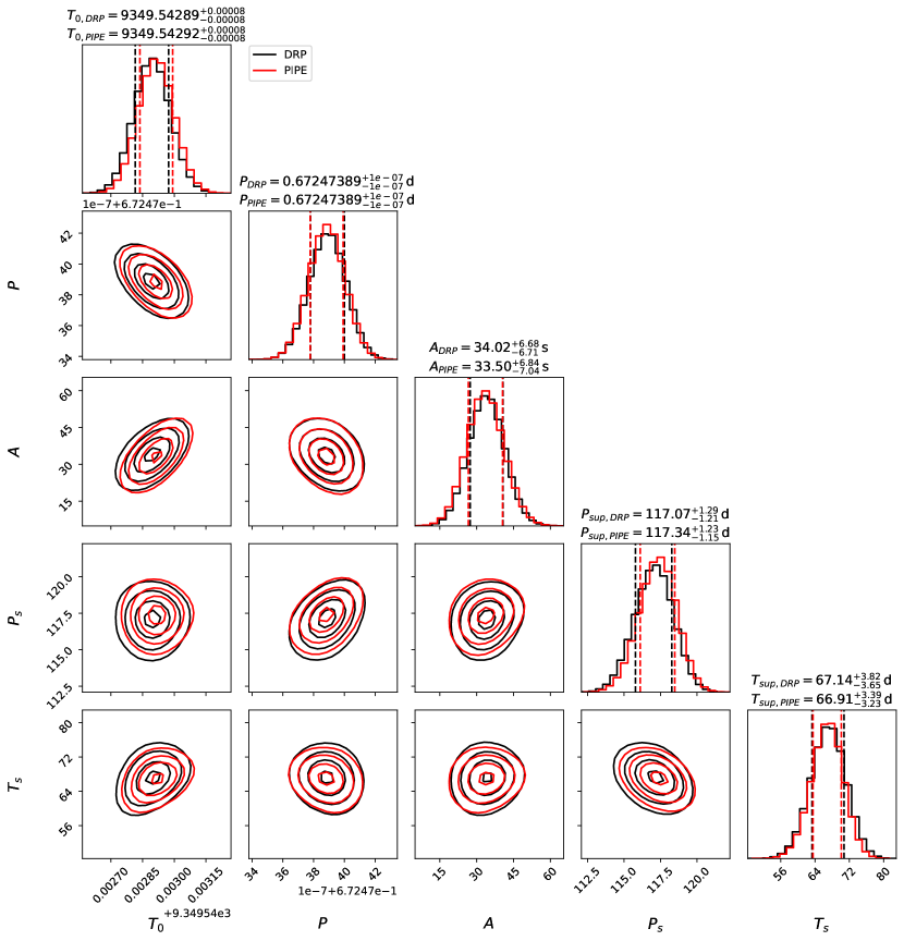
Figure 13: Final corner plot of the fit of the simple sine model (Eq. 12) to the mid-transit timings, measured with CHEOPS using the DRP and PIPE reductions. The dashed lines indicate the $1\sigma$ errors around the median value. The contours show the $0.5\sigma$, $1\sigma$, $1.5\sigma$ and $2\sigma$ levels. $T_{0}$ is given in BJD${}_{\mathrm{TDB}}-2450000$.

where $A$ is the amplitude of the TTVs, $P_{\mathrm{sup}}$ is the super-period and $T_{\mathrm{sup}}$ the super-epoch. To differentiate between the different periods of similar power in the LS periodogram, and to find the best fitting one, we employed multiple MCMC optimisations of our simple TTV model, trying to find the period that leads to the highest log-probability. From this, we determined the parameters of each high-power peak, and sampled them individually for inter-comparison in a further MCMC optimisation (100 walkers, 10000 steps with 1000 steps of burn in). We ensured convergence by checking that the number of steps was at least 50 times the autocorrelation time of all our parameters. We find that $P_{\mathrm{sup}}\approx 117\,$d leads to the lowest BIC value, which is only slightly better ($\Delta\mathrm{BIC}=0.16$) than $P_{\mathrm{sup}}\approx 88\,$d. Both are, however, better than a simple linear model for the mid-transit timings by $\Delta\mathrm{BIC}=4.0$, giving us positive evidence for the apparent TTVs. The final models are shown in Fig. 4 and the respective corner plot in Fig. 13 for both data sets, showing the good agreement between the two data reductions. This, and the agreement of the orbital decay analysis between them prove the consistency of the derived mid-transit timings. Due to this fact, we use, going forward, only the retrieved PIPE timings because the roll-angle effect does not need to be accounted for, which should make the fits to the full data set and the individual timings more reliable.

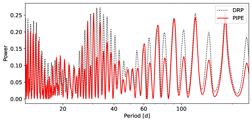
Figure 3: LS periodogram of the transit timing variations measured with CHEOPS, for the DRP and PIPE data reductions.

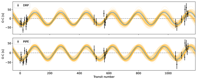
Figure 4: Timing variation plots of the DRP (top) and PIPE (bottom) reductions, showing the lowest BIC models for both data sets. The blue lines show the median solutions, with the thin orange lines showing random samples drawn from the posterior distribution. The dashed gray lines indicate the best linear models.

Due to the relatively high mass of the HJ ($5.02\pm 0.75\,$M_J, see Wong et al. 2021), and amplitude and period of the apparent TTVs, the companion, if present must be relatively close by (Agol et al., 2005). Since we do not find additional transits in the photometric data that is available, we argue that planet c has to orbit outside of the orbit of the HJ. Making use of the Transit Least Squares algorithm (Hippke & Heller, 2019) for the search of additional transits in the residuals of our phase curve fits, we do not find any significant signals. We searched for orbital periods in the range between $1.0\,$d and $15.0\,$d, with the default settings for the search parameters, and the stellar parameters from Wong et al. (2021). Moreover, we also searched for additional transit signals using the Détection Spécialisée de Transits (DST) algorithm (Cabrera et al., 2012), but we did not find any significant evidence of additional planets here either.

The relatively high impact parameter of planet b means that, if planet c is coplanar with planet b, and orbits further out, it will almost certainly not transit the star. In fact, the orbital distance to obtain $b=1.0$, would be $a=5.148\,$R_⊙ or $P=1.125\,$d. In theory, wide ranges of orbital periods and planet masses are possible. Especially the low precision of the RVs due to the fast stellar rotation is a major drawback in this regard, as it is almost impossible to gain any more information about the system, except for planet b, leaving only the observed TTVs as a source of information for the possible companion.

As a first estimate of planet mass and orbital period of the possible outer companion, we use Eq. 33 from Agol et al. (2005). This equation describes the relation between planet masses and TTV amplitude for two planets in MMR, in the case that the more massive planet is transiting. From this, we find masses in the range from 6 to 30 Earth masses for the outer companion, with orbital periods between 1 and 5 days (i.e. MMRs ranging from 3:2 to 7:1).

5.1 Chaotic and regular orbits

Due to the suspected close proximity of the planet candidate, we first explore regular regions in the mass-period space using REBOUND (Rein & Liu, 2012) and its MEGNO (Mean Exponential Growth of Nearby Orbits, Cincotta & Simó 2000) implementation. MEGNO is a chaos indicator for examining the dynamics of planetary systems.

The setup that we have used for the chaos analysis is comprised of a 100 by 100 grid of orbital periods and planetary masses of the outer companion. For each of these grid points, we calculate the MEGNO value. For the setup of the system, we used the parameters given in Wong et al. (2021). Making use of the “WHFast” integrator (Rein & Tamayo, 2015), we integrated the system for more than 270.000 orbits of the inner planet. Both, circular and eccentric systems were probed for completeness. The result for circular orbits is shown in Fig. 5, and for various eccentricities in Appendix D.

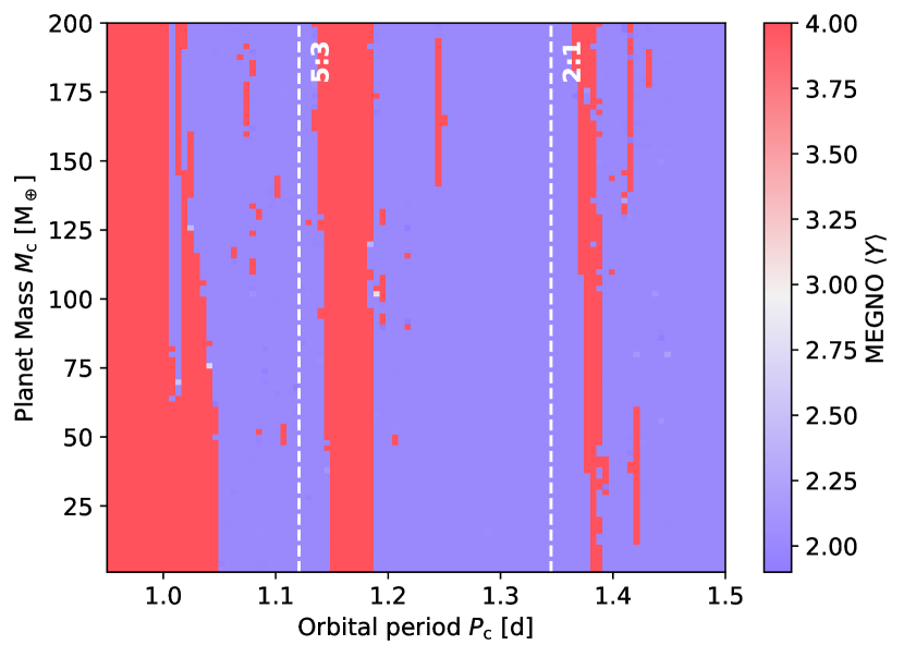
Figure 5: Mass-period MEGNO diagram showing regular and chaotic system configurations for circular orbits of both planets. MEGNO numbers around 2 indicating a regular system (blue), and numbers around 4 indicating a chaotic system (red). The specific mean-motion resonances that are within this period range are indicated as vertical dashed lines.

Probing orbital periods of the outer companion from 0.9 to 1.5 days, and planet masses ranging from 1 to 200 Earth masses, we find that there are a few chaotic areas, especially for very close orbits with $P_{\mathrm{c}}<1.0\,$d. This chaotic area extends up to about $1.05\,$d for low $M_{\mathrm{c}}$ values. There is another chaotic region between about $1.15\,$d and $1.19\,$d for this system. A further, but narrow, chaotic area is present at $P_{\mathrm{c}}\approx 1.39\,$d, with a few more chaotic regions being between these areas. These are, however, mostly small and don’t show the same structure over all examined planetary masses. Beyond orbital periods of $1.5\,$d, there are no significant chaotic areas in the $M_{\mathrm{c}}$ – $P_{\mathrm{c}}$ space for circular orbits of the two planets.

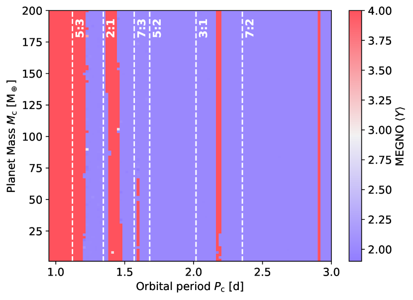
Figure 15: MEGNO plot of TOI-2109 for eccentric orbits of both planets with $e_{\mathrm{b}}=0.03$ and $e_{\mathrm{c}}=0.05$, computed for $270\,000$ orbits of the inner planet.

In the case of eccentric orbits, we find that the innermost regular region gets pushed outwards due to the orbits coming closer together at one point. Depending on the eccentricities used in the simulations, the closest regular area might only be in a narrow area around $1.5\,$d or even farther out (see Fig. 15 – 19).

5.2 TRADES TTV modelling

To model the apparent TTVs in more detail, we employed TRADES (TRAnsits and Dynamics of Exoplanetary Systems) (Borsato et al., 2014, 2019). TRADES is a publicly available N-body code to model the dynamics of exoplanet systems via TTVs and RVs. There are several approaches to obtain the final dynamical solution of the examined system, with us choosing the standard MCMC approach. In two cases, strictly circular or eccentric orbits, we fit for the masses of both planets ($M_{\mathrm{b}}$, $M_{\mathrm{c}}$), the orbital periods ($P_{\mathrm{b}}$, $P_{\mathrm{c}}$) and their mean anomalies ($MA_{\mathrm{b}}$, $MA_{\mathrm{c}}$). This gives us six free parameters for the circular case. In the case of eccentric orbits, we additionally fit for the eccentricities ($e_{\mathrm{b}}$, $e_{\mathrm{c}}$) and their arguments of pericenter ($\omega_{\mathrm{b}}$, $\omega_{\mathrm{c}}$) via $\sqrt{e_{\mathrm{b,c}}}\sin\omega_{\mathrm{b,c}}$ and $\sqrt{e_{\mathrm{b,c}}}\cos\omega_{\mathrm{b,c}}$, giving us a total of ten free parameters. The prior intervals and starting values are given in Table 11. The orbital inclination $i$ was fixed to the angle determined by Wong et al. (2021) for both planets, assuming they share the same orbital plane. Due to the scarcity of information that we expect to be able to extract from the available data, we fixed the longitude of the ascending node to $\Omega=180^{\circ}$ for both planets to reduce the size of the parameter space.

Table 5: Priors used in the setup files for the analysis with TRADES. The values give the starting value and the intervals give the allowed range of the parameters.

Parameter	Planet b	Planet c
$M$ [M${}_{\mathrm{J}}]$	5.02 [4.0, 6.0]	0.2 [0.001, 2.0]
$P$ [d]	0.672474 [0.668, 0.674]	1.9 [0.8, 5.0]
$e$	0.04 [0.0, 0.15]	0.05 [0.0, 0.35]
$\omega$ [∘]	90.0 [0.0, 360.0]	90.0 [0.0, 360.0]
$MA$ [∘]	45.0 [0.0, 360.0]	0.0 [0.0, 360.0]

Making use of the pre-optimisation that TRADES offers via PyDE (Parviainen, 2016), with a population size of 128, generation size of $60\,000$, and a difference amplification factor and cross-over probability of 0.5, we use this initial optimisation as input for emcee. The latter is run for at least $200\,000$ steps, using 128 walkers.

We explored circular and eccentric orbits. In every case, the RVs are also used in the optimisation. Besides these, we explored a few possible MMRs, namely 2:1, 3:1, 5:2, 5:3, 7:2 and 7:3 (ratio of outer to inner period). In these cases, we only allowed a narrow window around the respective resonant orbital period of planet c. All were examined in the cases of circular and eccentric orbits, giving us a total of 12 additional strictly MMR cases. The 3:2 resonance was not probed due to the instability of this close orbital configuration ($P_{\mathrm{c}}\approx 1.0\,$d), as indicated in Fig. 5.

The posterior distributions of the TRADES runs featuring the various MMRs are shown in Fig. 6 and 7, featuring circular and eccentric orbits, respectively.

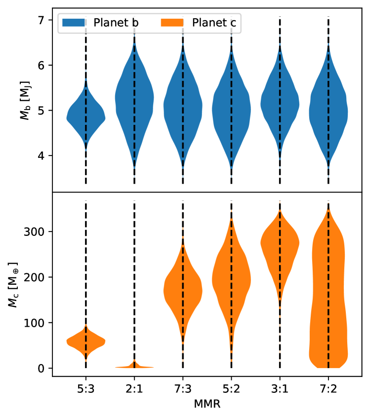
Figure 6: Violin plot of the posterior distributions of the masses of planets ‘b’ (top, blue) and ‘c’ (bottom, orange) derived from the PIPE data in the cases of the MMRs and circular orbits with TRADES.

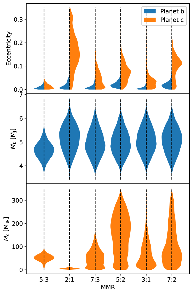
Figure 7: Violin plot of the posterior distributions of the masses and eccentricities from the PIPE data in the cases of the MMRs and eccentric orbits, derived with TRADES.

Comparing the $\chi^{2}$ values of the final results using their maximum-a-posterior (MAP) values, we find the best fit for the 5:3 resonance and eccentric orbits with $\chi^{2}=68.4$, to the available transit timings from CHEOPS and TESS, and the RVs. Even though this specific setup delivers the best fit, the orbit of planet c with these parameters would likely lead to a chaotic system, with it being on the very edge between regular (“stable”) and chaotic (“unstable”). We note that while chaos is linked to instability, regular systems might become unstable after some time. This is owed to the close orbits of the planets in this MMR. The orbital period of $P_{\mathrm{c}}=(1.1398\pm 0.0017)\,$d (with $P_{\mathrm{5:3}}=1.121\,$d being the exact resonance period), and eccentricities of $e_{\mathrm{b}}=0.02$ and $e_{\mathrm{c}}=0.03$, lead to the orbits coming close to each other, so that they may disrupt their orbits. For the purpose of examining the stability of this configuration, we employed $N$-body simulations with REBOUND. First, we tested the stability of the MAP solution by simulating the system for $10^{6}$ yr, which remained stable for this period. Secondly, we checked the stability of $1,000$ randomly drawn samples of the posterior for 100,000 orbits of the inner planet ($\sim 2,000$ yr), and only found $3.5\%$ of them to become unstable within this time. The resulting TTV plot of our fit is shown in Fig. 8. The other runs lead mostly to $\chi^{2}=73-88$, with the 7:2 resonance for circular orbits leading to the worst fits with $\chi^{2}\approx 93$. Checking the stability of these solution for at least $10^{6}$ yr, we find that the MAP values lead to stable orbits for each configuration. Randomly drawing 1,000 samples from each posterior, we find that only six of the resonant configurations have unstable solutions in this sample (including the already mentioned 5:3 MMR in the eccentric case). For the circular 2:1 MMR case, we find that 2 out of 1000 samples become unstable within a time period of 100,000 orbits of the inner planet, the eccentric 2:1 MMR case leads to 281 unstable configurations. For the eccentric cases, the 5:2 MMR leads to 15, the 7:2 MMR to 1, and the 7:3 MMR to 23 unstable solutions. The remaining configurations remain stable over this time frame.

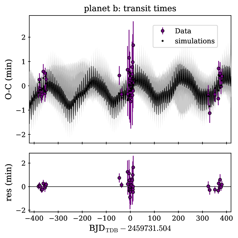
Figure 8: TRADES TTV plot of the best overall fit result, showing a 5:3 MMR and slightly eccentric orbits. Top: Fit to the transit timing measurements of TOI-2109 b, including the final model and random samples from the MCMC analysis. Bottom: Residuals of the fit.

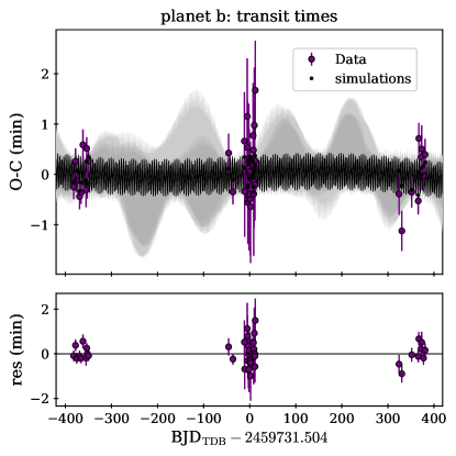
Figure 20: TRADES TTV plot of the general circular orbit fit. Top: Fit to the transit timing measurements of TOI-2109 b, including the final MAP model and random samples from the MCMC analysis. Bottom: Residuals of the fit.

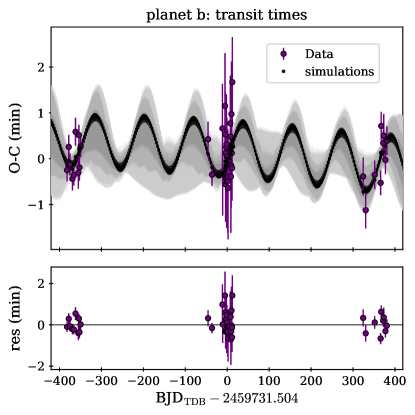
Figure 21: TRADES TTV plot of the general eccentric orbit fit. Top: Fit to the transit timing measurements of TOI-2109 b, including the final MAP model and random samples from the MCMC analysis. Bottom: Residuals of the fit.

In the general runs (for the posteriors see Fig. 9 and 10), without tight constraints on the orbital period of planet c, we obtain the best result in terms of $\chi^{2}$ value for eccentric orbits, resulting in $\chi^{2}=75.1$. The final orbital period of planet c in this case is actually very close to a 4:1 MMR with $P_{c}=2.677\,$d, where the exact MMR period would be $P_{\mathrm{4:1}}=2.688\,$d. The TTV plot is shown in Fig. 21. It reproduces the super-period of about $\sim 117\,$d that we also found using the simple sinusoidal model (see Fig. 4). The model allowing circular orbits fits worse by $\Delta\chi^{2}\approx 3.5$, with a final period of the outer companion close to the 7:3 MMR. The respective TTV plot is shown in Fig. 20.

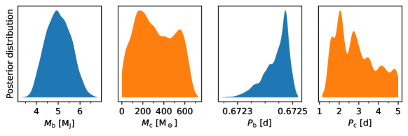
Figure 9: Posterior distributions of the masses and periods for the general run ($P_{\mathrm{c}}$ not constrained to be near a certain MMR) for circular orbits, derived with TRADES. The results for planet b are indicated in blue and for c in orange.

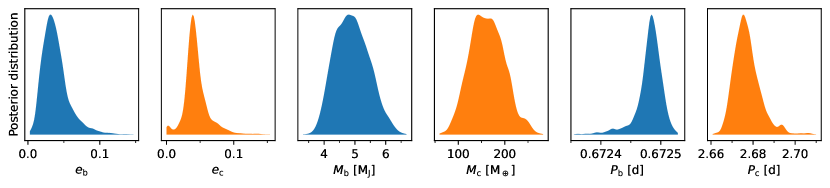
Figure 10: Posterior distributions of the eccentricities, masses and periods for the general run ($P_{\mathrm{c}}$ not constrained to be near a certain MMR) for eccentric orbits, derived with TRADES. The results for planet b are indicated in blue and for c in orange.

5.3 PyTTV analysis

We carry out a set of photodynamical analyses modelling the CHEOPS PIPE transit timings, TESS photometry, and the TRES and FIES radial velocities jointly using PyTTV (Korth et al., 2023). The code models the three types of observables (transit photometry, radial velocity measurements, and transit centre time estimates) simultaneously using REBOUND (Rein & Liu, 2012; Rein & Spiegel, 2015; Tamayo et al., 2020) for dynamical integration and PyTransit (Parviainen, 2015; Parviainen & Korth, 2020; Parviainen, 2020) for transit modelling, and provides posterior densities for the model parameters estimated using MCMC sampling in a standard Bayesian parameter estimation framework. We employ PyTTV in addition to TRADES to make sure that our results are broadly consistent due to the weak constraints that we have of the system.

The model parameters and their priors are listed in Table 6. All the planet parameters except for the log₁₀ mass and radius ratio are defined at a reference time, $t_{\mathrm{ref}}=2459378.46$. We set uniform priors on the log masses of the two planets, with ranges designed to help optimisation but not to constrain the posteriors. We set a loosely informative prior on the inner planet’s radius ratio based on the Wong et al. (2021) estimate, and the outer planet’s radius ratio is given a dummy normal prior since the data will not be able to constrain it. We set a normal prior on the inner planet’s transit center and a uniform prior on the outer planet’s mean anomaly (the planets are parameterized differently since the hot Jupiter transits and the other does not). We do not constrain the mutual inclinations of the two planets. Instead, we set an informative prior on the inner planet’s impact parameter based on the Wong et al. (2021) estimate of $0.7481\pm 0.0073$, and we set an uniform prior on the outer planet impact parameter. The lower limit of the outer planet’s impact parameter prior is justified by the fact that the planet does not transit, and the upper limit was checked no to constrain the posterior after the MCMC sampling. Finally, we set additional zero-centered half-normal priors on the eccentricities, $\mathcal{N}$(0.0, 0.023). These priors allow for eccentric orbits but bias against high eccentricities.

The analysis begins with a global optimisation using the differential evolution method (Storn & Price, 1997; Price et al., 2005) implemented in PyTransit (Parviainen, 2015). The optimiser starts with a population of parameter vectors drawn from the model prior, and clumps the population close to the global posterior mode. After the optimisation, we use the clumped parameter vector population to initialise the emcee sampler (Foreman-Mackey et al., 2013), which we then use for MCMC sampling to obtain a sample from the parameter posterior.

We repeat the analysis for the 5:3, 2:1, 7:3, 5:2, 3:1, and 7:2 period commensurability scenarios. For each scenario, we set the outer planet period prior to $\mathcal{N}(r\times 0.67247414,0.1)$, where $r$ is the period ratio for the scenario.

We present the posterior distributions for the planet masses, orbital inclinations, and orbital eccentricities from the PyTTV analysis in Fig. 11. The Bayesian Information Criterion (BIC) favours the 3:1 period commensurability scenario, which also has a relatively small difference in the orbital inclinations. Looking at the individual likelihoods from the photometry, transit centres, and RVs, the 3:1 scenario is mainly favoured by the improved fit of the RV measurements. Indeed, the photometry and transit centre likelihood distributions corresponding to the posterior parameter distributions largely overlap, as do the ones for the RV data for all the other scenarios than 3:1.

Table 6: PyTTV model parameters and priors.

Description	Units	Prior
Stellar parameters
Stellar mass	[$M_{\odot}$]	$\mathcal{N}(1.447,0.077)$
Stellar radius	[$R_{\odot}$]	$\mathcal{N}(1.698,0.060)$
Limb darkening q${}_{1}^{a}$	[-]	$\mathcal{U}(0,1)$
Limb darkening q${}_{2}^{a}$	[-]	$\mathcal{U}(0,1)$
Planet b parameters
log10 mass	[$\log_{10}\,M_{\odot}$]	$\mathcal{U}(-2.8,-2.1)$
Radius ratio	[$R_{\star}$]	$\mathcal{N}(0.08,0.001)$
Transit centre	[BJD]	$\mathcal{N}(2459378.46,0.02)$
Orbital period	[d]	$\mathcal{N}(0.67247414,0.005)$
Impact parameter	[$R_{\star}$]	$\mathcal{N}(0.75,0.01)$
$\sqrt{e}\cos\omega$	[-]	$\mathcal{U}(-0.25,0.25)$
$\sqrt{e}\sin\omega$	[-]	$\mathcal{U}(-0.25,0.25)$
$\Omega$	[rad]	$\mathcal{N}(\pi,0.0001)$
Planet c parameters
log10 mass	[$\log_{10}\,M_{\odot}$]	$\mathcal{U}(-5.2,-3.0)$
Radius ratio	[$R_{\star}$]	$\mathcal{N}(0.05,0.0001)$
Mean anomaly at $T_{\mathrm{ref}}$	[rad]	$\mathcal{U}(0,2\pi)$
Orbital period	[d]	Depends on the scenario
Impact parameter	[$R_{\star}$]	$\mathcal{U}(1.0,3.0)$
$\sqrt{e}\cos\omega$	[-]	$\mathcal{U}(-0.25,0.25)$
$\sqrt{e}\sin\omega$	[-]	$\mathcal{U}(-0.25,0.25)$
$\Omega$	[rad]	$\mathcal{N}(\pi,0.0001)$
RV parameters
Linear trend	[m/s/d]	$\mathcal{N}(0,1.0)$
Systemic velocity 1	[m/s]	$\mathcal{N}(-25855,200)$
Systemic velocity 2	[m/s]	$\mathcal{N}(-25416,200)$
log10 jitter 1	[$\log_{10}$ m/s]	$\mathcal{N}(-1,0.1)$
log10 jitter 2	[$\log_{10}$ m/s]	$\mathcal{N}(-1,0.1)$
Additional priors
Both eccentricities		$\mathcal{N}(0.0,0.023)$

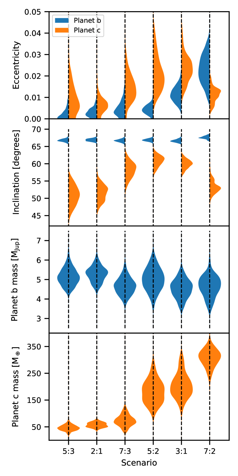
Figure 11: Posterior densities for the planet masses, orbital inclinations, and orbital eccentricities obtained from the PyTTV analysis for the six considered period commensurability scenarios.

5.4 Discussion of the TTV analysis

Since we did not find additional transits in the available photometric data and due to the close proximity of the hot Jupiter to its host star, we establish that the companion has to be orbiting outside of the orbit of TOI-2109 b, should it exist. Furthermore, if planet c’s orbit is aligned with that of planet b, it would have to orbit with $P_{\mathrm{c}}<1.125\,$d to be transiting (which would roughly correspond to a 5:3 MMR), indicating a longer orbital period than this lower limit, which all of our tested cases correspond to. In theory, there are regular orbital solutions interior to the hot Jupiter, however the probability for the inner planet to not transit would be relatively small, requiring a large misalignment with a nearly polar orbit with the orbital plane having to be aligned almost perfectly perpendicular to our line of sight.

Unfortunately, the fast rotation of the host star hinders the precise measurement of RVs due to the inherent line broadening that this characteristic leads to. This means that it is unlikely that the close companion candidate will be confirmed using this method, even if many observations are taken with high-precision instruments. A major drawback is also the loose constraint on TOI-2109 b’s mass. The dynamical model would benefit from a reduced parameter space to better constrain the other fitted parameters. A possible solution for the characterisation of this system could be to obtain at least two phase curve observations with JWST (see e.g., Mikal-Evans et al. 2023; Bell et al. 2024). This would give us six precise timing measurements (four occultation timings and two transit timings) that, if spread out sufficiently over the phase of a sinusoid, have the potential to massively constrain the parameter space for the dynamical analysis of this system.

The results of our TRADES TTV analysis reveal many possible orbital configurations that could, due to the loose contraints that we only have of the system, result in the apparent TTVs that have been observed. Some of the examined cases show poor convergence, which could not always be ensured owing to either the constraints that we enforced in the cases where we examined specific MMRs, or stochastic variations in the pre-optimisation procedure. Checking the stability of the circular orbit MMR solutions, we find that all of them seem to lead to regular systems and are stable for at least 1 Myr using the MAP solutions. However, the 5:3 MMR case leads to a final system configuration and orbital period ($P_{\mathrm{c}}=1.139\,$d) that is close to the chaotic area, but on the verge of the regular regime, as can be seen in Fig. 5. Nevertheless, we find the MAP solution to be stable for at least 1 Myr using $N$-body simulations, all of the 1,000 randomly drawn samples of the posterior to be stable for 100,000 orbits of the hot Jupiter. The overall best-fitting result was obtained from the 5:3 MMR case, where we allowed non-zero eccentricities. According to REBOUND simulations using the final MAP parameters from TRADES, we obtain stable orbits for at least 1 Myr using $N$-body simulations. Even the grand majority of 1,000 randomly drawn samples of the posterior are stable for 100,000 orbits of the inner planet. However, the regular area is relatively tight within the mean-longitude – period space, using the MEGNO indicator. Nevertheless, this was our overall best-fitting result.

The best-fitting result that we obtained from our general circular TRADES fit (see Fig. 20) shows a relatively high-frequency modulation of the TTVs, with some of the chains reproducing the trend that is seen in Fig. 8. Our result allowing eccentric orbits in the general case (see Fig. 21) is close to a 4:1 MMR and also reproduces the TTV super-period of $\sim 117\,$d that we found to be the best fit using the simple sinusoidal model (see. Fig. 4 and Fig. 13). Even if we cannot solve the system with the data that is available, this provides a good agreement between the two approaches and is evidence that the apparent sinusoidal TTVs are real. In theory, TTVs of this amplitude could be caused by starspot crossing events (Ioannidis et al., 2016), but this seems quite unlikely in this case due to the star being an F-type star, and the very low probability of this effect to occur consistently over 3 observing seasons. In addition, we did not find signs of starspot crossings in the transits that we captured with CHEOPS.

Investigating the stability of the remaining cases that we examined, we find that the individual MAP solutions are all stable for 1 Myr, as tested with REBOUND, and as has been seen for the circular orbits. Randomly drawing samples from the posterior and testing their stability also finds that most solutions are stable for 100,000 orbits of the hot Jupiter (see Section 5.2. For the general runs we observe that in both cases, circular and eccentric orbits, all tested solutions lead to stable systems over the examined time frames.

Regarding the PyTTV analysis, we find the 3:1 MMR to lead to the best fit, mainly due to the RV data. This means that the RV data may provide some evidence of planet c, though this evidence remains tentative at best, due to the large RV uncertainties, the TTVs have the highest impact in the fitting process. Before comparison of these results from those of TRADES, we first of all have to note the different approaches that were chosen for the two codes. While we are using the same data sets in both cases, we fit for more parameters using PyTTV due to its faster and more flexible approach, where especially the inclusion of the orbital inclination might have an impact on the results. Here, we also only focused on the specific MMRs in cases where we allow non-zero eccentricities. Comparing the results (Fig. 7 and Fig. 11), we can see the effect that PyTTVs photodynamical model has on the final fits by inspecting the final eccentricities. PyTTVs achieves better convergence due to it being able to better break the mass-eccentricity degeneracies that can be seen for the TRADES equivalents of the runs. Lower eccentricities should lead to more stable systems, especially for such tight systems, while in the case of TRADES, we find greater possible eccentricities for planet c, especially in the 2:1, 5:2 and 7:2 MMRs cases. Which can explain the differences in the posterior mass ranges. Other than this, the posteriors mostly agree with each other and show similar trends, remaining difference can be explained by the inclinations of planet c in the PyTTV runs.

6 Conclusions

By examining newly obtained CHEOPS photometry of the TOI-2109 system, we discovered sinusoidal transit-timing variations (TTVs) while searching for signs of tidal orbital decay, the latter of which we find tentative evidence for when correcting the mid-transit timings using a simple sinusoidal model that describes the TTVs best. Being unable to discover additional transits in the available photometry, we conclude that the candidate planet c must orbit outside of TOI-2109 b’s orbit with a period greater than $P_{\mathrm{c}}\approx 1.13\,$d owing to the high impact parameter and the orbital inclination of planet b, assuming co-planar orbits. Probing the apparent TTVs using a simple sine model, we found that two super-periods ($P_{\mathrm{sup}}\approx 88\,$d and $P_{\mathrm{sup}}\approx 117\,$d) fit the observations best, when compared to a simple linear model, giving us positive evidence ($\Delta\mathrm{BIC}=4$) for the authenticity of the TTVs.

Applying the N-body code TRADES (Borsato et al., 2014, 2019) to our data set (for other examples see e.g., Malavolta et al. 2017; Nespral et al. 2017; Borsato et al. 2019; Nascimbeni et al. 2023; Borsato et al. 2024), we find that the best-fitting solution corresponds to a 5:3 mean-motion resonance (MMR) with $P_{\mathrm{c}}=(1.1398\pm 0.0017)\,$d and slight eccentricities. This solution is stable for at least 1 Myr, according to our $N$-body simulations using REBOUND. From general, non-strictly MMR fits, we find orbital periods of the outer candidate companion of about $P_{\mathrm{c}}\approx 1.57\,$d (close to a 7:3 MMR) in the circular case and $P_{\mathrm{c}}\approx 2.67\,$d (close to a 4:1 MMR) in the eccentric case. The free eccentric fit solutions are compatible with the best-fitting super-period that we found during our investigation of the TTVs with the simple sinusoidal model. And even some of the chains of the circular general fit reproduce our best-fitting model of the 5:3 MMR with eccentricities. In addition to TTV analysis with TRADES, we also made use of PyTTV (Korth et al., 2023). While we do not find the same preference of the 5:3 MMR, we find a slight preference of the 3:1 MMR and a similar posterior distributions between the codes in general. Differences can between the two can be explained by the different approach that was chosen in the modelling, with more parameters being included in PyTTV that were fixed in the TRADES analysis to achieve faster convergence. Owing to the low amplitude of the TTVs and the quality of the radial velocity measurements caused by the fast rotation of the stellar host, we cannot fully confirm the new planetary candidate yet, or which of the models is preferred overall. More precise timing measurements are necessary in this regard. Continued monitoring with CHEOPS would be a possible solution and would also support the search of orbital decay, since the TESS observations have not been precise enough in terms of the precision of the retrieved mid-transit timings.

Besides CHEOPS, HST or JWST observations of this system would not only allow atmospheric characterisation of this short period, ultra-hot Jupiter, but also give us the opportunity to obtain very precise timing measurements, even if only a few were obtained. Spread out over the phase of the possible sinusoids, six precise timings from two phase curve observations (four occultation timings and two transit timings) could massively constrain the parameter space, and should enable us to fully confirm this planet and better determine its characteristics. Due to the close orbit, these observations wouldn’t be very expensive in terms of observation time.

Confirming the existence of the planet candidate would add TOI-2109 to the rare class of hot Jupiters with close companions and would make it only the second of these systems to host an outer companion, like it is present in the WASP-47 system (Becker et al., 2015; Almenara et al., 2016; Neveu-VanMalle et al., 2016; Vanderburg et al., 2017; Nascimbeni et al., 2023).

Appendix A Individual transit plots

Appendix B Retrieved mid-transit timings

Table 7: Mid-transit times of TOI-2109 b, retrieved from the CHEOPS DRP and PIPE data reductions. Potentially biased timings were filtered out. Transit epochs given relative to our timing from the phase curve fits. Times given in BJD${}_{\mathrm{TDB}}-2450000$.

Epoch	TimeDRP	ErrorDRP [d]	TimePIPE	ErrorPIPE [d]
-1041	9349.542546	0.000232	9349.542445	0.000169
-1035	9353.577576	0.000211	9353.577643	0.000182
-1031	9356.267243	0.000191	9356.267276	0.000165
-1022	9362.319158	0.000177	9362.319324	0.000177
-1017	9365.681918	0.000173	9365.681752	0.000159
-1011	9369.717019	0.000213	9369.717254	0.000212
-1001	9376.441345	0.000240	9376.441376	0.000241
-999	9377.786845	0.000212	9377.786895	0.000156
-997	9379.131546	0.000213	9379.131353	0.000202
-993	9381.821608	0.000187	9381.821568	0.000166
-541	9685.779757	0.000335	9685.780035	0.000269
-527	9695.194240	0.000254	9695.194138	0.000172
-475	9730.163441	0.000220	9730.163262	0.000181
-471	9732.852594	0.000230	9732.852663	0.000208
-470	9733.525305	0.000203	9733.525374	0.000194
-465	9736.887592	0.000222	9736.887740	0.000206
-456	9742.940224	0.000199	9742.940237	0.000178
9	10055.640153	0.000280	10055.640304	0.000289
18	10061.692214	0.000278	10061.692062	0.000277
50	10083.211849	0.000252	10083.211774	0.000216
71	10097.333665	0.000266	10097.333611	0.000187
73	10098.679387	0.000284	10098.679421	0.000216
80	10103.386211	0.000235	10103.386483	0.000191
82	10104.731772	0.000289	10104.731543	0.000327
88	10108.766204	0.000203	10108.766020	0.000215
93	10112.128585	0.000224	10112.128684	0.000217

Table 8: Mid-transit times of TOI-2109 b, retrieved from the ground-based data published in Wong et al. (2021), WASP and TESS. Transit epochs given relative to our timing from the phase curve fits. Times given in BJD${}_{\mathrm{TDB}}-2450000$. Only a portion of the table is shown to indicate its form and contents. The full table can be retrieved from the CDS.

Epoch	Time	Error [d]	Source
-9166	3885.688618	0.001079	WASP
-1584	8984.387648	0.002520	TESS
-1583	8985.063895	0.002520	TESS
-1582	8985.733954	0.001407	TESS
…	…	…	…

Appendix C Sine fit corner plot

Appendix D Additional MEGNO eccentricity plots

Figure 14: MEGNO plot of the TOI-2109 system for a circular orbit of the hot Jupiter and a slightly eccentric orbit of planet c ($e_{\mathrm{c}}=0.05$), for $270\,000$ orbits of the inner planet.

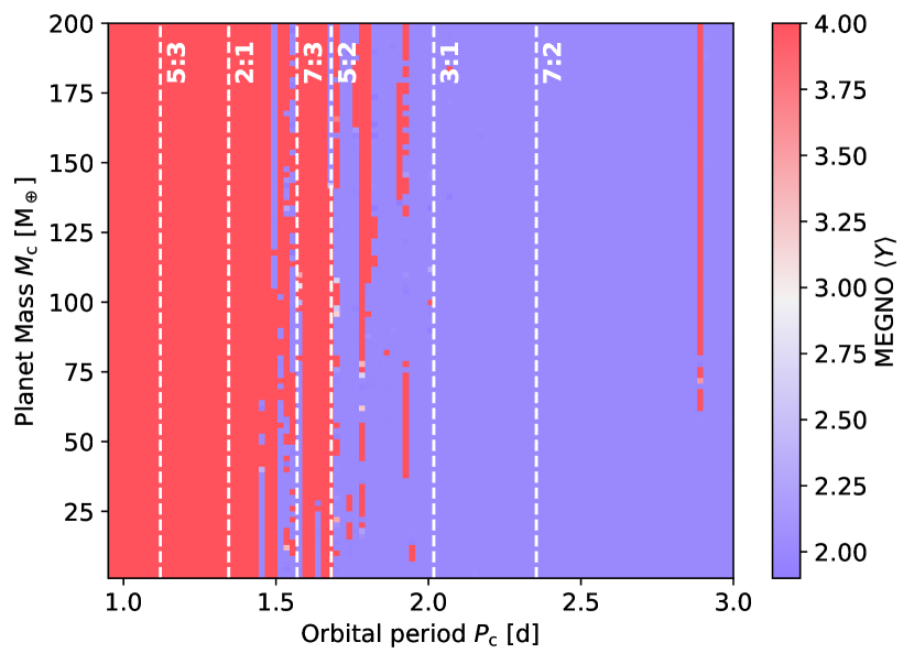
Figure 16: MEGNO plot of the TOI-2109 system for a circular orbit of the hot Jupiter and a moderately eccentric orbit of planet c ($e_{\mathrm{c}}=0.15$), for $270\,000$ orbits of the inner planet.

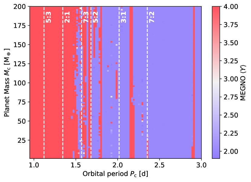
Figure 17: MEGNO plot of TOI-2109 for eccentric orbits of both planets with $e_{\mathrm{b}}=0.03$ and $e_{\mathrm{c}}=0.15$, computed for $270\,000$ orbits of the inner planet.

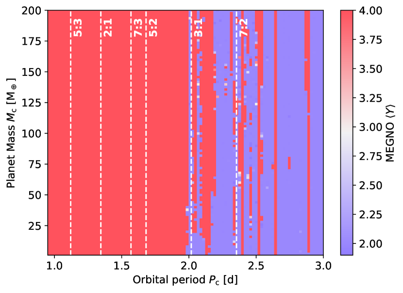
Figure 18: MEGNO plot of the TOI-2109 system for a circular orbit of the hot Jupiter and an eccentric orbit of planet c ($e_{\mathrm{c}}=0.25$), for $270\,000$ orbits of the inner planet.

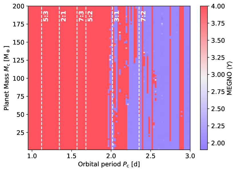
Figure 19: MEGNO plot of TOI-2109 for eccentric orbits of both planets with $e_{\mathrm{b}}=0.03$ and $e_{\mathrm{c}}=0.25$, computed for $270\,000$ orbits of the inner planet.

Appendix E Additional TRADES TTV plots