Nonclassicality and sub-Planck structures of photon subtracted compass states

Abstract

We discuss the nonclassical properties of photon-subtracted compass states (PSCS). Nonclassical behavior is studied using various parameters like the Wigner function, squeezing, and photon statistical parameters like Mandel’s Q-function, second-order correlation function, Agarwal–Tara $A_{3}$ criterion, and photon number distribution. Further analysis is being done to investigate the sub-Planck structures in the Wigner functions of these PSCS. We also show that the photon subtraction causes the loss of sensitivity due to displacement of the states in phase space.

I Introduction

The generation and analysis of nonclassical states of the electromagnetic field have become increasingly significant in quantum optics and quantum information[1, 2] over the past few decades. Coherent state [3] of light exhibits the classical nature, characterized by localized Gaussian wave packets and a photon distribution that follows Poissonian statistics. The manipulation of such coherent states gives rise to various nonclassical states. Microscopically distinct quantum states, when superposed, exhibit properties characteristic of quantum behavior. Cat states [4], compass states [5], and quantum hypercube states [6] are examples of superposition states utilized in cat codes for quantum error correction (QEC). As interest serges to generalize various coherent states [7, 8, 9, 10], the superposition of such generalized coherent states leads to many versions of cat state [11, 12]. Especially compass state [5] which is the superposition of four coherent states, has the important property that its Wigner quasi-probability distribution function has structures that are below the Plank constant for certain parameter values. Many generalizations of compass states[13, 14] as well as their sub-Plank structures have been studied in recent times. It was believed that these structures do not play any physical role but Zurek [15] shows that these structures are very important in determining the sensitivity of the system to decoherence [16] and phase space displacements. Advancements in quantum state engineering in recent decades have made the preparation and study of nonclassical states through operations such as squeezing, displacing states in phase space, photon addition, and photon subtraction, increasingly important. Agarwal and Tara [17] introduced the photon-added coherent state which was later experimentally realized by Zavatta et al [18], who reported the first excitation of the coherent state by homodyne tomography technology. Adding photons to the cat state also changes the state property significantly. The photon-added cat state [19] is experimentally realized by Yi-Ru Chen et al [20]. Subtracting a photon from an even cat state just leads to an odd cat state, and both even and odd cat states are the eigenstate of the $\hat{a}^{2}$ operator[4]. Subsequently, the photon-added compass state is studied by G. Ren et al. [21]. Photon subtraction to the compass state is the eigenstate of $\hat{a}^{4}$ operator, which are just superpositions of cat states. One such photon-subtracted compass state (PSCS) can be created by propagating a coherent state through an amplitude-dispersive medium[22].
Given the recent experimental advancements[23, 18] in generating non-Gaussian radiation fields and the tomographic reconstruction of Wigner functions for quantum states, it is an opportune moment to examine the non-classical properties of photon-subtracted states. In this paper, we want to focus on the study of the nonclassical features of the photon-subtracted compass states. The organization of the paper is as follows. In section II we introduce the photon subtracted compass states (PSCS) and formulate its general form for the convenience of calculation also the generalized version of the state helps us to understand the superposition of two cat states with different amplitudes. Section III discusses the nonclassical properties of the states in terms of the negativity of the Wigner function and other statistical properties like Mandel’s Q-Parameter, second-order correlation function, Agarwal-Tara criterion, photon number distribution and we calculate the squeezing for the states also. In section IV we discuss the sub-Planck structures in the phase space of Wigner quasi-probability distribution function of the states. We also discuss the sensitivity of the states due to the small displacement of the state in the phase space. Concluding remarks are given in section V

II Photon subtracted compass state

Zurek’s compass state is a superposition of four coherent states.

$$\ket{\psi_{0}}=N_{0}\{\ket{\alpha}+\ket{-\alpha}+\ket{i\alpha}+\ket{-i\alpha}\}$$ (1)

Here $\ket{\alpha}$ is the coherent state, and the $N_{0}$ is the normalization constant. When $l$ numbers of photons $(l>0)$ are subtracted from the compass state, the state becomes $\ket{\psi_{l}}=\hat{a}^{l}\ket{\psi_{0}}$. Here $l=1,2,3$. Further photon subtraction ie, $(l=4)$ leads to the same compass state $\ket{\psi_{0}}$ as these states are the eigenstates of $\hat{a}^{4}$.
The general compass state (GCS) can be written as

$$\ket{\psi(\theta,\phi,\chi)}=N\{(\ket{\alpha}+e^{i\theta}\ket{-\alpha})+e^{i\phi}(\ket{\beta}+e^{i\chi}\ket{-\beta})\}\quad\alpha,\beta\in\mathbb{C}$$ (2)

The normalization constant

$$\begin{split}N=\biggl{[}4+2e_{\alpha}^{2}\cos\theta+2e_{\beta}^{2}\cos\chi+2\sqrt{e_{\alpha}e_{\beta}}\biggl{(}e^{\xi\cos{k}}\cos{(\phi+\xi\sin{k})}+e^{-\xi\cos{k}}\cos{(\phi-\theta-\xi\sin{k})}\\ \quad+e^{-\xi\cos{k}}\cos{(\phi+\chi-\xi\sin{k})}+e^{\xi\cos{k}}\cos{(\phi+\chi-\theta+\xi\sin{k})}\Bigr{]}\biggr{)}\biggr{]}^{\frac{1}{2}}\end{split}$$

Where $\alpha^{*}\beta=\xi e^{ik}$ and $e_{\alpha}=e^{-\absolutevalue{\alpha}^{2}}$, and $e_{\beta}=e^{-\absolutevalue{\beta}^{2}}$
By setting $\beta=i\alpha$ and the phases appropriately in Eq. 2 we obtain the compass state $\ket{\psi_{0}}\equiv\ket{\psi(0,0,0)}$ and PSCS $\ket{\psi_{1}}\equiv\ket{\psi(\pi,\frac{\pi}{2},\pi)}$,$\ket{\psi_{2}}\equiv\ket{\psi(0,\pi,0)}$,$\ket{\psi_{3}}\equiv\ket{\psi(\pi,\frac{3\pi}{2},\pi)}$. In the general compass state $\ket{\psi(\theta,\phi,\chi)}$ in Eq. 2, when $\beta\neq i\alpha$, the state $\ket{\psi(\theta,\phi,\chi)}$ is no longer an eigenstate of $\hat{a}^{4}$, Rather it is like the superposition of two cat states of different amplitude.

III Nonclassicality

III.1 Wigner Function

Wigner function [24, 25] corresponds to a state $\hat{\rho}$ is a quasi-probability distribution function in the phase space. The negativity of this Wigner function is a strong indicator of the nonclassicality of the state. In $(x,y)$ phase space, Wigner function is defined for the state $\hat{\rho}$ is

$$W(z)=\frac{2}{\pi^{2}}e^{2\absolutevalue{z}^{2}}\int d^{2}\nu\matrixelement{-\nu}{\hat{\rho}}{\nu}\exp{2(\nu^{*}z-\nu z^{*})}$$ (3)

where $z=x+iy$ and $\ket{\nu}$ is a coherent state. For any pure state $\ket{\psi}$, the density matrix is $\hat{\rho}=\outerproduct{\psi}{\psi}$. Using the general compass state in Eq. 2 the Wigner function is

$$W_{\ket{\psi(\theta,\phi,\chi)}}(z)=\frac{2N^{2}}{\pi}e^{2\absolutevalue{z}^{2}}\Bigl{[}\sqrt{e_{\alpha}}\sum_{i=1}^{2}e^{-\absolutevalue{a_{i}}^{2}}+\sqrt{e_{\beta}}\sum_{j=3}^{4}e^{-\absolutevalue{a_{j}}^{2}}+\sum_{l=1}^{6}m_{l}\Bigr{]}$$ (4)

here $a_{1}=2z+\alpha$,$a_{2}=2z-\alpha$,$a_{3}=2z+\beta$ and $a_{4}=2z-\beta$

$$m_{1} =2e_{\alpha}e^{-\xi_{1}}\cos{(\theta-k_{1})}\quad\text{with }a_{1}a_{2}^{*}=\xi_{1}+ik_{1}$$

$$m_{2} =2\sqrt{e_{\alpha}e_{\beta}}e^{-\xi_{2}}\cos{(\theta-\phi-\chi-k_{2})}\quad\text{with }a_{1}a_{3}^{*}=\xi_{2}+ik_{2}$$

$$m_{3} =2\sqrt{e_{\alpha}e_{\beta}}e^{-\xi_{3}}\cos{(\theta-\phi-k_{3})}\quad\text{with }a_{1}a_{4}^{*}=\xi_{3}+ik_{3}$$

$$m_{4} =2\sqrt{e_{\alpha}e_{\beta}}e^{-\xi_{4}}\cos{(-\phi-\chi-k_{4})}\quad\text{with }a_{2}a_{3}^{*}=\xi_{4}+ik_{4}$$

$$m_{5} =2\sqrt{e_{\alpha}e_{\beta}}e^{-\xi_{5}}\cos{(-\phi-k_{5})}\quad\text{with }a_{2}a_{4}^{*}=\xi_{5}+ik_{5}$$

$$m_{6} =2e_{\beta}e^{-\xi_{6}}\cos{(\chi-k_{6})}\quad\text{with }a_{3}a_{4}^{*}=\xi_{6}+ik_{6}$$

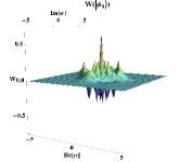
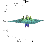
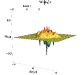
Figure 1: Wigner Function of compass state and PSCS for $\alpha=2$

The first four terms in Eq. 4 correspond to the Gaussian peaks of the four coherent states and the six $m_{l}$ terms are the interference terms. Wigner functions of the compass and PSCS $(\ket{\psi_{l}};l=0,1,2,3)$ are plotted in Fig. 1 for $\alpha=2$. We see that successive photon subtraction from the compass state $\ket{\psi_{0}}$ makes the interference terms flip the signs and change the amplitude alternatively. One way to quantify the effect of photon subtraction and the change in amplitude of the interference terms is to see the negative volume of the Wigner function. Kenfack et al. [26], showed that the amount of negative volume in phase space accounts for the non-classicality of a state. The more negative the volume, the more nonclassical the behavior. The negative volume is calculated using the formula.

$$\delta(\ket{\psi})=\int\int\absolutevalue{W_{\ket{\psi}}(x,y)}dxdy-1$$ (5)

Fig. 2 shows that for our states $\ket{\psi_{l}}$ ($l=0,1,2,3$), the amount of negative volume $\delta(\ket{\psi_{l}})$ is significantly different for different $l$ when $\alpha$ is small. The negative volume for $\ket{\psi_{1}},\ket{\psi_{2}},\ket{\psi_{3}}$ is more than $\ket{\psi_{0}}$. So the photon subtraction causes the increase in the negative volume of the Wigner function. Also, varying the magnitude of $\beta\neq i\alpha$ the amount of negative volume of the Wigner function is changed.

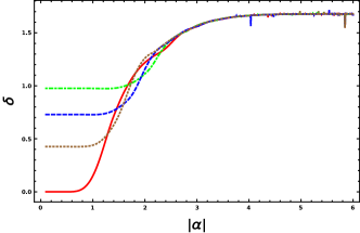
(a) (b)

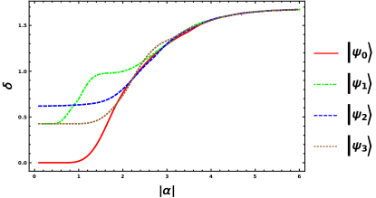
Figure 2: Negative volume ($\delta(\ket{\psi_{l}})$) of the Wigner function of (a) the compass and PSCS (ie, $\beta=i\alpha$) (b) Generalise compass state with $\beta=\frac{i\alpha}{2}$

III.2 Statistical properties

III.2.1 Mandel’s Q-Parameter

Mandel’s Q-parameter is an indicator used to measure how a quantum state’s photon number distribution deviates from the Poissonian distribution, typical of a coherent state. The Q-Parameter defined as [27, 28]

$$Q=\frac{\expectationvalue{\hat{n}^{2}}-\expectationvalue{\hat{n}}^{2}}{\expectationvalue{\hat{n}}}-1$$ (6)

Here $\hat{n}=\hat{a}^{\dagger}\hat{a}$. When the Q-parameter is zero, the state exhibits Poissonian statistics, similar to a coherent state. If the Q-parameter is positive $(Q>0)$, the state demonstrates super-Poissonian statistics, which means there is photon bunching, and the variance in the photon number is higher than that of a coherent state. On the other hand, a negative Q-parameter$(Q<0)$ signifies sub-Poissonian statistics, indicating photon antibunching, where the variance in the photon number is lower than that of a coherent state. This reduction in variance is a hallmark of non-classical light. Using the general cat superposition state the values of the expectation is

$$\begin{split}\expectationvalue{\hat{a}^{{\dagger}m}\hat{a}^{m}}&=N^{2}\biggl{[}2\absolutevalue{\alpha}^{2m}\{1+(-1)^{m}e_{\alpha}^{2}\cos\theta\}+2\absolutevalue{\beta}^{2m}\{1+(-1)^{m}e_{\beta}^{2}\cos\chi\}\\ &\quad+2\xi^{m}\sqrt{e_{\alpha}e_{\beta}}\biggl{(}e^{\xi\cos{k}}\cos{(\phi+km+\xi\sin{k})}+(-1)^{m}e^{-\xi\cos{k}}\cos{(\phi-\theta+km-\xi\sin{k})}\\ &\quad+(-1)^{m}e^{-\xi\cos{k}}\cos{(\phi+\chi+km-\xi\sin{k})}+e^{\xi\cos{k}}\cos{(\phi+\chi-\theta+km+\xi\sin{k})}\Bigr{]}\biggr{)}\biggr{]}\end{split}$$ (7)

so for $m=1$, we calculate the average photon number $\expectationvalue{\hat{n}}=\expectationvalue{\hat{a}^{\dagger}\hat{a}}$ and to find $\expectationvalue{\hat{n}^{2}}$ we note that $\expectationvalue{\hat{n}^{2}}=\expectationvalue{\hat{a}^{{\dagger}2}\hat{a}^{2}}+\expectationvalue{\hat{n}}$ where the first part is obtained by setting $m=2$ in Eq. 7.

Using these two expectation values, we derive the final Q-parameter from Eq. 6. The resulting graph in Fig. 3 shows that the Q parameter of the PSCS oscillates about $Q=0$. For low values of $\alpha$ the photon subtraction makes the states more nonclassical, as the Q-parameter for $\ket{\psi_{1}},\ket{\psi_{2}},$ and $\ket{\psi_{3}}$ is more negative compared to the compass state $\ket{\psi_{0}}$. As $\alpha$ increases, the Q-parameter for all states approaches zero, indicating that they approach classical states with Poissoinian distribution. But in Fig. 3 there are values of $\alpha$ for which the $Q>0$ for the compass state and PSCS but other parameters suggest these states are nonclassical. In these values of $\alpha$, no conclusion can be drawn about the nonclassicality of these states only observing the Q-parameter.

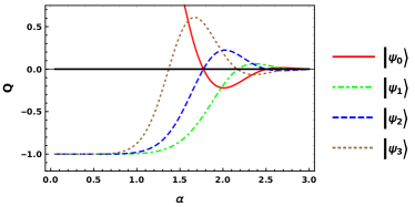
Figure 3: Mandel’s Q-parameter of compass state and PSCS

III.2.2 Second order Correlation function

The Mandel’s Q-parameter cannot confirm a state’s nonclassicality, since a state can be non-classical despite having a positive Q value. The equal time second-order correlation function $g^{2}(0)$ [29] tells about the bunching or anti-bunching property of the state similar to the Q parameter. If $g^{2}(0)=1$, the state exhibits Poissonian photon statistics. When $g^{2}(0)<1$, the state demonstrates photon antibunching, indicative of sub-Poissonian statistics. Conversely, if $g^{2}(0)>1$, the state shows photon bunching, reflecting super-Poissonian statistics.

$$g^{2}(0)=\frac{\expectationvalue{\hat{a}^{{\dagger}2}\hat{a}^{2}}}{\expectationvalue{\hat{a}^{\dagger}\hat{a}}^{2}}$$ (8)

The expectation values are obtained from Eq. 7 by setting $m=1,2$, and the second-order correlation function is calculated. The compass and photon-subtracted compass states have a Q value that oscillates around 0 value. The same oscillatory behavior can be seen in the $g^{2}(0)$ about 1 value but when we zoom in we can see values of $\alpha$ for which $Q>0$ but $g^{2}(0)<1$. So in these values of $\alpha$, the states are nonclassical according to $g^{2}(0)$. However, there are also certain values of $\alpha$ for which $Q>0$ but $g^{2}(0)>1$. So the state is super-Poissionian in those values of $\alpha$. For example, from Fig. 3 and 4 we see that in case of $\ket{\psi_{0}}$ and $\ket{\psi_{3}}$ for $\absolutevalue{\alpha}=1.5$,$Q$ is positive and $g^{2}(0)>1$. This kind of confusion arises when we try to predict the nonclassical/classical nature of these states $\ket{\psi_{l}}$. To resolve the contradiction, another improved version of nonclassicality criteria must be checked for these values of $\alpha$.

Figure 4: Second order Correlation $g^{2}(0)$ for compass and PSCS

III.2.3 Agarwal–Tara Criterion

Agarwal and Tara introduced a moment-based criterion to check for the nonclassicality of a state having no sub-Poisssionion or squeezing [30]. As per the criterion, a state is nonclassical if

$$A_{3}=\frac{\text{det }m^{(3)}}{\text{det }\mu^{(3)}-\text{det }m^{(3)}}<0$$ (9)

where

$$m^{(3)}=\begin{bmatrix}1&m_{1}&m_{2}\\ m_{1}&m_{2}&m_{3}\\ m_{2}&m_{3}&m_{4}\end{bmatrix}\quad\text{and }\quad\mu^{(3)}=\begin{bmatrix}1&\mu_{1}&\mu_{2}\\ \mu_{1}&\mu_{2}&\mu_{3}\\ \mu_{2}&\mu_{3}&\mu_{4}\end{bmatrix}$$

Here $m_{i}=\expectationvalue{\hat{a}^{{\dagger}i}\hat{a}^{i}}$ and $\mu_{j}=\expectationvalue{(\hat{a}^{\dagger}\hat{a})^{j}}$ are the matrix elements.
The $m_{i}$ are calculated from the general expression of Eq. 7 and the $\mu_{j}$ are calculated by expanding $(\hat{a}^{\dagger}\hat{a})^{j}$ in normally ordered form [31]. The result obtained for $A_{3}$ is shown in Fig. 5 which shows the nonclassical behavior for the compass state and photon subtracted compass states. The figure shows that for all values of $\alpha$, $A_{3}$ are negative indicating nonclassicality despite the fact that $Q>0$ and $g^{2}(0)>1$ for a range of values of $\alpha$. According to Agarwal and Tara’s criteria, the compass state and PSCS are nonclassical in nature.

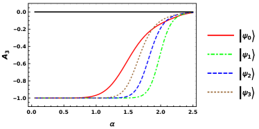
Figure 5: Agarwal,Tara parameter $A_{3}$ vs $\alpha$ for compass and PSCS

III.2.4 Photon number Distribution

The photon number distribution(PND) of a state is a good indicator of nonclassicality. It is the probability of the state to be in a fock state $\ket{n}$. The PND for any state $\hat{\rho}$ is

$$P(n)=Tr[\hat{\rho}\outerproduct{n}{n}]$$ (10)

For GCS $\hat{\rho}=\outerproduct{\psi(\theta,\phi,\chi)}{\psi(\theta,\phi,\chi)}$ the PND is

$$P(n)=N^{2}\frac{1}{\sqrt{n!}}[\alpha^{n}e^{-\frac{\absolutevalue{\alpha}^{2}}{2}}\{1+e^{i\theta}(-1)^{n}\}+e^{i\phi}\beta^{n}e^{-\frac{\absolutevalue{\beta}^{2}}{2}}\{1+e^{i\chi}(-1)^{n}\}]$$ (11)

The variance of the Photon Number Distribution (PND) in photon-subtracted compass states is smaller than that of a Poisson distribution. This finding aligns with the results obtained using the Mandel parameter and the second-order correlation function. In Fig. 6 we see that $P(n)$ for $\ket{\psi_{0}}$ is nonzero at $n=20,24,28...$, that is at an interval of 4. A similar feature appears for PSCS i.e. $\ket{\psi_{1}}$ having nonzero probabilities at $n=19,23,27...,$$\ket{\psi_{2}}$ having nonzero probabilities at $n=18,22,26...,$$\ket{\psi_{3}}$ having nonzero probabilities at $n=17,21,25...,$ , which suggests successive photons are subtracted.

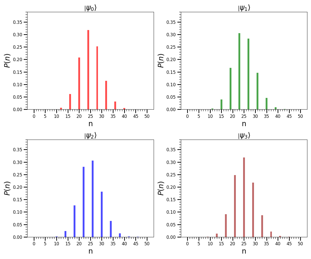
Figure 6: Photon Number Distribution for compass and PSCS for $\alpha=5$

III.3 Squeezing

Squeezing is a well-known non-classical effect which is a phenomenon in which variance in one of the quadrature components becomes less than that in a vacuum state or coherent state. General quadrature operator

$$\hat{X}=\frac{1}{2}(\hat{a}e^{-i\theta^{{}^{\prime}}}+\hat{a}^{\dagger}e^{i\theta^{{}^{\prime}}})\quad\text{and}\quad\hat{Y}=\frac{1}{2i}(\hat{a}e^{-i\theta^{{}^{\prime}}}-\hat{a}^{\dagger}e^{i\theta^{{}^{\prime}}})$$ (12)

The quadrature operators follow the commutation relation $[\hat{X},\hat{Y}]=\frac{i}{2}$, and uncertainty relation $(\triangle\hat{X})^{2}(\triangle\hat{Y})^{2}\geq\frac{1}{16}$. If $(\triangle\hat{X})^{2}<\frac{1}{4}$ or the parameter $S_{X}=4(\triangle\hat{X})^{2}-1\leq 0$ then the $X$ quadrature is squeezed. Similarly if the parameter $S_{Y}=4(\triangle\hat{Y})^{2}-1\leq 0$ then the $Y$ quadrature is squeezed.
The uncertainty in quadrature in terms of boson creation and annihilation operator is

$$(\triangle\hat{X})^{2}=\frac{1}{4}(e^{-2i\theta^{{}^{\prime}}}\expectationvalue{\hat{a}^{2}}+e^{2i\theta^{{}^{\prime}}}\expectationvalue{\hat{a}^{{\dagger}2}}+2\expectationvalue{\hat{a}^{\dagger}\hat{a}}-e^{-2i\theta^{{}^{\prime}}}\expectationvalue{\hat{a}}^{2}-e^{2i\theta^{{}^{\prime}}}\expectationvalue{\hat{a}^{{\dagger}}}^{2}-2\expectationvalue{\hat{a}}\expectationvalue{\hat{a}^{{\dagger}}}+1)$$ (13)

$$(\triangle\hat{Y})^{2}=-\frac{1}{4}(e^{-2i\theta^{{}^{\prime}}}\expectationvalue{\hat{a}^{2}}+e^{2i\theta^{{}^{\prime}}}\expectationvalue{\hat{a}^{{\dagger}2}}-2\expectationvalue{\hat{a}^{\dagger}\hat{a}}-e^{-2i\theta^{{}^{\prime}}}\expectationvalue{\hat{a}}^{2}-e^{2i\theta^{{}^{\prime}}}\expectationvalue{\hat{a}^{{\dagger}}}^{2}+2\expectationvalue{\hat{a}}\expectationvalue{\hat{a}^{{\dagger}}}-1)$$ (14)

The expectation values in terms of compass and PSCS is

$$\begin{split}\expectationvalue{\hat{a}^{2}}=N^{2}[2\alpha^{2}e^{-2\absolutevalue{\alpha}^{2}}(\cos{\theta}-\cos{\chi})-2i\alpha^{2}e^{-\absolutevalue{\alpha}^{2}}\{\sin{(\phi+\absolutevalue{\alpha}^{2})}+\sin{(\phi+\chi-\theta+\absolutevalue{\alpha}^{2})}\\ +\sin{(\phi-\theta-\absolutevalue{\alpha}^{2})}+\sin{(\phi+\chi-\absolutevalue{\alpha}^{2})}\}]\end{split}$$ (15)

$$\begin{split}\expectationvalue{\hat{a}}=N^{2}[2\alpha e^{-2\absolutevalue{\alpha}^{2}}(-i\sin{\theta}+\sin{\chi})+\alpha e^{(i-1)\absolutevalue{\alpha}^{2}}\{ie^{i\phi}-ie^{i(\phi+\chi-\theta)}-e^{i(\theta-\phi)}+e^{-i(\phi+\chi)}\}\\ +\alpha e^{(-i-1)\absolutevalue{\alpha}^{2}}\{e^{-i\phi}-e^{-i(\phi+\chi-\theta)}+ie^{-i(\theta-\phi)}-ie^{i(\phi+\chi)}\}]\end{split}$$ (16)

using the fact that $\expectationvalue{\hat{a}^{\dagger}}=\expectationvalue{\hat{a}}^{*}=0$ ,$\expectationvalue{\hat{a}^{{\dagger}2}}=\expectationvalue{\hat{a}^{2}}^{*}=0$ and the expectation value of $\expectationvalue{\hat{n}}=\expectationvalue{\hat{a}^{\dagger}\hat{a}}$ from Eq. 7 by setting $\beta=i\alpha$; the expectation of the quadrature uncertainty is calculated. From Eq. 13 and 14 we can see that the uncertainties in both the quadrature is equal ie. $S_{X}=S_{Y}$, also from Fig. 7 it is seen that both $S_{X}$ and $S_{Y}$ are positive for all four states, which indicates no squeezing occurs. The figure also indicates that the increase in uncertainty in the quadrature for low values of $\alpha$ is due to the photon subtraction to the compass state. For higher values of $\alpha$, the difference in uncertainties in all the states diminishes.

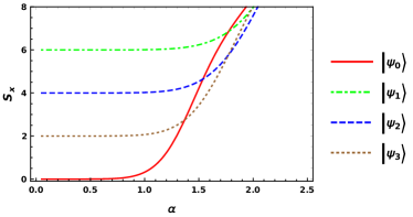
Figure 7: Squeezing of $X$ and $Y$ quadrature for compass and PSCS

We also checked if the GCS has Hong–Mandel type higher-order squeezing. A state is said to have Hong–Mandel type squeezing [32, 33, 34] if

$$S(l)=\frac{\expectationvalue{(\Delta X)^{l}}-(\frac{1}{2})_{\frac{l}{2}}}{(\frac{1}{2})_{\frac{l}{2}}}<0$$ (17)

Here where $(x)_{l}$ is the conventional Pochhammer symbol. The expectation of nth order moment of $X$ quadrature is

$$\expectationvalue{(\Delta X)^{l}}=\sum_{r=0}^{l}\sum_{i=0}^{\frac{r}{2}}\sum_{k=0}^{r-2i}(-1)^{r}\frac{1}{2^{\frac{l}{2}}}(2i-1)!\binom{2i}{k}\binom{l}{r}\binom{r}{2i}\expectationvalue{a^{\dagger}+a}^{l-r}\expectationvalue{(a^{\dagger})^{k}a^{r-2i-k}}$$ (18)

Here we see that the term $\expectationvalue{a^{\dagger}+a}^{l-r}=0$ as $\expectationvalue{\hat{a}^{\dagger}}=\expectationvalue{\hat{a}}^{*}=0$. Thus $S(l)=-1$. Thus the compass and PSCS exhibit Hong–Mandel type of higher order squeezing.

III.3.1 Quadrature Distribution

The quadrature ket in terms of the Fock basis is

$$\bra{x}=\pi^{-1/4}\bra{0}exp{(-\frac{x^{2}}{2}+\sqrt{2}x\hat{a}-\frac{\hat{a}^{2}}{2})}$$ (19)

hence the Coherent state in terms of the quadrature variable is

$$\innerproduct{x}{\alpha}=\pi^{-1/4}exp{(-\frac{x^{2}}{2}+\sqrt{2}x\alpha-\frac{\alpha^{2}}{2}-\frac{\absolutevalue{\alpha}^{2}}{2})}$$ (20)

for GCS, the quadrature distribution is defined by

$$\textbf{P}(x) =\absolutevalue{\innerproduct{x}{\psi(\theta,\phi,\chi)}}^{2}$$ (21)

$$\innerproduct{x}{\psi(\theta,\phi,\chi)} =\pi^{-1/4}e^{-\frac{x^{2}}{2}}\bigl{\{}e^{-\frac{\alpha^{2}}{2}-\frac{\absolutevalue{\alpha}^{2}}{2}}(e^{\sqrt{2}x\alpha}+e^{i\theta}e^{-\sqrt{2}x\alpha})+e^{i\phi}e^{-\frac{\beta^{2}}{2}-\frac{\absolutevalue{\beta}^{2}}{2}}(e^{\sqrt{2}x\beta}+e^{i\chi}e^{-\sqrt{2}x\beta})\bigr{\}}$$ (22)

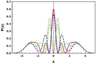
(a) (b)

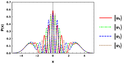
Figure 8: Quadrature distribution of (a) the compass and PSCS for $\alpha=2$ and (b) GCS for $\alpha=2$ and $\beta=2i\alpha$

From Fig. 8(a) we see that the quadrature distribution of the compass and PSCS have an oscillating behavior. However, the width of the distribution doesn’t change for the PSCS. This suggests that the photon subtraction doesn’t affect the width of the quadrature distribution and we expect no squeezing of quadrature to occur. This is indeed what we observe in the previous calculation of squeezing parameters $S_{x}$ and $S_{y}$ to be positive. For GCS the quadrature distribution is shown in Fig. 8(b) for $\beta=2i\alpha$. Here also the quadrature distribution is highly oscillatory and the width of the quadrature distributions doesn’t change significantly suggesting no squeezing.

IV Subplank Structure

The product of uncertainties in quadrature variables is bounded by a minimum value of $\Delta x\Delta p=1$, often referred to as the Planck action in phase space. This minimum value is equivalent to $\frac{\hbar}{2}$ when considering position and momentum in appropriate units.
Wigner Function in Eq. 4, the first four terms are the Gaussian lobe due to the four coherent states, and the $m_{2}$ to $m_{5}$ terms are the mutual interference terms of the adjacent Gaussian peaks. Finally, the $m_{1}+m_{6}$ is the chessboard-like pattern in the middle of the four Gaussian peaks, the area of such small boxes gets smaller by increasing the amplitude of $\alpha$. If $\alpha=x_{0}$ or $\alpha=ip_{o}$ then for the photon subtracted compass states

$$(m_{1}+m_{6}) \sim e^{-4\left(x^{2}+y^{2}\right)}\{\cos(4x_{0}x)+\cos(4x_{0}y)\}\quad\text{for }\alpha=x_{0}$$

$$(m_{1}+m_{6}) \sim e^{-4\left(x^{2}+y^{2}\right)}\{\cos(4p_{0}x)+\cos(4p_{0}y)\}\quad\text{for }\alpha=ip_{0}$$

Thus the area of the boxes is proportional to $\frac{1}{x_{0}^{2}}$ (for $\alpha=x_{0}$) or $\frac{1}{p_{0}^{2}}$ (for $\alpha=ip_{0}$) so for large $x_{0}$ or $p_{o}\gg 1$ the structure is below plank scale.
The area of the smallest tiles remains consistent across all generalized photon-subtracted compass states. This consistency arises because the contributions from $(m_{1}+m_{6})$ in the Wigner function of Eq. 4 are identical in magnitude but differ by a negative sign after each photon subtraction. Consequently, as shown in Fig. 9, photon subtraction results in a transformation of the tiles, where the regions of positive and negative values are rearranged. This rearrangement reflects the impact of photon subtraction, altering the distribution of these regions within the Wigner function.

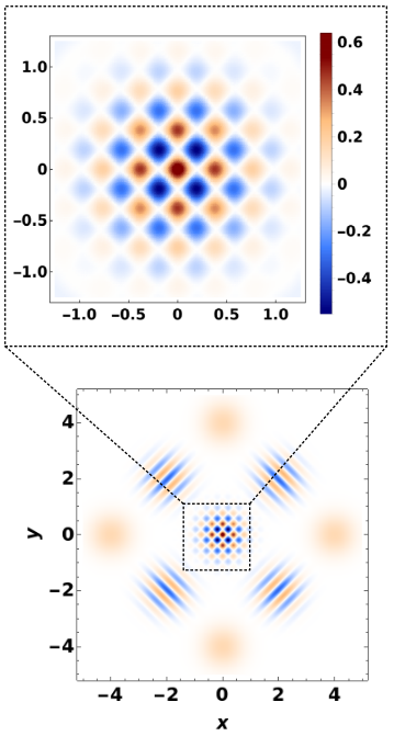
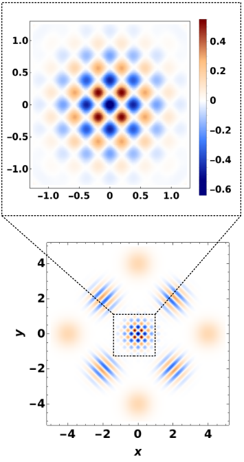
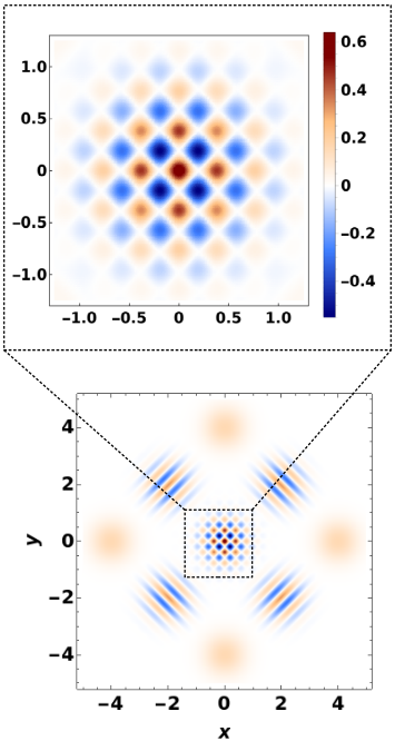
(a) (b) (c) (d)

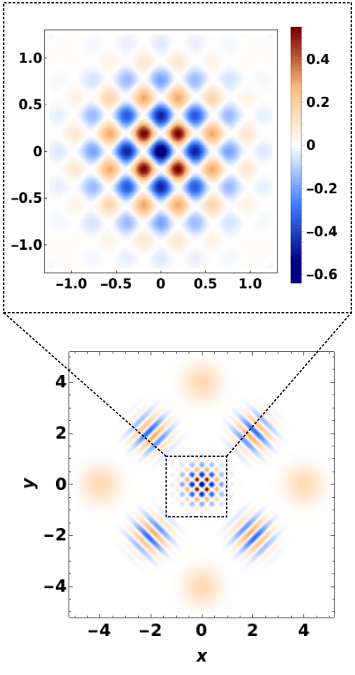
Figure 9: Density plot of the Wigner function and the zoomed version of the chessboard-like pattern in the middle for (a) compass state $\ket{\psi_{0}}$ and (b) PSCS $\ket{\psi_{1}}$, (c) PSCS $\ket{\psi_{2}}$, (d) PSCS $\ket{\psi_{3}}$ for $\alpha=4$.

IV.1 Sensitivity to displacement

For any arbitrary state $\hat{\rho}$ the sensitivity of the state due to displacement is defined by the overlap of the displaced state with the original state. The sensitivity is thus

$$F_{\hat{\rho}}(\delta)=tr[\hat{\rho}\hat{D}(\delta)\hat{\rho}\hat{D}^{\dagger}(\delta)]$$ (23)

and for any pure state $\hat{\rho}=\outerproduct{\psi}{\psi}$ the sensitivity is $F_{\hat{\rho}}(\delta)=\absolutevalue{\expectationvalue{\hat{D}(\delta)}{\psi}}^{2}$. Hear $\delta=\delta_{x}+i\delta_{p}$ is the amount of arbitrary small displacement in the phase space. The $\hat{D}(\delta)$ is displacement operator.

$$\hat{D}(\delta)=exp(\delta\hat{a}^{\dagger}-\delta^{*}\hat{a})$$ (24)

The overlap for our generalized compass state in Eq. 2

$$\begin{split}F_{\ket{\psi(\theta,\phi,\chi)}}(\delta)&=\absolutevalue{\expectationvalue{\hat{D}(\delta)}{\psi(\theta,\phi,\chi)}}^{2}\\ &=\absolutevalue{\{N^{2}\bra{\alpha}+e^{-i\theta}\bra{-\alpha}+e^{-i\phi}\bra{-\beta}+e^{-i(\phi+\chi)}\bra{-\alpha}\}\hat{D}(\delta)\{\ket{\alpha}+e^{i\theta}\ket{i\alpha}+e^{i\phi}\ket{i\beta}+e^{i(\phi+\chi)}\ket{i\beta}\}}^{2}\end{split}$$ (25)

Now this $\expectationvalue{\hat{D}(\delta)}{\psi(\theta,\phi,\chi)}$ contains 16 terms and the main contributing part to the sensitivity due to the sub-Planck structure is

$$\sum_{\begin{subarray}{c}\sigma_{l}=\pm 1\\ \alpha_{j}=\alpha,\beta\end{subarray}}\expectationvalue{\hat{D}(\delta)}{\sigma_{l}\alpha_{j}}=\sum_{\begin{subarray}{c}\sigma_{l}=\pm 1\\ \alpha_{j}=\alpha,\beta\end{subarray}}exp\Bigl{\{}i\sigma_{l}Im[\delta\alpha_{j}^{*}]-\frac{\absolutevalue{\alpha_{j}}^{2}}{2}-\frac{\absolutevalue{\sigma_{l}\alpha_{j}+\delta}^{2}}{2}+\alpha_{j}^{*}(\alpha_{j}+\sigma_{l}\delta)\Bigr{\}}$$ (26)

Now for the symmetric compass state ie, $\beta=i\alpha$ and its photon subtracted states the overlap is approximately the same for all four states. The compass and PSCS show sensitivity due to displacement in arbitrary direction as shown in Fig. 10(a).
But for the nonsymmetric case i.e. $\beta\neq i\alpha$ also the sensitivity doesn’t depend on the relative phase $(\theta,\phi,\chi)$, and the sensitivity due to displacement is in an arbitrary direction. The shape of the Fig. 10(b) changes as per the amplitude of the $\alpha$ and $\beta$.

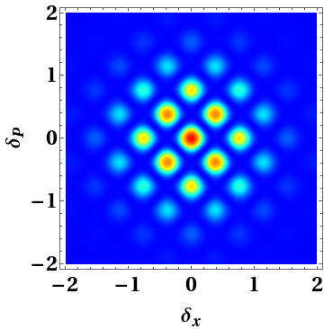
(a) (b)

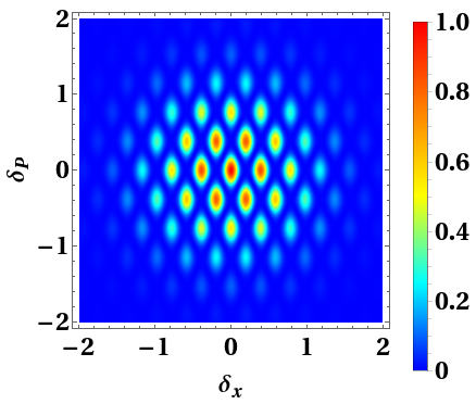
Figure 10: Sensitivity of the (a)compass state and PSCS ($\beta=i\alpha$) for $\alpha=4$ and (b) GCS for $\beta=2i\alpha$

V Conclusion

In this work, we discussed the properties of the compass state and the effect of photon subtraction on it. We generalize the states as the superposition of the two cat states. When the amplitude of the two cat states are equal ie, $\beta=i\alpha$, then setting the phase parameters, we get the compass and PSCS, and for $\beta\neq i\alpha$ we get the two superposed cat states.
We have shown that the nonclassicality is increased due to photon subtraction to the compass state and to check the degree of nonclassicality we have calculated various nonclassicality parameters. The negativity in the Wigner function exhibited by the compass and PSCS is quantified by the negative volume measure. The negativity of the Mandels Q parameter and the photon number distribution shows the sub-Poissionia nature of the fields, and the second-order correlation function $g^{2}(0)<1$ shows the antibunching of the radiation fields. Agarwal–Tara $A_{3}$ parameter confirms the nonclassicality for all values of $\alpha$. We have shown that none of the states show squeezing by calculating the quadrature distribution and the degree of squeezing but the states show Hong–Mandel type higher-order squeezing.
The compass and PSCS states are essentially the superposition of four coherent states, thus showing the sub-Planck structure in the Wigner distribution. We have shown that due to the photon subtraction, the area of the chessboard-like tiles remains the same for all the PSCS and compass states but the signs of the Wigner functions changed due to the successive photon subtraction. We also showed that the sensitivity of the states due to the displacement of the state in the phase space is very small. The sensitivity of the PSCS is the same as the compass state ie, the states are sensitive to all directions. For $\beta=2i\alpha$ the sensitivity structure changes and it is more sensitive to one direction than the other.

VI Acknowledgment

Amit Das would like to acknowledge UGC JRF, Govt. of India for financial support.

References

- Kok [2010] P. Kok, Entangled photons report for duty, Nature Photonics 4, 504 (2010).
- Braunstein and van Loock [2005] S. L. Braunstein and P. van Loock, Quantum information with continuous variables, Rev. Mod. Phys. 77, 513 (2005).
- Glauber [1963] R. J. Glauber, Coherent and incoherent states of the radiation field, Phys. Rev. 131, 2766 (1963).
- Gerry and Knight [1997] C. C. Gerry and P. L. Knight, Quantum superpositions and Schrödinger cat states in quantum optics, American Journal of Physics 65, 964 (1997).
- Agarwal and Pathak [2004] G. S. Agarwal and P. K. Pathak, Mesoscopic superposition of states with sub-planck structures in phase space, Phys. Rev. A 70, 053813 (2004).
- Howard et al. [2019] L. A. Howard, T. J. Weinhold, F. Shahandeh, J. Combes, M. R. Vanner, A. G. White, and M. Ringbauer, Quantum hypercube states, Phys. Rev. Lett. 123, 020402 (2019).
- Arecchi et al. [1972] F. T. Arecchi, E. Courtens, R. Gilmore, and H. Thomas, Atomic coherent states in quantum optics, Phys. Rev. A 6, 2211 (1972).
- Bužek and Quang [1989] V. Bužek and T. Quang, Generalized coherent state for bosonic realization of su(2)lie algebra, J. Opt. Soc. Am. B 6, 2447 (1989).
- Man’ko et al. [1997] V. I. Man’ko, G. Marmo, E. C. G. Sudarshan, and F. Zaccaria, f-oscillators and nonlinear coherent states, Physica Scripta 55, 528 (1997).
- Eremin and Meldianov [2006] V. V. Eremin and A. A. Meldianov, The q-deformed harmonic oscillator, coherent states, and the uncertainty relation, Theoretical and mathematical physics 147, 709 (2006).
- Agarwal et al. [1997] G. S. Agarwal, R. R. Puri, and R. P. Singh, Atomic schrödinger cat states, Phys. Rev. A 56, 2249 (1997).
- Dey [2015] S. Dey, -deformed noncommutative cat states and their nonclassical properties, Phys. Rev. D 91, 044024 (2015).
- Akhtar et al. [2021] N. Akhtar, B. C. Sanders, and C. Navarrete-Benlloch, Sub-planck structures: Analogies between the heisenberg-weyl and su(2) groups, Phys. Rev. A 103, 053711 (2021).
- Shukla and Sanders [2023] A. Shukla and B. C. Sanders, Superposing compass states for asymptotic isotropic sub-planck phase-space sensitivity, Phys. Rev. A 108, 043719 (2023).
- Zurek [2001] W. H. Zurek, Sub-planck structure in phase space and its relevance for quantum decoherence, Nature 412, 712 (2001).
- Zurek [2003] W. H. Zurek, Decoherence, einselection, and the quantum origins of the classical, Reviews of modern physics 75, 715 (2003).
- Agarwal and Tara [1991] G. S. Agarwal and K. Tara, Nonclassical properties of states generated by the excitations on a coherent state, Phys. Rev. A 43, 492 (1991).
- Zavatta et al. [2004] A. Zavatta, S. Viciani, and M. Bellini, Quantum-to-classical transition with single-photon-added coherent states of light, Science 306, 660 (2004).
- Arman et al. [2021] Arman, G. Tyagi, and P. K. Panigrahi, Photon added cat state: phase space structure and statistics, Opt. Lett. 46, 1177 (2021).
- Chen et al. [2024] Y.-R. Chen, H.-Y. Hsieh, J. Ning, H.-C. Wu, H. L. Chen, Z.-H. Shi, P. Yang, O. Steuernagel, C.-M. Wu, and R.-K. Lee, Generation of heralded optical cat states by photon addition, Phys. Rev. A 110, 023703 (2024).
- Ren et al. [2014] G. Ren, J.-g. Ma, J.-m. Du, H.-j. Yu, and X.-L. Zhang, Non-classical properties of photon-added compass state, International Journal of Theoretical Physics 53, 856 (2014).
- Yurke and Stoler [1986] B. Yurke and D. Stoler, Generating quantum mechanical superpositions of macroscopically distinguishable states via amplitude dispersion, Phys. Rev. Lett. 57, 13 (1986).
- Wenger et al. [2004] J. Wenger, R. Tualle-Brouri, and P. Grangier, Non-gaussian statistics from individual pulses of squeezed light, Phys. Rev. Lett. 92, 153601 (2004).
- Agarwal and Wolf [1970] G. S. Agarwal and E. Wolf, Calculus for functions of noncommuting operators and general phase-space methods in quantum mechanics. i. mapping theorems and ordering of functions of noncommuting operators, Phys. Rev. D 2, 2161 (1970).
- Moya-Cessa and Knight [1993] H. Moya-Cessa and P. L. Knight, Series representation of quantum-field quasiprobabilities, Phys. Rev. A 48, 2479 (1993).
- Kenfack and Życzkowski [2004] A. Kenfack and K. Życzkowski, Negativity of the wigner function as an indicator of non-classicality, Journal of Optics B: Quantum and Semiclassical Optics 6, 396 (2004).
- Mandel [1979] L. Mandel, Sub-poissonian photon statistics in resonance fluorescence, Opt. Lett. 4, 205 (1979).
- Mandel [1982] L. Mandel, Squeezed states and sub-poissonian photon statistics, Phys. Rev. Lett. 49, 136 (1982).
- Gerry and Knight [2023] C. C. Gerry and P. L. Knight, Introductory Quantum Optics, 2nd ed. (Cambridge University Press, 2023).
- Agarwal and Tara [1992] G. S. Agarwal and K. Tara, Nonclassical character of states exhibiting no squeezing or sub-poissonian statistics, Phys. Rev. A 46, 485 (1992).
- Vargas-Martínez et al. [2006] J. Vargas-Martínez, H. Moya-Cessa, and M. Fernández Guasti, Normal and anti-normal ordered expressions for annihilation and creation operators, Revista Mexicana de Física E 52, 13–16 (2006).
- Hong and Mandel [1985a] C. K. Hong and L. Mandel, Higher-order squeezing of a quantum field, Phys. Rev. Lett. 54, 323 (1985a).
- Hong and Mandel [1985b] C. K. Hong and L. Mandel, Generation of higher-order squeezing of quantum electromagnetic fields, Phys. Rev. A 32, 974 (1985b).
- Verma and Pathak [2010] A. Verma and A. Pathak, Generalized structure of higher order nonclassicality, Physics Letters A 374, 1009 (2010).