Holographic multipartite entanglement from the upper bound of -partite information
Abstract
To analyze the holographic multipartite entanglement structure, we study the upper bound for holographic -partite information that fixed boundary subregions participate together with an arbitrary region . For , we show that the upper bound of is given by a quantity that we name the entanglement of state-constrained purification . For , we find that the upper bound of is finite in holographic CFT1+1 but has UV divergences in higher dimensions, which reveals a fundamental difference in the entanglement structure in different dimensions. When reaches the information-theoretical upper bound, we argue that fully accounts for multipartite global entanglement in these upper bound critical points, in contrast to usual cases where is not a perfect measure for multipartite entanglement. We further show that these results suggest that fewer-partite entanglement fully emerges from more-partite entanglement, and any distant regions are fully -partite entangling in higher dimensions.
I Introduction
As a strongly coupled quantum many-body system, holographic states Maldacena (1998) are believed to have strong entanglement Ryu and Takayanagi (2006a) with a large amount of multi-partite entanglement Akers and Rath (2020). Various measures and methods have been proposed to detect the multi-partite entanglement structure Walter et al. (2016), including 3-tangle Greenberger et al. (2007); Coffman et al. (2000); Bengtsson and Zyczkowski (2016), multipartite reflected entropy Bao and Cheng (2019), multipartite squashed entanglement Yang et al. (2009, 2008), combinations of signals Balasubramanian et al. (2024), and holographic entropy cone Bao et al. (2015); Hubeny et al. (2018, 2019); He et al. (2019); Hernández Cuenca (2019); He et al. (2020); Avis and Hernández-Cuenca (2023); Fadel and Hernández-Cuenca (2022) etc. In this work, we investigate the multi-partite global entanglement in holographic states Ju et al. (2023a) by studying the upper bound of the n-partite information Ju et al. (2023b) that fixed boundary subregions participate together with an arbitrary subregion .
| (1) |
serves as a measure of how much information is shared collectively among all subregions . However, it is not a faithful measure as both quantum entanglement and classical correlations could contribute to . The former is always positive Guo and Zhang (2020) while the latter might be negative, making the sign of it indefinite Erdmenger et al. (2017).
Nevertheless, when reaches the information theoretical upper bound Araki and Lieb (1970), only quantum entanglement contributes to it Shirokov (2017). In this work, we try to extract the holographic -partite global entanglement that regions participate by analyzing the upper bound of with the -th region arbitrarily chosen. -partite global entanglement is the kind of multipartite entanglement which could exist when all -partite () entanglement among subsystems vanishes. In this work, we will start from . Given distant regions and we develop a method to find the region that maximizes , at which bipartite entanglement vanishes between any two subsystems and the entanglement between and reaches the maximum value. Therefore, though is in general not a good measure for tripartite entanglement, in the maximum configuration, it characterizes fully tripartite global entanglement. We will give a general formula for the upper bound value of . We will also generalize our method to find the upper bound of , whose result reveals the fundamental difference of four-partite global entanglement structure in different dimensions.
II The upper bound of
We analyze the upper bound of that two fixed regions and participate with any third region in holographic states, with
| (2) | ||||
where is the conditional mutual information (CMI) between and under the condition . In holography Ryu and Takayanagi (2006a, b); Headrick (2019), is always negative due to the monogamy of mutual information Hayden et al. (2013). 111In Cui et al. (2019), it is proposed that measures the pure state perfect-tensor-type four-partite entanglement, which is not the mixed state four-partite global entanglement we investigate here. As is fixed, finding region that maximizes is equivalent to finding that maximizes .
In quantum information theory, the information-theoretical upper bound of is due to the Araki-Lieb inequality Araki and Lieb (1970). When the upper bound is saturated, taking without loss of generality, we need to have
| (3) |
meaning that does not participate in the bipartite entanglement with or . , which is the information-theoretical upper bound and thus is fully quantum Shirokov (2017), indicates that contributes all its d.o.fs participating in the tripartite global entanglement Bengtsson and Zyczkowski (2016) with and . Therefore, at saturation of the upper bound , fully captures the tripartite entanglement in contrast to not being a faithful measure in general cases.
The existence of such a region that saturates the upper bound of implies important features in the multipartite entanglement structure. Therefore, we seek the region that maximizes and check if it could saturate the information-theoretical upper bound of in holography in AdS3/CFT2. All the conclusions could be easily generalized to higher dimensions. In holography, is an IR term without UV divergence because all UV divergences in the mutual information cancel out in . The only chance for to approach its information-theoretical upper bound , which is UV divergent, is by making the number of intervals in approach infinity. However, analyzing the maximum for having infinitely many intervals is technically formidable.
In this letter, we develop an elegant method to find the region that maximizes . Motivated by (3), we propose and will prove later that this region should satisfy the following constraints on the connectivity of the entanglement wedges Czech et al. (2012); Wall (2014); Headrick et al. (2014) , and as follows.
-
•
I. being totally connected.
-
•
II. being totally disconnected.
-
•
III. disconnectivity condition: and being disconnected i.e., .
These conditions greatly reduce the difficulty of obtaining the configuration with maximum as we only need to pick the that has maximum from all regions that satisfy these constraints and the expression of gets greatly simplified under these conditions, too. To prove these conditions, the core idea is to prove: given a configuration of that does not satisfy these conditions, there always exists another configuration of that satisfies these conditions, with or equivalently not less than the former one. Let us prove these conditions one by one.
I. If there exists a single interval where, in ’s entanglement wedge, is disconnected—which means —one can find
| (4) | ||||
i.e., the CMI will be the same if we delete from . We can perform this procedure repeatedly until all disconnected are deleted, so that I is satisfied. Therefore, we only need to consider configurations that satisfy I.
II. If is partially connected—let us say, and are connected in ,—we denote the gap region between and as . Then we can “merge” , , and into a single interval to replace the former and . Denoting the new region as , we have
| (5) | ||||
i.e., the CMI will be the same if we merge , , and together. Here we have used the fact that and must be connected in all entanglement wedges. We can perform this procedure repeatedly until all connected are merged together so that II is satisfied. Therefore, we only need to consider configurations that satisfy II.
III. If there exists a region which connects with in or connects with in , we can split into three regions , , and the gap region between them, with and disconnected from in or disconnected from in . During this procedure, CMI does not decrease. We can perform this procedure repeatedly until , satisfying III. More detailed proof can be found in Appendix A.
With these three constraints on the connectivity of the entanglement wedges proved, we can evaluate the upper bound of CMI. In the following, we calculate the maximum CMI in two cases: asymptotic AdS3 and two-sided black hole geometry.
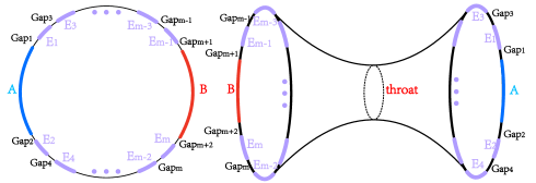
We first consider the case when and are two intervals on the spatial boundary in asymptotic AdS3. We assume that is a collection of intervals living in both the gap regions between and . The left side of Figure 1 depicts the configuration of such an in global coordinates. Using these connectivity conditions of the entanglement wedges, the formula of CMI reduces to
| (6) | ||||
where denotes the entanglement entropy of the gap region . In the second and third lines, III and I, II are used, respectively.
The vanishing of mutual information and in III implies that the surface homologous to has minimal area for the disconnected configuration rather than the connected configuration
| (7) |
The left-hand side of this inequality corresponds to the area of the surface homologous to which has a disconnected configuration, while the right-hand side corresponds to the area of the surface homologous to which has a connected configuration. This inequality gives an upper bound, which in turn gives CMI in formula (6) an upper bound as follows.
| (8) |
Assuming without loss of generality, this inequality can be saturated when reaches its phase transition point from the disconnected configuration to the connected configuration. When approaches infinity, the length of every single gap region goes to zero so that tends to zero and tends to . Thus, we have that approaches , its information-theoretical upper bound at last.
Therefore, for small distant subsystems and , the d.o.fs in all participate in the tripartite entanglement with and another carefully chosen region . We can make the following bold statement.
-
•
No Bell pairs exist in holographic states; all bipartite entanglement emerges from tripartite entanglement; any two distant small subsystems are highly tripartite entangling with another system.
We then analyze the upper bound of in the two-sided black hole geometry Maldacena and Susskind (2013); Susskind (2016), as shown on the right side of Figure 1. When and are on the same side of the black hole, the upper bound is the same as in asymptotic AdS3 through similar analysis. However, when and live in two different boundary CFTs, as we will see, the upper bound will be much less with no UV divergence due to the long-range entanglement Ju et al. (2024) involved. It is worth noting that in this case, I, II, and III are still valid as no specific background geometry is stipulated when proving them. As a result, (6) is still valid. The key step is still calculating the maximum value of , which is determined by the disconnectivity condition of , giving a different inequality in this case:
| (9) |
The right hand side corresponds to a partially connected configuration of where intervals of on the same boundary as region (right boundary in Figure 1) connect with , while the intervals of on the other boundary (left boundary in Figure 1) disconnect with . Using the symmetry of exchanging and , we have
| (10) |
Adding these two inequalities together, we have
| (11) | ||||
Note that this inequality can be saturated for sufficiently large but finite .
This is a surprising result, as we always take the throat as a symbol of bipartite entanglement between two CFT boundaries. However, we found that the throat area contributes to the tripartite entanglement between arbitrarily chosen sufficiently small regions and with another region . Compared with the result, this indicates the long-range nature in the tripartite global entanglement in .
After obtaining the upper bound of in the AdS3 and the two-sided black hole cases, we give a general formula for the value of the upper bound of in the following. In the most general case, e.g. when or has multiple intervals or in higher dimensions, formula (6) must still be satisfied. The only difference is that III will lead to different constraints on in general as follows
| (12) |
where the left-hand side still corresponds to the area of the disconnected configuration of . We define a region , , and is divided into two parts: one in and one in . The right-hand side corresponds to a partially connected configuration of where, inside region , is totally connected, while inside region , is disconnected.
According to the exchange symmetry of and , we can substitute and with and , respectively. We have
| (13) |
Adding these two inequalities together, we have
| (14) |
To make this upper bound as tight as possible, we need to be the minimal surface dividing from . As before, this upper bound can be infinitely approached when . This upper bound is the most general formula. We can check that in the two-sided black hole, is the entire side which contains , and in the global AdS3/CFT2, is either or , whichever has the smaller entanglement entropy, both giving the previous results.
In AdS4/CFT3, it can be proved that this general formula (14) is still valid; i.e., CMI approches when goes to infinity. Moreover, when (or ) is a concave region, the minimal surface that divides and will be the RT surface of the convex hull of (or ), instead of the RT surface of (or ) itself. This reveals the relationship between the convexity of the shape of the boundary region and the tripartite entanglement it participates in. Specifically, the UV degrees of freedom of region near the concave part (the part which is near but not near the boundary of the convex hull of ) cannot fully participate in the tripartite entanglement with a region outside the convex hull of .
We would like to impart a physical meaning to the area of the minimal surface in the context of holographic quantum information theory. The definition of the RT surface of is very similar to the definition of the entanglement wedge cross section (EWCS). In Takayanagi and Umemoto (2018), the EWCS between and is defined as the minimal surface that divides into two parts, with its area being conjectured to be the entanglement of purification (EoP) Terhal et al. (2002); Bagchi and Pati (2015) between and .
When is disconnected, no surface is needed to divide it into two parts. The area of the EWCS vanishes in this case, as does the EoP when to leading order in . However, in our case, does not vanish when . Instead, it is a large value. Therefore, it is not the traditional EoP, but rather the entanglement of state-constrained purification (EoSP) that we define as follows:
| (15) | ||||
The only difference between EoP and EoSP is that and are constrained to be boundary subregions in this holographic state instead of arbitrary extensions in quantum information theory. This constraint makes EoSP not the optimal choice from the viewpoint of EoP, resulting in it being significantly larger than EoP. We can easily prove that the value of EoSP we define is exactly , as the region is region .
Finally, we find the general tight upper bound of CMI
| (16) |
which can be saturated in general.
III The upper bound of
In this section, we analyze the upper bound of with , , fixed and arbitrarily chosen in holography. In quantum information theory, the amount of four-partite entanglement is independent of tripartite and bipartite entanglement among subsystems Ananth et al. (2015), and reaches its upper bound when tripartite entanglement vanishes. We could also stipulate the connectivity of the entanglement wedges as we did in the last section. The only difference is that the disconnectivity condition III should be modified as
| (17) |
The proof of this new constraint is tedious, but basically the same as we did for , which can be found in Appendix B. We only need to consider as a combination of intervals which satisfy those constraints to evaluate the upper bound of , which would be greatly simplified under these constraints
| (18) | ||||
As a result, calculating the upper bound of is still a problem of calculating the maximum value of , and the disconnectivity condition constrains its value from being too large.
Let us start from AdS3/CFT2 as shown on the left side in Figure 2. stipulates that
| (19) |
This inequality prevents the intervals inside from connecting with in , which would violate the disconnectivity condition. Using , we can get the other two inequalities as follows:
| (20) |
| (21) |
Adding these three inequalities together, combined with formula (25), we can get
| (22) | ||||
Finally, we get the upper bound of . Specifically, on the left side of Figure 2, this upper bound is the summation of the length of red curves minus the summation of the length of blue curves plus . We can find that the UV divergent terms of the red curves and the blue curves cancel out. As is an IR term, it will only finitely affect the value of . As a consequence, the upper bound of is definitely a finite value without UV divergence. This result can be generalized to general AdS3/CFT2 cases with , , and each being multiple intervals.
Let us calculate in higher-dimensional holography. As shown on the right side of Figure 2, is chosen as strips (annuli) which surround regions , , and . Formula (18) is still valid. The only difference is the constraint on imposed by the disconnectivity condition, which is
| (23) |
where is the gap adjacent to , which will be infinitely thin when tends to infinity. Rewriting the last inequality as
| (24) | ||||
Here, we assume that is minimal among {} without loss of generality. This upper bound can be saturated in a way similar to the last section.
At last, we conclude that given fixed and arbitrarily chosen, the upper bound of is finite in AdS3/CFT2 but infinite in higher-dimensional holography. This reveals the fundamental difference between the multipartite entanglement structure in low-dimensional holography and higher-dimensional holography. In higher-dimensional holographic CFT, any three distant local d.o.f.s are maximally participating in four-partite entanglement, while in AdS3/CFT2, the four-partite entanglement among them is sparse.
To further investigate the more-partite global entanglement structure that small distant regions participate, we can analyze the upper bound of under a generalized disconnectivity condition. Fortunately, in higher dimensional holography, we can always construct a configuration of the -th region such that, in this configuration reaches while any -partite entanglement for of the subregions with vanishes! This implies that these subregions fully participate in the -partite global entanglement, where all -partite entanglement among -partitions of these subregions arises from it Ju et al. (In progress). However, in AdS3/CFT2, is a summation of , and as has finite upper and lower bounds, the upper bound of will always be finite, i.e., -partite global entanglement is sparse among these subregions.
IV Conclusion
In this paper, we have investigated the tripartite entanglement structure in holographic states by evaluating the upper bound of that and participate. The general formula for the upper bound is which reaches the information theoretical upper bound in a wide class of and . Due to the properties at this upper bound, fully captures the tripartite global entanglement. As we have explained, this result reveals that all bipartite entanglement emerges from the tripartite entanglement in holographic states, and this conclusion can be generalized to -partite global entanglement in higher-dimensional holography. However, the upper bound of is finite in AdS3/CFT2, which reveals the fundamental difference in multipartite entanglement structure in different dimensions.
Acknowledgement
This work was supported by Project 12347183, 12035016 and 12275275 supported by the National Natural Science Foundation of China. It is also supported by Beijing Natural Science Foundation under Grant No. 1222031.
References
- Maldacena (1998) Juan Martin Maldacena, “The Large N limit of superconformal field theories and supergravity,” Adv. Theor. Math. Phys. 2, 231–252 (1998), arXiv:hep-th/9711200 .
- Ryu and Takayanagi (2006a) Shinsei Ryu and Tadashi Takayanagi, “Holographic derivation of entanglement entropy from the anti–de sitter space/conformal field theory correspondence,” Physical Review Letters 96 (2006a), 10.1103/physrevlett.96.181602.
- Akers and Rath (2020) Chris Akers and Pratik Rath, “Entanglement Wedge Cross Sections Require Tripartite Entanglement,” JHEP 04, 208 (2020), arXiv:1911.07852 [hep-th] .
- Walter et al. (2016) Michael Walter, David Gross, and Jens Eisert, “Multi-partite entanglement,” (2016), arXiv:1612.02437 [quant-ph] .
- Greenberger et al. (2007) Daniel M. Greenberger, Michael A. Horne, and Anton Zeilinger, “Going beyond bell’s theorem,” (2007), arXiv:0712.0921 [quant-ph] .
- Coffman et al. (2000) Valerie Coffman, Joydip Kundu, and William K. Wootters, “Distributed entanglement,” Phys. Rev. A 61, 052306 (2000), arXiv:quant-ph/9907047 .
- Bengtsson and Zyczkowski (2016) Ingemar Bengtsson and Karol Zyczkowski, “A brief introduction to multipartite entanglement,” arXiv preprint arXiv:1612.07747 (2016).
- Bao and Cheng (2019) Ning Bao and Newton Cheng, “Multipartite Reflected Entropy,” JHEP 10, 102 (2019), arXiv:1909.03154 [hep-th] .
- Yang et al. (2009) Dong Yang, Karol Horodecki, Michal Horodecki, Pawel Horodecki, Jonathan Oppenheim, and Wei Song, “Squashed entanglement for multipartite states and entanglement measures based on the mixed convex roof,” IEEE Transactions on Information Theory 55, 3375–3387 (2009).
- Yang et al. (2008) Dong Yang, Michał Horodecki, and Z. D. Wang, “An additive and operational entanglement measure: Conditional entanglement of mutual information,” Physical Review Letters 101 (2008), 10.1103/physrevlett.101.140501.
- Balasubramanian et al. (2024) Vijay Balasubramanian, Monica Jinwoo Kang, Chitraang Murdia, and Simon F. Ross, “Signals of multiparty entanglement and holography,” (2024), arXiv:2411.03422 [hep-th] .
- Bao et al. (2015) Ning Bao, Sepehr Nezami, Hirosi Ooguri, Bogdan Stoica, James Sully, and Michael Walter, “The Holographic Entropy Cone,” JHEP 09, 130 (2015), arXiv:1505.07839 [hep-th] .
- Hubeny et al. (2018) Veronika E. Hubeny, Mukund Rangamani, and Massimiliano Rota, “Holographic entropy relations,” Fortsch. Phys. 66, 1800067 (2018), arXiv:1808.07871 [hep-th] .
- Hubeny et al. (2019) Veronika E. Hubeny, Mukund Rangamani, and Massimiliano Rota, “The holographic entropy arrangement,” Fortsch. Phys. 67, 1900011 (2019), arXiv:1812.08133 [hep-th] .
- He et al. (2019) Temple He, Matthew Headrick, and Veronika E. Hubeny, “Holographic Entropy Relations Repackaged,” JHEP 10, 118 (2019), arXiv:1905.06985 [hep-th] .
- Hernández Cuenca (2019) Sergio Hernández Cuenca, “Holographic entropy cone for five regions,” Phys. Rev. D 100, 026004 (2019), arXiv:1903.09148 [hep-th] .
- He et al. (2020) Temple He, Veronika E. Hubeny, and Mukund Rangamani, “Superbalance of Holographic Entropy Inequalities,” JHEP 07, 245 (2020), arXiv:2002.04558 [hep-th] .
- Avis and Hernández-Cuenca (2023) David Avis and Sergio Hernández-Cuenca, “On the foundations and extremal structure of the holographic entropy cone,” Discrete Appl. Math. 328, 16–39 (2023), arXiv:2102.07535 [math.CO] .
- Fadel and Hernández-Cuenca (2022) Matteo Fadel and Sergio Hernández-Cuenca, “Symmetrized holographic entropy cone,” Phys. Rev. D 105, 086008 (2022), arXiv:2112.03862 [quant-ph] .
- Ju et al. (2023a) Xin-Xiang Ju, Bo-Hao Liu, Wen-Bin Pan, Ya-Wen Sun, and Yuan-Tai Wang, “Squashed Entanglement from Generalized Rindler Wedge,” (2023a), arXiv:2310.09799 [hep-th] .
- Ju et al. (2023b) Xin-Xiang Ju, Teng-Zhou Lai, Ya-Wen Sun, and Yuan-Tai Wang, “Holographic n-partite information in hyperscaling violating geometry,” JHEP 08, 064 (2023b), arXiv:2304.11430 [hep-th] .
- Guo and Zhang (2020) Yu Guo and Lin Zhang, “Multipartite entanglement measure and complete monogamy relation,” Physical Review A 101 (2020), 10.1103/physreva.101.032301.
- Erdmenger et al. (2017) Johanna Erdmenger, Daniel Fernandez, Mario Flory, Eugenio Megias, Ann-Kathrin Straub, and Piotr Witkowski, “Time evolution of entanglement for holographic steady state formation,” JHEP 10, 034 (2017), arXiv:1705.04696 [hep-th] .
- Araki and Lieb (1970) Huzihiro Araki and Elliott H Lieb, “Entropy inequalities,” Communications in Mathematical Physics 18, 160–170 (1970).
- Shirokov (2017) M. E. Shirokov, “Tight uniform continuity bounds for the quantum conditional mutual information, for the holevo quantity, and for capacities of quantum channels,” Journal of Mathematical Physics 58 (2017), 10.1063/1.4987135.
- Ryu and Takayanagi (2006b) Shinsei Ryu and Tadashi Takayanagi, “Aspects of Holographic Entanglement Entropy,” JHEP 08, 045 (2006b), arXiv:hep-th/0605073 .
- Headrick (2019) Matthew Headrick, “Lectures on entanglement entropy in field theory and holography,” (2019), arXiv:1907.08126 [hep-th] .
- Hayden et al. (2013) Patrick Hayden, Matthew Headrick, and Alexander Maloney, “Holographic mutual information is monogamous,” Physical Review D 87 (2013), 10.1103/physrevd.87.046003.
- Cui et al. (2019) Shawn X. Cui, Patrick Hayden, Temple He, Matthew Headrick, Bogdan Stoica, and Michael Walter, “Bit Threads and Holographic Monogamy,” Commun. Math. Phys. 376, 609–648 (2019), arXiv:1808.05234 [hep-th] .
- Czech et al. (2012) Bartlomiej Czech, Joanna L. Karczmarek, Fernando Nogueira, and Mark Van Raamsdonk, “The Gravity Dual of a Density Matrix,” Class. Quant. Grav. 29, 155009 (2012), arXiv:1204.1330 [hep-th] .
- Wall (2014) Aron C. Wall, “Maximin Surfaces, and the Strong Subadditivity of the Covariant Holographic Entanglement Entropy,” Class. Quant. Grav. 31, 225007 (2014), arXiv:1211.3494 [hep-th] .
- Headrick et al. (2014) Matthew Headrick, Veronika E. Hubeny, Albion Lawrence, and Mukund Rangamani, “Causality & holographic entanglement entropy,” JHEP 12, 162 (2014), arXiv:1408.6300 [hep-th] .
- Maldacena and Susskind (2013) Juan Maldacena and Leonard Susskind, “Cool horizons for entangled black holes,” Fortsch. Phys. 61, 781–811 (2013), arXiv:1306.0533 [hep-th] .
- Susskind (2016) Leonard Susskind, “ER=EPR, GHZ, and the consistency of quantum measurements,” Fortsch. Phys. 64, 72–83 (2016), arXiv:1412.8483 [hep-th] .
- Ju et al. (2024) Xin-Xiang Ju, Teng-Zhou Lai, Bo-Hao Liu, Wen-Bin Pan, and Ya-Wen Sun, “Entanglement structures from modified IR geometry,” JHEP 07, 181 (2024), arXiv:2404.02737 [hep-th] .
- Takayanagi and Umemoto (2018) Tadashi Takayanagi and Koji Umemoto, “Entanglement of purification through holographic duality,” Nature Phys. 14, 573–577 (2018), arXiv:1708.09393 [hep-th] .
- Terhal et al. (2002) Barbara M. Terhal, Michał Horodecki, Debbie W. Leung, and David P. DiVincenzo, “The entanglement of purification,” Journal of Mathematical Physics 43, 4286–4298 (2002).
- Bagchi and Pati (2015) Shrobona Bagchi and Arun Kumar Pati, “Monogamy, polygamy, and other properties of entanglement of purification,” Physical Review A 91 (2015), 10.1103/physreva.91.042323.
- Ananth et al. (2015) N. Ananth, V. K. Chandrasekar, and M. Senthilvelan, “Criteria for non-k-separability of n-partite quantum states,” The European Physical Journal D 69 (2015), 10.1140/epjd/e2015-50538-5.
- Ju et al. (In progress) Xin-Xiang Ju, Wen-Bin Pan, Ya-Wen Sun, Yuan-Tai Wang, and Yang Zhao, (In progress).
Appendix A Proof of the disconnectivity condition for
In this appendix, we prove the disconnectivity condition as follows. Given a configuration with a non-vanishing or , there always exists a disconnected configuration of with vanishing and whose CMI is not less than the former one.
Note that we do not demand that the disconnected configuration has the same as the connected configuration. One can choose a configuration with many times larger than that of the connected configuration, as long as its CMI is not less.
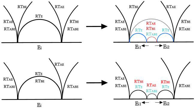
Let us prove it in the general situation. There are four steps to prove this theorem. According to Figure 3, we start from one of the intervals of , written as , whose entanglement wedge is connected with both and in the configuration of and . We split from the middle into two subregions and by adding a gap inside while preserving the outer boundary of unchanged. When the gap is very small, the and are fully connected in , and as we have argued in the proof of condition II, the value of CMI does not change after opening this small gap.
The second step: when we continuously enlarge the gap, the first phase transition of the entanglement wedge occurs, which makes and disconnected in , while preserving the connectivity of and in and . This is shown in Figure 3.
The third step: we continuously enlarge the gap inside . One can find that and both decrease, while the entropy of the gap region in-between increases. These three quantities are the only ones that affect the value of CMI because the outer boundary of remains unchanged. The sign of them inside is drawn as the different colors of those RT surfaces in Figure 3; red represents positive and blue represents negative. It is easy to observe that when we enlarge the gap, CMI increases until another phase transition occurs. In principle, the phase transition could occur on one of or , i.e. suddenly becomes disconnected between and while remaining the connectivity between and (Here, we assume that and become disconnected in before and become disconnected in , without loss of generality.). However, we can make the phase transition occur on and simultaneously by adjusting the middle point of this gap. Note that if the middle point of the gap region between and is far left inside the original region , disconnects with first; otherwise, if the middle point is far right inside the original region , disconnects with first. Therefore, there must exist a fine-tuned middle point which makes the phase transition occur on and simultaneously. After the phase transition, and disconnect with in . Remember that when we enlarge the gap, the CMI increases, so we prove that: for a configuration whose intervals of connect with both and inside and respectively, one can always find another configuration whose intervals connect to at most one of and inside and , with larger CMI.
After performing the third step for all the intervals of , we are left with a configuration where all intervals of only connect with in or only connect with in . The fourth step is to consider an interval which is only connected with in , and find another disconnected configuration with CMI not less than it. To achieve this final goal, we have to split again. In the second line of Figure 3, this process is illustrated. The only difference is that the CMI will not change no matter how we enlarge the gap, as long as and are connected in . Again, we can make the phase transition occur between and and between and simultaneously. At the end, both and are disconnected from . Combining with the last three steps, in the end, we find a disconnected configuration with CMI not less than that of the connected configuration, and the disconnectivity condition is proven. Note that this proof is valid for various geometries and in higher-dimensional cases. When is a disk, the “gap” inside region would be a disk; when is an annulus, the gap would be an annulus that splits into two annuli, etc.
Appendix B Proof of the disconnectivity condition for
The disconnectivity condition in is a stronger generalization of that in , which states that only analyzing the disconnected case which satisfies
| (25) |
is enough to evaluate the upper bound of . In other words, for a connected configuration of which does not satisfy formula (25), there always exists a disconnected configuration whose is not less.
To prove this theorem, we split the interval which connects to at least one of , , and in or or into two pieces, and , as we did in the last section. Figure 4 presents this whole procedure.
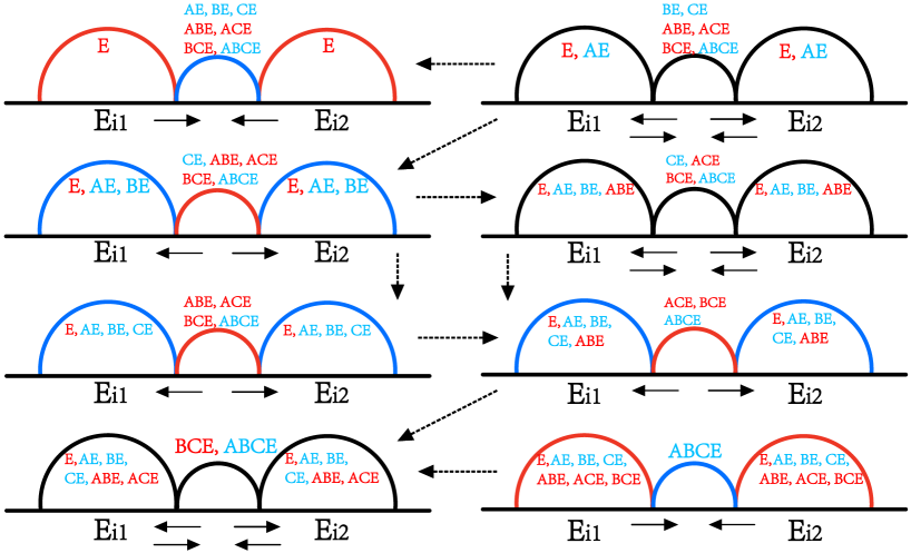
In this figure, each of the eight diagrams presents a case where interval is split into two halves and . When the position of the endpoints of the gap is modified, only the area of three minimal surfaces (semicircles in the figure) changes to affect . According to formula (1), there are eight terms in which contain : , , , , , , , and , respectively. Each of those RT surfaces contains the semicircles in those figures and are labeled on those semicircles. Red and blue represent the positivity of the term in , and the color of the circle represents the positivity of the summation of all RT surfaces labeled on this circle (black means that the area of this circle cancels out in ). The black arrows below the endpoints of gaps between and represent the direction of the modification of those endpoints that enlarges the . The dashed arrows between each diagram represent the direction of increasing .
Let us analyze these cases one by one.
The first case is when connects with or or in all entanglement wedges except . As shown in diagram (1.1), splitting into and with a gap between them will decrease , as one should decrease the length of the gap to make the length of the blue curve decrease and the length of red curves increase in order to increase . The second case is that only disconnects with in entanglement wedge while connecting with or or in all other entanglement wedges, as shown in diagram (1.2). In this case, moving the endpoints of the gap between and will not modify , so we can enlarge the gap between and until the phase transition of occurs to and simultaneously and make the entanglement wedge disconnected, which is shown in diagram (1.3). We can split , which disconnects with and in the entanglement wedges of and while connecting with other entanglement wedges, again. This time, splitting will increase to diagram (2.2) or diagram (3.1). Splitting again, diagram (2.2) or diagram (3.1) will lead to diagram (3.2). Splitting diagram (3.2) will lead to diagram (4.1). However, splitting diagram (4.1) will decrease . As a result, the maximum of might be chosen as the configuration between diagram (4.1) and (4.2), which is the phase transition point. In this case, disconnects with , , and in the entanglement wedges of , , and , which satisfies the disconnectivity condition.
From the above argument, we can see that in the disconnected configuration reaches the maximum among all diagrams except diagram (1.1). So we are one step closer to proving the disconnectivity condition. The next step is to rule out the possibility of diagram (1.1) being the diagram with the maximum . However, this task seems difficult. Instead, we have
| (26) |
where is the complement of region . We can find that when are fixed regions, if reaches the upper bound, must reach the lower bound. As a result, we could try to find the configuration of with the minimal value of . Then, according to equation (26), will make reach the upper bound.
The procedure of finding the minimal value is exactly the opposite of finding the maximum value. One just has to reverse all arrows in Figure 4. As we already analyzed before, it is easy to find that there are two configurations which might reach the minimal value: diagram (1.2) and diagram (4.2). Let us analyze diagram (4.2) first. One should enlarge the gap between and in order to decrease . At last, could be disconnected and reaches its minimal value. However, in this case, intervals and disconnect with all entanglement wedges. We have argued that this case will lead to the result that eliminating and will not affect the CMI. This argument is still valid in the case. Until now, we understand why diagram (4.2) will reach the local minimal value of , because it is zero, and the real lower bound must be negative. So, only diagram (1.2) has the right to become the configuration with minimal . As adjusting the length of the gap will not change , we can shorten it until a phase transition between diagram (1.1) and (1.2) happens, in which case, connects with or or in all entanglement wedges. In this diagram, we mark as the region that purifies ; then is the collection of gaps between and , and the connectivity of , , and is equivalent to the disconnectivity of , , and , respectively. From equation (26), must be the region that maximizes , and the disconnectivity condition (25) is proven.