Elastic-Degenerate String Comparison††thanks: This work was partially supported by the PANGAIA, ALPACA and NETWORKS projects that have received funding from the European Union’s Horizon 2020 research and innovation programme under the Marie Skłodowska-Curie grant agreements No. 872539, 956229 and 101034253, respectively. Nadia Pisanti was partially supported by MUR PRIN 2022 YRB97K PINC and by NextGeneration EU programme PNRR ECS00000017 Tuscany Health Ecosystem. Jakub Radoszewski was supported by the Polish National Science Center, grants no. 2018/31/D/ST6/03991 and 2022/46/E/ST6/00463.
Abstract
An elastic-degenerate (ED) string is a sequence of sets containing strings in total whose cumulative length is . We call , , and the length, the cardinality and the size of , respectively. The language of is defined as . ED strings have been introduced to represent a set of closely-related DNA sequences, also known as a pangenome. The basic question we investigate here is: Given two ED strings, how fast can we check whether the two languages they represent have a nonempty intersection? We call the underlying problem the ED String Intersection (EDSI) problem. For two ED strings and of lengths and , cardinalities and , and sizes and , respectively, we show the following:
-
•
There is no -time algorithm, thus no -time algorithm and no -time algorithm, for any constant , for EDSI even when and are over a binary alphabet, unless the Strong Exponential-Time Hypothesis is false.
-
•
There is no combinatorial -time algorithm, for any constant and any function , for EDSI even when and are over a binary alphabet, unless the Boolean Matrix Multiplication conjecture is false.
-
•
An -time algorithm for outputting a compact (RLE) representation of the intersection language of two unary ED strings. In the case when and are given in a compact representation, we show that the problem is NP-complete.
-
•
An -time algorithm for EDSI.
-
•
An -time algorithm for EDSI, where is the exponent of matrix multiplication; the notation suppresses factors that are polylogarithmic in the input size.
We also show that the techniques we develop here have many applications even outside of bioinformatics.
1 Introduction
Sequence (or string) comparison is a fundamental task in computer science, with numerous applications in computational biology [37], signal processing [25], information retrieval [10], file comparison [38], pattern recognition [6], security [53], and elsewhere [54]. Given two or more sequences and a distance function, the task is to compare the sequences in order to infer or visualize their (dis)similarities [23].
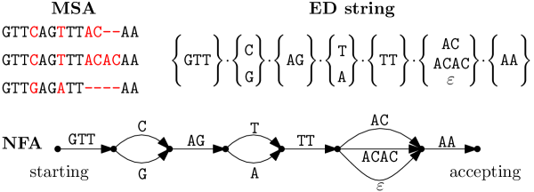
Many sequence representations have been introduced over the years to account for unknown or uncertain letters, a phenomenon that often occurs in data that comes from experiments [12]. In the context of computational biology, for example, the IUPAC notation [42] is used to represent loci in a DNA sequence for which several alternative nucleotides are possible as variants. This gives rise to the notion of degenerate string (or indeterminate string): a sequence of finite sets of letters [3]. When all sets are of size 1, we are in the special case of a standard string (or deterministic string). Degenerate strings can encode the consensus of a population of DNA sequences [26] in a gapless multiple sequence alignment (MSA). Iliopoulos et al. generalized this notion to also encode insertions and deletions (gaps) occurring in MSAs by introducing the notion of elastic-degenerate string: a sequence of finite sets of strings [39].
The main motivation to consider elastic-degenerate (ED) strings is that they can be used to represent a pangenome: a collection of closely-related genomic sequences that are meant to be analyzed together [58]. Several other, more powerful, pangenome representations have been proposed in the literature, mostly graph-based ones; see the comprehensive survey by Carletti et al. [20] or by Baaijens et al. [7]. Compared to these more powerful representations, ED strings have algorithmic advantages, as they support: (i) fast and simple on-line string matching [36, 21]; (ii) (deterministic) subquadratic string matching [4, 14, 15]; and (iii) efficient approximate string matching [16, 13].
Our main goal here is to give the first algorithms and lower bounds for comparing two pangenomes represented by two ED strings.111Pangenome comparison is one of the central goals of two large EU funded projects on computational pangenomics: PANGAIA (https://www.pangenome.eu/) and ALPACA (https://alpaca-itn.eu/). We consider the most basic notion of matching, namely, to decide whether two ED strings, each encoding a language, have a nonempty intersection. Like with standard strings, algorithms for pairwise ED string comparison can serve as computational primitives for many analysis tasks (e.g., phylogeny reconstruction); lower bounds for pairwise ED string comparison can serve as meaningful lower bounds for the comparison of more powerful pangenome representations such as, for instance, variation graphs [20].
Let us start with some basic definitions and notation. An alphabet is a finite nonempty set of elements called letters. By we denote the set of all strings over including the empty string of length . For a string over , we call its length. The fragment of is an occurrence of the underlying substring . We also say that occurs at position in . A prefix of is a fragment of of the form and a suffix of is a fragment of of the form . An elastic-degenerate string (ED string, in short) is a sequence of finite sets, where is a subset of . The total size of is defined as , where is the total number of empty strings in . By we denote the total number of strings in all , i.e., . We say that has length , cardinality and size . An ED string can be treated as a compacted nondeterministic finite automaton (NFA) with states, called segments, numbered , and transitions labeled by strings in . State is starting and state is accepting. For each index and string , there is a transition from state to state with label ; inspect also Fig. 1 for an example. The language generated by the ED string is the language accepted by this compacted NFA. That is, .
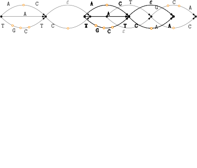
We next define the main problem in scope; inspect also Figure 2 for an example.
ED String Intersection (EDSI) Input: Two ED strings, of length , cardinality and size , and of length , cardinality and size . Output: YES if and have a nonempty intersection, NO otherwise.

Our Results
We make the following specific contributions:
-
1.
In Section 2.1, we give several conditional lower bounds. In particular, we show that there is no -time algorithm, thus no -time algorithm and no -time algorithm, for any constant , for EDSI even when and are over a binary alphabet, unless the Strong Exponential-Time Hypothesis (SETH) [40, 41] or the Orthogonal Vectors (OV) conjecture [62] is false.
-
2.
In Section 2.2, we present other conditional lower bounds. In particular, we show that there is no combinatorial222The notion of “combinatorial algorithm” is informal but widely used in the literature. Typically, we call an algorithm “combinatorial” if it does not not call an oracle for ring matrix multiplication. -time algorithm, for any constant and any function , for EDSI even when and are over a binary alphabet, unless the Boolean Matrix Multiplication (BMM) conjecture [1] is false.
-
3.
In Section 3, we show an -time algorithm for outputting a compact (RLE) representation of the intersection language of two unary ED strings. In the case when and are given in a compact representation, we show that the problem is NP-complete.
-
4.
In Section 4.1, we show an -time combinatorial algorithm for EDSI in which we assume that the ED strings are over an integer alphabet .
-
5.
In Section 4.2, we show an -time algorithm for EDSI, where is the matrix multiplication exponent.
Interestingly, we show that the techniques we develop here have applications outside of bioinformatics. Given a sequence of standard strings, we define an acronym of as a string , where is a possibly empty prefix of , for all . In the Acronym Generation (AG) problem, we are given a dictionary of strings of total length and a sequence of strings of total length , and we are asked to say YES if and only if some acronym of belongs to . In Section 5, we show how our techniques for EDSI can be modified to solve AG in time.
In Section 6, we show how intersection graphs can be used to solve different ED string comparison tasks. In Section 7, we show how intersection graphs can be used for string matching in the general case when both the pattern and the text are ED strings. In Section 8, we extend our results for EDSI to the approximate case (under the Hamming or edit distance). We conclude this paper in Section 9 with some open problems.
This is a full and extended version of a conference paper [31].
Related Work
Apart from its applications to pangenome comparison, EDSI is interesting theoretically on its own as a special case of regular expression (regex) matching. Regex is a basic notion in formal languages and automata theory. Regular expressions are commonly used in practical applications to define search patterns. Regex matching and membership testing are widely used as computational primitives in programming languages and text processing utilities (e.g., the widely-used agrep). The classic algorithm for solving these problems constructs and simulates an NFA corresponding to the regex, which gives an running time, where is the length of the pattern and is the length of the text. Unfortunately, significantly faster solutions are unknown and unlikely [8]. However, much faster algorithms exist for many special cases of the problem: dictionary matching, wildcard matching, subset matching, and the word break problem (see [8] and references therein) as well as for sparse regex matching [17].
Special cases of EDSI have also been studied. First, let us consider the case when both and are degenerate strings. In this case, the problem is trivial: EDSI has a positive answer if and only if for every , is nonempty. Alzamel et al. [2, 3] studied the case when and are generalized degenerate strings: for any and all strings in have the same length and all strings in have the same length . In the case of generalized degenerate strings, they showed that deciding if and have a nonempty intersection can be done in time. If is a standard string, i.e., an ED string with , then we can resort to the results of Bernardini et al. [15] for ED string matching. In particular: there is no combinatorial algorithm for EDSI working in time unless the BMM conjecture is false; and we can solve EDSI in time. Moreover, Gawrychowski et al. [34] provided a systematic study of the complexity of degenerate string comparison under different notions of matching: Cartesian tree matching; order-preserving matching; and parameterized matching.
Similar to ED strings (and to generalized degenerate strings) is the representation of pangenomes via founder graphs. The idea behind founder graphs is that a multiple alignment of few founder sequences can be used to approximate the input MSA, with the feature that each row of the MSA is a recombination of the founders. Like founder graphs, ED strings support the recombination of different rows of the MSA between consecutive columns. Unlike ED strings, for which no efficient index is probable [35] (and indeed their value is to enable fast on-line string matching), some subclasses of founder graphs are indexable, and a recent research line is devoted to constructing and indexing such structures [5, 28, 52, 55]. In general, both ED strings and founder graphs are special cases of labeled graphs. Unfortunately, indexing labeled graphs is unlikely to have an efficient solution [27].
2 Conditional Lower Bounds
In this section, we show several conditional lower bounds for the EDSI problem. Bounds in the first group (see Section 2.1) are based on the popular Strong Exponential-Time Hypothesis (SETH) [19]; the second group of bounds (see Section 2.2) is based, instead, on the Boolean Matrix Multiplication (BMM) conjecture [1].
2.1 Lower Bounds Based on SETH
We are going to reduce the Orthogonal Vectors (OV, in short) problem to the EDSI problem. In the OV problem we are given a set of binary vectors, each of length , and we are asked to decide whether or not there are any two vectors in which are orthogonal; i.e., the dot product of the two vectors is zero. The OV conjecture, implied by SETH (see [62]), is the following.
Conjecture 2.1 (OV conjecture [62]).
The OV problem for binary vectors, each of length , cannot be solved in time, for any constant .
We show the following reduction.
Theorem 2.2.
Given any set of binary vectors of length , we can construct in linear time two ED strings and over a binary alphabet such that:
-
•
has length, cardinality, and size ;
-
•
has length , cardinality and size ; and
-
•
contains two orthogonal vectors if and only if and have a nonempty intersection.
Proof.
Let for all . For a length- vector and , by we denote the th component of . We construct and as follows (see Example 2.3):333By the notation we denote a sequence of concatenations of segments in an ED string.
We now show that and have a nonempty intersection if and only if there exists a pair of orthogonal vectors in .
-
•
Suppose and are orthogonal. Then for all , and hence . It follows that
By decomposing and , where for any integer , the set contains the positions with a in the binary representation of , we find that
We conclude that .
-
•
Conversely, suppose that and have a nonempty intersection and consider a string . Let be the vector from which is chosen in when constructing . The strings in the sets of all have length divisible by . Thus starts at an index of string for some integer . Since , we have . This implies that and are orthogonal.
Therefore, solving the orthogonal vectors problem for is equivalent to checking whether and have a nonempty intersection. ∎
Example 2.3.
Let , and .
We have that
and .
One can observe that each string from corresponds to a pair of orthogonal vectors from . For example, the string is in because . Since the vector is orthogonal to , one also has . This is because the two first segments of are constructed to encode any vector which is orthogonal to .
Note that when , the length , the cardinality and the size of are , whereas has length , cardinality and size . Moreover, both ED strings are over a binary alphabet . This implies various hardness results for EDSI. For example, we can see that, for any constant , and an alphabet of size at least the problem cannot be solved in
time, conditional on the OV conjecture. By using the fact that and , we obtain the following bounds.
Corollary 2.4.
For any constant , there exists no
-
•
-time
-
•
-time
-
•
-time
algorithm for the EDSI problem, unless the OV conjecture is false.
2.2 Combinatorial Lower Bounds Based on BMM Conjecture
In the Triangle Detection (TD, in short) problem we are given three Boolean matrices , , and one has to check whether there are three indices such that . It is known that Boolean Matrix Multiplication (BMM) and TD either both have truly subcubic combinatorial algorithms or none of them do [59]. The BMM conjecture is stated as follows.
Conjecture 2.5 (BMM conjecture [1]).
Given two Boolean matrices, there is no combinatorial algorithm for BMM working in time, for any constant .
Our reduction from TD to EDSI is based on the construction of Bernardini et al. from [15] for ED string matching.
Theorem 2.6.
If EDSI over a binary alphabet can be solved in time, for any constant and any function , then there exists a truly subcubic combinatorial algorithm for TD.
Proof.
Let be a positive integer and let , , and be three Boolean matrices. Further let be an integer to be set later. In the rest of the proof, we can assume that divides , up to adding rows and columns containing only ’s to all three matrices, where is the smallest non-negative representative of the equivalence class .
Let us first construct an ED string over a large alphabet with , where each , , contains a string for each occurrence of value in , and , respectively. Below iterates over , and iterate over , and and iterate over . Moreover, , for , and , are all letters.
-
•
If , then contains the string .
-
•
If , then contains the string .
-
•
If , then contains the string .
The length of each string in each is and the total number of strings is up to . Overall, .
We construct an ED string with containing the following strings:
Each string has length and there are strings, so .
We use the following fact.
Fact 2.7 ([15]).
if and only if the following holds for some :
We choose ; then and . Then indeed an -time algorithm for EDSI would yield an -time algorithm for the TD problem.
Note also that even though the size of the alphabet used above is , we can encode all letters by equal-length binary strings blowing and up only by a factor of and, hence, obtain the same lower bound for a binary alphabet. ∎
Both and in the reduction are , thus an -time algorithm would yield an -time algorithm for TD. We obtain the following.
Corollary 2.8.
If EDSI over a binary alphabet can be solved in time, for any constant and any function , then there exists a truly subcubic combinatorial algorithm for TD.
3 EDSI: The Unary Case
An ED string is called unary if it is over an alphabet of size 1. In this special case, if both and are over the same alphabet , EDSI boils down to checking whether there exists any such that belongs to both and .
Let be a unary ED string of length over alphabet . We define the compact representation of as the following sequence of sets of integers:
where for all and , the cardinality of is , and its size is , where is the total number of empty strings in .
Theorem 3.1.
If and are unary ED strings and each is given in a compact representation, the problem of deciding whether is nonempty is NP-complete.
Proof.
The problem is clearly in NP, as it is enough to guess a single element for each set in both and , and then simply check if the sums match in linear time. We show the NP-hardness through a reduction from the Subset Sum problem, which takes integers and an integer , and asks whether there exist , for all , such that . Subset Sum is NP-complete [45] also for non-negative integers. For any instance of Subset Sum, we set for all , and . Then the answer to the Subset Sum instance is YES if and only if is nonempty. ∎
In what follows, we provide an algorithm which runs in polynomial time in the size of the two unary ED strings when they are given uncompacted.
The set can be represented as a set such that . The set will be stored as a sorted list (without repetitions). We will show how to efficiently compute and . Then one can compute in time, which allows, in particular, to check if (which is equivalent to ).
We show the computation for . The workhorse is an algorithm from the following Lemma 3.2 that allows to compute the set of concatenation of two ED strings based on their sets .
Lemma 3.2.
Let and be ED strings. Given and such that and , we can compute in time.
Proof.
For two sets , by we denote the set . We then have . Fast Fourier Transform (FFT) [22] can be used directly to compute in time. ∎
Lemma 3.3.
can be computed in time.
Proof.
We apply the recursive algorithm described in Algorithm 1 to .
Let and for . Obviously, .
We analyze the complexity of the recursion by levels. For the bottom level, can be computed in time for each , which sums up to . For the remaining levels, we notice that . On each level, the fragments of that are considered are disjoint. Thus, the complexity on each level via Lemma 3.2 is . The number of levels of recursion is ; the complexity follows. ∎
Theorem 3.4.
If and are unary ED strings, then can be computed in time.
Proof.
We use Lemma 3.3 to compute and in the required complexity. Then can be computed via bucket sort. ∎
4 EDSI: General Case
Assuming that the two ED strings, and , of total size are over an integer alphabet , we can sort the suffixes of all strings in , for all , and the suffixes of all strings in , for all , in time [29].
By let us denote the length of the longest common prefix of two strings and . Given a string over an integer alphabet, we can construct a data structure over in time, so that when are given to us on-line, we can determine in time [11].
4.1 Compacted NFA Intersection
In this section we show an algorithm for computing a representation of the intersection of the languages of two ED strings using techniques from formal languages and automata theory.
Definition 4.1 (NFA).
A nondeterministic finite automaton (NFA) is a 5-tuple , where is a finite set of states; is an alphabet; is a transition function, where is the power set of ; is the starting state; and is the set of accepting states.
Using the folklore product automaton construction, one can check whether two NFA have a nonempty intersection in time, where and are the sizes of the two NFA [50]. We use a different, compacted representation of automata, which in some special cases allows a more efficient algorithm for computing and representing the intersection.
Definition 4.2 (Compacted NFA).
An extended transition is a transition function of the form , where is a finite set of states, is the set of strings over alphabet , and is the power set of . A compacted NFA is an NFA in which we allow extended transitions. Such an NFA can also be represented by a standard (uncompacted) NFA, where each extended transition is subdivided into standard one-letter transitions (and -transitions), . The states of the compacted NFA are called explicit, while the states obtained due to these subdivisions are called implicit.
Given a compacted NFA with explicit states and extended transitions, we denote by and the number of states and transitions, respectively, of its uncompacted version . Henceforth we assume that in the given NFA every state is reachable, and hence we have and .
Lemma 4.3.
Given two compacted NFA and , with and explicit states and and extended transitions, respectively, a compacted NFA representing the intersection of and with explicit states and extended transitions can be computed in time if and are over an integer alphabet .
Proof.
We start by constructing an LCP data structure over the concatenation of all the labels of extended transitions of both NFA of total size . It requires -time preprocessing and allows answering LCP queries on any two substrings of such labels in time.
We construct , a compacted NFA representing the intersection of and .
Every state of is composed of a pair: an explicit state of one automaton and any explicit or implicit state of the other automaton (or equivalently a state of the uncompacted version of the automaton). Thus the total number of explicit states of is .
We need to compute the extended transitions of . For a state we check every string pair , where iterates over all extended transitions going out of and iterates over all extended transitions going out of (a transition going out of an implicit state is represented by a suffix of the transition it belongs to). For every pair we ask an query. If is equal to one of , (possibly both), we create an extended transition between and the pair of states reachable through those transitions (if one of the transitions is strictly longer, we prune it to the right length, ending it at an implicit state of its input NFA). Otherwise such a transition does not lead to any explicit state of and thus cannot be used to reach the accepting state; hence we ignore it.
Finally, the starting (resp. accepting) state of corresponds to a pair of starting (resp. accepting) states of and .
Since any pair representing an explicit state of contains an explicit state of or , the number of such transition pair checks (and hence also the number of the extended transitions of ) is . Since each such check takes time, the construction complexity follows. Note that NFA may contain unreachable states; such states can be removed afterwards in linear time. The algorithms’ correctness follows from the observation that is in fact the standard intersection automaton of and with some states, that do not belong to any path between the starting and the accepting states, removed. ∎

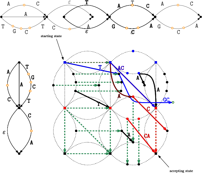
We next define the path-automaton of an ED string (inspect Fig. 3 for an example).
Definition 4.4 (Path-automaton).
Let be an ED string of length , cardinality , and size . The path-automaton of is the compacted NFA consisting of:
-
•
explicit states, numbered from through . State is the starting state and state is the accepting state. State is the state in-between and .
-
•
extended transitions from state to state labeled with the strings in , for all , where .
The path-automaton of accepts exactly . The uncompacted version of this path-automaton has states and transitions.
An example is constructed in Figure 4.
Lemma 4.3 thus implies the following result.
Corollary 4.5.
The compacted NFA representing the intersection of two path-automata with explicit states and extended transitions can be constructed in time if the path-automata are over an integer alphabet.
Theorem 4.6.
EDSI for ED strings over an integer alphabet can be solved in time. If the answer is YES, a witness can be reported within the same time complexity.
Proof.
The path-automaton of an ED string of size can be constructed in time. Given two ED strings, we can construct their path-automata in linear time and apply Corollary 4.5. By finding any path in the intersection automaton from the starting to the accepting state in linear time (if it exists), we obtain the result. The construction is detailed on an example in Figure 5 ∎
Notice that the path-automata representing ED strings, as well as their intersection, are always acyclic, but may contain -transitions. In the following we are only interested in the graph underlying the path-automaton, that is the directed acyclic graph (DAG), where every node represents an explicit state and every labeled directed edge represents an extended transition of the path-automaton (inspect also Fig. 1).
4.2 An -time Algorithm for EDSI
In this section, we start by showing a construction of the intersection graph computed by means of Lemma 4.3 in the case when the input is a pair of path-automata that allows an easier and more efficient implementation. The construction is then adapted to obtain an -time algorithm for solving the EDSI problem.
For by we denote the compacted NFA (henceforth, graph ) representing the ED string . By we denote the set of implicit states (henceforth, implicit nodes) appearing on the extended transitions (henceforth, edges) between explicit states (henceforth, explicit nodes) and . For convenience, the implicit nodes in the sets can be numbered consecutively starting from .
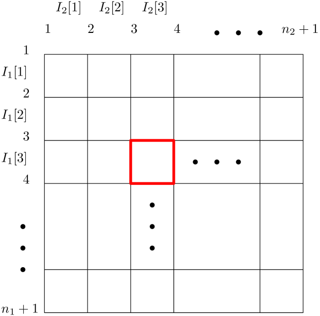
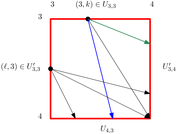
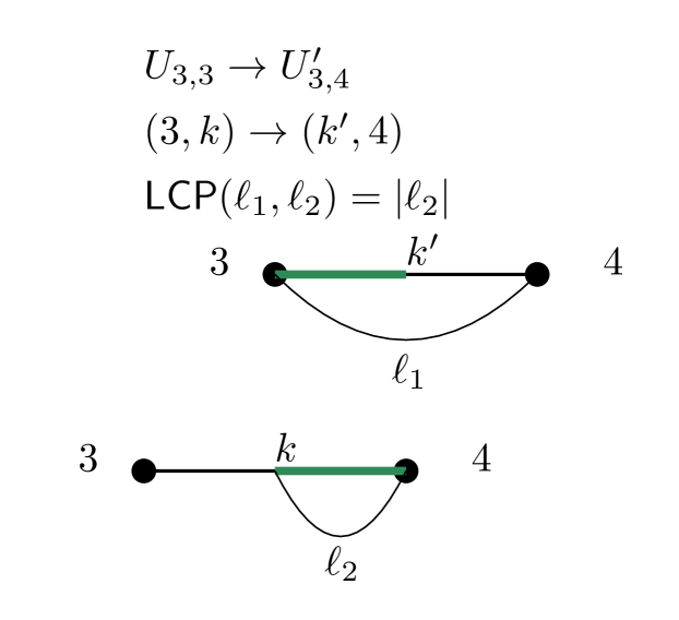
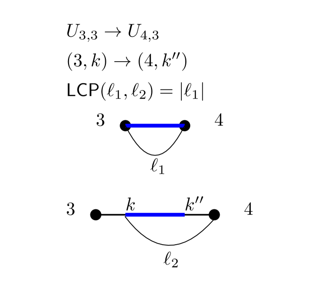
Let and , for all and . As in the construction of Lemma 4.3, the union of all and is the set of explicit nodes of the intersection graph that we construct; this can be represented graphically by a grid, where the horizontal and vertical lines correspond to and , respectively (inspect Fig. 6(a)). In particular, we would like to compute the edges between these explicit nodes (inspect Fig. 6(b)) in time.
Consider an explicit node of the intersection graph; this node is represented by a pair of nodes: one from and one from . We need to consider two cases: explicit vs explicit node; or explicit vs implicit node. By symmetry, it suffices to consider an explicit first node. Let us denote this pair by , where is an explicit node of and is a node of . Let us further denote by the label of one of the edges going from node to node . For , we have two cases. If is explicit (i.e., ) then we denote by the label of one of the edges going from to . Otherwise ( is implicit), we denote by the path label (concatenation of labels) from node to node .
As noted in the proof of Lemma 4.3, an edge is constructed only if . If (a prefix of a string in is equal to the suffix of a string in starting at the position corresponding to node ), the edge ends in a node from (Fig. 6(c)). If (a whole string from occurs in a string from starting at the position corresponding to node ), the edge ends in a node from (Fig. 6(d)). Otherwise (; the two strings are equal) the edge ends in . Symmetrically (i.e., the second node is explicit), the edge going out of a node from ends at a node from the set (inspect Fig. 6(b)).
We next show how to construct the intersection graph by computing all such edges going out of or in a single batch using suffix trees (inspect Fig. 7 for an example). This construction allows an easier and more efficient implementation in comparison to the LCP data structure used in the general NFA intersection construction. Let us recall that denotes the size of the ED string . Henceforth we denote for and for .
Lemma 4.7.
For any and , we can construct all edges going out of nodes in in time using the generalized suffix tree of the strings in . We assume that the letters of strings in are over an integer alphabet .
Proof.
Let us start with a simple implementation of the lemma that works with high probability. We will then give the details for a deterministic implementation.
We first construct the generalized suffix tree of the strings in in time [29]. We also mark each node corresponding to a suffix of a string in with a -label. Each such node is also decorated with one or multiple starting positions, respectively, from one or multiple elements of sharing the same suffix. For each branching node of the suffix tree, we construct a hash table, to ensure that any outgoing edge can be retrieved in constant time based on the first letter (the key) of its label. This can be done in time with perfect hashing [30]. We next spell each string from from the root of the suffix tree making implicit nodes explicit or adding new ones if necessary to create the compacted trie of all those strings; and, finally, we mark the reached nodes of the suffix tree with a -label. Spelling all strings from takes time.
Every pair of different labels marking two nodes in an ancestor-descendant relationship corresponds to exactly one outgoing edge of the nodes in : (i) if a node marked with a -label is an ancestor of a node marked with a -label, then the suffix of a string from matches a prefix of a string from forming an edge ending in ; (ii) if a node marked with a -label is an ancestor of a node marked with a -label, then a string from occurs in a string from extending its prefix and forming an edge ending in ; (iii) if a node is marked with a -label and with a -label, then the suffix of a string from matches a string from forming an edge ending in . After constructing the generalized suffix tree of and spelling the strings from , it suffices to make a DFS traversal on the annotated tree to output all such pairs of nodes.
Let us note that the perfect hashing can be avoided under the assumption of the lemma stating that strings in are over an integer alphabet ). It suffices to construct the generalized suffix tree of . Then one can trim all the nodes of the tree that do not have in their subtree a node corresponding to a (whole) string in or a substring of a string in . This makes the construction deterministic. ∎
Theorem 4.8.
We can construct the intersection graph of and in time using the suffix tree data structure and tree search traversals if and are over an integer alphabet .
Proof.
We will apply Lemma 4.7 for and , for all and . To this end, before computing or , for each and we may need to renumber the letters in strings in and with consecutive integers to make sure that they belong to an integer alphabet . This can be done in total time using one global radix sort.
We have that the total number of nodes is , and then the number of all output edges is bounded by by Corollary 4.5. ∎
Note that if we are interested only in checking whether the intersection is nonempty, and not in the computation of its graph representation, it suffices to check which of the nodes are reachable from the starting node, which may be more efficient as there are explicit nodes in this graph.
Let be the set of nodes of that are reachable from the starting node. From this set of nodes we need to compute two types of edges (inspect Fig. 6(b)). The first type of edges, namely, the ones from to (green edges in Fig. 6(b)), are computed by means of Lemma 4.9, which is similar to Lemma 4.7. For the second type of edges, namely, the ones from to (blue edges in Fig. 6(b)), we use a reduction to the so-called active prefixes extension problem [15] (Lemma 4.11).
Lemma 4.9.
For any given , we can compute the subset of containing all and only the nodes that are reachable from the nodes of in time. We assume that the letters of strings in are over an integer alphabet .
Proof.
In Lemma 4.7, the edges from nodes of to nodes of come from a pair of nodes in the generalized suffix tree of enriched with strings from : one marked with a -label and its ancestor marked with a -label. Notice that the -labels are in a correspondence with the elements of (the labels on a proper suffix of a string in are in a one-to-one correspondence with , and corresponds to whole strings in ), and hence we can trivially remove the -labels that do not correspond to the elements of . Furthermore, we are not interested in the set of starting positions decorating a node with a -label; we are interested only in whether a node is -labeled or not (i.e., we do not care from which node of the edge originates). Since the nodes marked with a -label have in total ancestors (including duplicates), we can compute the result of this case in time in total. Finally, the node is reachable when a single node is marked with both a -label and a -label. This can be checked within the same time complexity. ∎
The remaining edges (blue edges in Fig. 6(b)) are dealt with via a reduction to the following problem.
Active Prefixes (AP) Input: A string of length , a bit vector of size , and a set of strings of total length . Output: A bit vector of size with if and only if there exists and , such that and .
Bernardini et al. have shown the following result in [15], which relies on fast matrix multiplication (FMM).
Lemma 4.10 ([15]).
The AP problem can be solved in time, where is the matrix multiplication exponent.
Lemma 4.11.
For any given , we can compute the subset of containing all and only the nodes that are reachable from the nodes of in time.
Proof.
The problems of computing the subset of reachable from and the AP problem can be reduced to one another in linear time.
For the forward reduction, let us set and , where is a letter outside of the alphabet of . This means that we order the strings in in an arbitrary but fixed way. For a single string (where ), the positions from correspond to the implicit nodes (along the path spelling ) of , while the position with corresponds to the explicit node of . Through this correspondence, we can construct two bit vectors and , each of them of size , and whose positions are in correspondence with (note that this correspondence is not a bijection, as the explicit node have several preimages when ). As and are in a 1-to-1 correspondence with , we use the same correspondence to match positions between and and between and . Finally, we set if and only if the corresponding node of belongs to . After solving AP, we have for some corresponding to a node of if and only if this node is reachable from .
In more detail, observe that since does not belong to the alphabet of , a string from has to match a fragment of a string from to set to . This happens only if additionally ; both things happen at the same time exactly when: (i) there exists a node ; (ii) there exists an edge from to ; and (iii) the positions and in correspond to , respectively.
In the above reduction we have and , hence the lemma statement follows by Lemma 4.10.
For the reverse reduction, given an instance of AP, we encode it by setting , (, ) and containing the nodes corresponding to positions where .
This reduction shows that a more efficient solution to the problem of finding the endpoints of edges originating in would result in a more efficient solution to the AP problem. ∎
Theorem 4.12.
We can solve EDSI in time, where is the matrix multiplication exponent. If the answer is YES, we can output a witness within the same time complexity.
Proof.
It suffices to set the starting node as reachable, apply Lemmas 4.9 and 4.11, and their symmetric versions for , for each value of in lexicographical order, with equal to the set of reachable nodes of (respectively of ); and, finally, check whether node is set as reachable. Before applying Lemma 4.9, each time we renumber the alphabet in to make it integer. We bound the total time complexity of the algorithm by:
If is nonempty, that is, if the node is set as reachable from node , then we can additionally output a witness of the intersection – a single string from – within the same time complexity. To do that we mimic the algorithm on the graph with reversed edges. This time, however, we do not mark all of the reachable nodes; we rather choose a single one that was also reachable from in the forward direction. This way, the marked nodes form a single path from to . The witness is obtained by reading the labels on the edges of this path. ∎
Observe that if , that is, is simply a set of standard strings, no node in other than is reachable. Indeed, nodes can be reached from through -transitions from , but reaching other nodes would require reading a letter, that is, also a change in the state of , and the only explicit state other than in is (and ). Due to this, the symmetric version of Lemma 4.11 never needs to be used to compute transitions between and . This allows for a more efficient solution in this case.
The same observation improves the time complexity of the algorithms in Theorems 4.6 and 4.8 in the case that . It suffices to consider edges outgoing from nodes in the intersection graph such that is explicit in ; the number of such edges is .
Corollary 4.13.
If then the running time in Theorems 4.6 and 4.8 is and the running time in Theorem 4.12 is .
This observation will be useful in case of the generalized versions of EDSI showed in Sections 7 and 8, where we can compare the running time of our algorithms with the running time of the existing solutions solving special cases of those EDSI generalizations.
5 Acronym Generation
In this section, we study a problem on standard strings. Given a sequence of strings we define an acronym of as a string , where is a (possibly empty) prefix of , . We next formalize the Acronym Generation problem.
Acronym Generation (AG) Input: A set of strings of total length and a sequence of strings of total length . Output: YES if some acronym of is an element of , NO otherwise.
The AG problem is underlying real-world information systems (e.g., see https://acronymify.com/ or https://acronym-generator.com/) and existing approaches rely on brute-force algorithms or heuristics to address different variants of the problem [43, 44, 46, 47, 51, 56, 57, 60]. These algorithms usually accept a sequence of strings, for some small integer , which highlights the lack of efficient exact algorithms for generating acronyms. Here we show an exact polynomial-time algorithm to solve AG for any .
We can encode AG by means of EDSI and modify the developed methods. The AG problem reduces to EDSI in which , , is the set of all prefixes of and . We have , , , , , and , so by Corollary 4.13, we obtain solutions to the AG problem working in and time, respectively.
Since, however, all elements of set are prefixes of a single string (), we can obtain a more efficient graph representation of by joining nodes and with a single path labeled with , with an additional edge between every (implicit) node of the path and node . As the size of the graph for is smaller ( nodes and edges), by using Lemma 4.3 we obtain an -time algorithm for solving the AG problem.
The considered ED strings have additional strong properties. ’s are not just sets of prefixes of single strings, but sets of all their prefixes, while the length of is equal to . By employing these two properties we obtain the following improved result.
Theorem 5.1.
AG can be solved in time.
Proof.
The algorithm of Theorem 4.12 is based on finding out which elements of sets are reachable. However, since , the sets are trivialized. As in Corollary 4.13, it is enough to focus on the transitions between and .
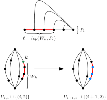
In Lemma 4.11, to compute the reachable nodes of knowing the reachable nodes of , fast matrix multiplication is employed (Lemma 4.10), but in this special case a simpler method will be more effective. For , let be the unique string read between nodes and in the path-graph of . The crucial observation is: the edges going out of node for end in nodes for , where as the strings from matching the prefix of are exactly all the prefixes of of length at most (see Figure 8).
Hence, to compute the reachable subset of , we can handle the edges going out of separately in time by letter comparisons, then compute the values for all the reachable nodes either using the LCP data structure, or with the use of the generalized suffix tree of in total time, and finally, using a 1D line sweep approach, compute the union of the obtained intervals in time. In the end, we answer YES if and only if node is reachable.
Over all values of this gives an algorithm running in total time. ∎
Furthermore, one may be allowed to choose, for each , a lower bound on the length of the prefix of used in the acronym (some strings should not be completely excluded from the acronym). The only modification to the algorithm in such a generalization is replacing intervals by , which does not influence the claimed complexity.
Corollary 5.2.
If the answer to the instance of the AG problem is YES, we can output all strings in which are acronyms of within time.
Proof.
We want to find out which strings of represent acronyms of . In the algorithm employed by Theorem 5.1 the reachable nodes of are found. If there exists an edge from a reachable node for to for some , then the path of the path-graph of containing node represents an acronym of . If node is reached directly from reachable node , then the whole prefix of used to do that is in , and hence is a standalone acronym of . If for a path neither of the two cases qualifies, then it cannot be used to reach node , and hence is not an acronym of . ∎
If the generalization with minimal lengths of prefixes is applied, then the values of used here are restricted to , where is the largest value of with a restriction : node does not have an edge to node , and hence does not belong to any path from to ).
Let us remark that although the main focus of real-world acronym generation systems is on the natural language parsing and interpretation of acronyms, our new algorithmic solution may inspire practical improvements in such systems or further algorithmic work.
6 ED String Comparison Tasks
In this section, we show some applications of our techniques from LABEL:{sec:EDSI}. In particular, we show how intersection graphs can be used to solve different ED string comparison tasks.
We consider two ED strings, of length , cardinality and size , and of length , cardinality and size . We call intersection graph the underlying graph of an automaton representing . By Corollary 4.5 such an automaton (and therefore the corresponding intersection graph) can be constructed in time. In Section 4, such a graph was used to check whether is nonempty.
In the following, we present other applications of intersection graphs (computed by means of Corollary 4.5 or Lemma 4.7) to tackle several natural ED string comparison tasks with no additional time complexity. We always assume that and are over an integer alphabet .
6.1 Shortest/Longest Witness
Let us start with the most basic application.
EDSI Shortest/Longest Witness Input: Two ED strings, of length , cardinality and size , and of length , cardinality and size . Output: A shortest (resp. longest) element of if it is a nonempty set, FAIL otherwise.
Fact 6.1.
The EDSI Shortest/Longest Witness problem can be solved in time by using an intersection graph of and .
Proof.
We compute the intersection graph as the underlying graph of the automaton computed in Corollary 4.5. Given an edge in , we assign a weight equal to the length of its string label (the string has length ). Note that, by construction, is a directed acyclic graph (DAG). Thus the problem reduces to computing the shortest or the longest path between a source and a sink of a DAG, a problem with a well-known linear-time solution that involves topological sorting. By reading the labels on the shortest (resp. longest) path in time, we can output the shortest (resp. longest) element of .444In the case of a shortest witness, we can obtain an equally efficient algorithm by employing Dijkstra’s algorithm using bucket queue since the bound on the weight of the path is known beforehand. ∎
6.2 Counting Pairs of Matching Strings
In the next task, we would like to compute the total number of matching pairs of strings in considering multiplicities in and . We assume that the multiplicity of a string in is the number of sequences such that . The definition for is analogous.
EDSI Matching Pairs Count Input: Two ED strings, of length , cardinality and size , and of length , cardinality and size . Output: .
Each matching pair can be represented by a pair of alignments: the sequence of choices of a single production and for each and , such that the resulting standard string is the same. Such a pair of alignments can in turn be represented by a path in the intersection graph of and as the edges correspond to (parts of) productions in some and in some .
The representation is almost unique; the only reason this does not need to be the case is when a node is reached from a node for using only -edges. In this case, the three subpaths and , all correspond to the choice of productions and , even though this choice should be counted as one.
To fix the notation, we call an -edge: vertical, when it leads from a node to for some explicit node of ; horizontal, when it leads from a node to for some explicit node of ; and diagonal if it leads from a node to , where both and are explicit nodes.
The problem becomes even more complicated when a few such -productions are used in a row in both ED strings (a node is reached from using only -edges), as a single alignment would correspond to all the “down, right or diagonal” paths in the grid. The number of such paths can be large, and even if we remove all such diagonal -edges (those can be always simulated with a single horizontal and a single vertical one), we cannot remove the horizontal or vertical ones, as those can be traversed by other paths independently. We are still left with equivalent subpaths from to . In order to mitigate this problem we will restrict the usage of such subpaths of many -edges to a single, regular one.
We call a path -regular, if it does not use diagonal -edges, and if two -edges are used sequentially, then they either have the same direction, or the second one is horizontal.
Lemma 6.2.
There is a one-to-one correspondence between pairs of alignments that produce the same string and -regular paths from the starting to the accepting node in the intersection graph of and .
Proof.
Consider a pair of alignments; it can be represented by the produced string together with some positions in-between letters marked with -labels and -labels in total specifying the beginning and ending of the productions used in and , for . A single position can be marked with both types of label and even many labels of the same type (when -productions are used). Each position corresponds to a pair of states in the path-automata: those pairs of states with at least one label read from left to right form a path in the intersection graph, as the -label shows that the state is explicit in . If two labels of a different type appear in the same place, this corresponds to a node composed of two explicit states. When a single position contains multiple labels from both types, the exact ordering between those labels represents the actual path in the graph. At the same time from the point of view of and separately all those orderings correspond to exactly the same pair of alignments. This is where -regularity plays its role and only one subpath is created (all -labels are placed before the -labels). This way we have defined an injection from the pairs of alignments to the paths of the intersection graph (each pair of alignments corresponds to only one -regular path).
On the other hand the labels of the edges in the path represent (the parts of) the transitions used in each automaton, and hence also a pair of alignments, thus the function is also surjective.
We have thus shown that the function relating a pair of alignments to a path is both injective and surjective, and hence a bijection (the one-to-one correspondence from the statement). ∎
The main result then follows.
Fact 6.3.
The EDSI Matching Pairs Count problem can be solved in time by using an intersection graph of and .
Proof.
We compute the intersection graph as the underlying graph of the automaton computed in Corollary 4.5 or Lemma 4.7. By Lemma 6.2, we are counting distinct -regular paths from the starting node to the accepting one. As previously, we can sort the nodes topologically. If we wanted to count all the paths it would be enough to compute for each node the value equal to the number of paths from the starting node to . One would have , over all edges (including parallel edges with different labels) and setting where is the starting node. This time, however, we apply slightly more complicated formulas, which count the paths ending with the -edges separately from the other ones, and among those separately depending on the direction of the -edge. For a node , let , and denote the number of -regular paths from the starting node to the node that end with an edge with a non-empty label, with a horizontal -edge and with a vertical -edge, respectively.
-
•
-
•
-
•
By induction, for the accepting node , the number of distinct -regular paths from the starting to the accepting node is equal to the sum of the values , and computed for node . ∎
6.3 ED Matching Statistics
Asking whether is not nonempty, as a way to tell if two ED strings have something in common, can be too restrictive in practical applications. We will thus consider two more elaborate ED string comparison tasks that consider local matches rather than a match that necessarily involves the entire ED strings from beginning to end. Both notions that we consider, Matching Statistics and Longest Common Substring, are heavily employed on standard strings for practical applications, especially in bioinformatics.
We start by extending the classic Matching Statistics problem [37] from the standard string setting to the ED string setting. Although this solution has already been described in [32], we provide it also here as an intermediate step of the solution to the next comparison task.
ED Matching Statistics Input: Two ED strings, of length , cardinality and size , and of length , cardinality and size . Output: For each , the length of the longest prefix of a string in that is a substring of a string in .
Fact 6.4.
The ED Matching Statistics problem can be solved in time by using an intersection graph of and .
Proof.
This time we will use a slightly augmented version of the intersection graph coming from the unpruned intersection automaton. Namely, we construct the automaton as in Corollary 4.5, but do not remove the unreachable parts or the “partial transitions”. That is, when we process an explicit state corresponding to a pair of states in the path-automata and , and a pair of transitions going out of and , we construct the corresponding transition to the pair of states that can be reached through and , even if this transition finishes in a pair of implicit states, namely when , where and are the respective labels of and . Even in that case, the number of transition pair checks remains the same, and therefore the total size of the constructed underlying graph stays .
Once again we assign to each edge the weight storing the length of its string label and process the nodes in the reversed topological order to compute for each node the value equal to the length of the longest path from in that matches a path in ; we have where iterates over all successors of . One has for the nodes that do not have successors (for example the accepting node or nodes corresponding to a pair of implicit states).
By construction, we have , for an explicit state of and a state of , if and only if is equal to the maximal LCP between a pair , where a string in and is a string read starting at (explicit or implicit) state in .
For every explicit state of we can compute over all (explicit or implicit) states of to obtain the output. ∎
An example of this construction is shown in Figure 9.

6.4 ED Longest Common Substring
We now proceed to extending the classic Longest Common Substring problem [37] from the standard string setting to the ED string setting.
ED Longest Common Substring Input: Two ED strings, of length , cardinality and size , and of length , cardinality and size . Output: A longest string that occurs in a string of and a string of
In the ED Matching Statistics problem only strings starting in explicit nodes of were considered; here we want to lift this restriction. Computing the value of for every node of against every node of would take time. We are only interested in the globally maximal value of . Hence, we can focus only on the computation of those values for a certain subset of those pairs.
Fact 6.5.
The ED Longest Common Substring problem can be solved in time by using an intersection graph of and .
Proof.
We start from the augmented graph , as defined in the proof of 6.4, and computed in time. In addition to the standard edges between the explicit nodes, the graph contains edges from a pair containing at least one explicit state to a pair of implicit states, that are inclusion-wise maximal, that is, cannot be extended to obtain a longer edge. For the ED Longest Common Substring problem, we additionally need edges symmetric to those – the (inclusion-wise maximal) edges starting in pairs of implicit states that end in pairs containing at least one explicit state. By a symmetric argument (argument for the reversed automata), there are such edges and all can be computed together with the rest of the graph within the same time complexity. We compute the values for each node as previously, and find their global maximum. Notice that if for an implicit node associates with another implicit node , we do not need to compute the value . Indeed, then lies in the middle of an edge and the first node of its predecessor on the edge always has a greater value of .
We are left with the nodes that are not (weakly) connected to any explicit node. The isolated edges containing such nodes were not computed at all. Those edges correspond to strings that, in both ED strings, are fully contained in a single set. Hence, it is enough to compute the longest common substring of two strings, one being a concatenation of strings in and the other a concatenation of strings in , for sentinel letters #, $. This can be done in time.
The method of obtaining the witness is the same as in the previous problems (after computing both endpoints of the optimal path using the algorithm described above). ∎
6.5 ED Longest Common Subsequence
Finally, we show how to extend the classic Longest Common Subsequence (LCS) problem [37] from the standard string setting to the ED string setting. We remark that, unlike the previous problems, in the standard string setting, LCS is not solvable in linear time: there exists a conditional lower bound saying that no algorithm with running time , for any , can solve LCS on two length- strings unless SETH fails [18].
ED Longest Common Subsequence Input: Two ED strings, of size , and of size . Output: A longest string that occurs in a string of and a string of as a subsequence.
Fact 6.6.
The ED Longest Common Subsequence problem can be solved in time by using an uncompacted intersection graph of and .
Proof.
Consider the uncompacted path-automata for and , having respective sizes , . For every single transition in those graphs (that is a single letter transition since they are uncompacted), we add a parallel -transition (that is, we allow to skip the letter). The sizes of the automata remain and , and the intersection has size . We can then find the longest witness (6.1) of this intersection in time linear in the size of the automaton, that is, in time. ∎
Notice that when and are standard strings, then and running time matches the conditional lower bound for standard strings up to subpolynomial factors. Hence, no can be replaced by or . In particular, an time algorithm would refute the conditional lower bound.
Proposition 6.7.
In all the solutions presented in this section (as well as in the previous ones) the algorithm can be slightly modified to achieve space complexity without any increase in the running time.
Proof.
Notice that all the problems are solved through computing a certain value (reachability, ) for all the explicit nodes of the intersection graph in a topological order. Each time this order is compatible with the order of sets of and , and the recurrent formulas refer only to nodes from a single set or , that is, the basic computation is enclosed in a single cell of the grid (inspect Fig. 6(a)). For a single cell of the grid the space used for computation is , while globally the information passed between the cells is bounded by by going through the cells in a lexicographical (or reversed lexicographical) order (it is enough to store information for nodes of only for the next two values of ). Finally the size of the input as well as of all the generalized suffix trees is also bounded by . ∎
7 (Doubly) Elastic-Degenerate String Matching
String matching (or pattern matching) on standard strings can be seen as a natural (and very useful) generalization of string equality. Since EDSI is basically a counterpart of the string equality problem (we seek for a pair of standard strings from and from that are equal), the problem of generalizing it to string matching arises naturally [39]. In particular, the ED String Matching (EDSM) problem of locating the occurrences of a pattern that is a standard string in an ED text has already been considered [4, 14, 15, 36, 39].
For a standard string and an ED text , one wants to check whether occurs in , that is, if it is a substring of some string (decision version), or find all the segments of such that an occurrence of starts within a string of the set ; i.e., there exists a standard string with an alignment such that occurs in starting at a position lying in the th segment of the alignment.
In this section, we consider the EDSM problem in its full generality, i.e., both the text and the pattern are ED strings. We then show how our solution instantiates to the special cases, where one of the two ED strings is a standard string.
Let us now define the general problem in scope:
Doubly ED String Matching Input: An ED string (called text) and an ED string (called pattern). Output: YES if and only if there is a string that is a substring of a string (decision version); or all segments such that there is a string whose occurrence in starts in (reporting version).
Through applying the solution to reversed ED strings and (we reverse the sequence of segments and the strings inside them), we can see that the reporting version can be used to find all the segments where an occurrence ends. Further note that Doubly ED String Matching is equivalent to asking for the union of the results of EDSM over all the patterns from – we take a binary OR of the results for the decision version.
The algorithms underlying Theorem 4.6 and Theorem 4.12 can both be extended to solve Doubly ED String Matching:
Theorem 7.1.
We can solve the reporting or decision version of Doubly ED String Matching on an ED text having length , cardinality and size , and an ED pattern having length , cardinality and size in time or in time.
Proof.
Like in EDSI, we need to check whether an accepting state is reachable from a starting one, on the very same intersection graph. This time, however, for every state of the path-automaton of , we make every node reachable (starting), and every node accepting. That way, after computing every reachable node with one of the algorithms underlying Theorem 4.6 or Theorem 4.12, an accepting node is reachable if and only if a string in occurs at any position of a string from . The complexity is the same as before, since the size of graph remains unchanged.
For the reporting version, we observe that occurrences ending in set correspond to reachable nodes in the set . Hence, we simply report the list of such sets containing a reachable node, which can be done in total time over all . The starting positions can be reported through the use of reversed strings. ∎
In [5, Corollary 10] it was shown that Doubly ED String Matching cannot be solved in time or time, for any constant , unless the OV conjecture is false. This result does not contradict our result as the lengths can in general be large.
Notice that if the pattern is a standard string () the transitions from to are there solely to check if occurs in any string from (which can be done in time). Hence, similarly to Corollary 4.13 the running time of our FMM algorithm is equal to . This complexity (and design) matches the result of [15].
Symmetrically, if the text is a standard string (), then the FMM solution runs in time (this time like in case of Corollary 4.13 the edges from to are not considered at all).
8 Approximate EDSI
Another popular extension of string equality is approximate equality, where one wants to find the distance between two strings: the minimal number of operations that modify one string into the other one, or decide whether this number is at most , for a given integer .
We denote by (resp. ) the Hamming distance (resp. edit distance) of two standard strings . The problem of finding the Hamming distance of two standard strings is easily solvable in time, while for edit distance the time increases to time in general case [61] or [48] for a given upper bound .
Approximate EDSI gives another measure of similarity when the normal intersection turns out to be empty.
Theorem 8.1.
Given a pair of ED strings of sizes and , respectively, we can find the pair minimizing the distance or in time.
Proof.
We adapt the classic Wagner–Fischer algorithm [61] to our case. We construct the standard (uncompacted) NFA intersection of the two path-automata for and , set the weight of all its edges to , and then add extra edges with weight that represent edit operations.
In case of Hamming distance, when a pair of transitions , does not match () we still add the weight- edge between and ( is substituted with ).
In case of edit distance we additionally construct weight- edges from to for every transition (corresponding to deletion of the letter ), and to for every transition (corresponding to insertion of letter ).
Now all we need to do is to find the minimum cost path from the starting node to the accepting one (in case of Hamming distance only if such a path exists), which can be done in linear time using Dial’s implementation of Dijkstra’s algorithm [24]. By simply spelling the labels of the found path we obtain strings and (the difference between them is encoded through the labels of the weight- edges). ∎
Without having a threshold , even when are standard strings (), for the edit distance we cannot obtain an algorithm running in time for a constant unless SETH fails [9], or a faster algorithm through a parameterization with .
On the other hand, if we are given a threshold , we can adapt another classic algorithm, given by Landau and Vishkin [49], to obtain the following theorem.
Theorem 8.2.
Given an ED string of cardinality and size , an ED string of cardinality and size , and an integer , we can check whether a pair with (resp. ) exists in time (resp. in time) and, if that is the case, return the pair with the smallest distance.
Proof.
This time we make use of the compacted intersection automaton from Lemma 4.3. In addition to standard weight- edges, which are constructed when for being the labels of extended transitions in the two path-automata, we also add new edges when one of the strings is at distance at most from a prefix of the other one. More formally, for a pair of extended transitions , , if is at distance from the length- prefix of , we produce a weight- edge from to , where is the implicit state between and representing the length prefix of (symmetrically for at distance at most from a prefix of ). All such values of can be found with the use of a standard LCP queries data structure and kangaroo jumps [33] in time for Hamming distance and in time for edit distance [49].
In case of Hamming distance, the total number of extended transitions is still (the number of transition checks does not change). In case of edit distance, it can increase by a factor of . Indeed, for a single pair of transitions , we can produce up to weighted transitions.
After that, once again, we can use Dial’s implementation of Dijkstra’s algorithm [24] to find the smallest weight path in this graph, obtaining the claimed result. ∎
One may notice that the modifications to the standard intersection algorithms from this section and the previous one are independent; in the previous section those consisted of marking additional nodes as starting/accepting, while in this section those consisted of adding edges. By applying both modifications simultaneously, we can solve the Approximate (Doubly) EDSM problem, that is, the problem of finding a pair of strings such that is at distance at most from a substring of (for which this distance is minimized). We thus obtain the following result:
Corollary 8.3.
Approximate (Doubly) EDSM can be solved in time in general, or in time for Hamming distance and time for edit distance when we are given an integer as an upper bound on the sought distance.
Once again we can notice that when pattern is a standard string this time complexity can be bounded by a smaller value – we can check if the pattern appears in any of the strings from any of the sets in total time [49]. Otherwise each edge used has at least one endpoint in a node , where is an explicit state from the automaton representing , hence the total number edge checks in this case is equal to (we can compute the backwards edges the same way as the forward ones), thus we obtain the total running time of for Hamming distance and time for edit distance. Our results match the time complexity of the corresponding results of [16]. (Note that [16] uses to denote and to denote .)
Symmetrically, when text is a standard string those time complexities are and , respectively, since in this case every useful edge has at least one endpoint in a node , where is an explicit state from the automaton representing .
9 Open Questions
In our view, the main open questions that stem from our work are as follows.
-
•
We showed an -time algorithm for EDSI. Can one design an -time (perhaps not combinatorial) algorithm for EDSI, for some ?
-
•
We showed that there is no combinatorial -time algorithm for EDSI. Can one show a stronger conditional lower bound for combinatorial algorithms?
-
•
We showed an -time algorithm for outputting a representation of the intersection language of two unary ED strings. Can one design an -time algorithm?
References
- [1] Amir Abboud and Virginia Vassilevska Williams. Popular conjectures imply strong lower bounds for dynamic problems. In 55th IEEE Annual Symposium on Foundations of Computer Science, FOCS 2014, Philadelphia, PA, USA, October 18-21, 2014, pages 434–443. IEEE Computer Society, 2014.
- [2] Mai Alzamel, Lorraine A. K. Ayad, Giulia Bernardini, Roberto Grossi, Costas S. Iliopoulos, Nadia Pisanti, Solon P. Pissis, and Giovanna Rosone. Degenerate string comparison and applications. In Laxmi Parida and Esko Ukkonen, editors, 18th International Workshop on Algorithms in Bioinformatics, WABI 2018, August 20-22, 2018, Helsinki, Finland, volume 113 of LIPIcs, pages 21:1–21:14. Schloss Dagstuhl - Leibniz-Zentrum für Informatik, 2018.
- [3] Mai Alzamel, Lorraine A. K. Ayad, Giulia Bernardini, Roberto Grossi, Costas S. Iliopoulos, Nadia Pisanti, Solon P. Pissis, and Giovanna Rosone. Comparing degenerate strings. Fundam. Inform., 175(1-4):41–58, 2020.
- [4] Kotaro Aoyama, Yuto Nakashima, Tomohiro I, Shunsuke Inenaga, Hideo Bannai, and Masayuki Takeda. Faster online elastic degenerate string matching. In Gonzalo Navarro, David Sankoff, and Binhai Zhu, editors, Annual Symposium on Combinatorial Pattern Matching, CPM 2018, July 2-4, 2018 - Qingdao, China, volume 105 of LIPIcs, pages 9:1–9:10. Schloss Dagstuhl - Leibniz-Zentrum für Informatik, 2018.
- [5] Rocco Ascone, Giulia Bernardini, Alessio Conte, Massimo Equi, Estéban Gabory, Roberto Grossi, and Nadia Pisanti. A unifying taxonomy of pattern matching in degenerate strings and founder graphs. In Solon P. Pissis and Wing-Kin Sung, editors, 24th International Workshop on Algorithms in Bioinformatics, WABI 2024, September 2-4, 2024, Royal Holloway, London, United Kingdom, volume 312 of LIPIcs, pages 14:1–14:21. Schloss Dagstuhl - Leibniz-Zentrum für Informatik, 2024.
- [6] Lorraine A. K. Ayad, Carl Barton, and Solon P. Pissis. A faster and more accurate heuristic for cyclic edit distance computation. Pattern Recognit. Lett., 88:81–87, 2017.
- [7] Jasmijn A. Baaijens, Paola Bonizzoni, Christina Boucher, Gianluca Della Vedova, Yuri Pirola, Raffaella Rizzi, and Jouni Sirén. Computational graph pangenomics: a tutorial on data structures and their applications. Nat. Comput., 21(1):81–108, 2022.
- [8] Arturs Backurs and Piotr Indyk. Which regular expression patterns are hard to match? In Irit Dinur, editor, IEEE 57th Annual Symposium on Foundations of Computer Science, FOCS 2016, 9-11 October 2016, Hyatt Regency, New Brunswick, New Jersey, USA, pages 457–466. IEEE Computer Society, 2016.
- [9] Arturs Backurs and Piotr Indyk. Edit distance cannot be computed in strongly subquadratic time (unless SETH is false). SIAM J. Comput., 47(3):1087–1097, 2018.
- [10] Ricardo Baeza-Yates and Berthier A. Ribeiro-Neto. Modern Information Retrieval - the concepts and technology behind search, Second edition. Pearson Education Ltd., Harlow, England, 2011.
- [11] Michael A. Bender and Martin Farach-Colton. The LCA problem revisited. In Gaston H. Gonnet, Daniel Panario, and Alfredo Viola, editors, LATIN 2000: Theoretical Informatics, 4th Latin American Symposium, Punta del Este, Uruguay, April 10-14, 2000, Proceedings, volume 1776 of Lecture Notes in Computer Science, pages 88–94. Springer, 2000.
- [12] Giulia Bernardini, Alessio Conte, Garance Gourdel, Roberto Grossi, Grigorios Loukides, Nadia Pisanti, Solon P. Pissis, Giulia Punzi, Leen Stougie, and Michelle Sweering. Hide and mine in strings: Hardness and algorithms. In Claudia Plant, Haixun Wang, Alfredo Cuzzocrea, Carlo Zaniolo, and Xindong Wu, editors, 20th IEEE International Conference on Data Mining, ICDM 2020, Sorrento, Italy, November 17-20, 2020, pages 924–929. IEEE, 2020.
- [13] Giulia Bernardini, Estéban Gabory, Solon P. Pissis, Leen Stougie, Michelle Sweering, and Wiktor Zuba. Elastic-degenerate string matching with 1 error. In Armando Castañeda and Francisco Rodríguez-Henríquez, editors, LATIN 2022: Theoretical Informatics - 15th Latin American Symposium, Guanajuato, Mexico, November 7-11, 2022, Proceedings, volume 13568 of Lecture Notes in Computer Science, pages 20–37. Springer, 2022.
- [14] Giulia Bernardini, Paweł Gawrychowski, Nadia Pisanti, Solon P. Pissis, and Giovanna Rosone. Even faster elastic-degenerate string matching via fast matrix multiplication. In Christel Baier, Ioannis Chatzigiannakis, Paola Flocchini, and Stefano Leonardi, editors, 46th International Colloquium on Automata, Languages, and Programming, ICALP 2019, July 9-12, 2019, Patras, Greece, volume 132 of LIPIcs, pages 21:1–21:15. Schloss Dagstuhl - Leibniz-Zentrum für Informatik, 2019.
- [15] Giulia Bernardini, Paweł Gawrychowski, Nadia Pisanti, Solon P. Pissis, and Giovanna Rosone. Elastic-degenerate string matching via fast matrix multiplication. SIAM J. Comput., 51(3):549–576, 2022.
- [16] Giulia Bernardini, Nadia Pisanti, Solon P. Pissis, and Giovanna Rosone. Approximate pattern matching on elastic-degenerate text. Theor. Comput. Sci., 812:109–122, 2020.
- [17] Philip Bille and Inge Li Gørtz. Sparse regular expression matching. In David P. Woodruff, editor, Proceedings of the 2024 ACM-SIAM Symposium on Discrete Algorithms, SODA 2024, Alexandria, VA, USA, January 7-10, 2024, pages 3354–3375. SIAM, 2024.
- [18] Karl Bringmann and Marvin Künnemann. Quadratic conditional lower bounds for string problems and dynamic time warping, 2015.
- [19] Chris Calabro, Russell Impagliazzo, and Ramamohan Paturi. The complexity of satisfiability of small depth circuits. In Jianer Chen and Fedor V. Fomin, editors, Parameterized and Exact Computation, 4th International Workshop, IWPEC 2009, Copenhagen, Denmark, September 10-11, 2009, Revised Selected Papers, volume 5917 of Lecture Notes in Computer Science, pages 75–85. Springer, 2009.
- [20] Vincenzo Carletti, Pasquale Foggia, Erik Garrison, Luca Greco, Pierluigi Ritrovato, and Mario Vento. Graph-based representations for supporting genome data analysis and visualization: Opportunities and challenges. In Donatello Conte, Jean-Yves Ramel, and Pasquale Foggia, editors, Graph-Based Representations in Pattern Recognition - 12th IAPR-TC-15 International Workshop, GbRPR 2019, Tours, France, June 19-21, 2019, Proceedings, volume 11510 of Lecture Notes in Computer Science, pages 237–246. Springer, 2019.
- [21] Aleksander Cisłak, Szymon Grabowski, and Jan Holub. SOPanG: online text searching over a pan-genome. Bioinform., 34(24):4290–4292, 2018.
- [22] Thomas H. Cormen, Charles E. Leiserson, Ronald L. Rivest, and Clifford Stein. Introduction to Algorithms, 3rd Edition. MIT Press, 2009.
- [23] Maxime Crochemore, Christophe Hancart, and Thierry Lecroq. Algorithms on Strings. Cambridge University Press, 2007.
- [24] Robert B. Dial. Algorithm 360: shortest-path forest with topological ordering [H]. Commun. ACM, 12(11):632–633, 1969.
- [25] N. Rex Dixon and Thomas B. Martin. Automatic Speech and Speaker Recognition. John Wiley & Sons, Inc., USA, 1979.
- [26] Esteban Domingo, Carlos García-Crespo, and Celia Perales. Historical perspective on the discovery of the quasispecies concept. Annu. Rev. Virol., 8(1):51–72, 2021. PMID: 34586874.
- [27] Massimo Equi, Veli Mäkinen, Alexandru I. Tomescu, and Roberto Grossi. On the complexity of string matching for graphs. ACM Trans. Algorithms, 19(3):21:1–21:25, 2023.
- [28] Massimo Equi, Tuukka Norri, Jarno Alanko, Bastien Cazaux, Alexandru I. Tomescu, and Veli Mäkinen. Algorithms and complexity on indexing founder graphs. Algorithmica, 85(6):1586–1623, 2023.
- [29] Martin Farach. Optimal suffix tree construction with large alphabets. In 38th Annual Symposium on Foundations of Computer Science, FOCS 1997, Miami Beach, Florida, USA, October 19-22, 1997, pages 137–143. IEEE Computer Society, 1997.
- [30] Michael L. Fredman, János Komlós, and Endre Szemerédi. Storing a sparse table with O(1) worst case access time. J. ACM, 31(3):538–544, 1984.
- [31] Estéban Gabory, Njagi Moses Mwaniki, Nadia Pisanti, Solon P. Pissis, Jakub Radoszewski, Michelle Sweering, and Wiktor Zuba. Comparing elastic-degenerate strings: Algorithms, lower bounds, and applications. In Laurent Bulteau and Zsuzsanna Lipták, editors, 34th Annual Symposium on Combinatorial Pattern Matching, CPM 2023, June 26-28, 2023, Marne-la-Vallée, France, volume 259 of LIPIcs, pages 11:1–11:20. Schloss Dagstuhl - Leibniz-Zentrum für Informatik, 2023.
- [32] Estéban Gabory, Njagi Moses Mwaniki, Nadia Pisanti, Solon P. Pissis, Jakub Radoszewski, Michelle Sweering, and Wiktor Zuba. Pangenome comparison via ED strings. Frontiers Bioinform., 2024. Under Review.
- [33] Zvi Galil and Raffaele Giancarlo. Improved string matching with k mismatches. SIGACT News, 17(4):52–54, mar 1986.
- [34] Paweł Gawrychowski, Samah Ghazawi, and Gad M. Landau. On indeterminate strings matching. In Inge Li Gørtz and Oren Weimann, editors, 31st Annual Symposium on Combinatorial Pattern Matching, CPM 2020, June 17-19, 2020, Copenhagen, Denmark, volume 161 of LIPIcs, pages 14:1–14:14. Schloss Dagstuhl - Leibniz-Zentrum für Informatik, 2020.
- [35] Daniel Gibney. An efficient elastic-degenerate text index? Not likely. In Christina Boucher and Sharma V. Thankachan, editors, String Processing and Information Retrieval - 27th International Symposium, SPIRE 2020, Orlando, FL, USA, October 13-15, 2020, Proceedings, volume 12303 of Lecture Notes in Computer Science, pages 76–88. Springer, 2020.
- [36] Roberto Grossi, Costas S. Iliopoulos, Chang Liu, Nadia Pisanti, Solon P. Pissis, Ahmad Retha, Giovanna Rosone, Fatima Vayani, and Luca Versari. On-line pattern matching on similar texts. In Juha Kärkkäinen, Jakub Radoszewski, and Wojciech Rytter, editors, 28th Annual Symposium on Combinatorial Pattern Matching, CPM 2017, July 4-6, 2017, Warsaw, Poland, volume 78 of LIPIcs, pages 9:1–9:14. Schloss Dagstuhl - Leibniz-Zentrum für Informatik, 2017.
- [37] Dan Gusfield. Algorithms on Strings, Trees, and Sequences - Computer Science and Computational Biology. Cambridge University Press, 1997.
- [38] Paul Heckel. A technique for isolating differences between files. Commun. ACM, 21(4):264–268, 1978.
- [39] Costas S. Iliopoulos, Ritu Kundu, and Solon P. Pissis. Efficient pattern matching in elastic-degenerate strings. Inf. Comput., 279:104616, 2021.
- [40] Russell Impagliazzo and Ramamohan Paturi. On the complexity of k-SAT. J. Comput. Syst. Sci., 62(2):367–375, 2001.
- [41] Russell Impagliazzo, Ramamohan Paturi, and Francis Zane. Which problems have strongly exponential complexity? J. Comput. Syst. Sci., 63(4):512–530, 2001.
- [42] IUPAC-IUB Commission on Biochemical Nomenclature. Abbreviations and symbols for nucleic acids, polynucleotides, and their constituents. Biochemistry, 9(20):4022–4027, 1970.
- [43] Kayla Jacobs, Alon Itai, and Shuly Wintner. Acronyms: identification, expansion and disambiguation. Ann. Math. Artif. Intell., 88(5-6):517–532, 2020.
- [44] Katrin Kirchhoff and Anne M. Turner. Unsupervised resolution of acronyms and abbreviations in nursing notes using document-level context models. In Cyril Grouin, Thierry Hamon, Aurélie Névéol, and Pierre Zweigenbaum, editors, Proceedings of the Seventh International Workshop on Health Text Mining and Information Analysis, Louhi@EMNLP 2016, Austin, TX, USA, November 5, 2016, pages 52–60. Association for Computational Linguistics, 2016.
- [45] Jon M. Kleinberg and Éva Tardos. Algorithm Design. Addison-Wesley, 2006.
- [46] Divesh R. Kubal and Apurva Nagvenkar. Effective ensembling of transformer based language models for acronyms identification. In Amir Pouran Ben Veyseh, Franck Dernoncourt, Thien Huu Nguyen, Walter Chang, and Leo Anthony Celi, editors, Proceedings of the Workshop on Scientific Document Understanding co-located with 35th AAAI Conference on Artificial Inteligence, SDU@AAAI 2021, Virtual Event, February 9, 2021, volume 2831 of CEUR Workshop Proceedings. CEUR-WS.org, 2021.
- [47] Cheng-Ju Kuo, Maurice H. T. Ling, Kuan-Ting Lin, and Chun-Nan Hsu. BIOADI: a machine learning approach to identifying abbreviations and definitions in biological literature. BMC Bioinform., 10(S-15):7, 2009.
- [48] Gad M. Landau, Eugene W. Myers, and Jeanette P. Schmidt. Incremental string comparison. SIAM J. Comput., 27(2):557–582, 1998.
- [49] Gad M Landau, Uzi Vishkin, and Ruth Nussinov. An efficient string matching algorithm with k differences for nucleotide and amino acid sequences. Nucleic Acids Res., 14(1):31–46, 1986.
- [50] Mark V. Lawson. Finite Automata. Chapman and Hall/CRC, 2004.
- [51] Jie Liu, Caihua Liu, and Yalou Huang. Multi-granularity sequence labeling model for acronym expansion identification. Inf. Sci., 378:462–474, 2017.
- [52] Veli Mäkinen, Bastien Cazaux, Massimo Equi, Tuukka Norri, and Alexandru I. Tomescu. Linear time construction of indexable founder block graphs. In Carl Kingsford and Nadia Pisanti, editors, 20th International Workshop on Algorithms in Bioinformatics, WABI 2020, September 7-9, 2020, Pisa, Italy (Virtual Conference), volume 172 of LIPIcs, pages 7:1–7:18. Schloss Dagstuhl - Leibniz-Zentrum für Informatik, 2020.
- [53] Udi Manber and Sun Wu. An algorithm for approximate membership checking with application to password security. Inf. Process. Lett., 50(4):191–197, 1994.
- [54] Gonzalo Navarro. A guided tour to approximate string matching. ACM Comput. Surv., 33(1):31–88, 2001.
- [55] Nicola Rizzo, Massimo Equi, Tuukka Norri, and Veli Mäkinen. Elastic founder graphs improved and enhanced. Theor. Comput. Sci., 982:114269, 2024.
- [56] Ariel S. Schwartz and Marti A. Hearst. A simple algorithm for identifying abbreviation definitions in biomedical text. In Russ B. Altman, A. Keith Dunker, Lawrence Hunter, and Teri E. Klein, editors, Proceedings of the 8th Pacific Symposium on Biocomputing, PSB 2003, Lihue, Hawaii, USA, January 3-7, 2003, pages 451–462, 2003.
- [57] Kazem Taghva and Jeff Gilbreth. Recognizing acronyms and their definitions. Int. J. Document Anal. Recognit., 1(4):191–198, 1999.
- [58] The Computational Pan-Genomics Consortium. Computational pan-genomics: status, promises and challenges. Briefings Bioinform., 19(1):118–135, 2018.
- [59] Virginia Vassilevska Williams and Ryan Williams. Subcubic equivalences between path, matrix and triangle problems. In 51th Annual IEEE Symposium on Foundations of Computer Science, FOCS 2010, October 23-26, 2010, Las Vegas, Nevada, USA, pages 645–654. IEEE Computer Society, 2010.
- [60] Amir Pouran Ben Veyseh, Franck Dernoncourt, Quan Hung Tran, and Thien Huu Nguyen. What does this acronym mean? Introducing a new dataset for acronym identification and disambiguation. In Donia Scott, Núria Bel, and Chengqing Zong, editors, Proceedings of the 28th International Conference on Computational Linguistics, COLING 2020, Barcelona, Spain (Online), December 8-13, 2020, pages 3285–3301. International Committee on Computational Linguistics, 2020.
- [61] Robert A. Wagner and Michael J. Fischer. The string-to-string correction problem. J. ACM, 21(1):168–173, 1974.
- [62] Ryan Williams. A new algorithm for optimal 2-constraint satisfaction and its implications. Theor. Comput. Sci., 348(2-3):357–365, 2005.