Topological resilience of optical skyrmions in local decoherence
Li-Wen Wang
CAS Key Laboratory of Quantum Information, University of Science and Technology of China, Hefei, 230026, China
CAS Center for Excellence in Quantum Information and Quantum Physics, University of Science and Technology of China, Hefei, 230026, China
Sheng Liu
shengliu@ustc.edu.cnCAS Key Laboratory of Quantum Information, University of Science and Technology of China, Hefei, 230026, China
CAS Center for Excellence in Quantum Information and Quantum Physics, University of Science and Technology of China, Hefei, 230026, China
Cheng-Jie Zhang
School of Physical Science and Technology, Ningbo University, Ningbo, 315211, China
Hefei National Laboratory, University of Science and Technology of China, Hefei, 230088, China
Geng Chen
CAS Key Laboratory of Quantum Information, University of Science and Technology of China, Hefei, 230026, China
CAS Center for Excellence in Quantum Information and Quantum Physics, University of Science and Technology of China, Hefei, 230026, China
Hefei National Laboratory, University of Science and Technology of China, Hefei, 230088, China
Yong-Sheng Zhang
yshzhang@ustc.edu.cnCAS Key Laboratory of Quantum Information, University of Science and Technology of China, Hefei, 230026, China
CAS Center for Excellence in Quantum Information and Quantum Physics, University of Science and Technology of China, Hefei, 230026, China
Hefei National Laboratory, University of Science and Technology of China, Hefei, 230088, China
Chuan-Feng Li
CAS Key Laboratory of Quantum Information, University of Science and Technology of China, Hefei, 230026, China
CAS Center for Excellence in Quantum Information and Quantum Physics, University of Science and Technology of China, Hefei, 230026, China
Hefei National Laboratory, University of Science and Technology of China, Hefei, 230088, China
Guang-Can Guo
CAS Key Laboratory of Quantum Information, University of Science and Technology of China, Hefei, 230026, China
CAS Center for Excellence in Quantum Information and Quantum Physics, University of Science and Technology of China, Hefei, 230026, China
Hefei National Laboratory, University of Science and Technology of China, Hefei, 230088, China
Abstract
The concept of skyrmions was introduced as early as the 1960s by Tony Skyrme. The topologically protected configuration embedded in skyrmions has prompted some investigations into their fundamental properties and versatile applications, sparking interest and guiding ongoing development. The topological protection associated with skyrmions was initially observed in systems with interactions. It is widely believed that skyrmions are stable yet relevant confirmation and empirical research remains limited. A pertinent question is whether skyrmion configurations formed by single-particle wave functions also exhibit topological stability. In this study, we affirm this hypothesis by investigating the effects of local decoherence. We analytically and numerically demonstrate the topological resilience of skyrmions and occurrence of transition points of skyrmion numbers in local decoherence of three typical decoherence channels. On the other hand, we show that these qualities are independent of the initial state. From the numerical results, we verify that inhomogeneous but continuous decoherence channels also adhere to the same behaviors and hold topological stability of skyrmions as homogeneous decoherence channels. These properties of skyrmions contribute to further applications in various areas including communication and imaging.
Introduction.—In the 1960s, Tony Skyrme introduced the concept of skyrmions primarily to describe the structure of nucleons Skyrme and Schonland (1961); Skyrme (1962). The skyrmion model proposes that nucleons are topological structures embedded in space, providing a theoretical framework to elucidate their interactions and dynamic behaviors. Thanks to their topological excitation properties, skyrmions find wide-ranging applications in fields such as condensed matter physics Bogdanov and Panagopoulos (2020); Wang et al. (2010), liquid crystals Nagase et al. (2019), and quantum Hall systems Taguchi et al. (2001); Neubauer et al. (2009); Pfleiderer and Rosch (2010); Ritz et al. (2013); Mochizuki et al. (2014). Not surprisingly, skyrmions textures can emerge in different physical systems with various mechanisms. Numerous researchers have delved into theoretical studies of magnetic skyrmions in magnetic systems and have experimentally observed their spin configurations Fert et al. (2017); Zhang et al. (2020) with some distinctive material environments, i.e. non-centrosymmetric ferromagnets Bogdanov and Yablonskii (1989); Bogdanov and Hubert (1994); Roessler et al. (2006); Mühlbauer et al. (2009); Yu et al. (2010) or centrosymmetric ferromagnets combined with uniaxial anisotropy Garel and Doniach (1982); Malozemoff and Slonczewski (2013) and even interface of ferromagnetic monolayers Heinze et al. (2011); Romming et al. (2013).
Given the potential and significant application prospects exhibited by skyrmions, counterpart in optics is now being developed to explore analogous topological properties Shen et al. (2024a) and it has been first realized by an evanescent electromagnetic field on an interface Tsesses et al. (2018); Du et al. (2019). Very recently, optical skyrmionic structures in free space based on vectorial optical fields having broad utilizations can be generated and observed by a superposition of two structured light modes Rosales-Guzmán et al. (2018); Wan et al. (2023); Nape et al. (2022); Peters et al. (2023) with two mutually orthogonal polarizations He et al. (2022); Gao et al. (2020); Gutiérrez-Cuevas and Pisanty (2021); Shen et al. (2022). Meanwhile, more advanced and sophisticated skyrmionic spin textures are revealed, such as various types of skyrmions named bimerons and merons Shen et al. (2024a); Lei et al. (2021); Jani et al. (2021), momentum space skyrmions Guo et al. (2020), space-time skyrmions with toroidal pulses Zdagkas et al. (2022); Shen et al. (2024b); Wang et al. (2024a, b) and even 3-dimensional (3D) hopfions Shen et al. (2023).
Skyrmions have topological protected configurations and can be characterized by the corresponding topological numbers, i.e. skyrmion numbers. It is commonly believed that skyrmions are stable. Therefore, skyrmions have huge application prospects in many fields and are becoming the focus of attention due to the topological stability. A few researchers have begun to do some investigations about the robustness of skyrmions against perturbations. Liu et al. investigated the robustness of optical skyrmions against disorder from random fluctuations in amplitude and phase of the field Liu et al. (2022). Ornelas et al. demonstrated experimentally the topological resilience of optical skyrmions to entanglement decay by an amplitude damping operation Ornelas et al. (2024). However, the empirical research in this important area still remains relatively scarce. And all these impressive advances do not further explore the robustness of skyrmions in the context of local decoherence. A comprehensive understanding of skyrmions in local decoherence is supposed to be crucial and indispensable for their practical applications, including communication, information encoding and imaging.
Here, we consider three typical decoherence channels and an optical skyrmion field constructed by structured light carrying orbital angular momentum (OAM) with two orthogonal polarizations Gao et al. (2020); Zhu et al. (2024) to study different topological properties and stability of skyrmions while the light field propagates through different noisy channels. We explore more general scenarios beyond merely considering pure states and report the topological resilience of skyrmions in local decoherence.
Background.—A 2-dimensional (2D) skyrmion can be regarded as a mapping from the 2D transverse spatial plane onto a Bloch sphere or a Poincaré sphere with solid angle Ornelas et al. (2024). In general, a skyrmion is expressed simply as a state , and are transverse spatial modes, and represent two mutually orthogonal vectors. And this statement applies to two-level systems. In this paper, we consider optical skyrmion fields in free space and take paraxial Laguerre-Gaussian (LG) beams carrying OAM as transverse spatial modes with two orthogonal polarization states. This types of skyrmionic beams can be described by Gao et al. (2020)
(1)
where the radial index , , and and can be regarded as horizontal polarization and vertical polarization in the optical field. For convenience and conciseness, the state in Eq. (1) can be written in a general form involving two degrees of freedom (DOFs) of a particle, where .
For a skyrmionic beam, we need to introduce the normalized local Stokes parameters Seki and Mochizuki (2016), a three-component vector , to define this skyrmion field and point in the spin direction. We should note that the normalization of Stokes parameters is necessary in general cases. Here, the three components of Stokes parameters correspond to the expected values of three Pauli operators in the local normalized state, i.e. , where and are the projection intensities of the state on the eigenstates related to the eigenvalues of the Pauli operator (, and ).
To characterize the topological nature of the optical skyrmion field, a topological number, also known as the skyrmion number, is required. The skyrmion number indicates the number of times the 2D transverse plane wraps around a unit sphere . The expression of the skyrmion number is
(2)
To understand the topological stability of skyrmions in local decoherence, we employ three typical decoherence channels acting on a single qubit, i.e., phase damping channel, depolarizing channel and amplitude damping channel Preskill (1998); Cuevas et al. (2017a). These channels are non-unitary processes for systems and lead to loss of information and degradation of state Narang et al. (2020), which allow specific representations via corresponding Kraus operators. We assume that this channel map is described by the notation and the output density matrix of this system is
(3)
where is the Kraus operator satisfying and is the input density matrix of the system.
When an input state passes through a phase damping channel, its output form is
(4)
where and denotes that the system remains unaffected. Here, is an identify operator on the spatial wave function. Phase damping channel can destroy the off-diagonal term of the state while the diagonal term remains intact.
The depolarizing channel can be supposed to be most unbiased decoherence way and has a unique symmetry of state degradation since the probability of each error is equal. The density matrix is
(5)
where and suggests that the error probability is , while is non-physical.
The Kraus operators of amplitude damping channel Cuevas et al. (2017a, b); Yu and Eberly (2003) are
(6)
represents the transmission coefficient, showing perfect transmission in and complete amplitude damping in . The diagonal and off-diagonal terms of the state will be both affected by this channel, so it can cause the dissipation and decoherence of the state. The output state is expressed as
(7)
More details of the above three channels can be found in Appendix.
Results.—We analytically and numerically calculate skyrmion numbers of optical skyrmion fields that propagate in different local decoherence channels. Intriguingly, the interplay between topology and coherence is remarkably subtle, showing the topological resilience of skyrmions. As an optical skyrmion field traverses a decoherence channel, we derive the density matrix and Stokes parameters of the system. By assuming beam propagation in the -direction, we compute the -component of the skyrmions field, thereby revealing the corresponding skyrmion number. It is noteworthy that the Stokes parameters equivalently indicate the direction of the effective magnetization and are solely related to the pointing angle. Therefore, it is essential to normalize them so that the normalized Stokes parameters lie on the unit sphere Seki and Mochizuki (2016).
Considering LG spatial modes with radial index and the input state in Eq. (1), for simplicity, we express the complicated formulas and in a concise form
(8)
where is a complex expression containing and with . We get the analytical solutions of skyrmion numbers in different local decoherence channels as follows:
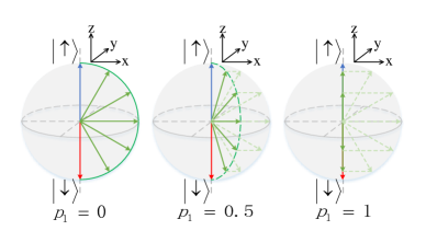
In Eq. (9), we know that skyrmion numbers are not affected by phase local decoherence unless revealing complete phase damping. In this case, the corresponding Stokes parameters are . As the damping factor is close to , the two components and approach while holds unchanged, producing the effect that the coherence between the two components of the optical skyrmion field gradually disappears and finally the output is a maximal mixed state. Therefore, topological stability is maintained as long as coherence is preserved, as shown in Fig. 1(a).
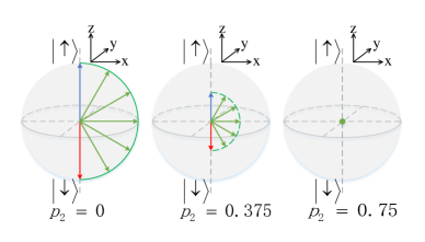
For depolarizing channel, due to the final Stokes parameters are in proportion to the initial values, i.e. , the Stokes parameters after being normalized in local decoherence are identical and invariant except for the case of . Therefore, we have the analytical solution in Eq. (10) and the skyrmion number remains constant related to (when ). The illustration is in Fig. 1(b).
(a)Phase damping channel
(b)Depolarizing channel
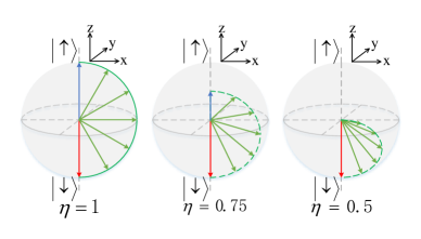
(c)Amplitude damping channel
Figure 1: Diagrams of the spin vector change on the Bloch sphere after passing through the decoherence channel. The normalized Stokes parameters (polar angle: ; azimuthal angle: ), denote the unit vector on the Bloch sphere. We take a slice ( i.e. azimuth ) on the Bloch sphere as an example to observe the changes of spin vectors. (a) Phase damping channel: With the damping factor of PDC increases, and gradually decreases, whereas remains unchanged. Once , all the spin vectors will fall on the central axis and it is a maximal mixed state without coherence. (b) Depolarizing channel: As the damping factor of DC decreases, the three components of the Stokes parameters will proportionately contract towards the center of the sphere, eventually converging to a single point. (c) Amplitude damping channel: When , spin vectors can cover the whole Bloch sphere. When (like ), decreases and the magnitude of the blue spin vector pointing to the North Pole is reduced to half of its initial value. When , the blue spin vector vanishes and there are only spin vectors for the southern hemisphere.
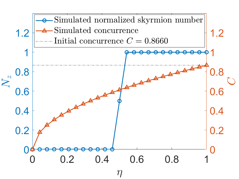
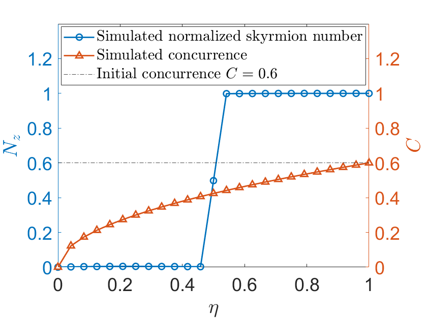
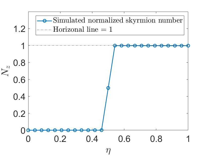
We can see that the occurrence of transition points of the first two channels are similar to the one in Ref. Ornelas et al. (2024) showing the absence of non-trivial topology of skyrmions once the entanglement vanishes. In the case of amplitude damping channel, we can find that it differs from the above and is the transition point of skyrmion numbers and skyrmion numbers hold invariant as long as the damping factor satisfies the condition . We explain this phenomenon as follows. The amplitude damping channel demonstrates a process of the decay of two-level (atom) system due to the spontaneous emission. {, } can be seen as the upper energy level (the excited state) and the lower energy level (the ground state) of this system, and initial populations are and , respectively. There is a probability of decaying from the excited state to the ground state so that final populations become and . As decreases, the population of the upper level gradually decreases. When , the inequality is always true. It is well-known that skyrmions is a mapping from to containing the whole solid angle, however, it will only map half of the Bloch sphere and topological spin textures will also be destroyed once , as shown in Fig. 1(c).
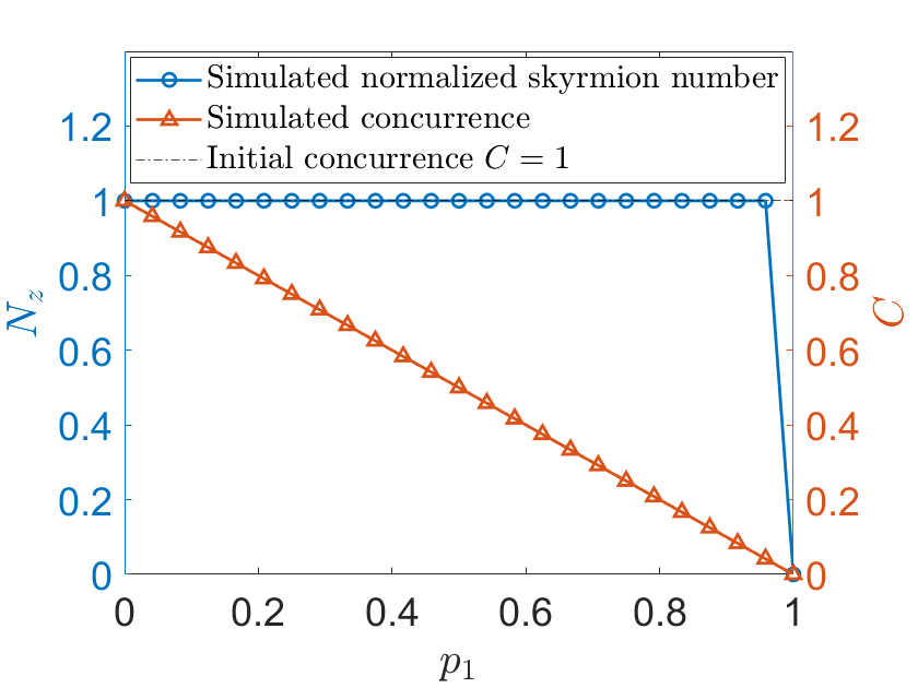
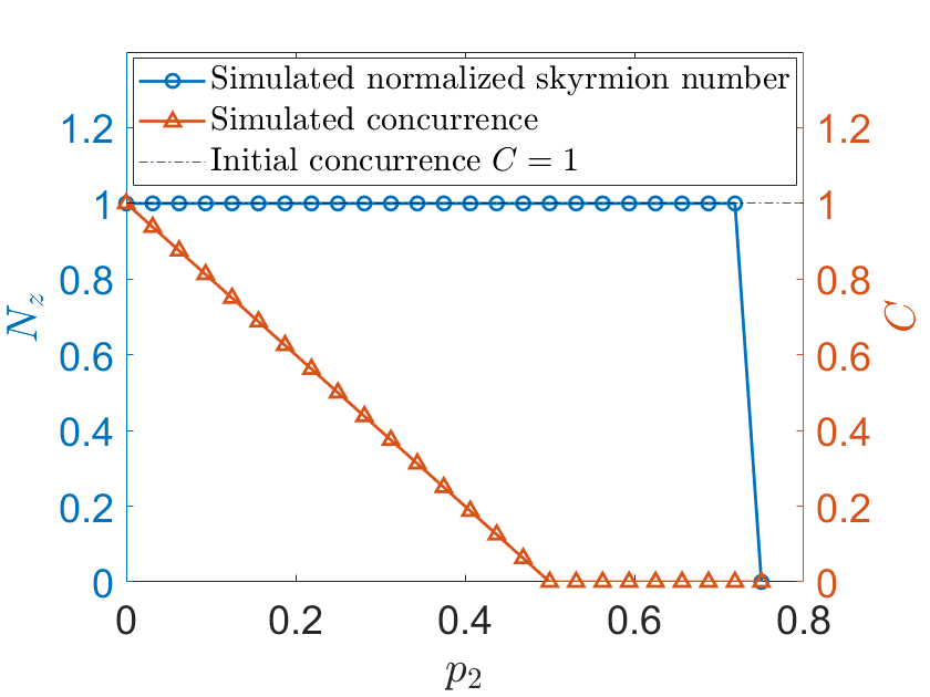
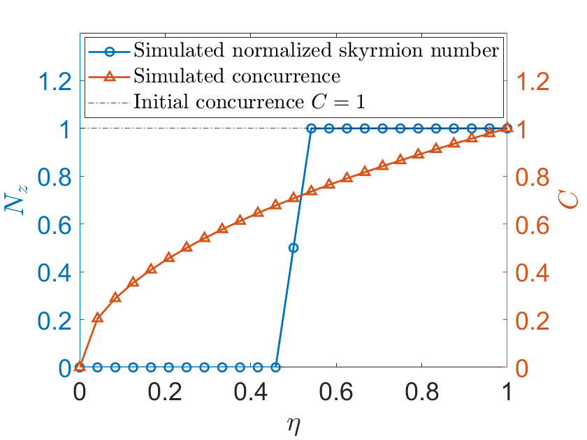
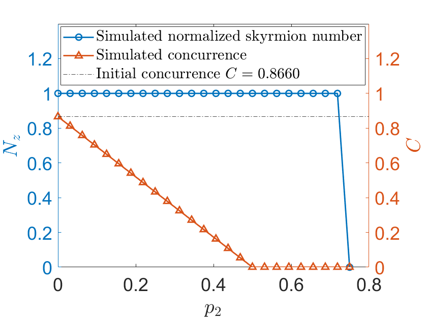
Meanwhile, we numerically demonstrate the results that the normalized skyrmion numbers vary with damping factors in three local decoherence channels in Fig. 2. Here, we consider that initial scale coefficients satisfy and the azimuthal indices of two OAM modes are and . It is obvious that these numerical results in Fig. 2(a), 2(b) and 2(c) (represented by curves with hollow circles in blue) are in good agreement with the analytic solutions in Eq. (9), (10) and (11). Additionally, Eq. (8) shows that the occurrence of these transition points is independent of the initial state. Apart from the case of maximum entanglement (i.e. ), as long as and , all trends hold.
(a)Phase damping channel
(b)Depolarizing channel
(c)Amplitude damping channel
Figure 2: Normalized skyrmion numbers and relevant concurrence. Blue curves with hollow circles represent simulated normalized skyrmion numbers, corresponding orange curves with plus signs represent simulated concurrence values, and black dotted lines are initial concurrence values (here it is with ). (a) Phase damping channel: the damping factor corresponds to . (b) Depolarizing channel: the damping factor corresponds to . (c) Amplitude damping channel: the damping factor is .
Compared the skyrmion number with the entanglement degree between two DOFs characterized by a quantity named concurrence Hill and Wootters (1997); Wootters (1998); Yu and Eberly (2004), there is evidence that the skyrmion number does not change entirely synchronously with entanglement during local decoherence. We obtain the analytical formulas about concurrence in three channels in the following
(12)
(13)
(14)
And the numerical curves of concurrence in Fig. 2 is perfectly fitted with theoretical values. In phase damping channel and amplitude damping channel, the concurrence approaches zero when complete coherence damping occurs, as shown in Fig. 2(a) and 2(c). For depolarizing channel in Fig. 2(b), however, it behaves very differently. The concurrence goes to prematurely, a phenomenon known as entanglement sudden death Yu and Eberly (2006); Almeida et al. (2007); Cui et al. (2008); Yu and Eberly (2009); Meng et al. (2020), which describes the complete loss of quantum correlation (or entanglement) in a finite time rather than an asymptotic decay over an infinite duration. More details are in Appendix. As shown in Fig. 2, due to the presence of transition points of skyrmion numbers, the skyrmion number is more robust than concurrence in these cases.
Intensity loss of two polarization components is also an aspect to consider and we can characterize the loss by two loss parameters and . In fact, the loss parameters have no influence on the stability of skyrmion numbers unless at least one component is lose completely. Because the variations of loss parameters and are equivalent to the variations of the scale coefficients and . More details can be found in Appendix.
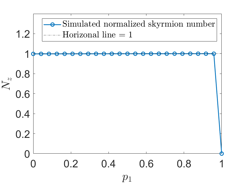
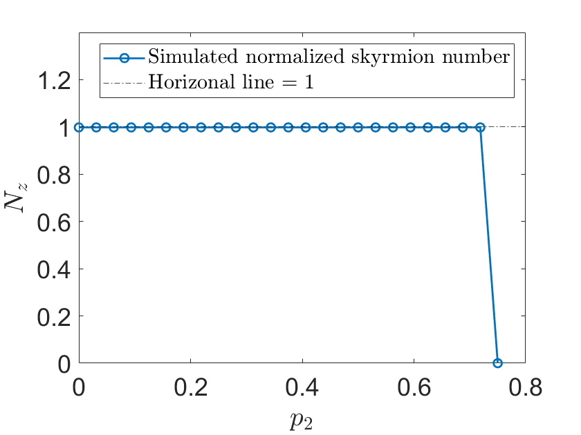
All of the above studies are based on a homogeneous decoherence process, where the damping factors are uniformly distributed in space (i.e. a constant). Extending this investigation, we find that the topological resilience of an optical skyrmion field propagating through an inhomogeneous yet continuous local decoherence channel still persists. We numerically generate an inhomogeneous local decoherence channel, where the damping factor varies randomly across the spatial domain and the correlation of damping factors between any two positions is characterized by a specific correlation length Goodman (2007). The continuity of damping factors of the channel is supposed to be guaranteed by increasing the correlation length because the skyrmion numbers are unaffected by the operations of smooth deformations Ornelas et al. (2024). The numerical grid size is . Consequently, when , the inhomogeneous channel deteriorates into a homogeneous one. The results are shown in Tab. 1 and we perform 50 realizations for the ensemble average on account of the existence of random process. Similarly to the uniform case, we confirm numerically that the skyrmion numbers remain stable and the topology is preserved in these instances: (1) in phase damping channel; (2) in depolarizing channel; (3) and (the continuity of the channel is better) in amplitude damping channel. More details are in Appendix.
PDC
DC
ADC
1
0.9986
1.0000
0.9186
2
0.9999
1.0000
0.9589
4
1.0000
1.0000
0.9849
8
1.0000
1.0000
0.9964
16
1.0000
1.0000
0.9993
32
1.0000
1.0000
1.0000
64
1.0000
1.0000
1.0000
128
0.9998
1.0000
1.0000
256
0.9995
1.0000
1.0000
512
0.9966
1.0000
1.0000
Table 1: Normalized skyrmion numbers in the inhomogeneous local decoherence channels with different types and different correlation lengths in units of a single grid point. is the simulated skyrmion number and is the theoretical skyrmion number. For phase damping channel, the damping factor ; For depolarizing channel, the damping factor ; For amplitude damping channel, the damping factor .
Discussion and conclusion.—We have investigated the topological resilience of skyrmions in three local decoherence scenarios. Both analytically and numerically, we have proven the validity of this topological property. By considering a 2D optical skyrmion field constructed by paraxial LG spatial modes with two orthogonal polarization states, we have found that the two skyrmion numbers and in phasing noise and depolarizing noise maintain invariant unless their damping factors and reach their respective maximum values indicating completely damping. Moreover, as the decoherence strength increasing, the skyrmion number remains topologically stable until the damping factor of amplitude noise is less than or equal to , which means that the topological spin texture is destroyed and the mapping from to is also incomplete. The immunity against local decoherence endowed by skyrmions’ topology is independent of the scale coefficients and spatial modes’ azimuthal indices of the initial state. Due to the existence of transition points of skyrmion numbers in local decoherence, the skyrmion numbers are more robust than the concurrence in these cases. And we also demonstrate numerically that these features are still valid for inhomogeneous yet continuous decoherence channels.
In this paper, we consider two DOFs of a particle to create the optical skyrmion field. The analysis is not restricted by this condition, and our results continue to be applicable to common systems (two-level single-particle or two-level single-particle ensemble system), inspiring additional generalization among skyrmions in optics and magnetism. Meanwhile, compared with the pure states and unitary channels in Ref. Nape et al. (2022); Ornelas et al. (2024), we employ more general expressions and non-unitary channels to study the stability of skyrmion numbers. The robustness of skyrmion numbers can be used to guide the transmission of classical discrete signals. It is expected that topological resilience in local decoherence has greater application prospects in more research fields, including communication, information encoding and processing, metrology and imaging.
Note added.—We notice that there is a similar work Koch et al. (2024) when our paper is in preparation. Our work differs from the work in Ref Koch et al. (2024): we consider single-particle systems rather than entangled bi-photon states. Our findings are applicable to classical optical fields and can be generalized to other physical systems, as long as the noise in those systems is localized.
Acknowledgments.—This work was supported by the National Natural Science Foundation of China (No. 92065113), Innovation Program for Quantum Science and technology (No. 2021ZD0301201) and the University Synergy Innovation Program of Anhui Province (No. GXXT-2022-039).
Nagase et al. (2019)T. Nagase, M. Komatsu,
Y. G. So, T. Ishida, H. Yoshida, Y. Kawaguchi, Y. Tanaka, K. Saitoh, N. Ikarashi, M. Kuwahara, and M. Nagao, Phys. Rev. Lett. 123, 137203 (2019).
Taguchi et al. (2001)Y. Taguchi, Y. Oohara,
H. Yoshizawa, N. Nagaosa, and Y. Tokura, Science 291, 2573
(2001).
Neubauer et al. (2009)A. Neubauer, C. Pfleiderer, B. Binz,
A. Rosch, R. Ritz, P. G. Niklowitz, and P. Böni, Phys. Rev. Lett. 102, 186602 (2009).
Ritz et al. (2013)R. Ritz, M. Halder,
M. Wagner, C. Franz, A. Bauer, and C. Pfleiderer, Nature 497, 231 (2013).
Mochizuki et al. (2014)M. Mochizuki, X. Yu,
S. Seki, N. Kanazawa, W. Koshibae, J. Zang, M. Mostovoy, Y. Tokura, and N. Nagaosa, Nature Materials 13, 241 (2014).
Malozemoff and Slonczewski (2013)A. P. Malozemoff and J. C. Slonczewski, Magnetic domain
walls in bubble materials: advances in materials and device research, Vol. 1 (Academic press, 2013).
Heinze et al. (2011)S. Heinze, K. Von Bergmann, M. Menzel, J. Brede,
A. Kubetzka, R. Wiesendanger, G. Bihlmayer, and S. Blügel, Nature Phys. 7, 713 (2011).
Romming et al. (2013)N. Romming, C. Hanneken,
M. Menzel, J. E. Bickel, B. Wolter, K. von Bergmann, A. Kubetzka, and R. Wiesendanger, Science 341, 636 (2013).
Nape et al. (2022)I. Nape, K. Singh,
A. Klug, W. Buono, C. Rosales-Guzman, A. McWilliam, S. Franke-Arnold, A. Kritzinger, P. Forbes, A. Dudley, and A. Forbes, Nature Photonics 16, 538 (2022).
Jani et al. (2021)H. Jani, J.-C. Lin,
J. Chen, J. Harrison, F. Maccherozzi, J. Schad, S. Prakash, C.-B. Eom, A. Ariando, T. Venkatesan,
and P. G. Radaelli, Nature 590, 74 (2021).
Zdagkas et al. (2022)A. Zdagkas, C. McDonnell,
J. Deng, Y. Shen, G. Li, T. Ellenbogen, N. Papasimakis, and N. I. Zheludev, Nature Photonics 16, 523 (2022).
Cuevas et al. (2017a)A. Cuevas, M. Proietti,
M. A. Ciampini, S. Duranti, P. Mataloni, M. F. Sacchi, and C. Macchiavello, Phys. Rev. Lett. 119, 100502 (2017a).
Cuevas et al. (2017b)A. Cuevas, A. Mari,
A. De Pasquale, A. Orieux, M. Massaro, F. Sciarrino, P. Mataloni, and V. Giovannetti, Phys.
Rev. A 96, 012314
(2017b).
Duncan and Kirkpatrick (2008)D. D. Duncan and S. J. Kirkpatrick, in Complex
dynamics and fluctuations in biomedical photonics V, Vol. 6855 (SPIE, 2008) pp. 23–30.
I Appendix
.1 Skyrmion numbers
Skyrmions are a type of topological spin textures characterized by corresponding topological numbers, i.e. skyrmion numbers. For the electron spin, the normalized local magnetization defines the relevant skyrmion field. In turn, for the light beam, a normalized Stokes vector is introduced to calculate the skyrmion number. An optical skyrmion can be regarded as a mapping from a transverse spatial plane to a Poincaré sphere (or a Bloch sphere in spin) , which has a two-dimensional (2D) surface of a three-deimensional (3D) ball and completely covers a solid angle, and the skyrmion number denotes the number of times of wrapping . The th component of the skyrmion field can be expressed by Gao et al. (2020)
(S1)
where the notations and are both Levi-civita symbols and the subscript . Nevertheless, we only need to exploit the th component
(S2)
where is spatially distributed, i.e. . Therefore, the skyrmion number is described as Gao et al. (2020)
(S3)
.2 Stokes parameters
To calculate skyrmion numbers, we need to obtain relevant Stokes parameters and this operation is also called Stokes measurements. The input state of this system is written in the general form , where and {} are two mutually orthogonal states. Here, we consider paraxial Laguerre-Gaussian (LG) modes with no radial index () and the is be described as
(S4)
where is a normalization constant, is the generalized Laguerre polynomial, is the Rayleigh distance, represents the beam wavelength, is the beam waist of the fundamental mode, and is the beam radius at the plane.
The initial density matrix is
(S5)
where , , , , , , and other coefficients are zero. The Stokes parameters correspond to the expected values of measurement operators of the overall system, i.e.
(S6)
where is the trace operator, the position basis of orbital angular momentum (OAM) degree of freedom (DOF) satisfies the orthogonality and the completeness relation . By employing Eq. (S5) into Eq. (S6), we can get
(S7)
where .
For the term , we can rewrite it by the eigenvalue decomposition method, i.e. . So Eq. (S7) can be expressed by
(S8)
where and are the projection operators. Therefore, we can calculate the three locally normalized Stokes components of the initial density matrix in detail.
(S9)
(S10)
(S11)
where , and is the total intensity in the skyrmionic beam. In fact, is the first or second term of Eq. (S8) after the eigenvalues are removed. These states are the eigenvectors of three Pauli operators , respectively.
(, , , , , .)
Each is
(S12)
(S13)
(S14)
(S15)
(S16)
(S17)
Substituting Eq. (S12)-(S17) into Eq. (S9)-(S11), we can obtain the final forms of locally normalized Stokes parameters
(S18)
(S19)
(S20)
And the three elements satisfy the vector normalization relation .
.3 Analytical solutions of skyrmion numbers in local decoherence
We primarily consider three decoherence channels, i.e., phase damping channel, depolarizing channel and amplitude damping channel. The decoherence channels are solely acting on the polarization DOF and OAM DOF maintains unaffected by imposing on an identity operator . We use Kraus operators to characterize these channels.
.3.1 A. Phase damping channel
For phase damping channel, the output state is
(S21)
and this channel can be related by the Kraus operators . Kraus operators have the property of . If we input a density matrix of a single qubit ,
the output density matrix after the channel is
(S22)
The final density matrix of the phase damping channel is (from the initial state in Eq. (S5))
(S23)
where , , , , and other coefficients are zero. The locally normalized Stokes parameters are
(S24)
(S25)
(S26)
The equality must be fulfilled and we simplify the two LG spatial modes ( and ) into the following form
(S27)
where .
In the polar coordinate , we can get
(S28)
(S29)
(S30)
(S31)
(S32)
(S33)
where . The relevant th component of the field and the skyrmion number respectively are
(S34)
(S35)
.3.2 B. Depolarizing channel
For depolarizing channel, the output state is
(S36)
and the Kraus operators of this channel are
(S37)
If we input a density matrix of a single qubit ,
the output density matrix after the channel is
(S38)
The final density matrix of the depolarizing channel is
(S39)
where , , , , , , and other coefficients are zero. The Stokes parameters in depolarizing channel differ only by a factor from the Stokes parameters in the input state, and this factor has no effect after vector normalization. Thereby the locally normalized Stokes parameters in depolarizing channel are the same as Eq. (S18), (S19) and (S20):
(S40)
(S41)
(S42)
Here, and
where .
Then
(S43)
(S44)
(S45)
(S46)
(S47)
(S48)
The relevant th component of the field and the skyrmion number respectively are
(S49)
(S50)
.3.3 C. Amplitude damping channel
For amplitude damping channel, the Kraus operators are
(S51)
is the damping factor. If we input a density matrix of a single qubit ,
the output density matrix after the channel is
(S52)
The initial state in Eq. (S5) goes through an amplitude damping channel, the final state can be presented by
(S53)
where , , , , , and other coefficients are zero. The locally normalized Stokes parameters are
(S54)
(S55)
(S56)
Similarly, the equality must be fulfilled.
Furthermore, we simplify the two LG spatial modes ( and ) into
where . From it, we know that the specific values of scale coefficients and have no impact on the calculation of skyrmion numbers (). After that, Eq. (S54)-(S56) can be simplified to
(S57)
(S58)
(S59)
Then
(S60)
(S61)
(S62)
(S63)
(S64)
(S65)
where . By using the Eq. (S2), we get the th component of the field
.4 Different initial scale coefficients and corresponding skyrmion numbers
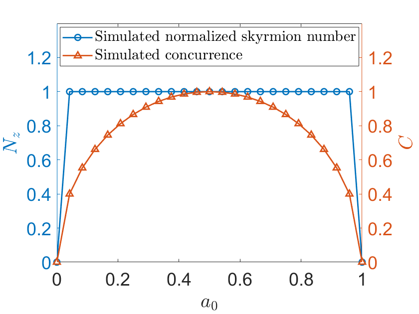
An initial state of the system is and the scale coefficients can vary prompting different initial concurrence values under the condition of normalization (i.e. ). However, different values of and do not influence the trend of skyrmion numbers, regardless of the presence or absence of local decoherence.
Firstly, we examine the case without decoherence in Fig. S1. Here, and . By varying , we obtain different initial states. However, the skyrmion numbers remain topologically stable and unchanged unless the degree of entanglement vanishes. This result is consistent with the one in Ref. Ornelas et al. (2024).
Figure S1: The simulated normalized skyrmion numbers and concurrence values vary with scale coefficient in the case of no decoherence.
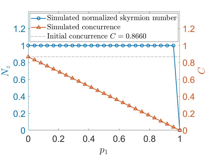
Secondly, in the main text, we study the case of maximum entanglement degree (concurrence ) with the presence of local decoherence channels. In Fig. S2 and S3, the scale coefficients are and , respectively. But different initial states have the same results so that each critical transition point of skyrmion numbers in local decoherence is impervious.
(a)Phase damping channel
(b)Depolarizing channel
(c)Amplitude damping channel
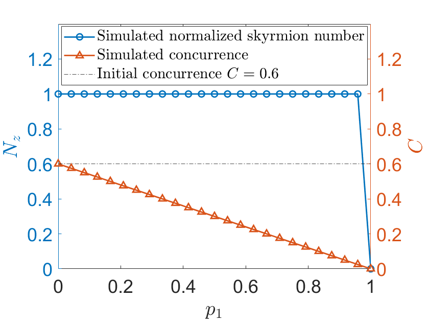
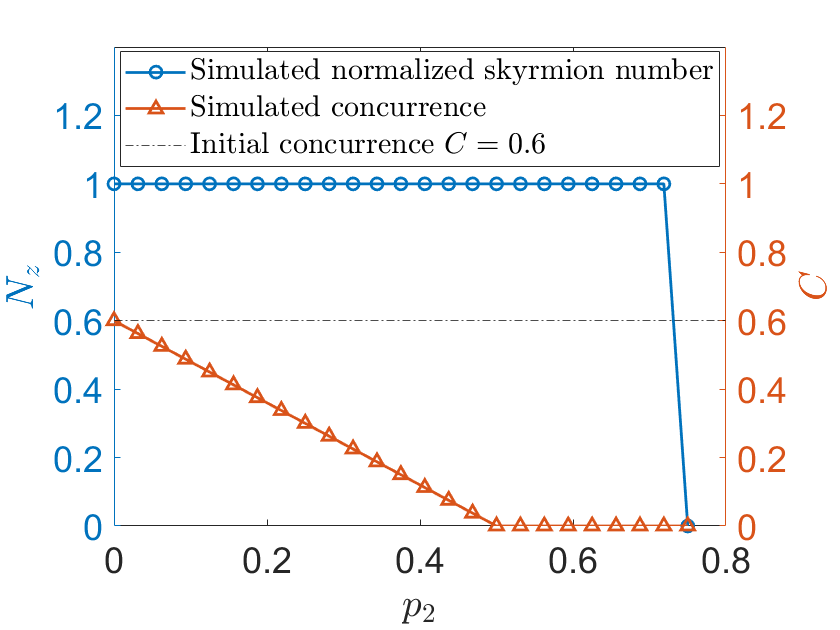
Figure S2: The simulated normalized skyrmion numbers and concurrence values in different local decoherence channels. The scale coefficients , and correspond to an initial concurrence of .
(a)Phase damping channel
(b)Depolarizing channel
(c)Amplitude damping channel
Figure S3: The simulated normalized skyrmion numbers and concurrence values in different local decoherence channels. The scale coefficients , and correspond to an initial concurrence of .
In addition, in the main text, we take two LG modes with azimuthal indices as an example to interpret skyrmions’ properties. In Fig. S4, we make a smaller value with , and the features of skyrmions are all the same.
(a)Phase damping channel
(b)Depolarizing channel
(c)Amplitude damping channel
Figure S4: The simulated normalized skyrmion numbers in different local decoherence channels. The azimuthal indices of two spatial modes are and . The scale coefficients , and correspond to an initial concurrence of .
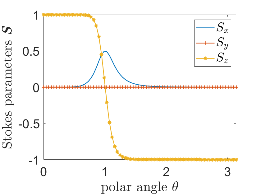
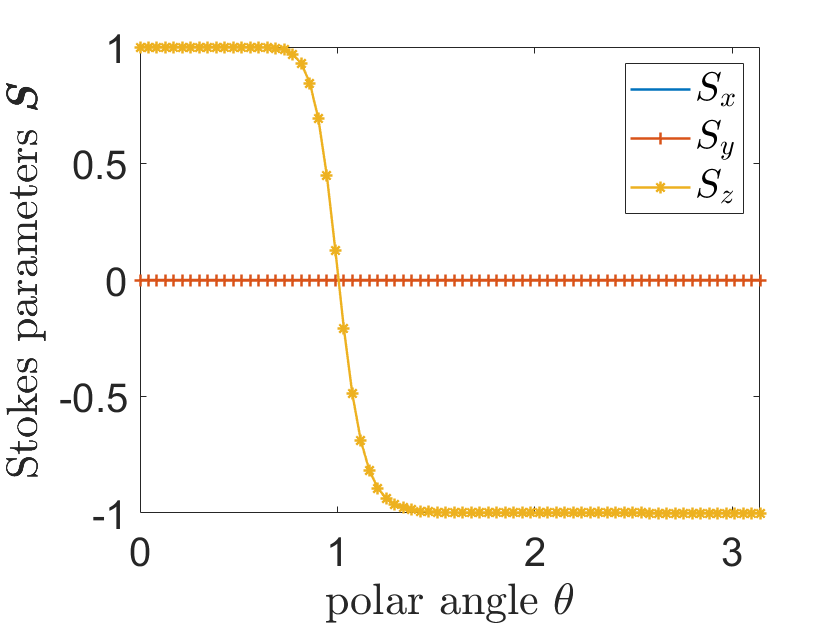
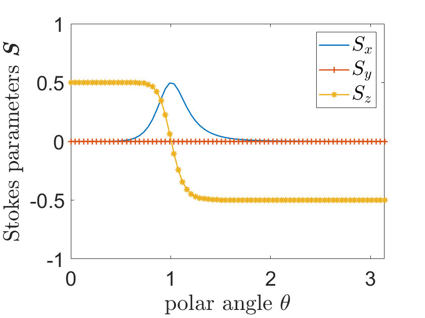
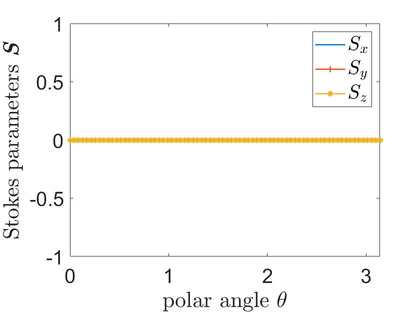
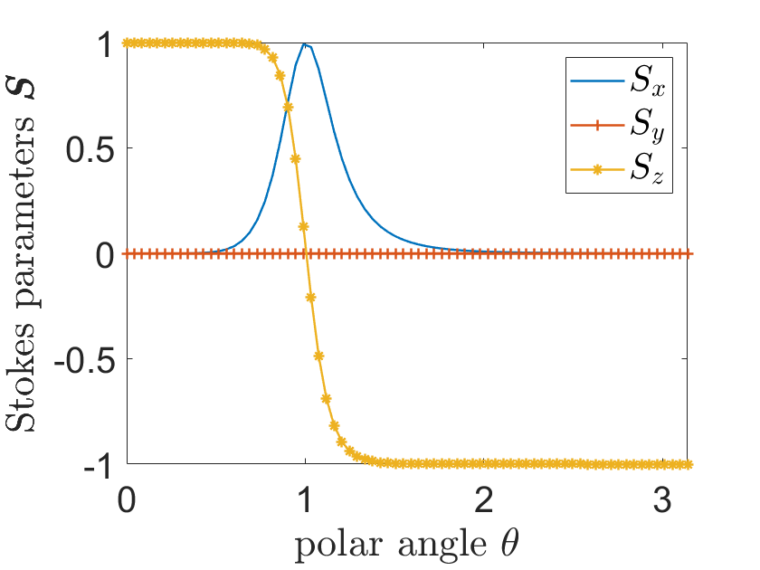
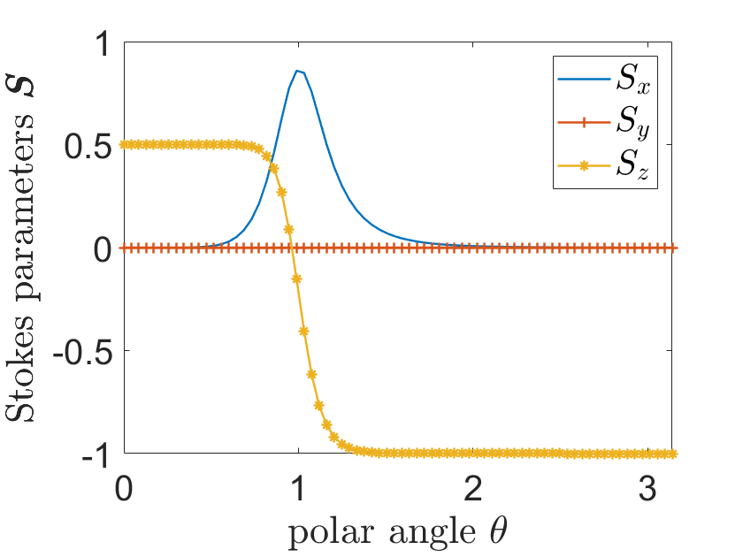
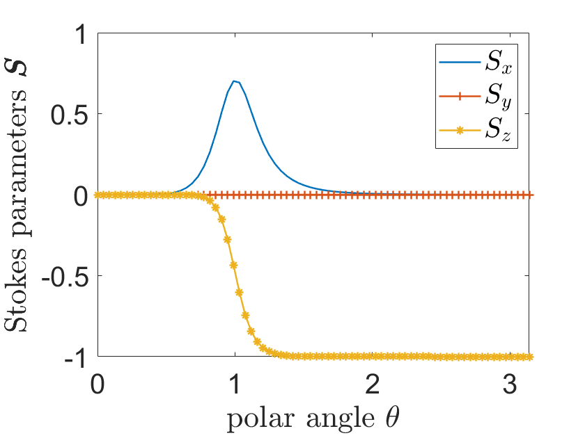
.5 The Stokes parameters vary with the decoherence strength
An ordinary state is usually denoted by a density matrix which can be expanded using the identity and three Pauli matrices . For a 2D density matrix, it can be expressed by , and the vector , (where ), is called the Bloch vector pointing in the spin direction. Actually, the 3D Stokes parameters equivalently represent the spin vector direction in the Bloch sphere. We numerically demonstrate the variations of the Stokes parameters with different decoherence strength. Taking a slice of azimuthal angle (i.e. ) as an example, we observe the curves in Fig. S5, S6, S7. In Fig. S5, the component of the Stokes parameters, , remains invariant yet the component of the Stokes parameters is fading and eventually , resulting in complete decoherence. In Fig. S6, as the decoherence strength increases, both and decrease until they reach zero. In Fig. S7, gradually decreases with increasing decoherence strength of amplitude damping channel, while becomes unable to reach the upper hemisphere when the damping factor .
(a)
(b)
(c)
Figure S5: The Stokes parameters vary with different decoherence strength () of phase damping channel. We choose a slice of as an example.
(a)
(b)
(c)
Figure S6: The Stokes parameters vary with different decoherence strength () of depolarizing channel. We choose a slice of as an example.
(a)
(b)
(c)
Figure S7: The Stokes parameters vary with different decoherence strength () of amplitude damping channel. We choose a slice of as an example.
.6 Entanglement sudden death (ESD)
The interaction between two entangled qubits and the surrounding noisy environment may provoke the dissipation or/and dephasing effects and even the loss of quantum correlation. Quantum correlation can be quantified by the concurrence which varies between of classical correlation and of maximal entanglement. The expression of concurrence is and are the positive eigenvalues in decreasing order of the operator Almeida et al. (2007). We generally use the term ‘decoherence’ to describe the decay and loss of quantum correlation or entanglement and there is some research that shows only local decoherence is sufficient to lead to ESD Yashodamma et al. (2014); Almeida et al. (2007); Bavontaweepanya (2018). ESD is a phenomenon that entanglement of a system vanishes in a finite time and it is different from the asymptotic decay in a infinite time. For three decoherence channels, there are distinct features.
In phase damping channel, the concurrence conforms to . When , the density matrix corresponds to the maximally mixed state and the entanglement completely vanishes.
In depolarizing channel, the final density matrix is in the Eq. (S38) and the upper bound of is . The depolarizing channel with can map any input to the maximally mixed state. The concurrence is . When , the concurrence is zero, which reveals the occurrence of ESD.
In amplitude damping channel, from the Eq. (S52), the atom always stays at the ground state if . The concurrence in amplitude damping channel is , showing no ESD as entanglement does not completely vanish until .
Obviously, depolarizing noise can cause finite-time entanglement decay yet phasing noise and amplitude noise have no ESD.
.7 The skyrmion numbers in loss
When we consider the loss of two polarization components of the optical skyrmion field, there are two types of possible cases, i.e., the equal loss parameters and unequal loss parameters. The unnormalized state is expressed as
(S68)
where and are the loss parameters of two components, respectively. and indicate no loss and (or ) means the skyrmion number of the field is zero. Similarly, we can calculate the corresponding skyrmion numbers by Eq. (S3).
If , the normalized state is
(S69)
The output density matrix is
(S70)
where is the normalized coefficient. Comparing Eq. (S70) with Eq. (S5), they differ only by a factor that has no impact on computing the locally normalized Stokes parameters in Eq. (S18-S20). Thus, the skyrmion number remains constant when the two polarization components have equal loss parameters unless .
If and , the normalized state is
(S71)
the output density matrix is
(S72)
where is the normalized coefficient.
We can rewrite the normalized state in Eq. (S71) using new coefficients and , i.e.,
(S73)
where , and . Eq. (S73) is equivalent to the state .
, , , , , , and other coefficients are zero.
Thus the skyrmion number in this case exhibits the same stability as in the case of the pure state without decoherence in Sec. .4, i.e., the skyrmion number remains stable unless the degree of entanglement vanishes ( or ) described by Ref. Ornelas et al. (2024).
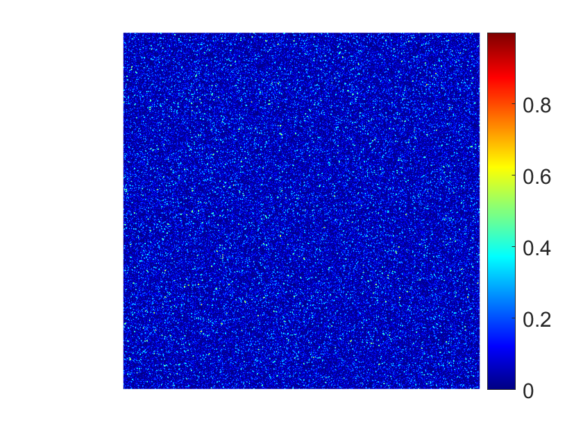
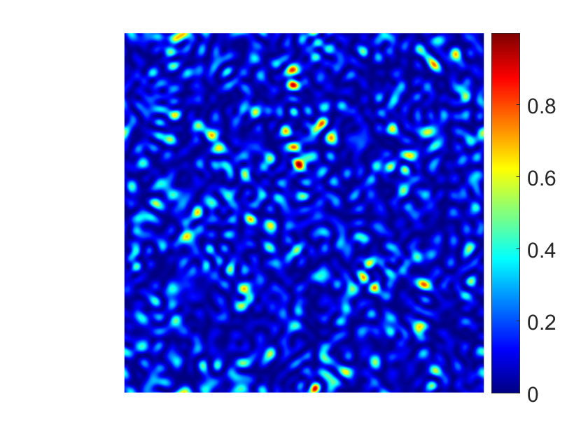
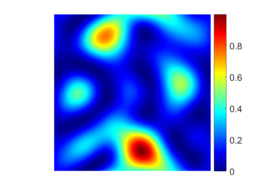
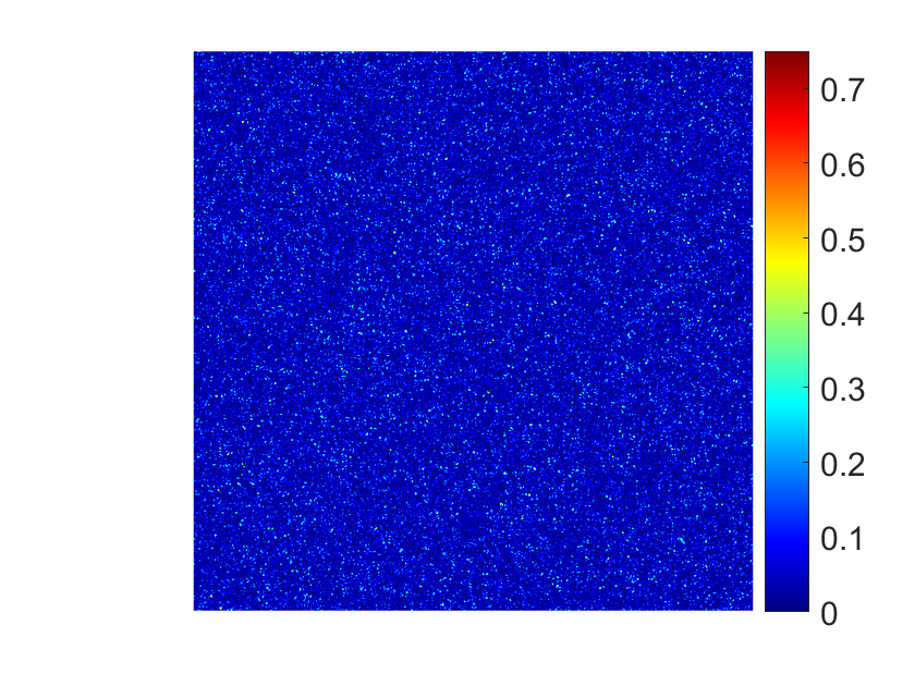
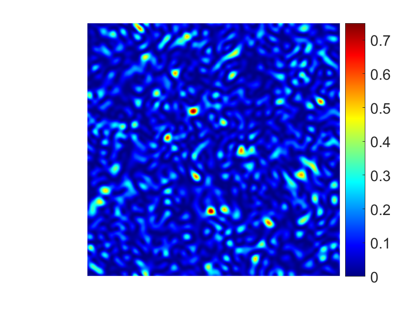
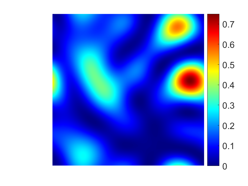
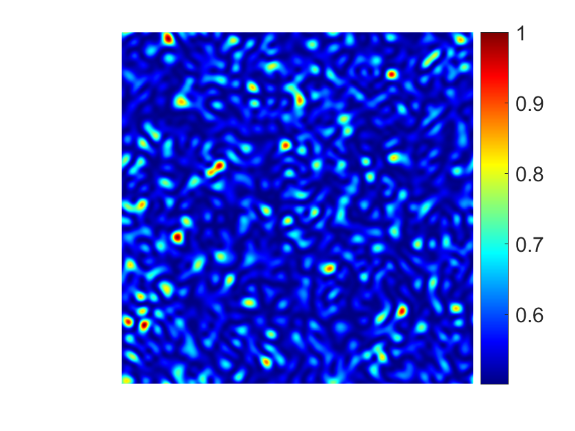
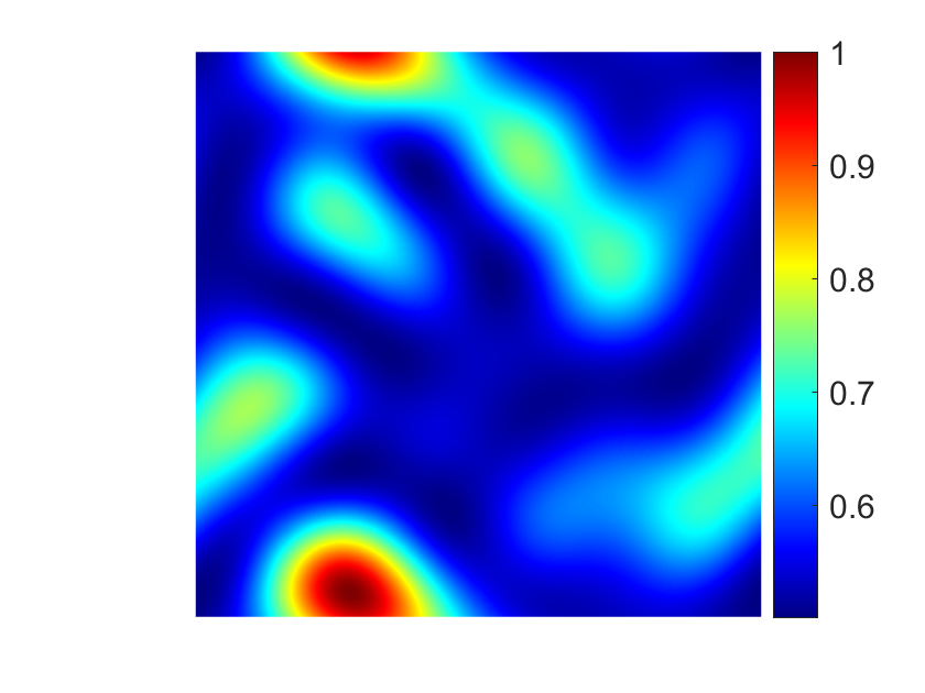
.8 Generation of inhomogeneous yet continuous decoherence channels
To generate a decoherence channel with a spatially distributed yet continuous damping factor, we control the correlation length of distribution and use the Fourier transform method Goodman (2007); Duncan and Kirkpatrick (2008). Considering a screen size of (with ), we first create a Gaussian complex random matrix of size (with ), filling the elements of . Then, we apply the Fourier transform to the entire matrix and finally obtain the modulus squared of the matrix as the desired result. For example, in Fig. S8, S9, S10, we demonstrate several inhomogeneous distributions of the damping factors in three local decoherence scenarios with different correlation lengths.
(a) grids
(b) grids
(c) grids
Figure S8: Phase damping channel. The numerical screen size of grid is , and we create three spatial distributions of the damping factor with different correlation lengths ( grids) as examples.
(a) grids
(b) grids
(c) grids
Figure S9: Depolarizing channel. The numerical screen size of grid is , and we create three spatial distributions of the damping factor with different correlation lengths ( grids) as examples.
(a) grids
(b) grids
(c) grids
Figure S10: Amplitude damping channel. The numerical screen size of grid is , and we create three spatial distributions of the damping factor with different correlation lengths ( grids) as examples.