AdaSemiCD: An Adaptive Semi-Supervised Change Detection Method Based on Pseudo-Label Evaluation

Abstract

Change Detection (CD) is an essential field in remote sensing, with a primary focus on identifying areas of change in bi-temporal image pairs captured at varying intervals of the same region by a satellite. The data annotation process for the CD task is both time-consuming and labor-intensive. To make better use of the scarce labeled data and abundant unlabeled data, we present an adaptive dynamic semi-supervised learning method, AdaSemiCD, to improve the use of pseudo-labels and optimize the training process. Initially, due to the extreme class imbalance inherent in CD, the model is more inclined to focus on the background class, and it is easy to confuse the boundary of the target object. Considering these two points, we develop a measurable evaluation metric for pseudo-labels that enhances the representation of information entropy by class rebalancing and amplification of confusing areas to give a larger weight to prospects change objects. Subsequently, to enhance the reliability of sample-wise pseudo-labels, we introduce the AdaFusion module, which is capable of dynamically identifying the most uncertain region and substituting it with more trustworthy content. Lastly, to ensure better training stability, we introduce the AdaEMA module, which updates the teacher model using only batches of trusted samples. Experimental results from LEVIR-CD, WHU-CD, and CDD datasets validate the efficacy and universality of our proposed adaptive training framework.

I Introduction

Change detection (CD) has emerged as a significant research focus within the field of remote sensing in recent years. Its objective is to identify regions of interest that have experienced alterations in bi-temporal image pairs captured at varying times of the same geographical area using satellite technology. This method plays a crucial role in remote sensing data analysis and is of particular importance in various civilian sectors such as urban planning [1, 2], rural land management [3, 4], and disaster assessment [5, 6].

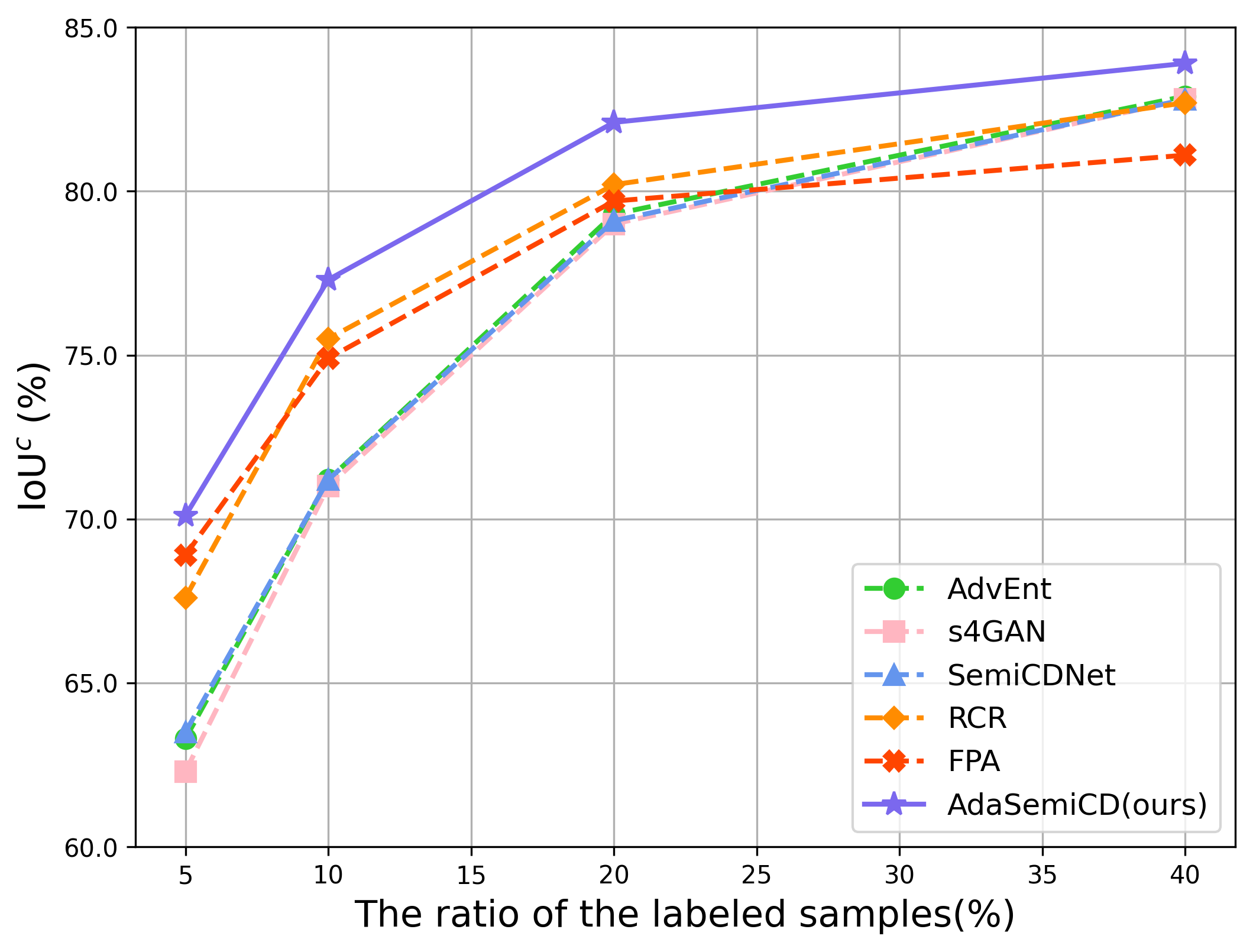
Figure 1: Comparison between SOTA semi-supervised methods and our AdaSemiCD on the CDD Dataset.

Given that the process of accurately annotating masks for change detection tasks is notably labor intensive, direct application of traditional supervised learning approaches, such as CNN [7, 3, 8, 9, 4] and Transformers [10, 11, 12], to a limited set of labeled data often results in limited performance. In response to these challenges, researchers have investigated a range of approaches such as Self-supervised learning(SSL)[13, 14],Unsupervised Change Detection (USCD) [15, 16, 17], Weakly Supervised Change Detection (WSCD) [18, 19, 20], and sample generation strategies [21, 22, 23, 24]. Although WSCD is cost-efficient, it is reliant on incomplete or inaccurate labels, which can introduce substantial errors and unpredictably noisy data. USCD, on the other hand, does not require labeled data and utilizes the intrinsic patterns present in the data, but it often faces challenges when tackling specific tasks like classification or detection. Sample generation strategies, which include data augmentation [23], generative adversarial networks (GANs) [22], and diffusion models [24], frequently necessitate the simulation or synthesis of additional data. However, when dealing with limited available samples, these methods may encounter constraints due to insufficient diversity in the generated data, which can diminish the model’s ability to generalize. As a result, semi-supervised change detection (SSCD) [25, 26, 27] emerges as a potentially more effective solution. The paradigm of semi-supervised learning [28, 29, 30] is to enhance CD performance by leveraging the limited available labels and the large volume of unlabeled samples. Usually, researchers generate pseudo-labels for the unlabeled data to act as guidance during training. These pseudo-labels are often temporary predictions with higher probabilities. The most prevalent approach is the Mean-Teacher [31] framework, which employ a teacher model to generate pseudo-labels that serve as guidance for the student model during the training process. The teacher model is subsequently updated using the exponential moving average (EMA) [32] of the student model. By training on a mix of limited data with actual labels and abundant data with pseudo-labels, the student model can learn more significant features, leading to noticeable enhancements in performance.

While these methods produce acceptable outcomes, significant problems persist: the model indiscriminately treats all samples, irrespective of their quality, and the training process lacks flexibility. Firstly, it’s evident that unlabeled samples may not always function as efficient ‘teachers’. Models frequently encounter difficulties in generating reliable high-quality pseudo-labels for intricate samples, which in turn introduces extra noise that can misguide the model’s training.

Subsequently, the EMA updating process does not take into account the quality of samples. Given that training batches can be biased or contain noise, dynamically determining the training update timing could contribute to the stability of the training process. These factors underscore the need for a more precise supervisory approach, failing which it could negatively impact the model’s training. In this study, we introduce an adaptive dynamic learning strategy, AdaSemiCD, designed to improve the accuracy of pseudo-labels and streamline the training process. Our framework incorporates the traditional semi-supervised training approach, augmented by two innovative functional modules, AdaFusion and AdaEMA. Initially, we utilize AdaFusion to suppress noise at the individual sample level, thereby enhancing the accuracy of pseudo-labels. Contrary to previous methods like Augseg [33] or CutMix [34] that relied on entirely random fusion regions, our AdaFusion technique proactively identifies the most uncertain region and substitutes it with reliable content from either labeled datasets or unlabeled datasets of superior quality. Following this, we dynamically adjust the rate of parameter updates in the teacher-student model via AdaEMA to ensure improved stability. Although the traditional EMA effectively mitigates fluctuations in model parameters, thereby boosting stability, it persists in uniformly updating after each training iteration, overlooking the model’s varying learning outcomes across different iterations when handling a range of training samples. If unlabeled samples contain an abundance of erroneous information, it can misdirect the model’s training. Therefore, our AdaEMA introduces an adaptive selection process for model-level parameter updates, enabling the model to fully integrate superior parameters.

In summary, the main contributions of this paper are as follows.

• We propose an adaptive SSCD framework named AdaSemiCD, which dynamically improves the pseudo-labels as well as adjusts the training procedure with pseudo label quality assessment.

• We propose an AdaFusion strategy to enhance unreliable unlabeled samples. The fusion region and the trusted contents are selectively chosen with the uncertainty map.

• We propose an AdaEMA parameter update strategy, which updates the teacher model with a batch-wise pseudo-labels improving assessment.

• Experimental results on publicly available datasets LEVIR-CD, WHU-CD, and CDD demonstrate the effectiveness of our method.

II Related Work

II-A Semi-supervised learning

The technique of semi-supervised learning (SSL) applies supervised learning to a small subset of labeled data and unsupervised learning to a larger pool of unlabeled data. SSL is mainly categorized into three strategies: consistent regularization (CR), self-training, and holistic methods. The last strategy combines the first two strategies within an SSL framework.

CR techniques are grounded in the concept of perturbed consistency, which utilizes the coherence between the model’s output after varying degrees of perturbed input data as a training constraint. The three consistent regularization frameworks, in ascending order, including: the ${\Pi}$-model [35], the Temporal-ensembling model [35], and the Mean-teacher (MT) model [32]. The ${\Pi}$-model’s double-branch network shares the weight; the Temporal-ensembling model amalgamates all the outputs in the time series, with each image’s pseudo-labels being the EMA of the previously generated results; the MT model carries out this smoothing operation at the model parameters level. This model has found application in subsequent semi-supervised research across various domains, such as Active-Teacher for semi-supervised object detection [36], [37, 38, 33, 39] for semi-supervised general semantic segmentation,  [40] for image classification, and  [41][42] for semi-supervised medical image segmentation. There has also been explored in the area of perturbation design, with [43] and [25] examining the image-level perturbation and feature-level perturbation of CR respectively.

In the realm of self-training methods, the authenticity of pseudo-labels is of paramount importance. This has led to extensive research into the effective selection of high-quality pseudo-labels for supervised learning. [44] employs a set probability threshold as a selection standard. ST++ [45] has developed a multi-tier self-training structure, where labels of high confidence are used for self-training repeatedly until all unlabeled samples have been utilized. [46] uses a constant entropy value as the filtering limit.

More often than not, CR and self-training are not used independently, but rather in conjunction, forming a comprehensive approach to semi-supervised learning. This is exemplified in [38, 33, 39, 40] and [45], as partially discussed in earlier sections.

II-B Semi-supervised Change Detection

Since annotating a large number of images for CD is time-consuming, recent methods mainly focus on the SSCD. In the realm of CR techniques, the incorporation of the mean teacher model in CD was first introduced by Bousias et al. [47]. However, the initial outcomes did not show considerable potential, as this SSCD method fell short when compared to a benchmark that exclusively used a restricted quantity of labeled data for entirely supervised learning. Despite increasing labeled data, this disparity continues to expand. Using this as a basis, Mao et al.[48] implemented minor and major improvements to the inputs of the teacher and student models, respectively. Furthermore, they formulated an extra teacher-virtual adversararial training component to further reduce the harmful effects of the pseudo label noise.

Additionally, other semi-supervised methods employ either a single model or a two-branch model with shared weights. Such as Sun et al. [49] introduce a siamese network. They incorporated additional self-training based on pseudo-labels, employing threshold filtering to eliminate low-quality pseudo-labels. The rationale behind this filtering lies in the potential noise introduced by pseudo-labels with low confidence, which could adversely affect SSL training. Hafner et al. [50] propose a dual-task SSCD framework that combines building segmentation and change detection, two closely related downstream tasks. They devised a novel consistency constraint between the two change detection masks produced by the Siamese segmentation network and the change detection network. Bandara et al. [25] explored feature-based perturbations of the regularization term, applying various data perturbations at the feature level to expand the distribution space of consistency constraints. This approach fully leverages the information embedded in unlabeled samples, and in recent work, Zhang et al. [27] imposed two constraints of class consistency and feature consistency on unlabeled datasets. By aligning the feature representations of unlabeled samples on varying and invariant classes, the model could learn from a feature space that is closer to the real distribution, this contributed to the renewal of the best performance record at that time.

Other methods predominantly utilize Generative Adversarial Network (GAN), which were initially proposed by Ian J. Goodfellow in 2014[51]. Some methods use GAN to learn the feature distribution space close to the real labeled data[26, 52, 53, 54]; The other part uses GAN to generate data samples[55, 56]; The more noteworthy research in the recent work is [18] proposed a new paradigm for change detection, unifying unsupervised, weakly supervised, regionally supervised, and fully supervised change detection into an end-to-end framework. While these endevavors have reported great success in SSCD, the highly unstable training of GAN makes hyperparameter adjustment become s challenging. Additionally, the issue of gradient disapperance frequently arises during the training phase. Morever, the strong discriminatory capaality of the discriminator can lead to imbalanced performance between the generator and discriminator of the GAN if no additional training techniques are implementrd. Consquently, achieving the idealized optimal scenario is challenging, making the pritical application of this method somewhat intricate. So we continue the semi-supervised framework of consistent and self-teinging.

III METHODOLOGY

Fig. 2 provides a comprehensive summary of our AdaSemiCD framework, aiming to enhance the SSCD performance by utilizing the scarce labels and vast quantity of unlabeled samples. We commence with a broad introduction of the framework, followed by an in-depth explanation of the uncertainty map used to assess our pseudo-labels, and finally present the specifics of AdaFusion and AdaEMA.

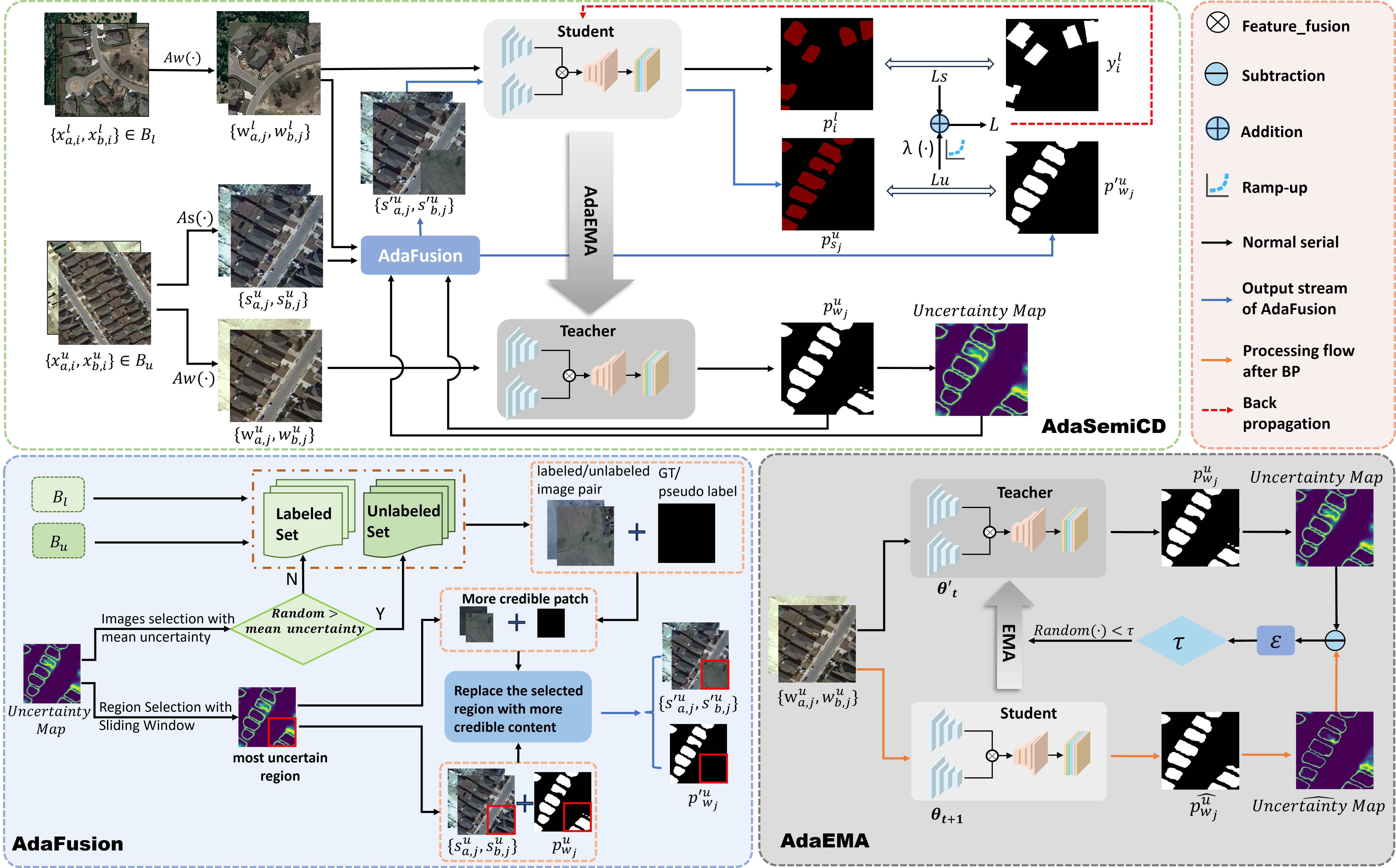
Figure 2: The overview of the proposed AdaSemiCD framework, and details of two novel modules. Our approach is based on the common teacher-student training pipeline for SSCD, and we suggest utilizing the AdaFusion module to produce samples with increased reliability and the AdaEMA module to enhance the efficiency of EMA update times.

III-A Overview of the AdaSemiCD Framework

The task of semi-supervised change detection can be described as follows: Given a labeled dataset $\displaystyle{D}_{l}=\left\{\left\{\smash{x_{a,i}^{l},x_{b,i}^{l}}\right\},y_{i}^{l}\right\}_{i=1}^{m}$ and an unlabeled dataset $\displaystyle{D}_{u}=\left\{x_{a,j}^{u},x_{b,j}^{u}\right\}_{j=1}^{n}$, where $\left\{\left\{\smash{x_{a,i}^{l},x_{b,i}^{l}}\right\},y_{i}^{l}\right\}$ represents the i-th pair of labeled image pairs and their ground truth, and $\left\{\smash{x_{a,i}^{u},x_{b,i}^{u}}\right\}$ represents the i-th pair of unlabeled image pairs, subscripts a and b are used to identify the images before and after phases respectively, and the number of samples with and without labeled datasets is n and m, $n\gg m$, the model $M$ is expected to not only extract meaningful information from ${D}_{l}$ but also capture a wider range of features by utilizing numerous unlabeled training samples in ${D}_{u}$ to improve the model’s generalization capabilities.

Model architecture: In this study, we employ the widely-used teacher-student framework for SSCD tasks. The network is composed of two components, a student model $M_{stu}$ and a teacher model $M_{tea}$ that shares the same structure. The student model is trained to extract significant features from a small number of labeled samples and a large volume of unlabeled samples, with the aid of optimization via gradient descent methods. Conversely, the teacher model $M_{tea}$ generates pseudo-labels to guide the student in assimilating unlabeled data, and the teacher model is refreshed using EMA methods.

Usually, samples undergo either weak $A_{w}(\cdot)$ or strong $A_{s}(\cdot)$ augmentation processes prior to being input into the network to maintain high-quality generalization performance.

Objectives: The objective is to minimize the supervised loss $\mathcal{L}_{s}$ on $D_{l}$ while also ensuring consistency on disturbed $D_{u}$ with a minimal $\mathcal{L}_{u}$. During training, samples are fed into the network in randomly shuffled batches, $\mathcal{B}_{l}$ and $\mathcal{B}_{u}$.

The loss $\mathcal{L}_{s}$ for labeled samples within a batch $B_{l}$ is calculated as the cross entropy (CE) of ground truth $y_{i}^{l}$ and it’s prediction $p_{i}^{l}$:

$$\mathcal{L}_{s}=\frac{1}{\left|\mathcal{B}_{l}\right|}\sum_{i=1}^{\left|\mathcal{B}_{l}\right|}\mathrm{CE}\left({p}_{i}^{l},y_{i}^{l}\right),$$ (1)

where $|\mathcal{B}_{l}|$ represents the mini-batch’s size, ${p}_{i}^{l}$ represents the CD result of the $i$-th pair images.

The loss $\mathcal{L}_{u}$ for unlabeled samples within a batch $B_{u}$ is quite similar. Here we use the pseudo-labels from $M_{tea}$ as supervision for the prediction from $M_{stu}$. And $\mathcal{L}_{u}$ is calculated as:

$$\mathcal{L}_{u}=\frac{1}{\left|\mathcal{B}_{u}\right|}\sum_{j=1}^{\left|\mathcal{B}_{u}\right|}\mathrm{CE}\left(p_{s,j}^{u},{p}_{w,j}^{u}\right),$$ (2)

where $|\mathcal{B}_{u}|$ represents the size of unlabeled image mini-batch, ${p}_{w,j}^{u}=M_{tea}^{\theta^{\prime}}(w_{a,j}^{u},w_{b,j}^{u})$ represents the detection result of the teacher model on the change of the i-th pair of unlabeled images weakly augmented, and ${p}_{s,j}^{u}={M_{stu}^{\theta}(s_{a,j}^{u},s_{b,j}^{u})}$ represents the detection result of the teacher model on the change of the i-th pair of unlabeled images by further strongly augmented.

To sum up, the total loss for the training procedure of AdaSemiCD is:

$$\mathcal{L}=\mathcal{L}_{s}+\lambda(\cdot)\mathcal{L}_{u}$$ (3)

Previous studies[40, 41] have employed a constant value for $\lambda(\cdot)$. However, we argue that this approach is not suitable for single-stage semi-supervised learning algorithms. During the initial training phases, the pseudo-labels generated by our model for unlabeled samples are highly unreliable; excessive reliance on unsupervised training at this stage can introduce significant noise. Conversely, as training progresses into the middle and later stages, the model increasingly learns from the limited labeled data, leading to an improvement in the quality of the pseudo-labels. This justifies a reduction in the proportion of supervised training relative to unsupervised training. To mitigate overfitting and enhance the feature space, it is essential to implement a controlled process to dynamically adjust the contribution of these two components in the loss function. As the pseudo-labels in the starting stage are quite unstable, we use a ramp-up process to control the training pace of the unlabeled part. $\lambda(\cdot)$ denotes the time varing weight of unsupervised loss, which is a function changing with training step and used to dynamically adjust the proportion of supervised and unsupervised training in different stages.

$$\lambda(\cdot)=w_{max}\times e^{-\phi\times\left(1-iter_{cur}/iter_{max}\right)^{2}}$$ (4)

where $w_{max}$ and $\phi$ are hyperparameters, $w_{max}$ representing the maximum weight of unsupervised loss, $\phi$ is used to control the severity of the ramp-up; $iter_{cur}$ represents the current iteration cycles; $iter_{max}$ is the total number of ramp-up cycles, is obtained by multiplying $\gamma$ and the total number of training iterations, and $0\textless\gamma\textless 1.0$; After the ramp-up process, the weight of unsupervised losses remains $w_{max}$ and does not change. In the early stage of training, this weight is relatively low, and unsupervised training plays a negligible role, but in the middle and later stages of training, this weight gradually increases and the unsupervised loss after weighting exceeds the supervised loss, so unsupervised training accounts for the main part.

Training strategy: The student network’s parameters $\theta$ are adjusted by Stochastic Gradient Descent(SGD) technique to reduce the overall loss $\mathcal{L}$, while the teacher network’s parameters $\theta^{\prime}$ are updated by the exponential moving average of the student model’s parameters $\theta$ over the time series, as depicted in Eq. 5. The hyperparameter $\beta$ acts as a momentum parameter. The larger the value of $\beta$, the broader the moving metric average window becomes. Typically, $\beta$ is chosen to be a number near 1.0, for instance, 0.996 in this study.

$$\theta^{\prime}=\beta\theta^{\prime}+(1-\beta)\theta$$ (5)

Proposed modules: The essence of semi-supervised learning lies in the quality of pseudo-labels. Nevertheless, it’s apparent that the previously mentioned procedure does not take into account the diverse effects of individual samples on training. This paper concentrates on two elements that are directly related to the generation of pseudo-labels: the initial pair of unlabeled images, and the efficiency of the pseudo-label-generation network, also known as the teacher model, in identifying changes. To offer more dependable supervisory data to unlabeled information and reduce training uncertainty, we’ve designed an adaptive training strategy to tackle these two key issues. Our initial proposal is to develop a metric that can measure the uncertainty of pseudo-labels, serving as the basis for adaptive modifications. Following that, we suggest making adaptive changes at the image level to the unlabeled training samples and suitably integrating reliable contents. Furthermore, it includes applying adaptive and selective EMA updates to the teacher network during the training phase to limit variations, thus producing more consistent and superior quality pseudo-labels. These efforts are elaborated in the subsequent sections.

III-B Pseudo-label qualification metric

To enhance the effectiveness of pseudo-labels by accurately gauging their quality, a crucial step is the implementation of an evaluation metric. This metric will be instrumental in identifying reliable labels and determining the utility of each training sample. Unlike the scenario with labeled image pairs where real labels serve as a benchmark for assessing the model’s inference quality through average intersection over union, F1 scores, and so forth, pseudo-labels lack any such reference points and can only be compared to themselves. Therefore, we have devised a quantifiable evaluation metric specifically for pseudo-labels, designed to increase the total information entropy while taking into account factors like category imbalance and areas of confusion.

To evaluate the quality of pseudo-labels, a frequently employed technique for this is the computation of information entropy [57],

$$E(x_{i})=-P\left(x_{i}\right)\log_{2}P\left(x_{i}\right),$$ (6)

where $P\left(x_{i}\right)$ is the output probability of a trained model on sample $x_{i}$. Our conviction is that a lower information entropy in the predicted value corresponds to a greater trustworthiness of the prediction outcome. On the contrary, a higher information entropy leads to a more varied prediction outcome, a more evenly distributed prediction probability on the same pixel, and a diminished distinction in the category.

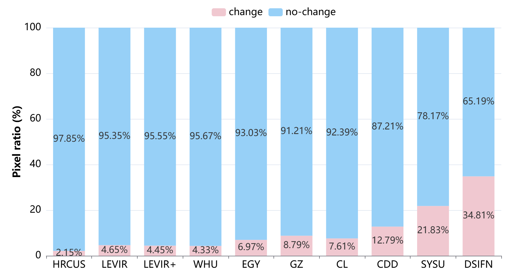
Figure 3: Class statistics of common CD datasets. The proportion of the changed/unchanged categories is extremely unbalanced.

In our change detection task, the direct application of entropy often does not yield good results due to the significant challenge posed by category imbalance. As illustrated in Fig. 3, ten publicly available change detection datasets were evaluated, namely HRCUS-CD[58], LEVIR-CD[59], LEVIR-CD+[59],WHU-CD[60], EGY-CD[61], GZ-CD[26], CL-CD[62], CDD[63], SYSU-CD[64] and DSIFN-CD[65]. The ratios of the changed and unchanged categories are highly skewed. This significant category imbalance can lead to our model inadequately learning the target categories during training while disproportionately capturing feature distributions from background categories. As a result, there is an increased tendency to classify pixels as belonging to the background class during inference. Consequently, although the overall accuracy (OA) of the model appears high, the performance on the Intersection over Union (IoU) across various categories remains unsatisfactory. To minimize the influence of this category imbalance when assessing the quality of pseudo-labels, we assigned different weights to the two categories when computing information entropy as Eq. 7.

$$E^{\prime}\left(X\right)=w_{1}\times E\left(x_{i}\right)[0]+w_{0}\times E\left(x_{i}\right)[1],$$ (7)

where $w_{0}$ and $w_{1}$ represent the proportions of pixels in the current batch that belong to the unchanged and changed categories, respectively. The formulas for their calculation are given by Eq. 8 and Eq. 9.

$$w_{0}=\frac{\sum_{i=1}^{|Bu|}\sum_{k=1}^{H\times W}{(P(x_{i})==0)}}{{|Bu|}\times H\times W}$$ (8)

$$w_{1}=\frac{\sum_{i=1}^{|Bu|}\sum_{k=1}^{H\times W}{(P(x_{i})==1)}}{{|Bu|}\times H\times W}$$ (9)

Moreover, pixels from diverse areas contribute in varying manners. Pixels of greater importance, like those in boundary, target, and regions similar to the background, who are offenly predicted with large uncertainty, should receive more emphasis. Initially, we enhance the impact of these essential regions by computing the absolute value of the disparity between the prediction probabilities of the two categories.

$$D\left(x_{i}\right)=abs(P\left(x_{i}\right)[1]-P\left(x_{i}\right)[0])$$ (10)

Here, $abs$ signifies absolute value, a measure taken to prevent the inconsistencies that may arise from varying changes both prior to and following a phase. Then doing pixel-level product operation with information entropy, we get the uncertainty map of image $(x_{i})$,

$$U\left(x_{i}\right)=1-D\left(x_{i}\right)\cdot E^{\prime}\left(x_{i}\right)$$ (11)

Clearly, in pixel locations with low information entropy, this process won’t result in notable alterations, whereas in pixel locations with high information entropy, the absolute value of the predictive probability post-subtraction will be significantly reduced, and the immediate amalgamation will diminish its importance. Consequently, we adopt the inverse of rectified information entropy as its depiction.

To sum up, with the goal of evaluating the quality of pseudo-labels for change detection, we put forward a measurable calculation metric $U$ to gauge uncertainty, which enhances the overall information entropy considering factors like category imbalance and focus on areas of confusion.

III-C AdaFusion: Adaptive sample fusion

Image fusion is frequently employed to augment samples and boost generalization, with CutMix[34] and MixUp[66] being typical examples. In this study, our aim is to leverage image fusion techniques to exclude the unreliable areas in a training sample. This procedure involves two steps: region selection, which decides the location of the operation, and image selection, which decides the content to be used.

Adaptive selection of fusion region. Contrary to the conventional CutMix technique, which arbitrarily chooses blending regions, our approach is more refined. Initially, we would select a bounding box with random size, then slide the window, and choose the area where the total of uncertainty is highest as the region to be combined, using Eq. 11.

These regions are frequently boundaries or intricate areas where it’s challenging to identify targets. The CutMix fusion can guarantee the variety of samples and simultaneously decrease the unsupervised noise.

Adaptive selection of fusion contents. For the region of maximum uncertainty, we have the option to choose a substitute from its corresponding samples from the label section $B_{l}$ or the unlabeled section with higher probabilities $B_{u}$. This strategy prevents overuse of only labeled samples and further mitigates the risk of overfitting. The focus of the content here is confined to the contrast between labeled and unlabeled image pairs, rather than a more detailed distinction (such as the level of the image or the level of the object). This is because we suggest that too much human intervention could potentially undermine the model’s capacity to generalize. The choice of fusion content is mainly accomplished by adaptively adjusting a threshold that determines whether to fuse with a labeled image pair. We directly use the computed uncertainty as the threshold, and if the randomly generated probability exceeds the total uncertainty of the sample, the labeled images in the training batch are randomly selected as the fusion content. If not, other unlabeled image pairs in the batch are randomly selected. It is easy to understand that the higher the sample’s reliability, the better the quality of the pseudo-label. We consider it reliable enough to avoid the necessity for fusion with the limited labeled images, which could potentially increase the likelihood of overfitting. Samples with higher uncertainty come with more noise, and the addition of new content can significantly reduce the noise density.

III-D AdaEMA: Adaptive EMA update strategy

Within the teacher-student framework, the teacher model is obtained by integrating the moving exponential average of the student model across the time series. This approach is more stable and reliable compared to dual models with shared weights. However, our expectation for Mean-Teacher is to reach the optimal state of coevolution, where the teacher model is a cumulative representation of the evolving student model. The crucial element in achieving this co-evolution is whether the student model progresses or regresses each time the teacher model gets updated. So, how can we assess the state of the student model? This question is inherently related to the validation phase of the training process. Typically, after training for several epochs, we evaluate the current model, feed samples from the validation set into the model for inference, and compare the outcomes with the actual labels to determine accuracy. However, if we perform such validation after every iteration, it becomes highly computationally intensive, leading to a significant increase in training time. Lowering the number of samples in the validation set (to just a few pairs) might address the feasibility issue, but it also presents new challenges when the sample size is too small to thoroughly assess the model’s performance. So, is there a middle ground that can merge these two concepts?

Algorithm 1 The AdaEMA algorithm.

0:    Student model $M_{stu}^{\theta}$, Teacher model $M_{tea}^{\theta^{\prime}}$ The set of training samples for current batch $\mathcal{B}=\left\{\mathcal{B}_{l},\mathcal{B}_{u}\right\}$;

0:    Updated Teacher model, $M_{tea}^{\hat{\theta}}$;

1:  Calculate the loss $\mathcal{L}_{s}$ on labeled samples $\mathcal{B}_{l}$ with Eq. 1; 

2:  Calculate the loss $\mathcal{L}_{u}$ on unlabeled samples $\mathcal{B}_{u}$ with Eq. 2; 

3:  Update the student model $M_{stu}^{\theta}$ to $M_{stu}^{\theta^{\prime}}$ by SGD to minimize the total loss following Eq. 3; 

4:  Calculate the uncertainty ${U}_{tea}$ of pseudo-labels generated on $\mathcal{B}_{u}$ by the teacher model $M_{tea}^{\theta^{\prime}}$according to Eq.11; 

5:  Calculate the uncertainty ${U}_{stu}$ on $\mathcal{B}_{u}$ by updated student model $M_{stu}^{\theta^{\prime}}$ according to Eq.11; 

6:  Calculate the upper bound on the probability of update $\tau$ according to Eq. 12 and Eq. 13;

7:  if $random(\cdot)<\tau$ then

8:     Update the teacher model to $M_{tea}^{\hat{\theta}}$ by Eq. 5; 

9:  else

10:     $M_{tea}^{\hat{\theta}}=M_{tea}^{\theta^{\prime}}$; 

11:  end if

12:  return  $M_{tea}^{\hat{\theta}}$.

At each training phase, we initially update the student model’s parameters, denoted as $M_{stu}^{\theta}$, following the training strategy described in section III-A, resulting in $M_{stu}^{\theta^{\prime}}$. Next, we evaluate both the updated student model $M_{stu}^{\theta^{\prime}}$ and the teacher model $M_{tea}^{\theta^{\prime}}$ on the current batch of unlabeled training samples $\mathcal{B}_{u}$. We determine the ensuing uncertainty map using Eq. 11, and denote these as $U_{tea}$ and $U_{stu}$. The progression is marked by changes in uncertainty, as illustrated in Eq. 12.

$$\varepsilon=\frac{\sum{U_{stu}}-\sum{U_{tea}}}{|B_{u}|}.$$ (12)

If $\varepsilon$ is below zero, the model either degrades or oscillates. In contrast, when $\varepsilon$ is zero or higher, the model progresses. Ultimately, only the student models that have evolved successfully are selected to refresh the teacher model, with the maximum probability of update $\tau$ being derived as presented in Eq. 13.

$$\tau=\left\{\begin{array}[]{cl}\frac{1}{iter^{2}+\epsilon}&,\quad\varepsilon\leq 0\\ 1.0&,\quad\varepsilon>0\\ \end{array}\right.,$$ (13)

Here, $\epsilon=1e-5$ is used to prevent the divisor from being zero, and $iter$ denotes the present iteration count. If the model parameters are not selected for updating the Teacher model, they are not discarded outright. Instead, they are given a lower probability of being updated. With this upper bound regulation (ranging from 0 to 1), some randomness is introduced to determine the likelihood of updating the teacher network’s parameters. Further details are available in Algorithm 1.

IV Experiement

This section pertains to the experimental validation we performed. Initially, we present the assessment standards for experimental outcomes and the experimental datasets. Subsequently, we executed ablation experiments to validate the significance of each component in the methodology. Ultimately, we draw comparisons with the cutting-edge semi-supervised change detection techniques, using measurable experimental metrics and perceptible visual outcomes.

IV-A Experimental setup

IV-A1 Datasets

Our method is empirically tested on ten benchmark datasets, namely the LEVIR-CD [59], LEVIR-CD+ [59], WHU-CD[60], EGY-CD[61], HRCUS-CD[58], Change Detection Dataset(CDD)[63], GZ-CD[26], DSIFN-CD[65], SYSU-CD[64] and CL-CD[62]. Among them, these datasets cover different resolutions (0.03m-2.0m), different data sizes (2400-20000 pairs), different annotation categories (binary or multiclass), and different time spans between image pairs (1-16 years), as summarized in the Table I.

TABLE I: Ten publicly available change detection datasets used in the experiment.

Category	Datesets	Spatial Resolution	Size	Annotated Samples	Time Spans	Download
	LEVIR-CD [59]	0.5m	1024 $\times$ 1024	637	5 to 14 years	Link
	LEVIR-CD+ [59]	0.5m	1024 $\times$ 1024	985	5 to 14 years	Link
	WHU-CD [60]	0.2m	15354$\times$32507	1	2012 to 2016	Link
	GZ-CD [26]	0.55m	Varying	19	2006 to 2019	Link
	EGY-BCD [61]	0.25m	256 $\times$ 256	6091	2015 to 2022	Link
Building	HRCUS-CD [58]	0.5m	256 $\times$ 256	11388	Varing	Link
	CDD[63]	0.03m-1.0m	256$\times$256	16000	Varing	Link
	DSIFN-CD [65]	Unknown	512$\times$512	3940	Unknown	Link
	SYSU-CD[64]	0.5m	256$\times$256	20000	2007 to 2014	Link
Multiclass	CL-CD [62]	0.5-2.0m	512$\times$512	600	2017 to 2019	Link

We followed the same setup for all datasets, we chose 5$\%$, 10$\%$, 20$\%$ and 40$\%$ as the proportion of labeled samples, where we followed the semi-supervised partitioning in [26, 25, 27] on LEVIR-CD and WHU-CD, and performed our own random partitioning on the other data sets, but we performed the experiment fairly in the same setup for all comparison methods.

IV-A2 Evaluation Metrics

To facilitate a straightforward comparison with the latest cutting-edge techniques, we employed intersection over union (IoU) scores and overall accuracy (OA) on evaluation datasets. Given the severe imbalance in CD categories and our primary concentration on the changed area, we use the IoU of the change category $IoU^{c}$, the calculation formula are as follows:

$$\mathrm{IoU}=\frac{\mathrm{TP}}{\mathrm{TP}+\mathrm{FP}+\mathrm{FN}}$$ (14)

$$\mathrm{OA}=\frac{\mathrm{TP}+\mathrm{TN}}{\mathrm{TP}+\mathrm{FP}+\mathrm{TN}+\mathrm{FN}}$$ (15)

Where $\mathrm{TP}$ represents the positive sample correctly predicted (the correct changing pixel), $\mathrm{TN}$ refers to the negative sample correctly predicted (the correct unchanged pixel), and $\mathrm{FP}$ denotes the positive sample wrongly predicted (the unchanged pixel wrongly detected), $\mathrm{FN}$ represents the negative sample wrongly predicted (the pixel missed as the unchanged pixel). For both metrics, the larger the value, the better the change detection performance of the model. In the change detection task, OA is high overall due to binary classification and unbalanced category envy.

IV-A3 Implementation Details

The common components of this experiment were tested under the same conditions as the methods we intend to compare them with. To prevent network structure from causing interference, we utilized ResNet50+PPM as our change detection network follow [25] and [27]. We set the initial learning rate at 0.01, which linearly decreases to 1e-4 with a momentum of 0.9, and trained all methods using the SGD optimizer. All models underwent 80 epochs of training, with each batch having a mini-batch size of 8 for both labeled and unlabeled training sets. Furthermore, all the enhancements employed were identical to those used in FPA[27], which include random flip, random resize ranging from 0.5 to 2.0, and random crop among the weak augmentations, along with the nine strong augmentations cited in [67]. Given the limited amount of labeled data, the model is highly sensitive to the pseudo-labels’ filtering threshold, leading us to set 0.95 as the threshold for all models in the experiments conducted on the ten datasets and we follow the experience in [25] to set $\phi$ to 5. All our experiments were carried out using PyTorch on four NVIDIA GeForce RTX 3090 GPUs.

IV-B Compare with the SOTA methods

In order to prove the superiority of our proposed method, we compare it with several of the most advanced semi-supervised change detection methods. [26], [25] and [27] refresh the last semi-supervised CD performance in chronological order. In addition, we also compare with two semi-supervised semantic segmentation modding methods[37] and [68].

IV-B1 Quantitative results

We conducted a complete experiment on ten datasets, Table II and Table III report our experimental results on the Building CD datasets and mutilclass CD datasets respectively. Sup.Only is the result of supervised training only on a limited subset of labeled dataset, while Oracle is the result of fully supervised training on the entire training dataset. It is worth noting that our method achieves the state-of-the-art performance in almost all partition settings across the all datasets. To be sure, all the semi-supervised CD methods performed better than the supervised methods in the corresponding partition setting in most cases, which proves the effectiveness of the semi-supervised methods in learning from a large number of unlabeled training samples, at the same time, the lead achieved by our method proves that our adaptive design for how to learn from unlabeled samples to more correct guidance is of practical significance.

Building CD Datasets: As shown in Table II, Our AdaSemiCD achieved the state-of-the-art(SOTA) performance on four of the datasets, and the average $IoU_{c}$ of LEVIR-CD, LEVIR-CD+, WHU-CD and HRCUS-CD increased by 3.1, 1.3, 1.7 and 0.4 percentage, respectively. The performance on GZ-CD and EGY-CD were slightly inferior to FPA[27] in some experimental settings, but still achieved optimal results at the extremely scarce labeled data of 5$\%$, and the second best results in some other experiments settings. It should not be ignored that our method meets or even exceeds the Oracle results using only 10$\%$ or 20$\%$ labeled data on LEVIR-CD, LEIVIR-CD+ and EGY-CD, because these Building-CD datasets are extremely class-unbalanced, and our method takes this into account. Its variation area is relatively regular, and the type of variation is relatively simple. The same trend can be observed in the results of the FPA, where the percentage of labeled data between 10$\%$ and 40$\%$ does not increase significantly in results.

In addition, from the experimental results, the overall accuracy(OA) of all methods on these binary change detection datasets is very high, because the background class accounts for the majority. OA is often directly corresponding to $IoU_{c}$, and a slight improvement in OA is reflected in a relatively significant improvement in $IoU_{c}$. Our AdaSemiCD improves OA in almost all datasets because it greatly eliminates noise and the guidance of false signals.

TABLE II: The average quantitative metrics of different CD methods on building change detection datasets. The highlighted parts in blue are the best results, and the underlined ones are the second best results.

Dataset	Method	5%			10%			20%			40%
		$IoU^{c}$	OA		$IoU^{c}$	OA		$IoU^{c}$	OA		$IoU^{c}$	OA
LEVIR-CD	Sup. only	61.0	97.60		66.8	98.13		72.3	98.44		74.9	98.60
	AdvEnt[68]	66.1	98.08		72.3	98.45		74.6	98.58		75.0	98.60
	s4GAN[37]	64.0	97.89		67.0	98.11		73.4	98.51		75.4	98.62
	SemiCDNet[26]	67.6	98.17		71.5	98.42		74.3	98.58		75.5	98.63
	RCR[25]	72.5	98.47		75.5	98.63		76.2	98.68		77.2	98.72
	FPA[27]	73.7	98.57		76.6	98.72		77.4	98.75		77.0	98.74
	AdaSemiCD	77.7	98.78		79.4	98.87		80.3	98.92		80.6	98.93
	Oracle	$IoU^{c}$=77.9 and OA=98.77
LEVIR-CD+	Sup. only	52.0	97.72		58.4	98.06		66.1	98.31		66.2	98.42
	AdvEnt[68]	52.2	97.68		59.9	98.11		65.9	98.37		68.0	98.51
	s4GAN[37]	46.5	97.25		51.4	97.66		62.8	98.18		67.2	98.46
	SemiCDNet[26]	52.6	97.66		60.7	98.24		64.8	98.37		66.1	98.38
	RCR[25]	64.9	98.25		67.5	98.45		68.5	98.52		68.4	98.51
	FPA[27]	64.6	98.30		67.3	98.40		70.3	98.64		69.0	98.59
	AdaSemiCD	66.7	98.49		68.8	98.51		70.6	98.63		70.9	98.64
	Oracle	$IoU^{c}$=70.5 and OA=98.63
WHU-CD	Sup. only	50.0	97.48		55.7	97.53		65.4	98.20		76.1	98.94
	AdvEnt[68]	55.1	97.90		61.6	98.11		73.8	98.80		76.6	98.94
	s4GAN[37]	18.3	96.69		62.6	98.15		70.8	98.60		76.4	98.96
	SemiCDNet[26]	51.7	97.71		62.0	98.16		66.7	98.28		75.9	98.93
	RCR[25]	65.8	98.37		68.1	98.47		74.8	98.84		77.2	98.96
	FPA[27]	66.3	98.45		57.4	97.69		62.5	98.48		73.1	98.69
	AdaSemiCD	67.8	98.62		70.8	98.70		74.7	98.86		79.6	99.13
	Oracle	$IoU^{c}$=85.5 and OA=99.38
GZ-CD	Sup. only	47.5	93.56		51.4	94.26		58.0	95.65		66.3	96.62
	AdvEnt[68]	48.6	94.39		50.9	94.89		60.2	95.79		66.2	96.58
	s4GAN[37]	50.8	94.38		52.4	94.98		60.8	95.94		64.2	96.39
	SemiCDNet[26]	48.4	93.58		49.7	94.79		59.0	95.66		66.3	96.57
	RCR[25]	50.8	93.82		50.8	94.69		62.5	96.07		67.8	96.61
	FPA[27]	51.2	93.92		58.9	95.78		63.1	96.26		68.2	96.82
	AdaSemiCD	51.6	94.56		57.1	95.57		62.4	96.21		68.0	96.75
	Oracle	$IoU^{c}$=69.0 and OA=96.93
EGY-CD	Sup. only	49.8	95.73		54.6	96.38		61.4	96.83		65.1	97.25
	AdvEnt[68]	52.7	96.01		57.8	96.58		62.6	96.86		64.0	97.19
	s4GAN[37]	52.9	95.94		58.6	96.50		64.7	97.09		64.9	97.27
	SemiCDNet[26]	52.4	96.00		57.9	96.31		62.8	96.95		63.8	97.19
	RCR[25]	58.1	96.50		61.9	96.77		63.9	97.08		64.2	97.18
	FPA[27]	57.5	96.52		60.1	96.86		65.2	97.25		65.7	97.34
	AdaSemiCD	59.0	96.55		60.5	96.80		65.0	97.20		67.4	97.39
	Oracle	$IoU^{c}$=67.6 and OA=97.54
HRCUS-CD	Sup. only	29.5	98.11		36.0	98.45		43.4	98.68		48.9	98.84
	AdvEnt[68]	29.1	98.11		36.9	98.40		42.5	98.61		48.8	98.71
	s4GAN[37]	25.0	97.86		28.2	98.24		40.1	98.62		50.3	98.85
	SemiCDNet[26]	28.4	98.00		34.7	98.44		44.1	98.68		48.5	98.74
	RCR[25]	36.1	98.36		42.1	98.69		45.3	98.76		49.6	98.66
	FPA[27]	35.2	98.37		43.7	98.65		46.7	98.82		51.2	98.81
	AdaSemiCD	37.8	98.59		42.6	98.70		48.1	98.84		50.8	98.87
	Oracle	$IoU^{c}$=59.0 and OA=99.06

TABLE III: The average quantitative metrics of different CD methods on multiclass change detection datasets. The highlighted parts in blue are the best results, and the underlined ones are the second best results.

Dataset	Method	5%			10%			20%			40%
		$IoU^{c}$	OA		$IoU^{c}$	OA		$IoU^{c}$	OA		$IoU^{c}$	OA
CDD-CD	Sup. only	60.4	94.25		67.9	95.46		75.6	96.59		82.3	97.56
	AdvEnt[68]	63.3	94.65		71.2	96.01		79.3	97.14		82.9	97.66
	s4GAN[37]	62.3	94.69		71.0	95.94		79.0	97.10		82.8	97.63
	SemiCDNet[26]	63.5	94.68		71.2	95.99		79.1	97.13		82.8	97.63
	RCR[25]	67.6	95.40		75.5	96.57		80.2	97.26		82.7	97.61
	FPA[27]	68.9	95.66		74.9	96.55		79.7	97.20		81.1	97.37
	AdaSemiCD	70.1	95.89		77.3	96.89		82.1	97.56		83.9	97.80
	Oracle	$IoU^{c}$=87.8 and OA=98.10
DSIFN-CD	Sup. only	34.8	78.34		38.9	83.41		40.2	87.00		39.6	87.00
	AdvEnt[68]	31.8	77.83		36.3	83.86		40.8	85.92		37.4	86.31
	s4GAN[37]	36.6	84.10		34.8	86.87		37.9	87.69		40.1	86.52
	SemiCDNet[26]	33.6	78.60		37.9	84.18		39.1	86.77		39.1	87.05
	RCR[25]	26.7	83.78		32.9	86.05		40.8	86.70		36.7	86.08
	FPA[27]	39.2	84.27		38.5	87.12		36.0	87.41		35.8	86.50
	AdaSemiCD	36.9	80.46		39.2	82.94		41.1	85.45		45.1	87.12
	Oracle	$IoU^{c}$=37.1 and OA=86.82
SYSU-CD	Sup. only	62.9	89.57		64.4	90.18		66.0	90.82		66.4	90.93
	AdvEnt[68]	61.2	89.36		64.5	90.18		65.7	90.35		68.3	91.24
	s4GAN[37]	64.4	90.02		66.5	90.48		66.9	90.26		68.2	91.51
	SemiCDNet[26]	61.7	89.32		64.8	90.25		66.7	90.97		67.0	91.08
	RCR[25]	62.5	89.76		66.0	90.75		64.1	90.22		65.3	90.56
	FPA[27]	67.7	90.95		68.3	91.09		70.1	92.01		69.3	91.97
	AdaSemiCD	67.5	91.16		68.7	91.59		70.1	92.03		69.9	91.90
	Oracle	$IoU^{c}$=77.9 and OA=98.77
CL-CD	Sup. only	18.1	91.90		31.4	92.42		37.2	93.32		45.9	94.98
	AdvEnt[68]	24.3	92.13		33.2	93.01		37.6	93.59		42.9	94.06
	s4GAN[37]	22.1	92.00		26.6	93.09		37.4	93.59		43.4	93.87
	SemiCDNet[26]	24.0	92.20		28.3	93.42		36.2	92.41		45.3	94.22
	RCR[25]	27.1	91.63		32.8	92.99		36.4	93.07		48.5	94.94
	FPA[27]	29.0	91.00		38.2	93.37		39.6	93.88		43.1	94.15
	AdaSemiCD	30.6	92.52		33.5	92.40		41.6	94.21		49.1	95.85
	Oracle	$IoU^{c}$=77.9 and OA=98.77

Multiclass CD Datasets: As shown in TableIII, our AdaSemiCD achieved SOTA performance on almost all datasets and all settings, just the improvement was less than on the binary building change detection datasets. This is due to the complexity of the task itself, and one of the most obvious is that in some cases, some of the previous semi-supervised change detection methods failed and performed worse than the baseline under full supervision. However, our semi-supervised CD approach can still leverage additional unlabeled samples to improve performance.

Another point worth noting is that in these multiclass change detection datasets, the overall accuracy of all methods is reduced, and OA and $IoU_{c}$ are no longer directly corresponding. One of the phenomena is that $IoU_{c}$ reaches the highest, but OA does not, which is due to its different emphasis. OA pays more attention to the global accuracy, that is, the detection of background categories. $IoU_{c}$ is more concerned with the detection of the target class, which is more important in CD than the background class. As you can see in DSIFN-CD, our approach has achieved good results on the $IoU_{c}$.

IV-B2 Qualitative results

To provide a clearer illustration of the change detection capability of our proposed method, we conducted visualizations on three different datasets. Fig. 4 showcases an example of the visualizations on the WHU-CD test sets. It is apparent that on both datasets, our approach has notably mitigated the common issues of missed and false detections. In challenging scenarios, our method could still effectively identify the areas of change that were of interest to us. Regarding the image pairs in the lower part of Fig. 4, there is significant interference information present between the images. Many of the detected changes are unrelated to the buildings of interest. The absence of adequate supervision information makes it challenging to mitigate such interference, leading to decreased model performance. Additionally, the task is further complicated by the detection of small and densely changing areas, which proves to be difficult for the model.

Alternative semi-supervised models may have been trained to detect errors because of guidance issues in this complicated scenario. Consequently, it can be seen that in such instances the semi-supervised method performs even worse than the supervised method trained solely on labeled data. Our model, on the other hand, adaptively excludes these noises during the training phase and integrates parameters from the model that has completed its evolution through the training process. In these intricate cases, the quality of pseudo-labels improves progressively until achieving a reliable level, furnishing an accurate signal for model training. Therefore, it is evident that our model excels in these complex regions (highlighted by boxes in Fig. 4). This marks the foundation of our proposed method.

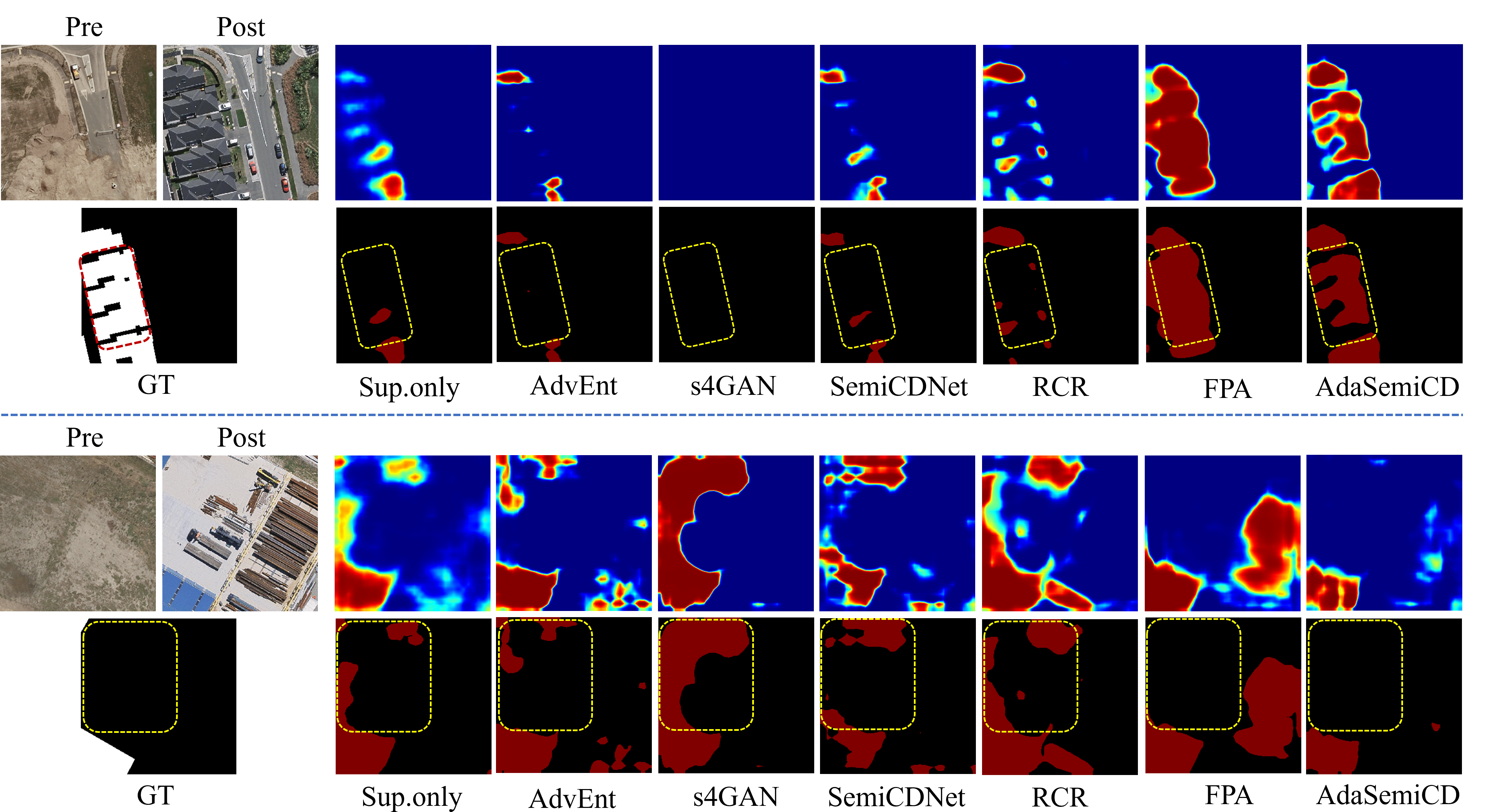
Figure 4: Visualizations of different models on the WHU-CD dataset. Pre and Post represent the image of the front and back temporal respectively, and GT is the Ground Truth.

IV-C Ablation study

In this section, we conduct some ablation studies, mainly to verify the role of each module in our proposed approach and to explore some of our hyperparameter selections in the experiment.

Effectiveness of proposed modules: Due to the differences in model architecture between the current semi-supervised change detection methods referred to and ours, we did not rush to verify the superiority of our method at first. Instead, we conducted model architecture experiments first, using the classical Mean-Teacher architecture. In addition to setting hyperparameters for it to control the weight of unsupervised losses, the rest of the data augmentations and CD network remained the same as [27] and [25]. The gain of this semi-supervised framework compared with the single model and the two-branch network with shared weights is very obvious, and it can almost approach the previous optimal performance. This also demonstrates the validity of the principle of perturbed consistency and the parameter integration, on the basis of which we explore the adaptive training mechanism. Therefore, we separately integrated our proposed AdaEMA and AdaFusion into the MT framework and achieved average improvement of 1.2 and 5.1 on $IoU^{c}$ respectively, as shown in Table IV. * in the table indicates that in adapt, an adaptive judgment operation is performed to determine whether the fusion is performed, and a random selection strategy is used when selecting the fusion region, and a huge gap between the two is evident. Finally, the two adaptive modules contain the complete method, and better results are obtained on the basis of individual modules, which shows that the two modules proposed by us are decoupled, and the model architecture is reasonable.

TABLE IV: Ablation study of our proposed AdaSemiCD on LEVIR-CD Dataset. AEMA and AF denotes our AdaEMA, AdaFusion module respectively. And AF* represents the fusion region are randomly selected.

Method	5%			10%			20%			40%
	$IoU^{c}$	OA		$IoU^{c}$	OA		$IoU^{c}$	OA		$IoU^{c}$	OA
Sup. only	61.0	97.60		66.8	98.13		72.3	98.44		74.9	98.60
MT-EMA	67.1 (+6.1)	98.14 (+0.54)		75.0 (+8.2)	98.63 (+0.50)		76.6 (+4.3)	98.71 (+0.27)		77.0 (+2.1)	98.73 (+0.13)
MT-AEMA	68.9 (+7.9)	98.23 (+0.63)		76.1 (+9.3)	98.66 (+0.53)		77.7 (+5.4)	98.78 (+0.34)		77.8 (+2.9)	98.78 (+0.18)
(MT-EMA)+AF*	72.0 (+11.0)	98.43 (+0.83)		76.8 (+10.0)	98.72 (+0.59)		77.5 (+5.2)	98.74 (+0.30)		78.5 (+3.6)	98.80 (+0.20)
(MT-EMA)+AF	77.0 (+16.0)	98.72 (+1.12)		78.8 (+12.0)	98.83 (+0.70)		80.4 (+8.1)	98.91 (+0.47)		80.0 (+5.1)	98.90 (+0.30)
AdaSemiCD	77.7 (+16.7)	98.78 (+1.18)		79.4 (+12.6)	98.87 (+0.74)		80.3 (+8.0)	98.92 (+0.48)		80.6 (+5.7)	98.93 (+0.33)

Hyperparameters in Ramp-up: The Ramp-up process has a significant influence on the performance of our AdaSemiCD on SSCD. Therefore, we conduct experiments on the selection of two hyperparameters ($\gamma$ and $w_{max}$) a and b that control the Ramp-up process. As shown in Table V, our method achieves the best performance on the three datasets under the combination of parameters (0.1, 10), (0.1, 0.1), and (0.1, 1.0) respectively. Moreover, our method is sensitive to this hyperparameter, and inappropriate parameter selection will cause large performance attenuation. This is because our method conducts supervised training on labeled samples and unsupervised training on unlabeled samples at the same time. If the relationship between the two cannot be properly balanced, overfitting on labeled samples or excessive noise interference from unlabeled samples will be caused. All of our remaining experiments were performed at this hyperparameter setting, and the hyperparameters of the compared methods were consistent with the best choices in their original paper.

TABLE V: Sensitivity analysis of ramp-up hyperparameters with 10$\%$ labeled data on the LEVIR-CD, WHU-CD, and CDD datasets.

$\gamma$	$w_{max}$	LEVIR-CD			WHU-CD			CDD
		$IoU^{c}$	OA		$IoU^{c}$	OA		$IoU^{c}$	OA
0	0 (Sup.Only)	66.8	98.13		55.7	97.53		67.9	95.46
0.05	1.0	67.2	98.17		53.8	97.02		74.4	96.35
0.1	1.0	71.8	98.32		61.0	98.10		77.3	96.89
0.3	1.0	69.9	98.26		59.4	98.03		76.2	96.56
0.5	1.0	68.7	98.15		60.9	98.25		76.3	96.58
1.0	1.0	67.3	98.13		60.5	98.18		72.3	95.98
0.1	0.1	65.2	97.60		70.8	98.70		71.6	95.77
0.1	0.5	68.3	98.14		66.9	98.54		75.8	96.67
0.1	5.0	73.9	98.75		60.1	98.00		69.1	95.51
0.1	10.0	79.4	98.87		52.4	97.40		68.2	95.50
0.1	30.0	71.9	98.42		50.34	97.12		65.4	95.20

IV-D Complexity Analysis

Since we utilize the same architecture with FPA and RCR, the number of training parameters (46.85M) and computational amount (585.85 GFLOPs) were the same. The variations in parameters, FLOPs, and the time required for training and inference are presented in Table VI. Our AdaSemiCD is comparable to other methods with reference count, FLOPs, and inference time. The main reason for the longer training time was that it took about 0.3s for each iteration to generate and evaluate pseudo-labels twice, while it only took about 0.006s and 0.03s for fusion and EMA parameters updating, respectively. Moreover, our model balances performance and time consumption, offering a notable performance benefit with only a slight increase in time.

TABLE VI: COMPARISON OF PARAMETERS, COMPUTING COMPLEXITY, AND TRAINING TIME OF DIFFERENT SSCD METHODS ON 5$\%$ LABELED LEVIR-CD Dataset.

Method	Params(M)	FLOPs(G)	Training Time(s)	Inference Time(ms)	$IoU^{c}$
Sup.Only	46.85	585.85	77	56	61.0
AdvEnt[68]	46.85	585.85	405	63	66.1
s4GAN[37]	46.85	585.85	585	58	64.0
SemiCDNet[26]	46.85	585.85	408	75	67.6
RCR[25]	46.85	585.85	742	59	72.5
FPA[27]	46.85	585.85	727	68	73.7
AdaSemiCD	46.85	585.85	915	67	77.7
Oracle	46.85	585.85	293	55	77.9

IV-E Limitation Analysis and Future Work

Although our approach is effective in most scenarios, we also found in our experiments that there are certain limitations in some cases. As shown in Fig. 5, our approach struggled and even performed worse than the supervised approach when faced with the detection of areas of leptosomatic variation, such as highways, rivers, and so on, especially from the example in the upper right corner, it can be seen that our method has great advantages in the identification and detection of blocky change areas. This is because when our AdaFusion transforms samples, it is the fusion of patch to patch, which easily truncates this changing region that throughout the entire image, and there is too little real data with annotations, resulting in no effective knowledge to be learned.

Therefore, in future research work, more targeted fusion methods could designed to avoid such information loss. For example, a changing region is regarded as an instance and sample fusion is carried out at the instance level. In this way, the characteristics of different change types can be preserved to a great extent while noise is removed, additional supervisory information is introduced and sample diversity is expanded. We will also actively explore the application of this adaptive mechanism to other semi-supervised tasks and frameworks.

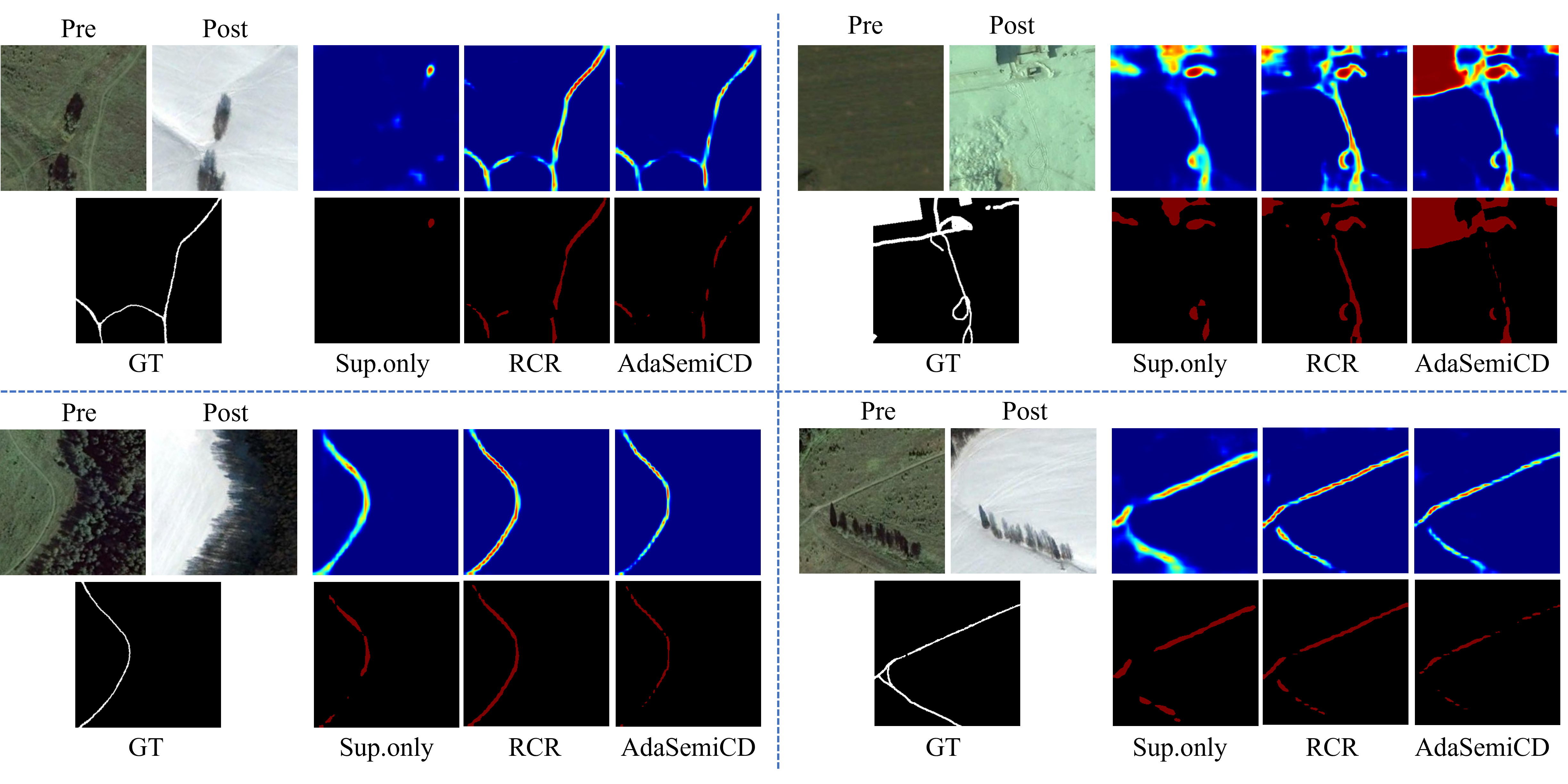
Figure 5: Examples of common error cases in the CDD dataset.

V Conclusion

In this study, we present AdaSemiCD, a flexible semi-supervised framework for change detection. This framework assesses the quality of pseudo-labels on unlabeled training samples and implements adaptive modifications based on the assessment outcomes, which include sample fusion (AdaFusion), and parameter updates (AdaEMA). Despite the complexity of the scenes, our model successfully identifies the areas of interest with minimal interference during training. Empirical evidence from several publicly available CD datasets attests to the efficacy of our methodology. Looking ahead, this adaptive processing technique holds promise for potential application in other semi-supervised tasks.

References

- [1] X. Zhang, Y. Yang, L. Ran, L. Chen, K. Wang, L. Yu, P. Wang, and Y. Zhang, “Remote sensing image semantic change detection boosted by semi-supervised contrastive learning of semantic segmentation,” IEEE Transactions on Geoscience and Remote Sensing, vol. 62, pp. 1–13, 2024.
- [2] M. Bouziani, K. Goïta, and D.-C. He, “Automatic change detection of buildings in urban environment from very high spatial resolution images using existing geodatabase and prior knowledge,” ISPRS Journal of Photogrammetry and Remote Sensing, vol. 65, no. 1, pp. 143–153, 2010.
- [3] Y. Xing, Q. Zhang, L. Ran, X. Zhang, H. Yin, and Y. Zhang, “Progressive modality-alignment for unsupervised heterogeneous change detection,” IEEE Transactions on Geoscience and Remote Sensing, vol. 61, pp. 1–12, 2023.
- [4] ——, “Improving reliability of heterogeneous change detection by sample synthesis and knowledge transfer,” IEEE Transactions on Geoscience and Remote Sensing, vol. 62, pp. 1–11, 2024.
- [5] R. Anniballe, F. Noto, T. Scalia, C. Bignami, S. Stramondo, M. Chini, and N. Pierdicca, “Earthquake damage mapping: An overall assessment of ground surveys and vhr image change detection after l’aquila 2009 earthquake,” Remote sensing of environment, vol. 210, pp. 166–178, 2018.
- [6] Z. Y. Lv, W. Shi, X. Zhang, and J. A. Benediktsson, “Landslide inventory mapping from bitemporal high-resolution remote sensing images using change detection and multiscale segmentation,” IEEE Journal of Selected Topics in Applied Earth Observations and Remote Sensing, vol. 11, no. 5, pp. 1520–1532, 2018.
- [7] R. Caye Daudt, B. Le Saux, and A. Boulch, “Fully Convolutional Siamese Networks for Change Detection,” in 2018 25th IEEE International Conference on Image Processing (ICIP). IEEE, 2018, pp. 4063–4067.
- [8] H. Zhang, H. Chen, C. Zhou, K. Chen, C. Liu, Z. Zou, and Z. Shi, “Bifa: Remote sensing image change detection with bitemporal feature alignment,” IEEE Transactions on Geoscience and Remote Sensing, vol. 62, pp. 1–17, 2024.
- [9] H. Chen, H. Zhang, K. Chen, C. Zhou, S. Chen, Z. Zou, and Z. Shi, “Continuous cross-resolution remote sensing image change detection,” IEEE Transactions on Geoscience and Remote Sensing, vol. 61, pp. 1–20, 2023.
- [10] H. Chen, Z. Qi, and Z. Shi, “Remote sensing image change detection with transformers,” IEEE Transactions on Geoscience and Remote Sensing, vol. 60, pp. 1–14, 2022.
- [11] W. G. C. Bandara and V. M. Patel, “A transformer-based siamese network for change detection,” in IGARSS 2022 - 2022 IEEE International Geoscience and Remote Sensing Symposium, 2022, pp. 207–210.
- [12] Z. Zheng, Y. Zhong, S. Tian, A. Ma, and L. Zhang, “Changemask: Deep multi-task encoder-transformer-decoder architecture for semantic change detection,” ISPRS Journal of Photogrammetry and Remote Sensing, vol. 183, pp. 228–239, Jan. 2022.
- [13] H. Chen, Y. Zao, L. Liu, S. Chen, and Z. Shi, “Semantic decoupled representation learning for remote sensing image change detection,” in IGARSS 2022 - 2022 IEEE International Geoscience and Remote Sensing Symposium, 2022, pp. 1051–1054.
- [14] H. Chen, W. Li, S. Chen, and Z. Shi, “Semantic-aware dense representation learning for remote sensing image change detection,” IEEE Transactions on Geoscience and Remote Sensing, vol. 60, pp. 1–18, 2022.
- [15] L. Yan, J. Yang, and J. Wang, “Domain knowledge-guided self-supervised change detection for remote sensing images,” IEEE Journal of Selected Topics in Applied Earth Observations and Remote Sensing, vol. 16, pp. 4167–4179, 2023.
- [16] W. G. C. Bandara and V. M. Patel, “Deep metric learning for unsupervised remote sensing change detection,” arXiv preprint arXiv:2303.09536, 2023.
- [17] X. Tang, H. Zhang, L. Mou, F. Liu, X. Zhang, X. X. Zhu, and L. Jiao, “An unsupervised remote sensing change detection method based on multiscale graph convolutional network and metric learning,” IEEE Transactions on Geoscience and Remote Sensing, vol. 60, pp. 1–15, 2022.
- [18] C. Wu, B. Du, and L. Zhang, “Fully convolutional change detection framework with generative adversarial network for unsupervised, weakly supervised and regional supervised change detection,” IEEE Transactions on Pattern Analysis and Machine Intelligence, vol. 45, no. 8, pp. 9774–9788, 2023.
- [19] Z. Li, C. Tang, X. Liu, C. Li, X. Li, and W. Zhang, “Ms-former: Memory-supported transformer for weakly supervised change detection with patch-level annotations,” IEEE Transactions on Geoscience and Remote Sensing, vol. 62, pp. 1–13, 2024.
- [20] L. Ma, Y. Huang, W. Shi, Y. Wang, and X. Ye, “Weakly supervised building change detection based on deepcut and temporal invariant,” IEEE Transactions on Geoscience and Remote Sensing, vol. 62, pp. 1–18, 2024.
- [21] H. Chen, W. Li, and Z. Shi, “Adversarial instance augmentation for building change detection in remote sensing images,” IEEE Transactions on Geoscience and Remote Sensing, vol. 60, pp. 1–16, 2022.
- [22] C. Ren, X. Wang, J. Gao, X. Zhou, and H. Chen, “Unsupervised change detection in satellite images with generative adversarial network,” IEEE Transactions on Geoscience and Remote Sensing, vol. 59, no. 12, pp. 10 047–10 061, 2021.
- [23] Z. Wang, D. Liu, Z. Wang, X. Liao, and Q. Zhang, “A new remote sensing change detection data augmentation method based on mosaic simulation and haze image simulation,” IEEE Journal of Selected Topics in Applied Earth Observations and Remote Sensing, vol. 16, pp. 4579–4590, 2023.
- [24] W. G. C. Bandara, N. G. Nair, and V. M. Patel, “Ddpm-cd: Remote sensing change detection using denoising diffusion probabilistic models,” arXiv preprint arXiv:2206.11892, 2022.
- [25] W. G. C. Bandara and V. M. Patel, “Revisiting consistency regularization for semi-supervised change detection in remote sensing images,” arXiv preprint arXiv:2204.08454, 2022.
- [26] D. Peng, L. Bruzzone, Y. Zhang, H. Guan, H. Ding, and X. Huang, “Semicdnet: A semisupervised convolutional neural network for change detection in high resolution remote-sensing images,” IEEE Transactions on Geoscience and Remote Sensing, vol. 59, no. 7, pp. 5891–5906, Jul. 2021.
- [27] X. Zhang, X. Huang, and J. Li, “Semisupervised change detection with feature-prediction alignment,” IEEE Transactions on Geoscience and Remote Sensing, vol. 61, pp. 1–16, 2023.
- [28] L. Ran, W. Zhan, Y. Li, X. Zhang, and S. Zhang, “Dtfseg: A dynamic threshold filtering method for semi-supervised semantic segmentation,” in 2023 China Automation Congress (CAC). Chongqing, China: IEEE, Nov. 2023, pp. 7571–7576.
- [29] L. Ran, L. Wang, T. Zhuo, Y. Xing, and Y. Zhang, “Ddf: A novel dual-domain image fusion strategy for remote sensing image semantic segmentation with unsupervised domain adaptation,” IEEE Transactions on Geoscience and Remote Sensing, vol. 62, pp. 1–13, 2024.
- [30] L. Ran, Y. Li, G. Liang, and Y. Zhang, “Semi-supervised semantic segmentation based on pseudo-labels: A survey,” arXiv preprint arXiv:2403.01909, 2024.
- [31] S. Yuan, R. Zhong, C. Yang, Q. Li, and Y. Dong, “Dynamically updated semi-supervised change detection network combining cross-supervision and screening algorithms,” IEEE Transactions on Geoscience and Remote Sensing, vol. 62, pp. 1–14, 2024.
- [32] A. Tarvainen and H. Valpola, “Mean teachers are better role models: Weight-averaged consistency targets improve semi-supervised deep learning results,” Advances in neural information processing systems, vol. 30, 2017.
- [33] Z. Zhao, L. Yang, S. Long, J. Pi, L. Zhou, and J. Wang, “Augmentation matters: A simple-yet-effective approach to semi-supervised semantic segmentation,” in Proceedings of the IEEE/CVF conference on computer vision and pattern recognition, 2023, pp. 11 350–11 359.
- [34] S. Yun, D. Han, S. J. Oh, S. Chun, J. Choe, and Y. Yoo, “Cutmix: Regularization strategy to train strong classifiers with localizable features,” in Proceedings of the IEEE/CVF international conference on computer vision, 2019, pp. 6023–6032.
- [35] S. Laine and T. Aila, “Temporal ensembling for semi-supervised learning,” in 5th International Conference on Learning Representations, ICLR, 2017.
- [36] P. Mi, J. Lin, Y. Zhou, Y. Shen, G. Luo, X. Sun, L. Cao, R. Fu, Q. Xu, and R. Ji, “Active teacher for semi-supervised object detection,” in Proceedings of the IEEE/CVF conference on computer vision and pattern recognition, 2022, pp. 14 482–14 491.
- [37] S. Mittal, M. Tatarchenko, and T. Brox, “Semi-supervised semantic segmentation with high-and low-level consistency,” IEEE transactions on pattern analysis and machine intelligence, vol. 43, no. 4, pp. 1369–1379, 2019.
- [38] L. Yang, L. Qi, L. Feng, W. Zhang, and Y. Shi, “Revisiting weak-to-strong consistency in semi-supervised semantic segmentation,” in Proceedings of the IEEE/CVF Conference on Computer Vision and Pattern Recognition, 2023, pp. 7236–7246.
- [39] Z. Zhao, S. Long, J. Pi, J. Wang, and L. Zhou, “Instance-specific and model-adaptive supervision for semi-supervised semantic segmentation,” in Proceedings of the IEEE/CVF conference on computer vision and pattern recognition, 2023, pp. 23 705–23 714.
- [40] K. Sohn, D. Berthelot, N. Carlini, Z. Zhang, H. Zhang, C. A. Raffel, E. D. Cubuk, A. Kurakin, and C.-L. Li, “Fixmatch: Simplifying semi-supervised learning with consistency and confidence,” Advances in neural information processing systems, vol. 33, pp. 596–608, 2020.
- [41] X. Li, L. Yu, H. Chen, C.-W. Fu, L. Xing, and P.-A. Heng, “Transformation-consistent self-ensembling model for semisupervised medical image segmentation,” IEEE transactions on neural networks and learning systems, vol. 32, no. 2, pp. 523–534, 2020.
- [42] Y. Zhang, Y. Cheng, and Y. Qi, “Semisam: Exploring sam for enhancing semi-supervised medical image segmentation with extremely limited annotations,” arXiv preprint arXiv:2312.06316, 2023.
- [43] Q. Xie, Z. Dai, E. Hovy, T. Luong, and Q. Le, “Unsupervised data augmentation for consistency training,” Advances in neural information processing systems, vol. 33, pp. 6256–6268, 2020.
- [44] X. Lai, Z. Tian, L. Jiang, S. Liu, H. Zhao, L. Wang, and J. Jia, “Semi-supervised semantic segmentation with directional context-aware consistency,” in Proceedings of the IEEE/CVF Conference on Computer Vision and Pattern Recognition, 2021, pp. 1205–1214.
- [45] L. Yang, W. Zhuo, L. Qi, Y. Shi, and Y. Gao, “St++: Make self-training work better for semi-supervised semantic segmentation,” in Proceedings of the IEEE/CVF conference on computer vision and pattern recognition, 2022, pp. 4268–4277.
- [46] Y. Wang, H. Wang, Y. Shen, J. Fei, W. Li, G. Jin, L. Wu, R. Zhao, and X. Le, “Semi-supervised semantic segmentation using unreliable pseudo-labels,” in Proceedings of the IEEE/CVF conference on computer vision and pattern recognition, 2022, pp. 4248–4257.
- [47] E. Bousias Alexakis and C. Armenakis, “Evaluation of semi-supervised learning for cnn-based change detection,” The International Archives of the Photogrammetry, Remote Sensing and Spatial Information Sciences, vol. 43, pp. 829–836, 2021.
- [48] Z. Mao, X. Tong, and Z. Luo, “Semi-supervised remote sensing image change detection using mean teacher model for constructing pseudo-labels,” in ICASSP 2023 - 2023 IEEE International Conference on Acoustics, Speech and Signal Processing (ICASSP), 2023, pp. 1–5.
- [49] C. Sun, J. Wu, H. Chen, and C. Du, “Semisanet: A semi-supervised high-resolution remote sensing image change detection model using siamese networks with graph attention,” Remote Sensing, vol. 14, no. 12, p. 2801, 2022.
- [50] S. Hafner, Y. Ban, and A. Nascetti, “Urban change detection using a dual-task siamese network and semi-supervised learning,” in IGARSS 2022 - 2022 IEEE International Geoscience and Remote Sensing Symposium, 2022, pp. 1071–1074.
- [51] I. Goodfellow, J. Pouget-Abadie, M. Mirza, B. Xu, D. Warde-Farley, S. Ozair, A. Courville, and Y. Bengio, “Generative adversarial nets,” Advances in neural information processing systems, vol. 27, 2014.
- [52] J. Liu, K. Chen, G. Xu, H. Li, M. Yan, W. Diao, and X. Sun, “Semi-supervised change detection based on graphs with generative adversarial networks,” in IGARSS 2019-2019 IEEE International Geoscience and Remote Sensing Symposium. IEEE, 2019, pp. 74–77.
- [53] W. Nie, P. Gou, Y. Liu, B. Shrestha, T. Zhou, N. Xu, P. Wang, and Q. Du, “Semi supervised change detection method of remote sensing image,” in 2022 IEEE 6th Advanced Information Technology, Electronic and Automation Control Conference (IAEAC). IEEE, 2022, pp. 1013–1019.
- [54] S. Yang, S. Hou, Y. Zhang, H. Wang, and X. Ma, “Change detection of high-resolution remote sensing image based on semi-supervised segmentation and adversarial learning,” in IGARSS 2022-2022 IEEE International Geoscience and Remote Sensing Symposium. IEEE, 2022, pp. 1055–1058.
- [55] C. Ren, X. Wang, J. Gao, X. Zhou, and H. Chen, “Unsupervised change detection in satellite images with generative adversarial network,” IEEE Transactions on Geoscience and Remote Sensing, vol. 59, no. 12, pp. 10 047–10 061, 2020.
- [56] Y. Li, H. Chen, S. Dong, Y. Zhuang, and L. Li, “Multi-temporal samplepair generation for building change detection promotion in optical remote sensing domain based on generative adversarial network,” Remote Sensing, vol. 15, no. 9, p. 2470, 2023.
- [57] J. G. Vinholi, P. R. B. d. Silva, D. I. Alves, and R. Machado, “Enhancing change detection in ultra-wideband vhf sar imagery: An entropy-based approach with median ground scene masking,” IEEE Transactions on Geoscience and Remote Sensing, vol. 62, pp. 1–15, 2024.
- [58] J. Zhang, Z. Shao, Q. Ding, X. Huang, Y. Wang, X. Zhou, and D. Li, “Aernet: An attention-guided edge refinement network and a dataset for remote sensing building change detection,” IEEE Transactions on Geoscience and Remote Sensing, vol. 61, pp. 1–16, 2023.
- [59] H. Chen and Z. Shi, “A spatial-temporal attention-based method and a new dataset for remote sensing image change detection,” Remote Sensing, vol. 12, no. 10, p. 1662, 2020.
- [60] S. Ji, S. Wei, and M. Lu, “Fully convolutional networks for multisource building extraction from an open aerial and satellite imagery data set,” IEEE Transactions on geoscience and remote sensing, vol. 57, no. 1, pp. 574–586, 2018.
- [61] S. Holail, T. Saleh, X. Xiao, and D. Li, “Afde-net: Building change detection using attention-based feature differential enhancement for satellite imagery,” IEEE Geoscience and Remote Sensing Letters, vol. 20, pp. 1–5, 2023.
- [62] M. Liu, Z. Chai, H. Deng, and R. Liu, “A cnn-transformer network with multiscale context aggregation for fine-grained cropland change detection,” IEEE Journal of Selected Topics in Applied Earth Observations and Remote Sensing, vol. 15, pp. 4297–4306, 2022.
- [63] M. Lebedev, Y. V. Vizilter, O. Vygolov, V. A. Knyaz, and A. Y. Rubis, “Change detection in remote sensing images using conditional adversarial networks,” The International Archives of the Photogrammetry, Remote Sensing and Spatial Information Sciences, vol. 42, pp. 565–571, 2018.
- [64] Q. Shi, M. Liu, S. Li, X. Liu, F. Wang, and L. Zhang, “A deeply supervised attention metric-based network and an open aerial image dataset for remote sensing change detection,” IEEE Transactions on Geoscience and Remote Sensing, vol. 60, pp. 1–16, 2022.
- [65] C. Zhang, P. Yue, D. Tapete, L. Jiang, B. Shangguan, L. Huang, and G. Liu, “A deeply supervised image fusion network for change detection in high resolution bi-temporal remote sensing images,” ISPRS Journal of Photogrammetry and Remote Sensing, vol. 166, pp. 183–200, 2020.
- [66] H. Zhang, M. Cisse, Y. N. Dauphin, and D. Lopez-Paz, “mixup: Beyond empirical risk minimization,” arXiv preprint arXiv:1710.09412, 2017.
- [67] E. D. Cubuk, B. Zoph, J. Shlens, and Q. V. Le, “Randaugment: Practical automated data augmentation with a reduced search space,” in Proceedings of the IEEE/CVF conference on computer vision and pattern recognition workshops, 2020, pp. 702–703.
- [68] T.-H. Vu, H. Jain, M. Bucher, M. Cord, and P. Pérez, “Advent: Adversarial entropy minimization for domain adaptation in semantic segmentation,” in Proceedings of the IEEE/CVF conference on computer vision and pattern recognition, 2019, pp. 2517–2526.