Generative Feature Training of Thin 2-Layer Networks
Abstract
We consider the approximation of functions by 2-layer neural networks with a small number of hidden weights based on the squared loss and small datasets. Due to the highly non-convex energy landscape, gradient-based training often suffers from local minima. As a remedy, we initialize the hidden weights with samples from a learned proposal distribution, which we parameterize as a deep generative model. To train this model, we exploit the fact that with fixed hidden weights, the optimal output weights solve a linear equation. After learning the generative model, we refine the sampled weights with a gradient-based post-processing in the latent space. Here, we also include a regularization scheme to counteract potential noise. Finally, we demonstrate the effectiveness of our approach by numerical examples.
1 Introduction
We investigate the approximation of real-valued functions . To this end, assume that we are given samples , where are independently drawn from some distribution and are possibly noisy observations of . For approximating based on , we study parametric architectures of the form
| (1) |
where denotes the real part, is a nonlinear function, and are the features with corresponding weights . If the function is real-valued, the model (1) simplifies to a standard 2-layer neural network architecture without and with . The more general model (1) also covers other frameworks such as random Fourier features (Rahimi & Recht, 2007).
For a fixed activation function and width , we aim to find parameters such that the from (1) approximates well. From a theoretical perspective, we can minimize the mean squared error (MSE), namely
| (2) |
to obtain the parameters . In practice, however, we do not have direct access to and , but only to data points , where are iid samples from and are noisy versions of . Hence, we replace (2) by the empirical risk minimization
| (3) |
However, if is small, minimizing (3) can lead to significant overfitting towards the training samples and poor generalization. To circumvent this problem, we investigate the following principles.
-
•
We use architectures of the form (1) with small . This amounts to the implicit assumption that can be sparsely represented with this model. Unfortunately, such under-parameterized networks () are difficult to train with conventional gradient-based algorithms (Boob et al., 2022; Holzmüller & Steinwart, 2022), see also Table 1. Hence, we require an alternative training strategy.
-
•
Often, we have prior information about the regularity of , i.e., that is in some Banach space with a norm of the form
(4) where is some differential operator and . A common example within this framework is the space of bounded variation (Ambrosio et al., 2000), which informally corresponds to the choice , and . In practice, the integral in (4) is often approximated using Monte Carlo methods with uniformly distributed samples . If we use (4) as regularizer for , the generalization error can be analyzed in Barron spaces (Li et al., 2022).
Contribution
We propose a generative modeling approach to solve (3). To this end, we first observe that the minimization with respect to is a linear least squares problem. Based on this, we analytically express the optimal in terms of , which leads to a reduced problem. Using the implicit function theorem, we can compute and hence the gradient of the reduced objective. To facilitate its optimization, we replace the deterministic features with stochastic ones, and optimize over their underlying distribution instead. We parameterize this distribution as with a deep network . Hence, we coin our approach as generative feature training. Further, we propose to add a Monte Carlo approximation of the norm (4) to the reduced objective. With this regularization, we aim to prevent overfitting.
2 Related Work
Random Features
Random feature models (RFM) first appeared in the context of kernel approximation (Rahimi & Recht, 2007; Liu et al., 2021), which enables the fast computation of large kernel sums with certain error bounds, see also Rahimi & Recht (2008); Cortes et al. (2010); Rudi & Rosasco (2017). Representations of the form (1) with only a few active features, so-called sparse random features (Yen et al., 2014), can be computed based on basis pursuit (Hashemi et al., 2023). Since this often leads to suboptimal approximation accuracy, later works by Bai et al. (2024); Xie et al. (2022); Saha et al. (2023) instead proposed to apply pruning or hard-thresholding algorithms to reduce the size of the feature set. Commonly, the features are sampled from Gaussian mixtures with diagonal covariances. For adapting these to the data, Potts & Schmischke (2021); Potts & Weidensager (2024) propose to identify the relevant subspaces for the feature proposal based on the ANOVA decomposition. Such features with only a few non-zero entries also enable a fast evaluation of the representation (1) via the non-equispaced fast Fourier transform (Dutt & Rokhlin, 1993; Potts et al., 2001). For kernel approximations, this can be also achieved with slicing methods (Hertrich, 2024; Hertrich et al., 2024), which are again closely related to random feature models (Rux et al., 2024).
Adaptive Features
There are also other attempts to design data-adapted proposal distributions for random features (Li et al., 2019b). More recently, Bolager et al. (2023) proposed to only sample the features in regions where it matters, i.e., based on the available gradient information. While this allows some adaption, the still remain fixed after sampling them (a so-called greedy approach). Towards fully adaptive (Fourier) features , Li et al. (2019a) propose to alternately solve for the optimal , and to then perform a gradient update for the . Kammonen et al. (2020) propose to instead update the based on some Markov Chain Monte Carlo method. While both methods update the proposal distribution , they do not embed the linear least squares problem into this step. It is well known that such alternating updates can perform poorly in certain instances. Note that learnable features have been also used in the context of positional encoding (Li et al., 2021).
2-Layer ReLU Networks
We can interpret 2-layer neural networks as adaptive kernel methods (E et al., 2019). Moreover, they have essentially the same generalization error as the random feature model. Several works investigate the learning of the architecture (1) with based on a (modified) version of the empirical risk minimization (3). Based on convex duality, Pilanci & Ergen (2020) derive a semi-definite program to find a global minimizer of (3). A huge drawback is that this method scales exponentially in the dimension . Later, several accelerations based on convex optimization algorithms have been proposed (Bai et al., 2023; Mishkin et al., 2022). Following a different approach, Barbu (2023) proposed to use an alternating minimization over the parameters and that keeps the activation pattern fixed throughout the training. While this has an improved complexity of in the dimension , the approach is still restricted to ReLU-like functions . A discussion of the rich literature on global minimization guarantees in the over-parameterized regime () is not within the scope of this paper.
Bayesian Networks
Another approach that samples neural network weights is Bayesian neural networks (BNNs) (Neal, 2012; Jospin et al., 2022). This allows to capture the uncertainty on the weights in overparameterized architectures. A fundamental difference to our approach and random feature models is that we sample the features independently from the same distribution, while BNNs usually learn a separate one for each . Further, BNNs are usually trained by minimizing an evidence lower bound instead of (8), see for example (Graves, 2011; Blundell et al., 2015), which is required to prevent collapsing distributions.
3 Generative Feature Learning
Given data points with for some underlying function , we aim to find the optimal features and corresponding weights such that , where the approximator is defined in (1). Before we introduce our learning scheme for the parameters and , we discuss two important choices of the nonlinearity that appear in the literature.
Example 1.
-
i)
Fourier Features: The choice is reasonable if the ground-truth function can be represented by few Fourier features, e.g., if it is smooth. As discussed in Section 2, the deployed features are commonly selected by randomized pruning algorithms.
-
ii)
2-Layer Neural Network: For , we can restrict ourselves to . Common examples are the ReLU and the sigmoid . Then, corresponds to a 2-layer neural network (i.e., with one hidden layer). Using the so-called bias trick, we can include a bias into (1). That is, we use padded data-points such that the last entry of the feature vectors can act as bias. Similarly, an output bias can be included by padding the hidden layer output with some constant value.
In the following, we outline our training procedure for optimizing the parameters and in . As first step, we derive an analytic formula for the optimal weights in the empirical risk minimization (3) with fixed features . Then, in the spirit of random Fourier features, we propose to sample the from a proposal distribution , which we learn based on the generative modeling ansatz . As last step, we fine-tune the sampled features by updating the sampled latent features with the Adam optimizer. In order to be able to deal with noisy function values , we can regularize the approximation during training. Our complete approach is summarized in Algorithm 1.
3.1 Computing the Optimal Weights
For fixed , any optimal weights for (3) solves the linear system
| (5) |
where and . In order to stabilize the numerical solution of (5), we deploy Tikhonov regularization with small regularization strength , and instead compute as the unique solution of
| (6) |
A key aspect of our approach is that we can compute using the implicit function theorem. This requires solving another linear equation of the form (6) with a different right hand side. For small , the most efficient approach for solving (6) is to use a LU decomposition, and to reuse the obtained decomposition for the backward pass. This procedure is readily implemented in many AD packages such as PyTorch, and no additional coding is required.
Now, by inserting the solution of (6) into the empirical loss (3), we obtain the reduced loss
| (7) |
Naively, we can try to minimize (7) directly via a gradient-based iterative method (such as Adam with its default parameters) starting at some random initialization . However, is non-convex, and our comparisons in Section 4 reveal that the optimization frequently gets stuck in local minima. Consequently, a good initialization is crucial if we want to minimize (7) with a gradient-based method. In the spirit of random Fourier features, we propose to initialize the features as independent identically distributed (iid) samples from a proposal distribution . To the best of our knowledge, current random Fourier feature methods all rely on a handcrafted .
3.2 Learning the Proposal Distribution
Since the optimal is in general not expressible without knowledge of , we aim to learn it from the available data based on a generative model. That is, we take a simple latent distribution (such as the normal distribution ) and make the parametric ansatz . Here, is a fully connected neural network with parameters and denotes the push-forward of under . To optimize the parameters of the distribution , we minimize the expectation of the reduced loss (7) with iid features sampled from , namely the loss
| (8) |
The loss (8) can now be minimized by a stochastic gradient-based algorithm. That is, in each step, we sample one realization of the latent features to get an estimate for the expectation in (8). Then, we compute the gradient of the integrand with respect to for this specific , and update with our chosen optimizer. In the following, we provide some intuition why this approach outperforms standard training approaches. At the beginning of the training, most of the randomly sampled features do not fit to the data. Hence, they will suffer from vanishing gradients and be updated only slowly. On the other hand, since the stochastic generator leads to an evaluation of the objective at many different locations, we quickly gather gradient information for a large variety of features locations. In particular, always taking fresh samples from the iteratively updated proposal distribution helps to efficiently get rid of useless features.
3.3 Feature Refinement: Adam in the Latent Space
Once the feature distribution is learned, we sample a collection of iid latent features . By design, the associated features (with being applied elementwise to ) serve as an estimate for a minimizer of (7). This estimate is now fine-tuned with the Adam optimizer. That is, starting in , we minimize the function
| (9) |
where is the loss function from (7). By noting that , this corresponds to initializing the Adam optimizer for the function with , and to additionally precondition it by the Jacobian matrix of the generator . If the step size is chosen appropriately, we expect that the value of will decrease with the iterations. Conceptually, our refinement approach is similar to many second-order optimization routines, which also require a good initialization for convergence.
3.4 Regularization for Noisy Data
If the number of training points is small or if the noise on the values is strong, the minimization of the empirical risk (3) can suffer from overfitting (i.e., the usage of high-frequency features). In order to prevent this, we can deploy a regularizer of the form (4). This leads to the regularized training problem
| (10) |
with . We choose the parameters in (10) as , and , which leads to the (anisotropic) total variation regularizer (Acar & Vogel, 1994; Chan & Esedoglu, 2005). More precisely, we get
| (11) |
where is the uniform distribution on , where and are the entry-wise minimum and maximum of the training data. For our generative training formulation (8), adding (11) leads to the problem
| (12) |
Similarly, we replace the from (9) by
| (13) |
for the feature refinement in the latent space. If we have more specific knowledge about the function that we try to approximate, then we can also apply more restrictive regularizers of the form (10). As discussed in Section 2, several random feature methods instead regularize the feature selection by incorporating sparsity of the feature vectors , namely that they only have a few non-zero entries.
4 Experiments
We demonstrate the effectiveness of our method with three numerical examples. First, we visually inspect the obtained features. Here, we also check if they recover the correct subspaces. Secondly, we benchmark our methods on common test functions from approximation theory, i.e., with a known groundtruth. Lastly, we target regression on some datasets from the UCI database.
4.1 Setup and Comparisons
For all experiments, we deploy the architecture in (1) with features and one of the functions from Example 1:
-
•
We deploy without the bias trick. This corresponds to the approximation of the underlying ground truth function by Fourier features.
-
•
We deploy , which corresponds to a 2-layer network with sigmoid activation functions. To improve the expressiveness of the model, we apply the bias trick for both layers.
Further, we choose the generator for the proposal distribution as ReLU network with 3 hidden layers and 512 neurons per hidden layer. It remains to pick the regularization strength . For this, we divide the original training data into a training (90%) and a validation (10%) set. Then, we train for each and choose the with the best validation error. To minimize the involved regularized loss functions (proposal distribution, see also (12)) and (fine tuning, see also (13)), we run steps of the Adam optimizer. For all other hyperparameters, we refer to our code.
In our tables, we refer to the different settings as generative feature training with (GFT-p) and without (GFT) post-processing, and specify the choice of as “Fourier” and “sigmoid” activation. We compare the obtained results with algorithms from the random Fourier feature literature, and with standard training of neural networks. More precisely, we consider the following comparisons:
-
•
Sparse Fourier Features: We compare with the random Fourier feature based methods SHRIMP (Xie et al., 2022), HARFE (Saha et al., 2023), SALSA (Kandasamy & Yu, 2016) and ANOVA-boosted random Fourier features (ANOVA-RFF; Potts & Weidensager, 2024). We do not rerun the methods and take the results reported by Xie et al. (2022); Potts & Weidensager (2024).
-
•
2-Layer Neural Networks: We train the parameters of the 2-layer neural networks with the Adam optimizer. Here, we use exactly the same architecture, loss function and activation function as for GFT. Additionally, we include results for the ReLU activation function .
Our PyTorch implementation is available online111available at https://github.com/johertrich/generative_feature_training. We run all experiments on a NVIDIA RTX 4090 GPU, where the training of a single model takes between 30 seconds and 2 minutes (depending on the model).
4.2 Visualization of Generated Features
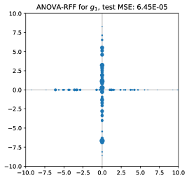
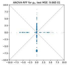
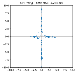
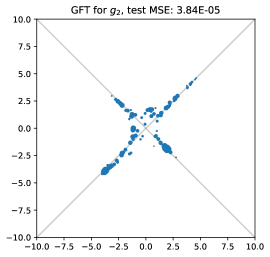
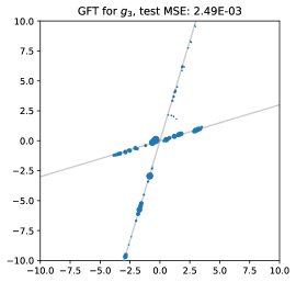
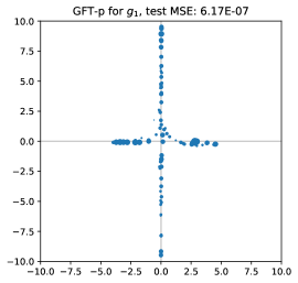
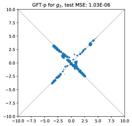
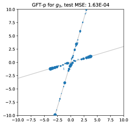
First, we inspect the learned features in a simple setting. To this end, we consider the function with . Since each summand of depends either on or , its Fourier transform is supported on the coordinate axes. To make the task more challenging, we slightly adapt the problem by also concatenating with two linear transforms , which leads to the three test functions
| (14) |
In all cases, the Fourier transform is supported on a union of two subspaces. Now, we learn the features with our GFT and GFT-p method based on samples that are drawn uniformly from , and plot the obtained locations in Figure 1. The gray lines indicate the support of the Fourier transforms of the , and the size of the markers indicates the magnitude of the associated . For all functions , the selected features are indeed located in the support of the Fourier transform. In contrast, if we do the same for methods that enforce sparse feature vectors, such as the ANOVA-RFF, the features are forced to be located on the axes. Consequently, these methods are not expected to work for and and indeed the obtained error is large. For functions where the subspaces are orthogonal, such as , this issue was recently addressed in Ba et al. (2024) by learning the associated transform in the feature space.

4.3 Function Approximation
We use the same experimental setup as in (Potts & Weidensager, 2024, Table 7.1), that is, the test functions
-
•
Polynomial: ;
-
•
Isigami: ;
-
•
Friedmann-1: .
The input dimension is set to or for each . In particular, the might not depend on all entries of the input . For their approximation, we are given samples , , and the corresponding noise-less function values . The number of samples and the input dimension are specified for each setting. As test set we draw additional samples from . We deploy our training methods GFT and GFT-p as well as standard neural network training to the architecture . The MSE on the test set are given in Table 1. There, we also include ANOVA-random Fourier features, SHRIMP and HARFE for comparison. Note that we always report the MSE for the best choice of from Potts & Weidensager, 2024, Table 7.1. We observe that GFT-p with Fourier activation functions outperforms the other approaches significantly. In particular, both the GFT and GFT-p consistently improve over the gradient-based training of the same approximation architecture . This is in line with the analysis of gradient-based training in recent works (Boob et al., 2022; Holzmüller & Steinwart, 2022). As expected, Fourier activation functions are best suited for this task.
| Method | Function | Function | Function | |||||||
| Method | Activation | |||||||||
| ANOVA-RFF | Fourier | |||||||||
| SHRIMP | Fourier | |||||||||
| HARFE | Fourier | |||||||||
| neural net | Fourier | |||||||||
| () | () | () | () | () | () | |||||
| sigmoid | ||||||||||
| () | () | () | () | () | () | |||||
| ReLU | ||||||||||
| () | () | () | () | () | () | |||||
| GFT | Fourier | |||||||||
| () | () | () | () | ( | () | |||||
| sigmoid | ||||||||||
| () | () | () | () | () | () | |||||
| GFT-p | Fourier | |||||||||
| () | () | () | () | () | () | |||||
| sigmoid | ||||||||||
| () | () | () | () | () | () | |||||
So far, we considered functions that can be represented as sums, where each summand only depends on a small number of input variables . While this assumption is crucial for the sparse Fourier feature methods from Table 1, it is not required for GFT and GFT-p. Therefore, we also benchmark our methods on the following non-decomposable functions and compare the results with standard neural network training:
-
•
-
•
, where is the vector with all entries equal to one
-
•
.
The results are given in Table 2. As in the previous case, we can see a clear advantage of GFT and GFT-p.
| Method | Function | Function | Function | ||||
|---|---|---|---|---|---|---|---|
| Method | Activation | ||||||
| neural net | Fourier | ||||||
| () | () | () | |||||
| sigmoid | |||||||
| () | () | () | |||||
| ReLU | |||||||
| () | () | () | |||||
| GFT | Fourier | ||||||
| () | () | () | |||||
| sigmoid | |||||||
| () | () | () | |||||
| GFT-p | Fourier | ||||||
| () | () | () | |||||
| sigmoid | |||||||
| () | () | () | |||||
4.4 Regression on UCI Datasets
Next, we apply our method for regression on several UCI datasets. For this setting, we do not have an underlying ground truth function . Here, we want to compare standard neural network training and our methods GFT and GFT-p with SHRIMP and SALSA. Hence, we use their numerical setup. For each method and each dataset, the MSE on the test split of the respective dataset is given in Table 3. Compared to the remaining methods, SHRIMP and SALSA appear to be a bit more robust to noise and outliers, which frequently appear in the UCI datasets. This is behavior not surprising, since the enforced sparsity of the feature vectors for those methods is a strong implicit regularization. Incorporating similar sparsity constraints on the into our generative training is left for future research. Even without such a regularization, GFT-p manages to achieve the best performance on most datasets. Again, both GFT and GFT-p achieve significantly better results than the training with the Adam optimizer.
| Method | Dataset | |||||||
| Method | Activation | Propulsion | Galaxy | Airfoil | CCPP | Telemonit | Skillkraft | |
| SHRIMP | Fourier | |||||||
| SALSA | Fourier | |||||||
| neural net | Fourier | |||||||
| () | () | () | () | () | () | |||
| sigmoid | ||||||||
| () | () | () | () | () | () | |||
| ReLU | ||||||||
| () | () | () | () | () | () | |||
| GFT | Fourier | |||||||
| () | () | () | () | () | () | |||
| sigmoid | ||||||||
| () | () | () | () | () | () | |||
| GFT-p | Fourier | |||||||
| () | () | () | () | () | () | |||
| sigmoid | ||||||||
| () | () | () | () | () | () | |||
5 Discussion
Summary
We proposed a training procedure for 2-layer neural networks with a small number of hidden neurons. In our procedure, we sample the hidden weights from a generative model and compute the optimal output weights by solving a linear system. To enhance the results, we apply a post-processing scheme in the latent space of the generative model and regularize the loss function. Numerical examples have shown that the proposed generative feature training outperforms the standard training procedure significantly.
Outlook
Our approach can be extended in several directions. First, we could train deeper networks in a greedy way similar to (Belilovsky et al., 2019). Recently, this has been also done in the context of sampled networks in (Bolager et al., 2023). Moreover, we can encode a sparse structure on the features by replacing the latent distribution with a lower-dimensional latent model or by considering mixtures of generative models. From a theoretical side, we want to characterize the global minimizers of the functional in (8) and their relations to the Fourier transform of the target function.
Limitations
If the number of hidden neurons gets large, then solving the linear system (6) becomes very expensive. However, this corresponds to the overparameterized regime where gradient-based methods should start to work again. Moreover, we computation of the optimal output layer requires to consider all data points at once, such that we cannot use minibatching. While this might slow down the training for large datasets, we would like to emphasize that 2-layer neural networks usually explicitly target the setting of small datasets, where this issue is less important.
Acknowledgments
We would like to thank Daniel Potts, Gabriele Steidl and Laura Weidensager for fruitful discussions. JH acknwoledges funding within the EPSRC programme grant “The Mathematics of Deep Learning” with reference EP/V026259/1.
References
- Acar & Vogel (1994) Robert Acar and Curtis R Vogel. Analysis of bounded variation penalty methods for ill-posed problems. Inverse Problems, 10(6):1217–1229, 1994.
- Ambrosio et al. (2000) Luigi Ambrosio, Nicola Fusco, and Diego Pallara. Functions of Bounded Variation and Free Discontinuity Problems. Oxford Mathematical Monographs. Oxford University Press, New York, 2000.
- Ba et al. (2024) Fatima Antarou Ba, Oleh Melnyk, Christian Wald, and Gabriele Steidl. Sparse additive function decompositions facing basis transforms. Foundations of Data Science, 6(4):514–552, 2024.
- Bai et al. (2023) Yatong Bai, Tanmay Gautam, and Somayeh Sojoudi. Efficient global optimization of two-layer ReLU networks: Quadratic-time algorithms and adversarial training. SIAM Journal on Mathematics of Data Science, 5(2):446–474, 2023.
- Bai et al. (2024) Yaxuan Bai, Xiaofan Lu, and Linan Zhang. Function approximations via - optimization. Journal of Applied & Numerical Optimization, 6(3):371–389, 2024.
- Barbu (2023) Adrian Barbu. Training a two-layer ReLU network analytically. Sensors, 23(8):4072, 2023.
- Belilovsky et al. (2019) Eugene Belilovsky, Michael Eickenberg, and Edouard Oyallon. Greedy layerwise learning can scale to Imagenet. In International Conference on Machine Learning, pp. 583–593. PMLR, 2019.
- Blundell et al. (2015) Charles Blundell, Julien Cornebise, Koray Kavukcuoglu, and Daan Wierstra. Weight uncertainty in neural network. In International conference on machine learning, pp. 1613–1622. PMLR, 2015.
- Bolager et al. (2023) Erik Lien Bolager, Iryna Burak, Chinmay Datar, Qing Sun, and Felix Dietrich. Sampling weights of deep neural networks. In Advances in Neural Information Processing Systems, volume 37, 2023.
- Boob et al. (2022) Digvijay Boob, Santanu S Dey, and Guanghui Lan. Complexity of training ReLU neural network. Discrete Optimization, 44:100620, 2022.
- Chan & Esedoglu (2005) Tony F Chan and Selim Esedoglu. Aspects of total variation regularized function approximation. SIAM Journal on Applied Mathematics, 65(5):1817–1837, 2005.
- Cortes et al. (2010) Corinna Cortes, Mehryar Mohri, and Ameet Talwalkar. On the impact of kernel approximation on learning accuracy. In Proceedings of the 13th International Conference on Artificial Intelligence and Statistics, pp. 113–120. JMLR, 2010.
- Dutt & Rokhlin (1993) Alok Dutt and Vladimir Rokhlin. Fast Fourier transforms for nonequispaced data. SIAM Journal on Scientific computing, 14(6):1368–1393, 1993.
- E et al. (2019) Weinan E, Chao Ma, and Lei Wu. A priori estimates of the population risk for two-layer neural networks. Communications in Mathematical Sciences, 17(5):1407–1425, 2019.
- Graves (2011) Alex Graves. Practical variational inference for neural networks. In Advances in Neural Information Processing Systems, volume 24, 2011.
- Hashemi et al. (2023) Abolfazl Hashemi, Hayden Schaeffer, Robert Shi, Ufuk Topcu, Giang Tran, and Rachel Ward. Generalization bounds for sparse random feature expansions. Applied and Computational Harmonic Analysis, 62:310–330, 2023.
- Hertrich (2024) Johannes Hertrich. Fast kernel summation in high dimensions via slicing and Fourier transforms. arXiv preprint arXiv:2401.08260, 2024.
- Hertrich et al. (2024) Johannes Hertrich, Tim Jahn, and Michael Quellmalz. Fast summation of radial kernels via QMC slicing. arXiv preprint arXiv:2410.01316, 2024.
- Holzmüller & Steinwart (2022) David Holzmüller and Ingo Steinwart. Training two-layer ReLU networks with gradient descent is inconsistent. Journal of Machine Learning Research, 23(181):1–82, 2022.
- Jospin et al. (2022) Laurent Valentin Jospin, Hamid Laga, Farid Boussaid, Wray Buntine, and Mohammed Bennamoun. Hands-on Bayesian neural networks—a tutorial for deep learning users. IEEE Computational Intelligence Magazine, 17(2):29–48, 2022. doi: 10.1109/MCI.2022.3155327.
- Kammonen et al. (2020) Aku Kammonen, Jonas Kiessling, Petr Plecháč, Mattias Sandberg, and Anders Szepessy. Adaptive random Fourier features with Metropolis sampling. arXiv preprint 2007.10683, 2020.
- Kandasamy & Yu (2016) Kirthevasan Kandasamy and Yaoliang Yu. Additive approximations in high dimensional nonparametric regression via the SALSA. In International Conference on Machine Learning, pp. 69–78. PMLR, 2016.
- Li et al. (2022) Lingfeng Li, Xue-Cheng Tai, and Jiang Yang. Generalization error analysis of neural networks with gradient based regularization. Communications in Computational Physics, 32(4):1007–1038, 2022.
- Li et al. (2021) Yang Li, Si Si, Gang Li, Cho-Jui Hsieh, and Samy Bengio. Learnable Fourier features for multi-dimensional spatial positional encoding. Advances in Neural Information Processing Systems, 34:15816–15829, 2021.
- Li et al. (2019a) Yanjun Li, Kai Zhang, Jun Wang, and Sanjiv Kumar. Learning adaptive random features. In Proceedings of the AAAI Conference on Artificial Intelligence, volume 33, pp. 4229–4236, 2019a.
- Li et al. (2019b) Zhu Li, Jean-Francois Ton, Dino Oglic, and Dino Sejdinovic. Towards a unified analysis of random Fourier features. In International Conference on Machine Learning, pp. 3905–3914. PMLR, 2019b.
- Liu et al. (2021) Fanghui Liu, Xiaolin Huang, Yudong Chen, and Johan AK Suykens. Random features for kernel approximation: A survey on algorithms, theory, and beyond. IEEE Transactions on Pattern Analysis and Machine Intelligence, 44(10):7128–7148, 2021.
- Mishkin et al. (2022) Aaron Mishkin, Arda Sahiner, and Mert Pilanci. Fast convex optimization for two-layer ReLU networks: Equivalent model classes and cone decompositions. In International Conference on Machine Learning, pp. 15770–15816. PMLR, 2022.
- Neal (2012) Radford M Neal. Bayesian Learning for Neural Networks. Springer Science & Business Media, 2012.
- Pilanci & Ergen (2020) Mert Pilanci and Tolga Ergen. Neural networks are convex regularizers: Exact polynomial-time convex optimization formulations for two-layer networks. In International Conference on Machine Learning, pp. 7695–7705. PMLR, 2020.
- Potts & Schmischke (2021) Daniel Potts and Michael Schmischke. Interpretable approximation of high-dimensional data. SIAM Journal on Mathematics of Data Science, 3(4):1301–1323, 2021.
- Potts & Weidensager (2024) Daniel Potts and Laura Weidensager. ANOVA-boosting for random Fourier features. arXiv preprint 2404.03050, 2024.
- Potts et al. (2001) Daniel Potts, Gabriele Steidl, and Manfred Tasche. Fast Fourier transforms for nonequispaced data: A tutorial. Modern Sampling Theory: Mathematics and Applications, pp. 247–270, 2001.
- Rahimi & Recht (2007) Ali Rahimi and Benjamin Recht. Random features for large-scale kernel machines. In Advances in Neural Information Processing Systems, volume 20, 2007.
- Rahimi & Recht (2008) Ali Rahimi and Benjamin Recht. Uniform approximation of functions with random bases. In 46th Annual Allerton Conference on Communication, Control, and Computing, pp. 555–561. IEEE, 2008.
- Rudi & Rosasco (2017) Alessandro Rudi and Lorenzo Rosasco. Generalization properties of learning with random features. In Advances in Neural Information Processing Systems, volume 30, 2017.
- Rux et al. (2024) Nicolaj Rux, Michael Quellmalz, and Gabriele Steidl. Slicing of radial functions: a dimension walk in the Fourier space. arXiv preprint arXiv:2408.11612, 2024.
- Saha et al. (2023) Esha Saha, Hayden Schaeffer, and Giang Tran. HARFE: Hard-ridge random feature expansion. Sampling Theory, Signal Processing, and Data Analysis, 21(2):27, 2023.
- Xie et al. (2022) Yuege Xie, Robert Shi, Hayden Schaeffer, and Rachel Ward. SHRIMP: Sparser random feature models via iterative magnitude pruning. In Bin Dong, Qianxiao Li, Lei Wang, and Zhi-Qin John Xu (eds.), Proceedings of Mathematical and Scientific Machine Learning, volume 190 of Proceedings of Machine Learning Research, pp. 303–318. PMLR, 2022.
- Yen et al. (2014) Ian En-Hsu Yen, Ting-Wei Lin, Shou-De Lin, Pradeep K Ravikumar, and Inderjit S Dhillon. Sparse random feature algorithm as coordinate descent in Hilbert space. In Advances in Neural Information Processing Systems, volume 27, 2014.