A stable multiplicative dynamical low-rank discretization for the linear Boltzmann-BGK equation
Abstract
The numerical method of dynamical low-rank approximation (DLRA) has recently been applied to various kinetic equations showing a significant reduction of the computational effort. In this paper, we apply this concept to the linear Boltzmann-Bhatnagar-Gross-Krook (Boltzmann-BGK) equation which due its high dimensionality is challenging to solve. Inspired by the special structure of the non-linear Boltzmann-BGK problem, we consider a multiplicative splitting of the distribution function. We propose a rank-adaptive DLRA scheme making use of the basis update & Galerkin integrator and combine it with an additional basis augmentation to ensure numerical stability, for which an analytical proof is given and a classical hyperbolic Courant–Friedrichs–Lewy (CFL) condition is derived. This allows for a further acceleration of computational times and a better understanding of the underlying problem in finding a suitable discretization of the system. Numerical results of a series of different test examples confirm the accuracy and efficiency of the proposed method compared to the numerical solution of the full system.
keywords:
linear Boltzmann equation, BGK relaxation model, dynamical low-rank approximation, multiplicative splitting, numerical stability, rank adaptivity1 Introduction
Numerically solving kinetic equations usually requires immense computational and memory efforts due to the high-dimensional phase space containing all possible states of the system. The state of a kinetic system is described by a distribution function which can be interpreted as the corresponding particle density in phase space. Instead of solving one high-dimensional equation, the concept of dynamical low-rank approximation (DLRA) [23] allows us to split the problem into three lower dimensional subequations leading to an appropriate approximation of the solution. In particular, in a one-dimensional setting we approximate the distribution function , with denoting the time, the spatial, and the velocity variable, by
and evolve the corresponding low-rank factors in three substeps further in time. The sets and contain the orthonormal basis functions in space and in velocity, respectively, and is called the rank of this approximation. DLRA has recently gained increasing interest and has been studied in various fields including radiation transport [2, 30, 13, 31, 34], radiation therapy [27], plasma physics [16, 18, 15, 19], chemical kinetics [32, 17] and Boltzmann type transport problems [12, 14, 11, 22]. The core idea of this method is to project the solution to a manifold of low-rank functions of the above form and constrain the solution dynamics there. Different time integrators which are able to ensure this behaviour and are robust to the presence of small singular values are available. Frequently used integrators for kinetic problems are the projector-splitting [29] as well as the (rank-adaptive) basis update & Galerkin (BUG) [10, 8] and the parallel integrator [9]. For the rank-adaptive BUG and the parallel integrator extensions to schemes with proven second-order robust error bounds have been derived in [7, 25].
For a large number of collisions, the solution of the Boltzmann-BGK equation stays close to the Maxwellian equilibrium distribution which in general is not a low-rank function. Inspired by [14, 24], we use the multiplicative splitting , for which in [14] it has been shown that is a low-rank function even if this if not the case for . Hence, we derive an evolution equation for and apply the low-rank approach to this part of the distribution function. Difficulties may arise in the discretization as it is per se not clear how to treat spatial derivatives.
In this paper we propose a stable dynamical low-rank discretization for the linear Boltzmann-BGK equation. The main features of this paper are:
-
1.
A multiplicative splitting of the distribution function: As the Maxwellian equilibrium distribution is generally not a low-rank function, we consider the multiplicative splitting and apply the low-rank ansatz to the remaining function . It can be considered as a deviation from the equilibrium and is shown to be of low rank [14].
-
2.
A stable numerical scheme for linear Boltzmann-BGK with rigorous mathematical proofs: We show that a stable discretization has to be derived carefully and compare it with an intuitive discretization that fails to guarantee numerical stability. We give a rigorous analytical proof of stability and derive a classic hyperbolic CFL condition. This enables us to choose an optimal time step size of with CFL denoting the CFL number, leading to a reduction of the computational effort.
-
3.
A rank-adaptive integrator: For the low-rank scheme we use the rank-adaptive BUG integrator from [8], leading to a basis augmentation in both the - and -step of the low-rank algorithm. Compared to the projector-splitting integrator used in [12, 14, 11], this allows us to determine the rank adaptively in each step avoiding the a priori choice of a certain fixed rank.
-
4.
A series of numerical experiments validating the derived properties: We give a number of numerical examples that validate the derived stability while showing a significant reduction of computational and memory requirements of the low-rank scheme compared to the full order method.
The paper is structured as follows: After the introduction in Section 1, we provide background information on the linear Boltzmann-BGK equation, explain the considered multiplicative structure, and derive two possible systems of equations in Section 2. Both systems are equivalent in the continuous setting. In Section 3, we discretize in velocity and in space, before subsequently time is discretized giving two different fully discretized schemes. It is then shown in Section 4 that a naive discretization can lead to a numerical scheme that is not von Neumann stable whereas a more careful treatment guarantees numerical stability. Section 5 gives a brief introduction to the concept of DLRA and applies this method such that a numerically stable low-rank scheme is obtained. Numerical experiments in both D and D in Section 6 confirm the derived results. Section 7 gives a brief conclusion and outlook.
2 Linear Boltzmann-BGK
The Boltzmann equation is a fundamental model in kinetic theory describing a gas that is not in thermodynamic equilibrium [6, 33]. In its full formulation it makes use of the so called “Stosszahlansatz” leading to a collision operator for which the solution of the Boltzmann equation is demanding. To overcome this, the BGK model [4], named after Bhatnagar, Gross and Krook, can be considered. It simplifies the collision term while maintaining the key properties of the equation. In a one-dimensional setting it reads
| (1a) | ||||
| where denotes the distribution function depending on the time , the spatial variable and the velocity variable . The constant describes the collisionality of the particles and stands for the Maxwellian equilibrium distribution. It depends on the density for which we obtain an evolution equation by integrating (1a) with respect to . This gives | ||||
| (1b) | ||||
In [14] it has been shown that using the multiplicative decomposition
| (2) |
is advantageous as is low-rank even if this is not the case for the Maxwellian (which is not true for the classic additive micro-macro decomposition). In order to reduce computational and memory costs a dynamical low-rank approach has then been applied in [14] to treat the resulting evolution equations for .
In this work, we consider an isothermal Maxwellian without drift, i.e.
This results in a linear model, which we call the linear Boltzmann-BGK equation. It has been extensively studied in the PDE community (see, e.g., [20, 5, 1]) as well as from a numerical point of view [3]. In this paper, we provide a stability analysis of this model in the context of dynamical low-rank simulation. The stability analysis for the simplified problem provides insight into the numerical schemes that have been used in the literature [14] for the Boltzmann–BGK equation. In particular, it explains why such schemes need to take relatively small time step sizes even though the collision operator is treated implicitly.
We insert the multiplicative approach (2) into (1a) and (1b) and obtain
| (3a) | ||||
| (3b) | ||||
This set of equations is called the advection form of the multiplicative system. It corresponds to the way the equations are treated in [14]. We can rewrite equation (3a) into a conservative form, leading to the system
| (4a) | ||||
| (4b) | ||||
Note that for both systems we omit initial and boundary conditions for now. It is a challenging task to construct a suitable numerical scheme as it is per se not clear how to treat the spatial derivative in the transport part of the first equations and which of both systems to prefer. Further, the potentially stiff collision term requires an implicit time discretization. In addition, the consideration of higher dimensionality occurring in practical applications leads to prohibitive numerical costs. To overcome this last problem, we make use of the numerical reduced order method of dynamical low-rank approximation after having derived a stable discretization.
3 Discretization of the system
In this section we give a full discretization of both versions (3) and (4) of the system. We start with discretizing equations (3) and (4) in velocity and space before a time discretization is presented in the next subsection.
3.1 Discretization in velocity and in space
For the discretization in the velocity space we use a nodal approach and prescribe a certain number of grid points . Due to the special structure of (3b) and (4b) we use a Gauss-Hermite quadrature providing the quadrature nodes and weights enabling us to approximate integrals as
For the discretization of the spatial domain we take grid points and choose a grid with equidistant spacing . We approximate -dependent quantities by
Spatial derivatives are approximated by the tridiagonal stencil matrices corresponding to a first-order central differencing scheme. Further, a tridiagonal second-order central differencing stabilization matrix approximating is added. Their entries are defined as
whereas all other entries are set to zero. Note that from now on we assume periodic boundary conditions. For this reason we set
Similar to the proof in [2], one can show that the stencil matrices and fulfill the following properties:
Lemma 1 (Summation by parts).
Let with indices . Then it holds
Moreover, let be defined as
Then, .
We insert the proposed velocity and space discretization into the advection form (3) and add a stabilizing second-order term for . This corresponds to the method used in [14] for the non-linear isothermal Boltzmann-BGK equation and leads to the semi-discrete time-continuous system
| (5a) | ||||
| (5b) | ||||
For the conservative form (4) the second-order stabilization term is applied to . We obtain the semi-discrete system
| (6a) | ||||
| (6b) | ||||
3.2 Time discretization
The time discretization of both systems has to be derived carefully to ensure numerical stability. We start with the advection form (5) and perform an explicit Euler step for the transport part in (5a) as well as in (5b). The potentially stiff collision term is treated implicitly. For approximating the time derivative the corresponding difference quotient is used. We obtain the fully discrete scheme
| (7a) | ||||
| (7b) | ||||
For the conservative form (6) we again perform an explicit Euler step for the transport part in (6a) as well as in (6b). The collision term is treated implicitly and a factor coming from the analysis is added. As before, the time derivative is approximated by its difference quotient. This leads to the fully discretized equations
| (8a) | ||||
| (8b) | ||||
Note that the discretizations for given in (7b) and (8b) are exactly the same. The main differences between the naive discretization of the advection form (7) and the proposed scheme (8) are the stabilization of in (8a), opposed to a stabilization of as done in (7a), and the additional factor in the collision term of (8a).
In the fully discrete setting, we make use of the following notations.
Definition 1 (Fully discrete solution and Maxwellian).
The full solution of the linear Boltzmann-BGK equation in the fully discrete setting at time is given by with entries
For the fully discrete Maxwellian at time , we have .
4 Numerical stability
Although the derivation of the equations in (7) and (8) is similar, both systems differ drastically in terms of numerical stability. In this section, both fully discretized schemes presented are compared.
4.1 Naive discretization
We begin with the naive discretization given in (7) that is comparable to the one chosen in [14] in the sense that the advection form of the multiplicative splitting is used. In [14], numerical experiments are given but no explicit stability analysis is conducted. In the following, we give an example which shows that numerical stability in the sense of von Neumann can not be guaranteed.
Theorem 1.
There exist initial values and such that the numerical scheme proposed in (7) for is not von Neumann stable.
Proof.
Let us assume a solution that is constant in space and velocity, e.g. . For this solution the terms containing and are zero. Let us further assume that there is no collisionality, i.e. . We insert this information into (7a) and get
4.2 Stable discretization
Having seen that for a certain choice of the initial values the system of equations (7) is not von Neumann stable, we now consider equations (8) in terms of numerical stability. We observe that the advection terms are treated explicitly, whereas the collision term is treated implicitly, leading to a removal of the potential stiffness caused by a large number of collisions. We seek a rigorous proof of stability under a classic hyperbolic CFL condition that will be derived in the following norm.
Definition 2 (Stability norm).
For , the -norm shall be defined as
This corresponds to a Frobenius norm with weights .
The choice of this norm is inspired by the analysis in [1], where hypocoercivity for the linear Boltzmann-BGK equation is shown. Different from there, we use a fully discrete analogue to the considered weighted -norm that also takes the Gauss-Hermite quadrature into account. Note that the factor does not affect the stability but is added for consistency in the sense that for the condition holds. This is the discrete counterpart of which is equivalent to that in a discrete formulation can be written as . This relation shall be preserved by the numerical scheme.
Lemma 2.
Let us assume that the initial condition for satisfies . Then, for all we have
Proof.
We start from equation (8a), bring the terms containing to the left-hand side and multiply it with . This gives
Multiplication with and summation over leads to
We insert the induction assumption as well as . Then, together with (8b), we get
Cancelling with gives the desired equality, and completes the proof. ∎
Also, the following inequality is indispensable to show numerical stability of the above system.
Lemma 3.
Under the time step restriction it holds
Proof.
We want to apply a Fourier analysis in that allows us to write the stencil matrices in diagonal form. As in [2, 26], we define the matrix as
where denotes the imaginary unit. It is orthonormal, i.e. , where the superscript stands for the complex transpose, and diagonalizes the stencil matrices
with being the diagonal matrices with entries
and . Let us denote with entries . With Parseval’s identity we obtain
A sufficient condition to ensure negativity is that
must hold for each index . This leads to the time step restriction , which proves the lemma. ∎
We can now show numerical stability of the proposed system.
Theorem 2.
Under the time step restriction , the fully discrete system (8) is numerically stable in the -norm, i.e.
Proof.
We multiply (8a) with and bring the last term of the equation from the right-hand to the left-hand side. This gives
Multiplication with then leads to
Note that it holds
We insert this relation and obtain
In the next step, we multiply with and sum over and . This gives
From Lemma 2 we have that . Hence, we can derive that the following term is equal to zero. Lemma 2 gives that also the term is equal to zero. We subtract both and add an additional zero by adding and subtracting the second-order term . This leads to
| (I) | ||||
| (II) | ||||
| (III) | ||||
Now, we consider the parts (I), (II) and (III) separately. Let us start with (I) and (II) and apply Young’s inequality which states that for it holds that . This gives for (I) +(II)
For (III) we get with the properties of the stencil matrices given in Lemma 1 that
Inserting these relations then gives
With Lemma 3 we can conclude that under the CFL condition it holds . Hence, with this time step the proposed fully discrete system (8) is numerically stable in the -norm. ∎
5 Dynamical low-rank approximation for the stable system
In practical applications, the implementation of the full system given in (8) may lead to prohibitive numerical costs, especially when computing in higher dimensional settings. To reduce computational and memory demands, we apply dynamical low-rank approximation to the distribution function .
5.1 Background on dynamical low-rank approximation
The concept of dynamical low-rank approximation has been introduced in a semi-discrete time-dependent matrix setting [23]. Let us consider being the solution of the matrix differential equation
where denotes the right-hand side of the equation. We then seek for an approximation of in the following form
| (10) |
with and denoting the orthonormal spatial and orthonormal velocity basis, respectively. The slim matrix is called the coefficient or coupling matrix and determines the rank of the approximation. The set of all matrices of the above form (10) constitute the low-rank manifold . Its corresponding tangent space at shall be denoted by . We now look for such that at all times the minimization problem
is fulfilled. Following [23], this minimization constraint is equivalent to determining by an orthogonal projection onto the tangent space such that
| (11) |
where the orthogonal projector onto applied to an arbitrary quantity can explicitly be given as
Different robust time integrators to solve (11) exist. Frequently used integrators are the projector-splitting integrator [29], the basis update & Galerkin integrator [10] as well as its rank-adaptive extension [8] and the parallel integrator [9]. In this paper, we make use of the rank-adaptive BUG integrator whose concept shall be explained in the following.
In the first two steps, the rank-adaptive BUG integrator updates and augments the bases and in parallel such that their rank increases from to , for the spatial and velocity basis respectively. We denote the augmented quantities of rank with hats. Then, for the augmented bases a Galerkin step is performed before in a last step a new rank is determined using a truncation with prescribed tolerance. In detail, the rank-adaptive BUG integrator performs the following steps in order to update the matrix at time to at time :
K-Step: Let us fix the velocity basis at time and introduce the notation . The spatial basis is updated and augmented by first solving the PDE
and then determining as an orthonormal basis of , e.g. by QR-decomposition. Then, we compute .
L-Step: Let us fix the spatial basis at time and introduce the notation . The velocity basis is updated and augmented by first solving the PDE
and then determining as an orthonormal basis of , e.g. by QR-decomposition. Then, we compute .
S-step: Update the coupling matrix from to by solving the ODE
Truncation: Compute the singular value decomposition of with . For a prescribed tolerance parameter the new rank is chosen such that
Let now contain the largest singular values and and contain the first columns of and , respectively. Then, the time-updated spatial basis can be determined as and the time-updated velocity basis as .
Altogether, the time-updated approximation of the distribution function after one time step is given by .
5.2 DLRA algorithm for multiplicative linear Boltzmann-BGK
In this section, we apply DLRA to the stable and fully discretized system (8). Bringing all term containing to the left-hand side of (8a) and multiplying it with , equations (8) can be equivalently written as
| (12a) | ||||
| (12b) | ||||
We propose a low-rank implementation that uses the rank-adaptive BUG integrator [8] introduced in the previous subsection for equation (12a) together with an additional basis augmentation and a suitable truncation strategy. For this scheme we show numerical stability. Note that in the following, for simplicity, we write instead of .
Starting from (12), we apply the rank-adaptive BUG integrator leading to a splitting of (12a) into three substeps, the -, -, and -step. In the - as well as in the -step we perform an additional basis augmentation ensuring certain quantities to be contained in the basis at all times. The augmented bases are then used to determine the -step. Note that the scattering term is only applied in the -step as it does not affect the span of the basis functions derived in the - and -step. We obtain the following DLRA scheme:
| Substituting into the update equation (12b) yields | ||||
| (13a) | ||||
| For the -step we introduce the notation and solve | ||||
| (13b) | ||||
| This gives the updated matrix to which together with the old basis a QR-decomposition is applied, giving the new augmented basis . | ||||
In addition, we augment this basis according to
| (13c) |
leading to a new augmented basis of rank , and we compute . Note that all quantities of rank are denoted with one hat and all quantities of rank with double hats.
For the -step we write and solve
| (13d) |
This gives the updated matrix to which together with the old basis a QR-decomposition is applied, giving the new augmented basis .
In addition, we augment this basis according to
| (13e) |
leading to a new augmented basis of rank , and we compute .
For the -step we denote and insert the expressions and into (12a). We multiply with and sum over and . This leads to
| (13f) |
The last step consists in truncating the augmented quantities , and from rank to a new rank . We use a modification of the truncation strategy described in Section 5.1 that ensures that stays valid in each time step and works as follows:
Let us denote being the vector with entries and let , where stands for the Euclidean norm. We then want to have
with , denoting the identity matrix and the vector containing ones at each entry. is a matrix of rank . We determine its low-rank factors by a singular value decomposition such that with , and . For , it holds that . We apply the truncation strategy from Section 5.1 to and obtain and , which shall be of rank . Finally, we combine both parts by performing a QR-decomposition of
and setting
The new rank is then given by . With the time-updated low-rank factors , and , the updated low-rank approximation of the solution is . The steps of the proposed DLRA scheme are visualized in Figure 1.
From the low-rank approximation of we can regain the full solution as follows.
Definition 3 (Low-rank approximation of the full solution).
The DLRA approximation of the full solution of the linear Boltzmann-BGK equation in the fully discrete setting at time is given by with entries
5.3 Stability of the proposed low-rank scheme
We can then show that algorithm (5.2) is numerically stable.
Theorem 3.
Under the time step restriction , the fully discrete DLRA scheme (5.2) is numerically stable in the -norm, i.e
Proof.
We start from the -step in (13f), multiply it with and and sum over and . For simplicity of notation, we introduce the projections and . This gives
Multiplication with and summation over and leads to
We now use the fact that we have augmented the bases in (13c) and (13e) such that
holds. We insert these relations and, to be consistent in notation, change the summation indices on the left-hand side from to and to giving
Analogously to the proof of Theorem 2 and, as the truncation step is designed not to alter these expressions, we can conclude that the proposed DLRA scheme is numerically stable under the time step restriction . ∎
6 Numerical results
To validate the theoretical considerations and the proposed DLRA scheme, numerical results for different test examples in 1D as well as in 2D are given in this section.
6.1 1D Plane source
We start with a one-dimensional analogue to the plane source problem, which is a common test case for radiative transfer [2, 8, 26, 31], and compare the solution of the full equations (8) to the solution obtained by the DLRA scheme given in (5.2). The spatial domain shall be set to . As initial conditions we choose the density to be a cutoff Gaussian
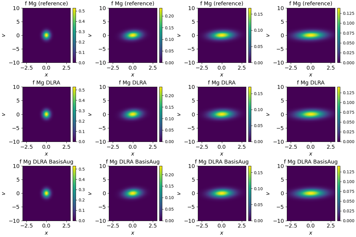
where denotes a constant deviation, and the function to be constant in space and velocity, i.e. . We consider relatively large collisionality by choosing . Computations are started with an initial rank of . As computational parameters we use grid points in the spatial as well as grid points in the velocity domain. Due to this choice, we obtain , which shall be adjusted to the next larger integer value such that the time step size is determined by with , according to the corresponding CFL condition. Practical implementations now show that the basis augmentations to rank in in (13c) and (13e) needed for the theoretical proof of the numerical stability may not be necessary for numerical examples and that the standard basis augmentations to rank provide similar solutions while being significantly faster. For this reason, we propose to leave out the basis augmentations (13c) and (13e) in practical applications. In this case, all quantities with double hats related to rank reduce to quantities of rank with one single hat. The simplified scheme with rank is also visualized (in brackets) in the flowchart of Figure 1. In Figure 2, we now compare the results for the full solution , computed with the full solver (Mg (reference)), the DLRA scheme with rank (Mg DLRA) and the basis augmented DLRA scheme with rank (Mg DLRA BasisAug) at different times up to . We observe that the reduced as well as the augmented DLRA algorithm capture the main characteristics of the full reference Mg system.
This is also true for the computational results for the density , displayed in Figure 3.
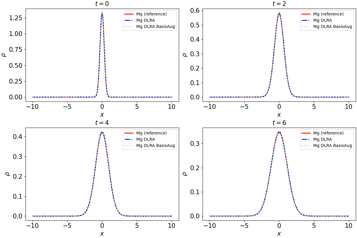
Figure 4 shows the evolution of the rank, which for a chosen tolerance parameter of increases up to before it significantly reduces over time. Note that the evolution of the rank for the reduced as well as for the basis augmented algorithm show good agreement as the new rank is displayed after the corresponding truncation step. Further, the behavior of the norm is depicted. As expected, it decreases smoothly over time for all considered systems. Additionally, we display the quantities and . It is essential that they are equal to , which for the low-rank schemes is ensured by the adjusted truncation step. It can be observed that this property is fulfilled up to order .
6.2 2D Plane source
In higher dimensions, the computational advantages of DLRA schemes are enhanced. For this reason, we give some two-dimensional test examples starting with the two-dimensional version of the plane source problem considered in the previous section. The corresponding two-dimensional set of equations becomes
where and . We compare the solution of this system with the solution of the DLRA scheme for which the extension to the two-dimensional setting is straightforward. For this test example we choose the spatial domain and prescribe the initial condition for the density by
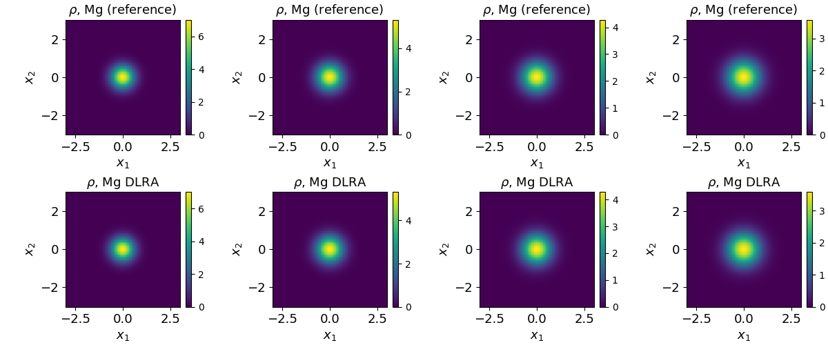
with a constant deviation of . The function shall be set to and the collision coefficient to . We allow an initial rank of . Computations are performed on a spatial grid with grid points in and grid points in . For the velocity grid we choose grid points in and grid points in . Due to this choice, we obtain which shall be adjusted to the next larger integer value such that the time step size is determined by with a CFL number of . Figure 5 compares the density at different times up to , computed with the full solver (Mg (reference)) and the reduced DLRA scheme with rank (Mg DLRA). Note that we refrain from computations with the basis augmented scheme as in two space and velocity dimensions this would lead to extremely increased computational costs. We observe that the solution of the DLRA scheme matches the solution of the full system.
To determine the evolution of the rank, we use a tolerance parameter of . In Figure 6, we observe an increasing up to before it decreases continuously over time. Further, the norm is displayed. It decreases smoothly over time for all considered systems. In addition, we plot the quantities and , which are equal to up to order .
For this setup, the running time of the DLRA scheme compared to the full solver is clearly faster. It reduces by a factor of approximately 2 from 3954 seconds to 1926 seconds, confirming the computational advantages of the DLRA scheme.
6.3 2D Beam
As a second two-dimensional test example we consider a beam in the spatial domain starting at in the middle of the spatial plane and moving to the bottom left. The initial values are given by
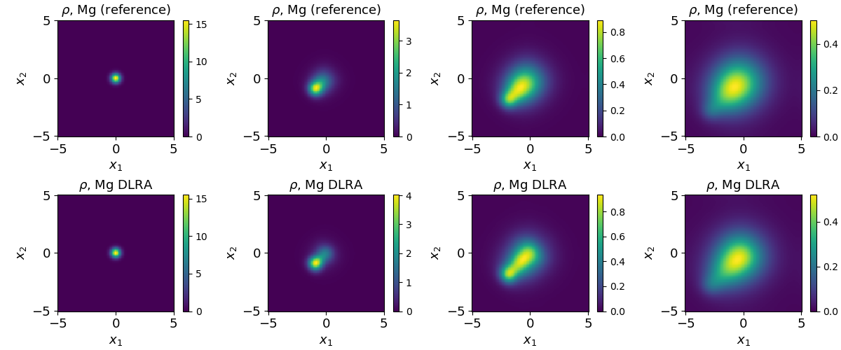
where and is a normalization constant such that holds. The beam velocity is set to and the collisionality to . The initial rank is given as . Computations are performed on a spatial grid with grid points in and grid points in . For the velocity grid we choose grid points in and grid points in . As before, this leads to a time step size of with a CFL number of . Figure 7 compares the density at different times up to , computed with the full solver (Mg (reference)) and the reduced DLRA scheme with rank (Mg DLRA). At all displayed time steps the DLRA solution resembles the solution of the full system.
In Figure 8, the evolution of the rank in time is shown. We use a tolerance parameter of and allow a maximal rank of . Due to the choice of the solution of the problem is not low-rank. For this reason, we observe an increasing of the rank up to the maximal allowed value. Also, the norm is depicted over time. It decreases continuously, matching our theoretical considerations. Further, it can be observed that the quantities and are equal to up to order .
Due to the high rank, the running time of the DLRA scheme compared with the full solver is slightly increased. This example illustrates the relation between the choice of and the low-rank structure of the solution. It is expected that for larger values of the solution becomes low-rank and hence the computational benefits of the DLRA scheme are enhanced.
7 Conclusion and outlook
We have derived a multiplicative DLRA discretization for the linear Boltzmann-BGK problem that in contrast to another presented naive discretization is numerically stable. To show this, we have conducted a stability analysis leading to a concrete hyperbolic CFL condition. In addition, numerical examples in 1D and 2D confirm the stability, accuracy and efficiency of the proposed DLRA scheme.
The insights gained from this article can be helpful for future work as the employed multiplicative splitting is attached to the investigation of more complicated equations, e.g. the non-linear Boltzmann-BGK equation treated in [14]. However, a direct transition of knowledge is hardly possible as for the non-linear case most of the theoretical concepts applied here are not available, making the analysis much more difficult to consider. Further, in the non-linear case a discretization of the conservative form of the equations, i.e. by not splitting up the term , is possible but cannot be efficiently implemented as the Maxwellian is generally not low-rank. Even though, we propose to reconsider the chosen discretization in [14] in terms of stabilization, which may allow for a larger time step size leading to an even more efficient DLRA algorithm.
Acknowledgements
The authors thank Marlies Pirner for helpful discussions on the linear Boltzmann-BGK equation. Lena Baumann acknowledges support by the Würzburg Mathematics Center for Communication and Interaction (WMCCI) as well as the Stiftung der Deutschen Wirtschaft.
References
- [1] F. Achleitner, A. Arnold, and E. A. Carlen. On linear hypocoercive BGK models. In P. Gonçalves and A. J. Soares, editors, From Particle Systems to Partial Differential Equations III. Springer Proceedings in Mathematics & Statistics, volume 162, pages 1–37, Cham, 2016. Springer.
- [2] L. Baumann, L. Einkemmer, C. Klingenberg, and J. Kusch. Energy stable and conservative dynamical low-rank approximation for the Su-Olson problem. SIAM Journal on Scientific Computing, 46(2):B137–B158, 2024.
- [3] M. Bessemoulin-Chatard, M. Herda, and T. Rey. Hypocoercivity and diffusion limit of a finite volume scheme for linear kinetic equations. Mathematics of Computation, 89(323):1093–1133, 2020.
- [4] E. P. Bhatnagar, T. Gross, and M. Krook. A model for collision processes in gases. I. Small amplitude processes in charged and neutral one-component systems. Physical Review, 94(3):511–525, 1954.
- [5] J. A. Cañizo, C. Cao, J. Evans, and H. Yoldaş. Hypocoercivity of linear kinetic equations via Harris’s Theorem. Kinetic and Related Models, 13(1):97–128, 2020.
- [6] C. Cercignani. The Boltzmann Equation and Its Applications. Springer, New York, 1988.
- [7] G. Ceruti, L. Einkemmer, J. Kusch, and C. Lubich. A robust second-order low-rank BUG integrator based on the midpoint rule. arXiv preprint arXiv:2402.08607, 2024.
- [8] G. Ceruti, J. Kusch, and C. Lubich. A rank-adaptive robust integrator for dynamical low-rank approximation. BIT Numerical Mathematics, 62:1149–1174, 2022.
- [9] G. Ceruti, J. Kusch, and C. Lubich. A parallel rank-adaptive integrator for dynamical low-rank approximation. SIAM Journal on Scientific Computing, 46(3):B205–B228, 2024.
- [10] G. Ceruti and C. Lubich. An unconventional robust integrator for dynamical low-rank approximation. BIT Numerical Mathematics, 62(1):23–44, 2022.
- [11] Z. Ding, L. Einkemmer, and Q. Li. Dynamical low-rank integrator for the linear Boltzmann equation: error analysis in the diffusion limit. SIAM Journal on Numerical Analysis, 59(4):2254–2285, 2021.
- [12] L. Einkemmer. A low-rank algorithm for weakly compressible flow. SIAM Journal on Scientific Computing, 41(5):A2795–A2814, 2019.
- [13] L. Einkemmer, J. Hu, and J. Kusch. Asymptotic-preserving and energy stable dynamical low-rank approximation. SIAM Journal on Numerical Analysis, 62(1):73–92, 2024.
- [14] L. Einkemmer, J. Hu, and L. Ying. An efficient dynamical low-rank algorithm for the Boltzmann-BGK equation close to the compressible viscous flow regime. SIAM Journal on Scientific Computing, 43(5):B1057–B1080, 2021.
- [15] L. Einkemmer and I. Joseph. A mass, momentum, and energy conservative dynamical low-rank scheme for the Vlasov equation. Journal of Computational Physics, 443:110493, 2021.
- [16] L. Einkemmer and C. Lubich. A low-rank projector-splitting integrator for the Vlasov-Poisson equation. SIAM Journal on Scientific Computing, 40(5):B1330–B1360, 2018.
- [17] L. Einkemmer, J. Mangott, and M. Prugger. A low-rank complexity reduction algorithm for the high-dimensional kinetic chemical master equation. Journal of Computational Physics, 503:112827, 2024.
- [18] L. Einkemmer, A. Ostermann, and C. Piazzola. A low-rank projector-splitting integrator for the Vlasov–Maxwell equations with divergence correction. Journal of Computational Physics, 403:109063, 2020.
- [19] L. Einkemmer, A. Ostermann, and C. Scalone. A robust and conservative dynamical low-rank algorithm. Journal of Computational Physics, 484:112060, 2023.
- [20] J. Evans. Hypocoercivity in Phi-entropy for the linear relaxation Boltzmann equation on the torus. SIAM Journal on Mathematical Analysis, 53(2):1357–1378, 2021.
- [21] E. Hairer and G. Wanner. Solving Ordinary Differential Equations II: Stiff and Differential-Algebraic Problems. Springer Berlin, Heidelberg, 1996.
- [22] J. Hu and Y. Wang. An adaptive dynamical low rank method for the nonlinear Boltzmann equation. Journal of Scientific Computing, 92:75, 2022.
- [23] O. Koch and C. Lubich. Dynamical low-rank approximation. SIAM Journal on Matrix Analysis and Applications, 29(2):434–454, 2007.
- [24] K. Kormann and E. Sonnendrüecker. Sparse grids for the Vlasov–Poisson equation. In J. Garcke and D. Pflüger, editors, Sparse Grids and Applications – Stuttgart 2014. Lecture Notes in Computational Science and Engineering, volume 109, pages 163–190, Cham, 2016. Springer.
- [25] J. Kusch. Second-order robust parallel integrators for dynamical low-rank approximation. arXiv preprint arXiv:2403.02834, 2024.
- [26] J. Kusch, L. Einkemmer, and G. Ceruti. On the stability of robust dynamical low-rank approximations for hyperbolic problems. SIAM Journal on Scientific Computing, 45(1):A1–A24, 2023.
- [27] J. Kusch and P. Stammer. A robust collision source method for rank adaptive dynamical low-rank approximation in radiation therapy. ESAIM: M2AN, 57(2):865–891, 2023.
- [28] R. J. LeVeque. Finite Volume Methods for Hyperbolic Problems. Cambridge University Press, Cambridge, 2002.
- [29] C. Lubich and I. V. Oseledets. A projector-splitting integrator for dynamical low-rank approximation. BIT Numerical Mathematics, 54(1):171–188, 2014.
- [30] C. Patwardhan, M. Frank, and J. Kusch. Asymptotic-preserving and energy stable dynamical low-rank approximation for thermal radiative transfer equations. arXiv preprint arXiv:2402.16746, 2024.
- [31] Z. Peng, R. G. McClarren, and M. Frank. A low-rank method for two-dimensional time-dependent radiation transport calculations. Journal of Computational Physics, 421:109735, 2020.
- [32] M. Prugger, L. Einkemmer, and C. F. Lopez. A dynamical low-rank approach to solve the chemical master equation for biological reaction networks. Journal of Computational Physics, 489:112250, 2023.
- [33] H. Struchtrup. Macroscopic Transport Equations for Rarefied Gas Flows. Approximation Methods in Kinetic Theory. Springer, Berlin, Heidelberg, 2005.
- [34] P. Yin, E. Endeve, C. D. Hauck, and S. R. Schnake. A semi-implicit dynamical low-rank discontinuous Galerkin method for space homogeneous kinetic equations. Part I: emission and absorption. arXiv preprint arXiv:2308.05914, 2023.