Particle creation and evaporation in Kalb–Ramond gravity

Abstract

In this work, we examine particle creation and the evaporation process in the context of Kalb–Ramond gravity. Specifically, we build upon two existing solutions from the literature yang2023static and Liu:2024oas , both addressing a static, spherically symmetric configuration. For this study, we focus on the scenario in which the cosmological constant vanishes. To begin, the corrections to Hawking radiation for bosonic modes are examined by studying the Klein–Gordon equation in curved spacetime. Through the calculation of Bogoliubov coefficients, we identify how the parameter $\ell$, which governs Lorentz symmetry breaking, contributes a correction to the amplitude associated with particle production. Within this approach, the power spectrum and Hawking temperature are derived. Additionally, we obtain expressions for the power spectrum and particle number density by analyzing Hawking radiation from a tunneling viewpoint. A parallel approach is applied to fermionic modes. Finally, we examine black hole evaporation, finding that the black hole lifetime in these cases can be determined analytically.

I Introduction

A fundamental principle in modern physics, Lorentz symmetry holds that physical laws apply consistently across all inertial frames. This symmetry is extensively validated through experimental and observational evidence; however, certain high–energy scenarios in theoretical physics propose that it may not be absolute. Various frameworks — such as loop quantum gravity 2 , string theory 1 , non–commutative field theory 4 ; araujo2023thermodynamics ; heidari2023gravitational , Hořava–Lifshitz gravity 3 , massive gravity 6 , Einstein–aether theory 5 , very special relativity 8 , and $f(T)$ gravity 7 — explore conditions under which Lorentz invariance is no longer maintained.

Two main types of Lorentz symmetry breaking (LSB) are recognized: explicit and spontaneous bluhm2006overview . In the case of explicit breaking, Lorentz invariance is absent in the Lagrangian density itself, causing physical laws to differ across specific reference frames. On the other hand, spontaneous symmetry breaking occurs when the Lagrangian density remains Lorentz–invariant, yet the system’s ground state does not uphold this symmetry bluhm2008spontaneous .

Research on spontaneous Lorentz symmetry breaking 12 ; KhodadiPoDU2023 ; AraujoFilho:2024ykw ; 13 ; 11 ; 9 ; 10 ; filho2023vacuum is grounded in the framework of the Standard Model Extension, where the simplest theoretical approaches are represented by bumblebee models KhodadiEPJC2023 ; 12 ; 10 ; 1 ; 11 ; 13 ; KhodadiEPJC20232 ; CapozzielloJCAP2023 ; KhodadiPRD2022 . In these models, a vector field known as the bumblebee field acquires a non–zero vacuum expectation value (VEV), establishing a preferred spatial direction and thus breaking local Lorentz invariance for particles. This symmetry breaking has significant implications, especially for thermodynamic properties aa2021lorentz ; paperrainbow ; aa2022particles ; araujo2021higher ; araujo2021thermodynamic ; araujo2022does ; aaa2021thermodynamics ; anacleto2018lorentz ; petrov2021bouncing2 ; reis2021thermal ; araujo2022thermal .

An exact solution for a static, spherically symmetric spacetime within bumblebee gravity is introduced in Ref. 14 . In a comparable manner, a Schwarzschild–like solution has been extensively analyzed from several angles, including studies on gravitational lensing 15 , accretion dynamics 18 ; 17 , quasinormal modes 19 , and Hawking radiation 16 .

Building upon earlier work, Maluf et al. derived an (A)dS–Schwarzschild–like solution that does not require strict vacuum conditions 20 . In a similar manner, Xu et al. introduced additional types of static, spherically symmetric bumblebee black holes by incorporating a background bumblebee field with a non–zero time component. This allowed them to investigate the thermodynamic properties and observational signatures of these solutions, as outlined in Refs. 24 ; 23 ; 22 ; 21 .

An alternative framework for studying LSB involves the rank–two antisymmetric tensor field, known as the Kalb–Ramond field 42 ; maluf2019antisymmetric , which naturally emerges in bosonic string theory 43 . When this field is coupled to gravity in a non–minimal way and develops a non–zero VEV, it induces spontaneous Lorentz symmetry breaking. In 44 , a solution is provided for a static, spherically symmetric configuration within this context. Subsequent research examined the motion of massive and massless particles near this static spherical Kalb–Ramond black hole 45 . Additionally, 46 investigates gravitational lensing and shadow patterns produced by rotating black holes influenced by the Kalb–Ramond field.

In addition, Ref. yang2023static presents a set of new exact solutions for static and spherically symmetric spacetimes, developed both with and without a cosmological constant. These ones are constructed within a framework where the Kalb–Ramond field has a non–zero vacuum expectation value. Later, Ref. Liu:2024oas reveals an alternative black hole configuration that had not been previously explored in yang2023static .

Furthermore, Hawking’s work established a crucial connection between quantum mechanics and gravity, laying the groundwork for quantum gravity theory o1 ; o11 ; o111 . His research revealed that black holes can emit thermal radiation and slowly diminish over time, a phenomenon known as Hawking radiation eeeOvgun:2019ygw ; gibbons1977cosmological ; eeeKuang:2017sqa ; eeeKuang:2018goo ; eeeOvgun:2019jdo ; eeeOvgun:2015box . This result, derived from quantum field theory near a black hole’s event horizon, has significantly advanced the study of black hole thermodynamics and quantum processes in strong gravitational fields sedaghatnia2023thermodynamical ; o9 ; o6 ; araujo2024dark ; o4 ; o3 ; o7 ; aa2024implications ; araujo2023analysis ; o8 . Later, Kraus and Wilczek o10 , followed by Parikh and Wilczek o13 ; o12 ; 011 , interpreted Hawking radiation as a tunneling effect within a semi–classical framework. This approach has since been widely applied across various black hole models, offering important perspectives on black hole properties johnson2020hawking ; senjaya2024bocharova ; vanzo2011tunnelling ; calmet2023quantum ; mirekhtiary2024tunneling ; anacleto2015quantum ; mitra2007hawking ; silva2013quantum ; medved2002radiation ; del2024tunneling ; zhang2005new ; touati2024quantum .

In this manner, this study investigates particle creation and black hole evaporation within the framework of Kalb–Ramond gravity. We build on two established solutions from the literature yang2023static ; Liu:2024oas , both of which describe static, spherically symmetric spacetimes, focusing specifically on cases where the cosmological constant is zero. Our analysis begins by exploring corrections to Hawking radiation for bosonic modes through the Klein–Gordon equation in curved spacetime. By calculating the Bogoliubov coefficients, we demonstrate how the Lorentz symmetry–breaking parameter $\ell$ modifies the amplitude for particle production. This approach allows us to derive expressions for both the power spectrum and the Hawking temperature. We further analyze the power spectrum and particle number density using a tunneling perspective on Hawking radiation, applying a similar methodology to fermionic modes. Lastly, we investigate black hole evaporation, showing that, under these conditions, the black hole’s lifetime can be calculated analytically.

II The general panorama

Recently, two distinct black hole solutions have emerged in the literature. To maintain clarity, we will refer to the first solution as Model I yang2023static

$$\begin{split}\mathrm{d}s^{2}=&-\left(\frac{1}{1-\ell}-\frac{2M}{r}\right)\mathrm{d}t^{2}+\frac{\mathrm{d}r^{2}}{\frac{1}{1-\ell}-\frac{2M}{r}}\\ &+r^{2}\mathrm{d}\theta^{2}+r^{2}\sin^{2}\mathrm{d}\varphi^{2},\end{split}$$ (1)

and the second as Model II Liu:2024oas

$$\begin{split}\mathrm{d}s^{2}=&-\left(1-\frac{2M}{r}\right)\mathrm{d}t^{2}+\frac{(1-\ell)}{1-\frac{2M}{r}}\,\mathrm{d}r^{2}+r^{2}\mathrm{d}\theta^{2}\\ &+r^{2}\sin^{2}\mathrm{d}\varphi^{2}.\end{split}$$ (2)

Notably, Model I has been extensively studied in the literature, with various works addressing its quasinormal modes araujo2024exploring , greybody factors guo2024quasinormal , gravitational lensing properties junior2024gravitational , spontaneous symmetry–breaking constraints junior2024spontaneous , circular motion and quasi–periodic oscillations (QPOs) near the black hole jumaniyozov2024circular , and accretion of Vlasov gas jiang2024accretion . Additionally, an electrically charged extension of this model has been developed duan2024electrically , along with analyses of its implications heidari2024impact ; al-Badawi:2024pdx ; aa2024antisymmetric ; Zahid:2024ohn ; chen2024thermal ; hosseinifar2024shadows .

For Model II, recent studies have explored entanglement degradation liu2024lorentz . It is worth noting that this second solution bears a structural resemblance to the one encountered in bumblebee gravity under the metric formalism, differing only by the sign in $\ell$.

To maintain clarity, the following sections will examine Model I and Model II separately, allowing for detailed calculations of particle creation for both bosons and fermions. Additionally, the evaporation process for each model will be thoroughly analyzed.

III Model I

III.1 Bosonic modes

III.1.1 The Hawking radiation

We begin by examining a general spherically symmetric spacetime

$$\mathrm{d}s^{2}=-\mathfrak{f}(r)\mathrm{d}t^{2}+\frac{1}{\mathfrak{g}(r)}\mathrm{d}r^{2}+r^{2}\mathrm{d}\Omega^{2},$$ (3)

with

$$\mathfrak{f}(r)=\mathfrak{g}(r)=\frac{1}{1-\ell}-\frac{2M}{r}.$$ (4)

Building on this foundation, we aim to explore the influence of the Lorentz violation, represented by $\ell$, on the emission of Hawking particles. In his work hawking1975particle , Hawking analyzed the wave function of a scalar field, which he formulated as

$$\frac{1}{\sqrt{-\mathfrak{g}}}\partial_{\mu}(\mathfrak{g}^{\mu\nu}\sqrt{-\mathfrak{g}}\partial_{\nu}\Phi)=0,$$ (5)

in the framework of curved spacetime defined by the Schwarzschild case. The field operator can be formulated as

$$\Phi=\sum_{i}\left(\mathfrak{f}_{i}\mathfrak{a}_{i}+\bar{\mathfrak{f}}_{i}\mathfrak{a}^{\dagger}_{i}\right)=\sum_{i}\left(\mathfrak{p}_{i}\mathfrak{b}_{i}+\bar{\mathfrak{p}}_{i}\mathfrak{b}^{\dagger}_{i}+\mathfrak{q}_{i}\mathfrak{c}_{i}+\bar{\mathfrak{q}}_{i}\mathfrak{c}^{\dagger}_{i}\right).$$ (6)

In this setting, the solutions $\mathfrak{f}_{i}$ and $\bar{\mathfrak{f}}_{i}$ (with $\bar{\mathfrak{f}}_{i}$ as the complex conjugate) represent purely ingoing components of the wave equation. Solutions $\mathfrak{p}_{i}$ and $\bar{\mathfrak{p}}_{i}$ describe exclusively outgoing components, while $\mathfrak{q}_{i}$ and $\bar{\mathfrak{q}}_{i}$ correspond to solutions without any outgoing parts. Here, the operators $\mathfrak{a}_{i}$, $\mathfrak{b}_{i}$, and $\mathfrak{c}_{i}$ serve as annihilation operators, with their counterparts $\mathfrak{a}_{i}^{\dagger}$, $\mathfrak{b}_{i}^{\dagger}$, and $\mathfrak{c}_{i}^{\dagger}$ acting as creation operators. Our objective is to establish that the solutions $\mathfrak{f}_{i}$, $\bar{\mathfrak{f}}_{i}$, $\mathfrak{p}_{i}$, $\bar{\mathfrak{p}}_{i}$, $\mathfrak{q}_{i}$, and $\bar{\mathfrak{q}}_{i}$ are affected by Lorentz violation. Specifically, we aim to show how the Lorentz–violating parameter alters Hawking’s initial solutions.

Due to the spherical symmetry upheld by both classical Schwarzschild spacetime and Kalb–Ramond gravity, the solutions for incoming and outgoing waves can be expanded in terms of spherical harmonics. In the exterior region of the black hole, these wave solutions can be formulated as calmet2023quantum ; heidari2024quantum :

$$\mathfrak{f}_{\omega^{\prime}lm} = \frac{1}{\sqrt{2\pi\omega^{\prime}}r}\mathfrak{F}_{\omega^{\prime}}(r)e^{i\omega^{\prime}\mathfrak{v}}Y_{lm}(\theta,\phi)\ ,$$ (7)

$$\mathfrak{p}_{\omega lm} = \frac{1}{\sqrt{2\pi\omega}r}\mathfrak{P}_{\omega}(r)e^{i\omega\mathfrak{u}}Y_{lm}(\theta,\phi).$$ (8)

In this context, $\mathfrak{v}$ and $\mathfrak{u}$ serve as the advanced and retarded coordinates, respectively. Within the classical Schwarzschild framework, they are given by

$$\mathfrak{v}=t+r+2M\ln\left\lvert\frac{r}{2M}-1\right\rvert,$$

and

$$\mathfrak{u}=t-r-2M\ln\left\lvert\frac{r}{2M}-1\right\rvert.$$

Using these expressions, we aim to identify the Lorentz–violating corrections that emerge from these coordinate functions. A straightforward way to approach this analysis is to consider a particle’s motion along a geodesic within the background spacetime, parameterized by an affine parameter $\lambda$. This allows us to describe the particle’s momentum by the expression

$$p_{\mu}=\mathfrak{g}_{\mu\nu}\frac{\mathrm{d}x}{\mathrm{d}\lambda}^{\nu}.$$ (9)

This momentum remains conserved along the geodesic path. Moreover, the expression

$$\mathfrak{L}=\mathfrak{g}_{\mu\nu}\frac{\mathrm{d}x^{\mu}}{\mathrm{d}\lambda}\frac{\mathrm{d}x^{\nu}}{\mathrm{d}\lambda}$$ (10)

is also conserved along geodesic paths. For particles with mass, we assign $\mathfrak{L}=-1$ and set $\lambda=\tau$, where $\tau$ denotes the particle’s proper time. In the case of massless particles, which are the primary focus here, we use $\epsilon=0$, with $\lambda$ serving as a general affine parameter. By considering a stationary, spherically symmetric metric as specified in and analyzing radial geodesics (where $p_{\varphi}=L=0$) within the equatorial plane ($\theta=\pi/2$), we can derive the relevant expressions

$$E=\mathfrak{f}(r)\dot{t},$$ (11)

where $E=-p_{t}$, and a dot indicates differentiation with respect to $\lambda$ (i.e., $\mathrm{d}/\mathrm{d}\lambda$). Following this approach, we also find

$$\left(\frac{\mathrm{d}r}{\mathrm{d}\lambda}\right)^{2}=\frac{E^{2}}{\mathfrak{f}(r)\mathfrak{g}(r)^{-1}},$$ (12)

and with some algebraic manipulations, we get

$$\frac{\mathrm{d}}{\mathrm{d}\lambda}\left(t\mp r^{*}\right)=0,$$ (13)

where $r^{*}$ is known as the tortoise coordinate, defined as

$$\mathrm{d}r^{*}=\frac{\mathrm{d}r}{\sqrt{\mathfrak{f}(r)\mathfrak{g}(r)}}.$$ (14)

The conserved quantities are represented by the advanced and retarded coordinates, $\mathfrak{v}$ and $\mathfrak{u}$, respectively, which are defined as follows:

$$\mathfrak{v}=t+r^{*}=t+r(1-\ell)+2(l-1)^{2}M\ln|2(\ell-1)M+r|,$$ (15)

and

$$\mathfrak{u}=t-r^{*}=t-r(1-\ell)-2(l-1)^{2}M\ln|2(\ell-1)M+r|.$$ (16)

By reworking the expression for the retarded coordinate, we arrive at

$$\frac{\mathrm{d}u}{\mathrm{d}\lambda}=\frac{2E}{\mathfrak{f}(r)}.$$ (17)

Along an ingoing geodesic parameterized by $\lambda$, the advanced coordinate $\mathfrak{u}$ can be expressed as a function, $\mathfrak{u}(\lambda)$. Deriving this function involves two primary steps: first, representing $r$ as a function of $\lambda$, and then carrying out the integral specified in Eq. (17). The exact form of $\mathfrak{u}(\lambda)$ ultimately impacts the resulting Bogoliubov coefficients, which play a critical role in describing the quantum emission of the black hole. Proceeding with this, we use $\mathfrak{f}(r)$ and $\mathfrak{g}(r)$ and integrate the square root of Eq. (12) over the range $\tilde{r}\in[\mathfrak{r},r]$, corresponding to $\tilde{\lambda}\in[0,\lambda]$. In this manner, we have

$$r=2M(1-\ell)-E\lambda.$$ (18)

It is worth noting that, to achieve this result, we selected the negative sign in the square root when solving Eq. (12), corresponding to the ingoing geodesic.

Next, we utilize $r(\lambda)$ to carry out the integration, yielding

$$u(\lambda)=-4(1-\ell)^{2}M\ln\left(\frac{\lambda}{C}\right),$$ (19)

where $C$ is a constant of integration. Additionally, the principles of geometric optics provide a connection between the ingoing and outgoing null coordinates. This relation is given by $\lambda=(\mathfrak{v}_{0}-\mathfrak{v})/D$, where $\mathfrak{v}_{0}$ represents the advanced coordinate at the horizon reflection point ($\lambda=0$), and $D$ is a constant calmet2023quantum .

With these preliminary steps established, we now derive the outgoing solutions to the modified Klein–Gordon equation, incorporating the Lorentz–violating term $\ell$. The resulting expressions can be formulated as follows:

$$\mathfrak{p}_{\omega}=\int_{0}^{\infty}\left(\alpha_{\omega\omega^{\prime}}\mathfrak{f}_{\omega^{\prime}}+\beta_{\omega\omega^{\prime}}\bar{\mathfrak{f}}_{\omega^{\prime}}\right)\mathrm{d}\omega^{\prime},$$ (20)

with $\alpha_{\omega\omega^{\prime}}$ and $\beta_{\omega\omega^{\prime}}$ denoting the Bogoliubov coefficients parker2009quantum ; hollands2015quantum ; wald1994quantum ; fulling1989aspects

$$\begin{split}\alpha_{\omega\omega^{\prime}}=&-i\mathfrak{K}e^{i\omega^{\prime}\mathfrak{v}_{0}}e^{\pi\left[2M(1-\ell)^{2}\right]\omega}\int_{-\infty}^{0}\,\mathrm{d}x\,\Big{(}\frac{\omega^{\prime}}{\omega}\Big{)}^{1/2}e^{\omega^{\prime}x}\\ &\times e^{i\omega\left[4M(1-\ell)^{2})\right]\ln\left(\frac{|x|}{CD}\right)},\end{split}$$ (21)

and

$$\begin{split}\beta_{\omega\omega^{\prime}}&=i\mathfrak{K}e^{-i\omega^{\prime}\mathfrak{v}_{0}}e^{-\pi\left[2M(1-\ell)^{2}\right]\omega}\int_{-\infty}^{0}\,\mathrm{d}x\,\left(\frac{\omega^{\prime}}{\omega}\right)^{1/2}e^{\omega^{\prime}x}\\ &\times e^{i\omega\left[4M(1-\ell)^{2})\right]\ln\left(\frac{|x|}{CD}\right)}.\end{split}$$ (22)

This demonstrates that the quantum amplitude for particle production is impacted by Lorentz–violating corrections, represented by $\ell$ in the metric. This mechanism enables information to escape from the black hole.

Notably, even though the quantum gravitational correction influences the quantum amplitude, the power spectrum continues to exhibit blackbody characteristics at this stage. To verify this, it is sufficient to calculate

$$|\alpha_{\omega\omega^{\prime}}|^{2}=e^{\big{(}8\pi M(1-\ell)^{2}\big{)}\omega}|\beta_{\omega\omega^{\prime}}|^{2}\,.$$ (23)

Examining the flux of outgoing particles within the frequency range $\omega$ to $\omega+\mathrm{d}\omega$ o10 , we find:

$$\mathfrak{P}(\omega,\ell)=\frac{\mathrm{d}\omega}{2\pi}\frac{1}{\left\lvert\frac{\alpha_{\omega\omega^{\prime}}}{\beta_{\omega\omega^{\prime}}}\right\rvert^{2}-1}\,,$$ (24)

or

$$\mathfrak{P}(\omega,\ell)=\frac{\mathrm{d}\omega}{2\pi}\frac{1}{e^{\left(8\pi M(1-\ell)^{2}\right)\omega}-1}\,.$$ (25)

Here, one important aspect is worthy to be noted: if we compare above expression with the Planck distribution

$$\mathfrak{P}(\omega,\ell)=\frac{\mathrm{d}\omega}{2\pi}\frac{1}{e^{\frac{\omega}{T}}-1},$$ (26)

we have

$$T=\frac{1}{8\pi(1-\ell)^{2}M}.$$ (27)

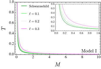
Figure 3: The Hawking temperature $T$ as a function of mass $M$ for various values of $\ell$ in Model I.

As we shall see in the evaporation subsection, the Hawking temperature derived in Eq. (66) aligns with the temperature calculated through surface gravity in Eq. (52), as expected. To provide a clearer understanding of this thermal property, its behavior is illustrated in Fig. 3, where a comparison with the standard Schwarzschild case is also presented. Generally, an increase in $\ell$ results in a higher Hawking temperature.

In other words, this implies that a black hole described by a Lorentz–violating metric radiates similarly to a greybody, with an effective temperature $T$ defined by (27).

It is essential to point out that energy conservation for the system as a whole has not been fully considered thus far. With each emission of radiation, the black hole’s total mass decreases, leading to a gradual contraction. In the following section, we will apply the tunneling method introduced by Parikh and Wilczek 011 to incorporate this effect.

III.1.2 The tunneling process

To incorporate energy conservation in calculating the radiation spectrum of our black hole solution, we employ the method presented in 011 ; vanzo2011tunnelling ; parikh2004energy ; calmet2023quantum . Adopting the Painlevé–Gullstrand form, the metric becomes $\mathrm{d}s^{2}=-\mathfrak{f}(r)\mathrm{d}t^{2}+2\mathfrak{h}(r)\mathrm{d}t\mathrm{d}r+\mathrm{d}r^{2}+r^{2}\mathrm{d}\Omega^{2}$, where $\mathfrak{h}(r)=\sqrt{\mathfrak{f}(r)\big{(}\mathfrak{g}(r)^{-1}-1\big{)}}$. The tunneling rate is linked to the imaginary part of the action parikh2004energy ; vanzo2011tunnelling ; calmet2023quantum .

The action $\mathcal{S}$ for a particle moving freely in curved spacetime can be written as $\mathcal{S}=\int p_{\mu}\,\mathrm{d}x^{\mu}$. When computing $\text{Im}\,\mathcal{S}$, only the first term in $p_{\mu}\mathrm{d}x^{\mu}=p_{t}\mathrm{d}t+p_{r}\mathrm{d}r$ contributes, as $p_{t}\mathrm{d}t=-\omega\mathrm{d}t$ remains real, leaving the imaginary component unaffected. Therefore,

$$\text{Im}\,\mathcal{S}=\text{Im}\,\int_{r_{i}}^{r_{f}}\,p_{r}\,\mathrm{d}r=\text{Im}\,\int_{r_{i}}^{r_{f}}\int_{0}^{p_{r}}\,\mathrm{d}p_{r}^{\prime}\,\mathrm{d}r.$$ (28)

Using Hamilton’s equations for a system with Hamiltonian $H=M-\omega^{\prime}$, we find that $\mathrm{d}H=-\mathrm{d}\omega^{\prime}$, where $0\leq\omega^{\prime}\leq\omega$ and $\omega$ denotes the energy of the emitted particle. Consequently, this yields:

$$\begin{split}\text{Im}\,\mathcal{S}&=\text{Im}\,\int_{r_{i}}^{r_{f}}\int_{M}^{M-\omega}\,\frac{\mathrm{d}H}{\mathrm{d}r/\mathrm{d}t}\,\mathrm{d}r\\ &=\text{Im}\,\int_{r_{i}}^{r_{f}}\,\mathrm{d}r\int_{0}^{\omega}\,-\frac{\mathrm{d}\omega^{\prime}}{\mathrm{d}r/\mathrm{d}t}\,.\end{split}$$ (29)

By rearranging the order of integration and performing the substitution

$$\frac{\mathrm{d}r}{\mathrm{d}t}=-\mathfrak{h}(r)+\sqrt{\mathfrak{f}(r)+\mathfrak{h}(r)^{2}}=1-\sqrt{\frac{\Delta(r)}{r}},$$ (30)

where $\Delta(r)=2(M-\omega^{\prime})-\frac{\ell}{1-\ell}r$. In this manner, it reads

$$\text{Im}\,\mathcal{S}=\text{Im}\,\int_{0}^{\omega}-\mathrm{d}\omega^{\prime}\int_{r_{i}}^{r_{f}}\,\frac{\mathrm{d}r}{1-\sqrt{\frac{\Delta(r,\,\omega^{\prime})}{r}}}.$$ (31)

With $M$ replaced by $(M-\omega^{\prime})$ in the original metric, the function $\Delta(r)$ now depends on $\omega^{\prime}$. This adjustment introduces a pole at the new horizon, $r=\mathfrak{r}$. Performing a contour integration around this point in the counterclockwise direction results in:

$$\text{Im}\,\mathcal{S}=4\pi(1-\ell)^{2}\omega\left(M-\frac{\omega}{2}\right).$$ (32)

According to vanzo2011tunnelling , the emission rate for a Hawking particle, incorporating Lorentz–violating corrections, can be written as

$$\Gamma\sim e^{-2\,\text{Im}\,S}=e^{-8\pi(1-\ell)^{2}\omega\left(M-\frac{\omega}{2}\right)}.$$ (33)

Notably, in the limit where $\omega\to 0$, the emission spectrum reverts to the standard Planckian form originally obtained by Hawking. Accordingly, the emission spectrum is represented by

$$\mathfrak{P}(\omega)=\frac{\mathrm{d}\omega}{2\pi}\frac{1}{e^{8\pi(1-\ell)^{2}\omega\left(M-\frac{\omega}{2}\right)}-1}.$$ (34)

The emission spectrum, with its added dependence on $\omega$, departs from the conventional blackbody distribution, a result that becomes evident upon inspection. For low $\omega$ values, the spectrum reduces to a Planck–like form but with an adjusted Hawking temperature. Furthermore, the particle number density can be formulated in terms of the tunneling rate

$$n_{1}=\frac{\Gamma}{1-\Gamma}=\frac{1}{e^{8\pi(1-\ell)^{2}\omega\left(M-\frac{\omega}{2}\right)}-1}.$$ (35)

To clarify the behavior of $n$, Fig. 1 illustrates its dependence on the Lorentz–violating parameter $\ell$. The figure confirms that an increase in $\ell$ leads to a higher particle number density. Additionally, $n_{1}$ is compared to the Schwarzschild case for reference.

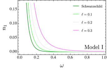
Figure 1: The particle density $n_{1}$ is shown for different values of $\ell$ in Model I.

In essence, these results suggest that radiation emitted from a black hole encodes information about its internal state. The Hawking amplitudes are affected by the Lorentz–violating parameter $\ell$, and the power spectrum incorporates these corrections, diverging from the traditional blackbody spectrum when energy conservation is taken into account.

III.2 Fermionic modes

Black holes, due to their intrinsic temperature, emit radiation akin to black body radiation, though this emission excludes adjustments for greybody factors. The resulting spectrum is predicted to contain particles of various spin types, including fermions. Studies by Kerner and Mann o69 , along with further investigations o75 ; o72 ; o71 ; o74 ; o73 ; o70 , indicate that both massless bosons and fermions emerge with the same temperature. Furthermore, research on spin–$1$ bosons has demonstrated that even when higher–order quantum corrections are applied, the Hawking temperature remains stable o77 ; o76 .

For fermions, the action is commonly represented by the phase of the spinor wave function, which satisfies the Hamilton–Jacobi equation. An alternative expression for the action is given by o83 ; o84 ; vanzo2011tunnelling

$$S_{f}=S_{0}+(\text{spin corrections}),$$

where $S_{0}$ denotes the classical action for scalar particles. The spin corrections account for the coupling between the particle’s spin and the spin connection of the manifold, yet they do not induce singularities at the horizon. It should be noted that these effects are minimal, impacting primarily the precession of spin, and can thus be disregarded here. Additionally, any impact on the black hole’s angular momentum from emitted particle spins is negligible, especially for black holes without rotation and with masses considerably larger than the Planck scale vanzo2011tunnelling . Statistically, the symmetric emission of particles with opposing spins ensures that the black hole’s angular momentum remains unchanged.

Expanding upon our previous findings, we investigate the tunneling of fermionic particles as they cross the event horizon of the specific black hole model. The emission rate is calculated within a Schwarzschild–like coordinate system, known for its singularity at the horizon. For complementary analyses utilizing generalized Painlevé–Gullstrand and Kruskal–Szekeres coordinates, refer to the foundational study o69 . As a starting point, we introduce a general metric expressed by: $\mathrm{d}s^{2}=\mathfrak{A}(r)\mathrm{d}t^{2}+[1/\mathfrak{B}(r)]\mathrm{d}r^{2}+\mathfrak{C}(r)[\mathrm{d}\theta^{2}+r^{2}\sin^{2}\theta]\mathrm{d}\varphi^{2}$. In curved spacetime, the Dirac equation is formulated as $\left(\gamma^{\mu}\nabla_{\mu}+\frac{m}{\hbar}\right)\Psi(t,r,\theta,\varphi)=0$ with $\nabla_{\mu}=\partial_{\mu}+\frac{i}{2}{\Gamma^{\alpha}_{\;\mu}}^{\;\beta}\,\Sigma_{\alpha\beta}$ and $\Sigma_{\alpha\beta}=\frac{i}{4}[\gamma_{\alpha},\gamma_{\beta}]$. The $\gamma^{\mu}$ matrices fulfill the conditions of the Clifford algebra, expressed by the relation $\{\gamma_{\alpha},\gamma_{\beta}\}=2g_{\alpha\beta}\mathbb{1}$, where $\mathbb{1}$ denotes the $4\times 4$ identity matrix. In this context, we choose the $\gamma$ matrices in the following form:

$$\gamma^{t} = \frac{i}{\sqrt{\mathfrak{A}(r)}}\left(\begin{array}[]{cc}\vec{1}&\vec{0}\\ \vec{0}&-\vec{1}\end{array}\right),\;\;\gamma^{r}=\sqrt{\mathfrak{B}(r)}\left(\begin{array}[]{cc}\vec{0}&\vec{\sigma}_{3}\\ \vec{\sigma}_{3}&\vec{0}\end{array}\right),$$

$$\gamma^{\theta} = \frac{1}{r}\left(\begin{array}[]{cc}\vec{0}&\vec{\sigma}_{1}\\ \vec{\sigma}_{1}&\vec{0}\end{array}\right),\;\;\gamma^{\varphi}=\frac{1}{r\sin\theta}\left(\begin{array}[]{cc}\vec{0}&\vec{\sigma}_{2}\\ \vec{\sigma}_{2}&\vec{0}\end{array}\right),$$

where $\vec{\sigma}$ denotes the Pauli matrices, complying with the conventional commutation: $\sigma_{i}\sigma_{j}=\vec{1}\delta_{ij}+i\varepsilon_{ijk}\sigma_{k},\,\,\text{in which}\,\,i,j,k=1,2,3.$ The matrix for $\gamma^{5}$ is instead

$$\gamma^{5}=i\gamma^{t}\gamma^{r}\gamma^{\theta}\gamma^{\varphi}=i\sqrt{\frac{\mathfrak{B}(r)}{\mathfrak{A}(r)}}\frac{1}{r^{2}\sin\theta}\left(\begin{array}[]{cc}\vec{0}&-\vec{1}\\ \vec{1}&\vec{0}\end{array}\right)\>.$$

To describe a Dirac field with spin oriented upward along the positive $r$–axis, we adopt the following ansatz vagnozzi2022horizon :

$$\Psi_{\uparrow}(t,r,\theta,\varphi)=\left(\begin{array}[]{c}\mathfrak{H}(t,r,\theta,\varphi)\\ 0\\ \mathfrak{Y}(t,r,\theta,\varphi)\\ 0\end{array}\right)\exp\left[\frac{i}{\hbar}\psi_{\uparrow}(t,r,\theta,\varphi)\right]\;.$$ (38)

We focus specifically on the spin–up ($\uparrow$) case, while noting that the spin–down ($\downarrow$) case, oriented along the negative $r$–axis, follows a similar process. Substituting the ansatz (38) into the Dirac equation results in:

$$\begin{split}-\left(\frac{i\,\mathfrak{H}}{\sqrt{\mathfrak{A}(r)}}\,\partial_{t}\psi_{\uparrow}+\mathfrak{Y}\sqrt{\mathfrak{B}(r)}\,\partial_{r}\psi_{\uparrow}\right)+\mathfrak{H}m&=0,\\ -\frac{\mathfrak{Y}}{r}\left(\partial_{\theta}\psi_{\uparrow}+\frac{i}{\sin\theta}\,\partial_{\varphi}\psi_{\uparrow}\right)&=0,\\ \left(\frac{i\,\mathfrak{Y}}{\sqrt{\mathfrak{A}(r)}}\,\partial_{t}\psi_{\uparrow}-\mathfrak{H}\sqrt{\mathfrak{B}(r)}\,\partial_{r}\psi_{\uparrow}\right)+\mathfrak{Y}m&=0,\\ -\frac{\mathfrak{H}}{r}\left(\partial_{\theta}\psi_{\uparrow}+\frac{i}{\sin\theta}\,\partial_{\varphi}\psi_{\uparrow}\right)&=0,\end{split}$$ (39)

to leading order in $\hbar$. We consider the action to be expressed as $\psi_{\uparrow}=-\omega\,t+\chi(r)+L(\theta,\varphi)$ so that the equations below are brought about vanzo2011tunnelling

$$\left(\frac{i\,\omega\,\mathfrak{H}}{\sqrt{\mathfrak{A}(r)}}-\mathfrak{Y}\sqrt{\mathfrak{B}(r)}\,\mathfrak{\chi}^{\prime}(r)\right)+m\,\mathfrak{H} = 0,$$ (40)

$$-\frac{\mathfrak{H}}{r}\left(L_{\theta}+\frac{i}{\sin\theta}L_{\varphi}\right) = 0,$$ (41)

$$-\left(\frac{i\,\omega\,\mathfrak{Y}}{\sqrt{\mathfrak{A}(r)}}+\mathfrak{H}\sqrt{\mathfrak{B}(r)}\,\mathfrak{\chi}^{\prime}(r)\right)+\mathfrak{Y}\,m = 0,$$ (42)

$$-\frac{\mathfrak{H}}{r}\left(L_{\theta}+\frac{i}{\sin\theta}L_{\varphi}\right) = 0.$$ (43)

The forms of $\mathfrak{H}$ and $\mathfrak{Y}$ do not affect the outcome that Equations (41) and (43) require $L_{\theta}+i(\sin\theta)^{-1}L_{\varphi}=0$, meaning $L(\theta,\varphi)$ must be complex. This condition for $L$ holds true for both outgoing and incoming cases. Thus, when calculating the ratio of outgoing to incoming probabilities, the contributions from $L$ cancel, allowing us to omit $L$ in further steps. In the massless scenario, Eqs. (40) and (42) provide two possible solutions:

$$\mathfrak{H}=-i\mathfrak{Y},\qquad\chi^{\prime}(r)=\chi_{\text{out}}^{\prime}=\frac{\omega}{\sqrt{\mathfrak{A}(r)\mathfrak{B}(r)}},$$ (44)

$$\mathfrak{H}=i\mathfrak{Y},\qquad\chi^{\prime}(r)=\chi_{\text{in}}^{\prime}=-\frac{\omega}{\sqrt{\mathfrak{A}(r)\mathfrak{B}(r)}},$$ (45)

where $\chi_{\text{out}}$ and $\chi_{\text{in}}$ describe the outgoing and incoming solutions, respectively vanzo2011tunnelling . Consequently, the overall tunneling probability is given by $\Gamma_{\psi}\sim e^{-2\,\text{Im}\,(\chi_{\text{out}}-\chi_{\text{in}})}$. Thereby,

$$\mathcal{\chi}_{\text{out}}(r)=-\mathcal{\chi}_{\text{in}}(r)=\int\mathrm{d}r\,\frac{\omega}{\sqrt{\mathfrak{A}(r)\mathfrak{B}(r)}}\>.$$ (46)

Notably, given the dominant energy condition and the Einstein field equations, the functions $\mathfrak{A}(r)$ and $\mathfrak{B}(r)$ share the same zeros. Thus, near $r=\mathfrak{r}$, to first order, we can express this as:

$$\mathfrak{A}(r)\mathfrak{B}(r)=\mathfrak{A}^{\prime}(\mathfrak{r})\mathfrak{B}^{\prime}(\mathfrak{r})(r-\mathfrak{r})^{2}+\dots$$ (47)

showing the presence of a simple pole with a specific coefficient. Using Feynman’s method, we obtain

$$2\mbox{ Im}\;\left(\mathcal{\chi}_{\text{out}}-\mathcal{\chi}_{\text{in}}\right)=\mbox{ Im}\int\mathrm{d}r\,\frac{4\omega}{\sqrt{\mathfrak{A}(r)\mathfrak{B}(r)}}=\frac{2\pi\omega}{\kappa},$$ (48)

with the surface gravity defined as $\kappa=\frac{1}{2}\sqrt{\mathfrak{A}^{\prime}(r_{h})\mathfrak{B}^{\prime}(r_{h})}$. Under these conditions, the expression $\Gamma_{\psi}\sim e^{-\frac{2\pi\omega}{\kappa}}$ determines the particle density $n_{\psi}$ for this black hole solution

$$n_{\psi 1}=\frac{\Gamma_{\psi}}{1+\Gamma_{\psi}}=\frac{1}{e^{8\pi(1-\ell)^{2}M\omega}+1}.$$ (49)

In Fig. 2, we illustrate the variation of $n_{\psi 1}$ across different values of $\ell$, alongside a comparison with the standard Schwarzschild case. In general lines, an increase in $\ell$ corresponds to a rise in particle density. Compared to the Lorentz–violating influenced curves, the Schwarzschild case appears as the lowest curve.

Figure 2: The particle density $n_{\psi 1}$ is shown for various values of $\ell$.

III.3 The evaporation process

Here, we examine the black hole evaporation process described by Eq. (1). This analysis utilizes the Stefan–Boltzmann law, expressed as follows:

$$\frac{\mathrm{d}M}{\mathrm{d}t}=-\alpha a\sigma T^{4},$$ (50)

where $\sigma$ denotes the cross–sectional area, $a$ is the radiation constant, and $\alpha$ represents the greybody factor. Within the geometric optics approximation, $\sigma$ is identified as the photon capture cross section, defined as follows

$$\sigma=27(1-\ell)^{3}M^{2}\pi,$$ (51)

and $T$ represents the Hawking temperature, expressed as

$$T=\frac{1}{8\pi(1-\ell)^{2}M}.$$ (52)

and, therefore,

$$\frac{\mathrm{d}M}{\mathrm{d}t}=\frac{27\xi}{4096\pi^{3}(\ell-1)^{5}M^{2}},$$ (53)

with $\xi=a\alpha$. The task now is to compute the integral below

$$\begin{split}\int_{0}^{t_{\text{evap}}}\xi\mathrm{d}\tau&=-\int_{M_{i}}^{M_{f}}\left[\frac{27}{4096\pi^{3}(1-\ell)^{5}M^{2}}\right]^{-1}\mathrm{d}M,\end{split}$$ (54)

where $t_{\text{evap}}$ represents the evaporation time. Accordingly, it is expressed as

$$t_{\text{evap}}=-\frac{4096\pi^{3}(1-\ell)^{5}\left(M_{f}^{3}-M_{i}^{3}\right)}{81\xi}.$$ (55)

Observe that $t_{\text{evap}}$ is determined through analytical calculation. For the black hole in question, no remnant mass is expected; thus, we assume it will evaporate entirely, meaning $M_{f}\to 0$, namely,

$$t_{\text{evap}}=\frac{4096\pi^{3}(1-\ell)^{5}M_{i}^{3}}{81\xi}.$$ (56)

To provide a clearer interpretation of our findings, we plot $t_{\text{evap}}$ in Fig. 4 for various values of $\ell$. It is evident that as $\ell$ increases, the evaporation time decreases.

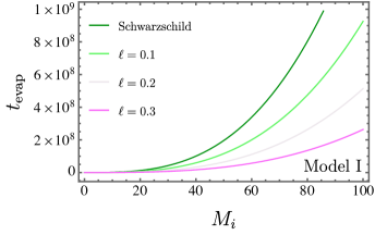
Figure 4: The evaporation time $t_{\text{evap}}$ is shown for different values of $\ell$.

IV Model II

IV.1 Bosonic modes

IV.1.1 The Hawking radiation

Similarly to the approach taken in the previous section for Model I, here, for Model II (in particular, analogous to Eq. (18) in Model I), we express

$$r_{2}=2M-\frac{E\lambda}{\sqrt{1-\ell}},$$ (57)

where we also account for the negative solution of the square root in Eq. (12) to address ingoing geodesics. Thus, we express the solution of Eq. (17) for Model II as

$$u_{2}(\lambda)=-4\sqrt{1-\ell}\,M\ln(\lambda),$$ (58)

so that

$$\mathfrak{p}_{\omega}=\int_{0}^{\infty}\left(\alpha_{\omega\omega^{\prime}}\mathfrak{f}_{\omega^{\prime}}+\beta_{\omega\omega^{\prime}}\bar{\mathfrak{f}}_{\omega^{\prime}}\right)\mathrm{d}\omega^{\prime},$$ (59)

with, for this case,

$$\begin{split}\alpha_{\omega\omega^{\prime}}=&-i\mathfrak{K}e^{i\omega^{\prime}\mathfrak{v}_{0}}e^{\pi\left[2M\sqrt{1-\ell}\right]\omega}\int_{-\infty}^{0}\,\mathrm{d}x\,\Big{(}\frac{\omega^{\prime}}{\omega}\Big{)}^{1/2}e^{\omega^{\prime}x}\\ &\times e^{i\omega\left[4M\sqrt{1-\ell}\right]\ln\left(\frac{|x|}{CD}\right)},\end{split}$$ (60)

and

$$\begin{split}\beta_{\omega\omega^{\prime}}&=i\mathfrak{K}e^{-i\omega^{\prime}\mathfrak{v}_{0}}e^{-\pi\left[2M\sqrt{1-\ell}\right]\omega}\int_{-\infty}^{0}\,\mathrm{d}x\,\left(\frac{\omega^{\prime}}{\omega}\right)^{1/2}e^{\omega^{\prime}x}\\ &\times e^{i\omega\left[4M\sqrt{1-\ell}\right]\ln\left(\frac{|x|}{CD}\right)},\end{split}$$ (61)

After some algebraic manipulations, we obtain

$$|\alpha_{\omega\omega^{\prime}}|^{2}=e^{\big{(}8\pi M\sqrt{1-\ell}\big{)}\omega}|\beta_{\omega\omega^{\prime}}|^{2}\,.$$ (62)

Analogous to the previous section, we consider $\omega$ to $\omega+\mathrm{d}\omega$ as well, leading to

$$\mathfrak{P}_{2}(\omega,\ell)=\frac{\mathrm{d}\omega}{2\pi}\frac{1}{\left\lvert\frac{\alpha_{\omega\omega^{\prime}}}{\beta_{\omega\omega^{\prime}}}\right\rvert^{2}-1}\,,$$ (63)

which follows

$$\mathfrak{P}_{2}(\omega,\ell)=\frac{\mathrm{d}\omega}{2\pi}\frac{1}{e^{\left(8\pi M\sqrt{1-\ell}\right)\omega}-1}\,.$$ (64)

When the comparison with Planck distribution is taken into account, it reads

$$\mathfrak{P}_{2}(\omega,\ell)=\frac{\mathrm{d}\omega}{2\pi}\frac{1}{e^{\frac{\omega}{T}}-1},$$ (65)

which, finally, yields

$$T_{2}=\frac{1}{8\pi\sqrt{1-\ell}\,M}.$$ (66)

As we will observe in the evaporation subsection, the Hawking temperature found in Eq. (66) aligns with that derived from surface gravity in Eq. (52), as expected. To provide a clearer understanding of this thermal quantity, its behavior is depicted in Fig. 5, along with a comparison to the Schwarzschild case. Broadly, increasing $\ell$ results in a rise in the Hawking temperature. Additionally, consistent with the findings of the previous section, there is no remnant mass in this scenario.

As in Model I, since the black hole radiates, its mass steadily decreases, leading to its gradual reduction. In the following section, we shall apply the tunneling approach developed by Parikh and Wilczek 011 to model this effect, similar to our treatment for Model I.

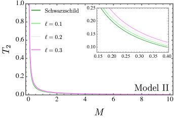
Figure 5: The Hawking temperature $T_{2}$ as a function of mass $M$ for various values of $\ell$ in Model II.

IV.1.2 The tunneling process

Following the approach taken in the previous section for Model I, here we consider $\Delta(r)=\frac{-\ell r+2M}{1-\ell}$ so that the integral in Eq. (67) can be evaluated as shown below

$$\text{Im}\,\mathcal{S}=\text{Im}\,\int_{0}^{\omega}-\mathrm{d}\omega^{\prime}\int_{r_{i}}^{r_{f}}\,\frac{\mathrm{d}r}{\sqrt{1-\ell}\left(1-\sqrt{\frac{\Delta(r)}{r}}\right)}.$$ (67)

The function $\Delta(r)$ will depend on $\omega^{\prime}$, resulting from substituting $M$ with $(M-\omega^{\prime})$ in the metric. This modification creates a pole at the new horizon location $r=\mathfrak{r}$. Integrating along a counterclockwise path around this pole produces

$$\text{Im}\,\mathcal{S}=4\pi\sqrt{1-\ell}\,\omega\left(M-\frac{\omega}{2}\right).$$ (68)

Thus, the Lorentz–violating correction to the emission rate for a Hawking particle is given by

$$\Gamma_{2}\sim e^{-2\,\text{Im}\,S}=e^{-8\pi\sqrt{1-\ell}\,\omega\left(M-\frac{\omega}{2}\right)}.$$ (69)

Notably, in the limit $E\to 0$, the standard Planckian spectrum as initially derived by Hawking is restored. Consequently, the emission spectrum is given by

$$\mathfrak{P}_{2}(\omega)=\frac{\mathrm{d}\omega}{2\pi}\frac{1}{e^{8\pi\sqrt{1-\ell}\,\omega\left(M-\frac{\omega}{2}\right)}-1}.$$ (70)

With its additional dependence on $\omega$, the emission spectrum departs from the classic black body distribution, as can be readily observed. For small values of $\omega$, the expression reduces to the Planck distribution but with an adjusted Hawking temperature. Furthermore, the particle number density can be determined using the tunneling rate

$$n_{2}=\frac{\Gamma_{2}}{1-\Gamma_{2}}=\frac{1}{e^{8\pi\sqrt{1-\ell}\,\omega\left(M-\frac{\omega}{2}\right)}-1}$$ (71)

To provide a clearer understanding of $n_{2}$, we present Fig. 6, which illustrates its dependence on the Lorentz-violating parameter $\ell$. As $\ell$ increases, we observe an increase in particle number density. Additionally, $n_{2}$ is compared with the Schwarzschild case. In contrast to $n_{1}$, the lines representing $n_{2}$ are spaced more closely together.

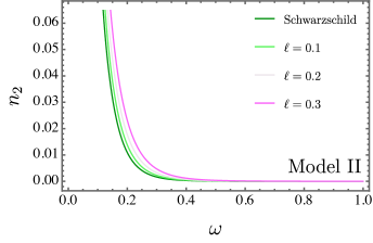
Figure 6: The particle density $n_{2}$ is shown for different values of $\ell$ in Model II.

We further compare the particle density for both models developed here in the bosonic case, denoted by $n_{1}$ and $n_{2}$, in Fig. 7. The Schwarzschild case is also included for reference. In a general panorama, the particle density intensities exhibit the following hierarchy: $n$ (Model I) $>n_{2}$ (Model II) $>$ Schwarzschild.

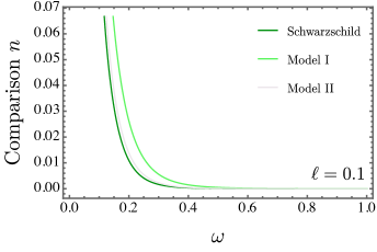
Figure 7: Comparison of $n$ for Model I and Model II with $\ell=0.1$ and $M=1$, alongside the Schwarzschild case.

IV.2 Fermionic modes

Using all definitions outlined thus far, we can now express the particle density for fermions in Model II as follows:

$$n_{\psi 2}=\frac{\Gamma_{\psi 2}}{1+\Gamma_{\psi 2}}=\frac{1}{e^{\frac{8\pi\omega}{\sqrt{\frac{1}{M^{2}-\ell M^{2}}}}}+1}.$$ (72)

In Fig. 8, we illustrate the behavior of $n_{\psi 2}$ across different values of $\ell$ and compare these findings with the standard Schwarzschild case. Additionally, Fig. 9 compares both models with the Schwarzschild case. Overall, we observe that Model I exhibits a higher particle density than Model II. It is also important to note that the Schwarzschild case shows the lowest particle density among them.

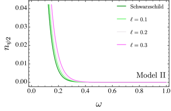
Figure 8: The particle density $n_{\psi 2}$ is shown for different values of $\ell$ in Model II.

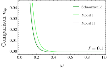
Figure 9: Comparison of $n_{\psi}$ for Model I and Model II with $\ell=0.1$ and $M=1$, alongside the Schwarzschild case.

IV.3 The evaporation process

In Model II, the Lorentz violation parameter $\ell$ has no effect on the event horizon, photon sphere, or shadow radii. However, it does modify the Hawking temperature, leading to a difference in the evaporation process when compared to the Schwarzschild case. Thus, we express

$$T_{2}=\frac{1}{8\pi\sqrt{1-\ell}\,M}.$$

As in the previous section, we will apply the Stefan–Boltzmann law from Eq. (50) to analyze the black hole evaporation process. Here, we set $\sigma=\pi(3\sqrt{3}M)^{2}$, yielding

$$\begin{split}\int_{0}^{t_{\text{evap2}}}\xi\mathrm{d}\tau&=-\int_{M_{i}}^{M_{f}}\left[\frac{27\xi}{4096\pi^{3}(1-\ell)^{2}M^{2}}\right]^{-1}\mathrm{d}M.\end{split}$$ (73)

Accordingly, it is given by

$$t_{\text{evap2}}=-\frac{4096\pi^{3}(1-\ell)^{2}\left(M_{f}^{3}-M_{i}^{3}\right)}{81\xi}.$$ (74)

For this black hole model, analogous to the Model I, no remnant mass is expected; thus, we assume it will evaporate completely, meaning $M_{f}\to 0$.

$$t_{\text{evap2}}=\frac{4096\pi^{3}(1-\ell)^{2}M_{i}^{3}}{81\xi}.$$ (75)

To clarify our results, we plot $t_{\text{evap2}}$ in Fig. 10 for various values of $\ell$. As $\ell$ increases, evaporation time decreases. For a comparative analysis of the two models developed thus far, we present

$$\frac{t_{\text{evap}}}{t_{\text{evap2}}}=(1-\ell)^{3}.$$ (76)

This indicates that the evaporation time for Model I is shorter than for Model II, since $\ell\ll 0$ Junior:2024ety . Consequently, Model I undergoes evaporation more rapidly than Model II. To illustrate this difference, we plot both models at a fixed value of $\ell=0.1$ to directly compare their evaporation times. This is shown in Fig. 11. Overall, both Models I and II exhibit faster evaporation rates than the Schwarzschild case. However, between the two, Model I consistently evaporates faster than Model II.

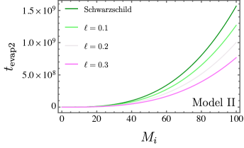
Figure 10: The evaporation time $t_{\text{evap}}$ is shown for different values of $\ell$.

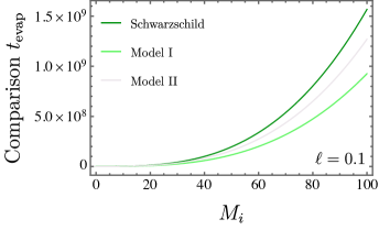
Figure 11: Comparison of the evaporation time $t_{\text{evap}}$ for Model I and Model II when a fixed value of $\ell=0.1$ is considered.

V Conclusion

In this paper, we examined particle creation and the evaporation process within Kalb–Ramond gravity, employing two solutions from the literature, denoted here as Model I yang2023static and Model II Liu:2024oas .

Starting with Model I, we focused on bosonic modes, quantizing the scalar field in curved spacetime to address Hawking radiation. This allowed us to calculate the Hawking temperature, $T$, using Bogoliubov coefficients, observing that increasing $\ell$ led to a higher temperature. We then explored Hawking radiation through the tunneling process, factoring in energy conservation. Our findings showed that the emission spectra deviated from the typical black body radiation due to Lorentz–violating corrections associated with $\ell$. The resulting particle number density, $n_{1}$, demonstrated that increasing $\ell$ also increased particle density. Fermionic modes were subsequently considered, yielding the particle density $n_{\psi 1}$. Similar to the bosonic case, $n_{\psi 1}$ increased with $\ell$. Lastly, the evaporation process for Model I revealed that a larger Lorentz–violating parameter $\ell$ shortened the black hole’s lifetime $t_{\text{evap}}$, which was derived analytically.

For Model II, we followed a similar approach, analyzing both bosonic and fermionic modes along with the evaporation process. Here, the Hawking temperature $T_{2}$ was obtained through the Klein–Gordon equation in curved spacetime, again showing an increase in temperature with $\ell$. The tunneling process also yielded particle densities $n_{2}$ for bosons and $n_{\psi 2}$ for fermions, both of which increased as $\ell$ grew. The evaporation process for showed that $t_{\text{evap2}}$ decreased with increasing $\ell$, mirroring Model I’s behavior.

Comparing the two models, particle densities $n_{1}$ and $n_{2}$ (bosonic) and $n_{\psi 1}$ and $n_{\psi 2}$ (fermionic) were found to be higher in Model I than in Model II, and both models produced higher densities than the Schwarzschild case. In terms of evaporation time, Model I had a shorter lifetime than Model II, as $\ell\ll 0$. While both models evaporate faster than the Schwarzschild black hole, Model I consistently exhibits a more rapid evaporation rate than Model II.

As a future perspective, our investigation can be extended to include two new solutions within the framework of effective quantum gravity, as presented in Ref. zhang2024black . This and other Lorentz–violating extensions are currently under development.

VI Data Availability Statement

Data Availability Statement: No Data associated in the manuscript

References

- (1) K. Yang, Y.-Z. Chen, Z.-Q. Duan, and J.-Y. Zhao, “Static and spherically symmetric black holes in gravity with a background kalb-ramond field,” Physical Review D, vol. 108, no. 12, p. 124004, 2023.
- (2) W. Liu, D. Wu, and J. Wang, “Static neutral black holes in Kalb-Ramond gravity,” JCAP, vol. 09, p. 017, 2024.
- (3) J. Alfaro, H. Morales-Tecotl, and L. Urrutia, “Loop quantum gravity and light propagation,” Phys. Rev. D, vol. 65, p. 103509, 2002.
- (4) V. Kostelecky and S. Samuel, “Spontaneous breaking of lorentz symmetry in string theory,” Phys. Rev. D, vol. 39, p. 683, 1989.
- (5) S. Carroll, J. Harvey, V. Kostelecky, C. Lane, and T. Okamoto, “Noncommutative field theory and lorentz violation,” Phys. Rev. Lett., vol. 87, p. 141601, 2001.
- (6) A. A. Araújo Filho, S. Zare, P. J. Porfírio, J. Kriz, and H. Hassanabadi, “Thermodynamics and evaporation of a modified schwarzschild black hole in a non–commutative gauge theory,” Physics Letters B, vol. 838, p. 137744, 2023.
- (7) N. Heidari, H. Hassanabadi, A. A. Araújo Filho, J. Kriz, S. Zare, and P. J. Porfírio, “Gravitational signatures of a non–commutative stable black hole,” Physics of the Dark Universe, p. 101382, 2023.
- (8) P. Horava, “Quantum gravity at a lifshitz point,” Phys. Rev., vol. 79, p. 084008, 2009.
- (9) S. Dubovsky, P. Tinyakov, and I. Tkachev, “Massive graviton as a testable cold dark matter candidate,” Phys. Rev. Lett., vol. 94, p. 181102, 2005.
- (10) T. Jacobson and D. Mattingly, “Gravity with a dynamical preferred frame,” Phys. Rev. D, vol. 64, p. 024028, 2001.
- (11) A. Cohen and S. Glashow, “Very special relativity,” Phys. Rev. Lett., vol. 97, p. 021601, 2006.
- (12) G. Bengochea and R. Ferraro, “Dark torsion as the cosmic speed-up,” Phys. Rev. D, vol. 79, p. 124019, 2009.
- (13) R. Bluhm, “Overview of the standard model extension: implications and phenomenology of lorentz violation,” in Special Relativity: Will it Survive the Next 101 Years?, pp. 191–226, Springer, 2006.
- (14) R. Bluhm, S.-H. Fung, and V. A. Kosteleckỳ, “Spontaneous lorentz and diffeomorphism violation, massive modes, and gravity,” Physical Review D, vol. 77, no. 6, p. 065020, 2008.
- (15) Q. Bailey and V. Kostelecky, “Signals for lorentz violation in post-newtonian gravity,” Phys. Rev. D, vol. 74, p. 045001, 2006.
- (16) M. Khodadi and M. Schreck, “Hubble tension as a guide for refining the early universe: Cosmologies with explicit local lorentz and diffeomorphism violation,” Physics of the Dark Universe, vol. 39, p. 101170, 2023.
- (17) A. A. Araújo Filho, J. R. Nascimento, A. Y. Petrov, and P. J. Porfírio, “An exact stationary axisymmetric vacuum solution within a metric-affine bumblebee gravity,” JCAP, vol. 07, p. 004, 2024.
- (18) R. Bluhm, N. Gagne, R. Potting, and A. Vrublevskis, “Constraints and stability in vector theories with spontaneous lorentz violation,” Phys. Rev. D, vol. 77, p. 125007, 2008.
- (19) V. Kostelecky and S. Samuel, “Phenomenological gravitational constraints on strings and higher dimensional theories,” Phys. Rev. Lett., vol. 63, p. 224, 1989.
- (20) V. Kostelecky, “Gravity, lorentz violation, and the standard model,” Phys. Rev. D, vol. 69, p. 105009, 2004.
- (21) V. Kostelecky and S. Samuel, “Gravitational phenomenology in higher dimensional theories and strings,” Phys. Rev. D, vol. 40, p. 1886, 1989.
- (22) A. A. Araújo Filho, J. R. Nascimento, A. Y. Petrov, and P. J. Porfírio, “Vacuum solution within a metric-affine bumblebee gravity,” Physical Review D, vol. 108, no. 8, p. 085010, 2023.
- (23) M. Khodadi, G. Lambiase, and L. Mastrototaro, “Spontaneous lorentz symmetry breaking effects on grbs jets arising from neutrino pair annihilation process near a black hole,” The European Physical Journal C, vol. 83, no. 3, p. 239, 2023.
- (24) M. Khodadi, G. Lambiase, and A. Sheykhi, “Constraining the lorentz-violating bumblebee vector field with big bang nucleosynthesis and gravitational baryogenesis,” The European Physical Journal C, vol. 83, no. 5, p. 386, 2023.
- (25) S. Capozziello, S. Zare, D. Mota, and H. Hassanabadi, “Dark matter spike around bumblebee black holes,” Journal of Cosmology and Astroparticle Physics, vol. 2023, no. 05, p. 027, 2023.
- (26) M. Khodadi, “Magnetic reconnection and energy extraction from a spinning black hole with broken lorentz symmetry,” Physical Review D, vol. 105, no. 2, p. 023025, 2022.
- (27) A. A. Araújo Filho, “Lorentz-violating scenarios in a thermal reservoir,” The European Physical Journal Plus, vol. 136(4), 417 (2021).
- (28) A. A. Araújo Filho, J. Furtado, H. Hassanabadi, and J. Reis, “Thermal analysis of photon–like particles in rainbow gravity,” Physics of Dark Universe, vol. 42, no. 8, p. 101310, 2023.
- (29) A. A. Araújo Filho, “Particles in loop quantum gravity formalism: a thermodynamical description,” Annalen der Physik, p. 2200383, 2022.
- (30) A. A. Araújo Filho and A. Y. Petrov, “Higher-derivative lorentz-breaking dispersion relations: a thermal description,” The European Physical Journal C, vol. 81(9), 843 (2021).
- (31) A. A. Araújo Filho and R. V. Maluf, “Thermodynamic properties in higher-derivative electrodynamics,” Brazilian Journal of Physics, vol. 51, no. 3, pp. 820–830, 2021.
- (32) A. A. Araújo Filho and J. Reis, “How does geometry affect quantum gases?,” International Journal of Modern Physics A, vol. 37, no. 11n12, p. 2250071, 2022.
- (33) A. A. Araújo Filho, “Thermodynamics of massless particles in curved spacetime,” arXiv preprint arXiv:2201.00066, 2021.
- (34) M. Anacleto, F. Brito, E. Maciel, A. Mohammadi, E. Passos, W. Santos, and J. Santos, “Lorentz-violating dimension-five operator contribution to the black body radiation,” Physics Letters B, vol. 785, pp. 191–196, 2018.
- (35) A. A. Araújo Filho and A. Y. Petrov, “Bouncing universe in a heat bath,” International Journal of Modern Physics A, vol. 36, no. 34 & 35, (2021) 2150242. DOI: doi.org/10.1142/S0217751X21502420.
- (36) J. Reis et al., “Thermal aspects of interacting quantum gases in lorentz-violating scenarios,” The European Physical Journal Plus, vol. 136, no. 3, pp. 1–30, 2021.
- (37) A. A. Araújo Filho, Thermal aspects of field theories. Amazon. com, 2022.
- (38) R. Casana, A. Cavalcante, F. Poulis, and E. Santos, “Exact schwarzschild-like solution in a bumblebee gravity model,” Phys. Rev., vol. 97, p. 104001, 2018.
- (39) A. Ovgun, K. Jusufi, and I. Sakalli, “Gravitational lensing under the effect of weyl and bumblebee gravities: Applications of gauss-bonnet theorem,” Annals Phys., vol. 399, p. 193, 2018.
- (40) Z. Cai and R.-J. Yang, “Accretion of the vlasov gas onto a schwarzschild-like black hole,”
- (41) R.-J. Yang, H. Gao, Y. Zheng, and Q. Wu, “Effects of lorentz breaking on the accretion onto a schwarzschild-like black hole,” Commun. Theor. Phys., vol. 71, p. 568, 2019.
- (42) R. Oliveira, D. Dantas, and C. Almeida, “Quasinormal frequencies for a black hole in a bumblebee gravity,” EPL, vol. 135, p. 10003, 2021.
- (43) S. Kanzi and İ. Sakallı, “Gup modified hawking radiation in bumblebee gravity,” Nuclear Physics B, vol. 946, p. 114703, 2019.
- (44) R. Maluf and J. Neves, “Black holes with a cosmological constant in bumblebee gravity,” Phys. Rev. D, vol. 103, p. 044002, 2021.
- (45) D. Liang, R. Xu, Z.-F. Mai, and L. Shao, “Probing vector hair of black holes with extreme-mass-ratio inspirals,” Phys. Rev. D, vol. 107, p. 044053, 2023.
- (46) R. Xu, D. Liang, and L. Shao, “Bumblebee black holes in light of event horizon telescope observations,” Astrophys. J., vol. 945, p. 148, 2023.
- (47) Z.-F. Mai, R. Xu, D. Liang, and L. Shao, “Extended thermodynamics of the bumblebee black holes,” Phys. Rev. D, vol. 108, p. 024004, 2023.
- (48) R. Xu, D. Liang, and L. Shao, “Static spherical vacuum solutions in the bumblebee gravity model,” Phys. Rev. D, vol. 107, p. 024011, 2023.
- (49) B. Altschul, Q. Bailey, and V. Kostelecky, “Lorentz violation with an antisymmetric tensor,” Phys. Rev. D, vol. 81, p. 065028, 2010.
- (50) R. Maluf, A. A. Araújo Filho, W. Cruz, and C. Almeida, “Antisymmetric tensor propagator with spontaneous lorentz violation,” Europhysics Letters, vol. 124, p. 61001, 2019.
- (51) M. Kalb and P. Ramond, “Classical direct interstring action,” Phys. Rev. D, vol. 9, p. 2273, 1974.
- (52) L. Lessa, J. Silva, R. Maluf, and C. Almeida, “Modified black hole solution with a background kalb-ramond field,” Eur. Phys. J. C, vol. 80, p. 335, 2020.
- (53) F. Atamurotov, D. Ortiqboev, A. Abdujabbarov, and G. Mustafa, “Particle dynamics and gravitational weak lensing around black hole in the kalb-ramond gravity,” Eur. Phys. J. C, vol. 82, p. 659, 2022.
- (54) R. Kumar, S. Ghosh, and A. Wang, “Gravitational deflection of light and shadow cast by rotating kalb-ramond black holes,” Phys. Rev. D, vol. 101, p. 104001, 2020.
- (55) S. W. Hawking, “Particle creation by black holes,” Communications in mathematical physics, vol. 43, no. 3, pp. 199–220, 1975.
- (56) S. W. Hawking, “Black hole explosions?,” Nature, vol. 248, no. 5443, pp. 30–31, 1974.
- (57) S. W. Hawking, “Black holes and thermodynamics,” Physical Review D, vol. 13, no. 2, p. 191, 1976.
- (58) A. Övgün and I. Sakallı, “Hawking Radiation via Gauss-Bonnet Theorem,” Annals Phys., vol. 413, p. 168071, 2020.
- (59) G. W. Gibbons and S. W. Hawking, “Cosmological event horizons, thermodynamics, and particle creation,” Physical Review D, vol. 15, no. 10, p. 2738, 1977.
- (60) X.-M. Kuang, J. Saavedra, and A. Övgün, “The Effect of the Gauss-Bonnet term to Hawking Radiation from arbitrary dimensional Black Brane,” Eur. Phys. J. C, vol. 77, no. 9, p. 613, 2017.
- (61) X.-M. Kuang, B. Liu, and A. Övgün, “Nonlinear electrodynamics AdS black hole and related phenomena in the extended thermodynamics,” Eur. Phys. J. C, vol. 78, no. 10, p. 840, 2018.
- (62) A. Övgün, I. Sakallı, J. Saavedra, and C. Leiva, “Shadow cast of noncommutative black holes in Rastall gravity,” Mod. Phys. Lett. A, vol. 35, no. 20, p. 2050163, 2020.
- (63) A. Övgün and K. Jusufi, “Massive vector particles tunneling from noncommutative charged black holes and their GUP-corrected thermodynamics,” Eur. Phys. J. Plus, vol. 131, no. 5, p. 177, 2016.
- (64) P. Sedaghatnia, H. Hassanabadi, P. J. Porfírio, W. S. Chung, et al., “Thermodynamical properties of a deformed schwarzschild black hole via dunkl generalization,” arXiv preprint arXiv:2302.11460, 2023.
- (65) A. Jawad and A. Khawer, “Thermodynamic consequences of well-known regular black holes under modified first law,” The European Physical Journal C, vol. 78, pp. 1–10, 2018.
- (66) D. Hansen, D. Kubizňák, and R. B. Mann, “Criticality and surface tension in rotating horizon thermodynamics,” Classical and Quantum Gravity, vol. 33, no. 16, p. 165005, 2016.
- (67) A. A. Araújo Filho, K. Jusufi, B. Cuadros-Melgar, and G. Leon, “Dark matter signatures of black holes with yukawa potential,” Physics of the Dark Universe, vol. 44, p. 101500, 2024.
- (68) C. Vaz, “Canonical quantization and the statistical entropy of the schwarzschild black hole,” Physical Review D, vol. 61, no. 6, p. 064017, 2000.
- (69) B. Harms and Y. Leblanc, “Statistical mechanics of black holes,” Physical Review D, vol. 46, no. 6, p. 2334, 1992.
- (70) D. Chen, J. Tao, et al., “The modified first laws of thermodynamics of anti-de sitter and de sitter space–times,” Nuclear Physics B, vol. 918, pp. 115–128, 2017.
- (71) A. A. Araújo Filho, “Implications of a simpson–visser solution in verlinde’s framework,” The European Physical Journal C, vol. 84, no. 1, pp. 1–22, 2024.
- (72) A. A. Araújo Filho, “Analysis of a regular black hole in verlinde’s gravity,” Classical and Quantum Gravity, vol. 41, no. 1, p. 015003, 2023.
- (73) D. Hansen, D. Kubizňák, and R. B. Mann, “Universality of p- v criticality in horizon thermodynamics,” Journal of High Energy Physics, vol. 2017, no. 1, pp. 1–24, 2017.
- (74) P. Kraus and F. Wilczek, “Self-interaction correction to black hole radiance,” Nuclear Physics B, vol. 433, no. 2, pp. 403–420, 1995.
- (75) M. K. Parikh, “Energy conservation and hawking radiation,” arXiv preprint hep-th/0402166, 2004.
- (76) M. Parikh, “A secret tunnel through the horizon,” International Journal of Modern Physics D, vol. 13, no. 10, pp. 2351–2354, 2004.
- (77) M. K. Parikh and F. Wilczek, “Hawking radiation as tunneling,” Physical review letters, vol. 85, no. 24, p. 5042, 2000.
- (78) G. Johnson and J. March-Russell, “Hawking radiation of extended objects,” Journal of High Energy Physics, vol. 2020, no. 4, pp. 1–16, 2020.
- (79) D. Senjaya, “The bocharova–bronnikov–melnikov–bekenstein black hole’s exact quasibound states and hawking radiation,” The European Physical Journal C, vol. 84, no. 6, p. 607, 2024.
- (80) L. Vanzo, G. Acquaviva, and R. Di Criscienzo, “Tunnelling methods and hawking’s radiation: achievements and prospects,” Classical and Quantum Gravity, vol. 28, no. 18, p. 183001, 2011.
- (81) X. Calmet, S. D. Hsu, and M. Sebastianutti, “Quantum gravitational corrections to particle creation by black holes,” Physics Letters B, vol. 841, p. 137820, 2023.
- (82) F. Mirekhtiary, A. Abbasi, K. Hosseini, and F. Tulucu, “Tunneling of rotational black string with nonlinear electromagnetic fields,” Physica Scripta, vol. 99, no. 3, p. 035005, 2024.
- (83) M. Anacleto, F. Brito, and E. Passos, “Quantum-corrected self-dual black hole entropy in tunneling formalism with gup,” Physics Letters B, vol. 749, pp. 181–186, 2015.
- (84) P. Mitra, “Hawking temperature from tunnelling formalism,” Physics Letters B, vol. 648, no. 2-3, pp. 240–242, 2007.
- (85) C. Silva and F. Brito, “Quantum tunneling radiation from self-dual black holes,” Physics Letters B, vol. 725, no. 4-5, pp. 456–462, 2013.
- (86) A. Medved, “Radiation via tunneling from a de sitter cosmological horizon,” Physical Review D, vol. 66, no. 12, p. 124009, 2002.
- (87) F. Del Porro, S. Liberati, and M. Schneider, “Tunneling method for hawking quanta in analogue gravity,” arXiv preprint arXiv:2406.14603, 2024.
- (88) J. Zhang and Z. Zhao, “New coordinates for kerr–newman black hole radiation,” Physics Letters B, vol. 618, no. 1-4, pp. 14–22, 2005.
- (89) A. Touati and Z. Slimane, “Quantum tunneling from schwarzschild black hole in non-commutative gauge theory of gravity,” Physics Letters B, vol. 848, p. 138335, 2024.
- (90) A. A. Araújo Filho, J. A. A. S. Reis, and H. Hassanabadi, “Exploring antisymmetric tensor effects on black hole shadows and quasinormal frequencies,” Journal of Cosmology and Astroparticle Physics, vol. 2024, no. 05, p. 029, 2024.
- (91) W.-D. Guo, Q. Tan, and Y.-X. Liu, “Quasinormal modes and greybody factor of a lorentz-violating black hole,” Journal of Cosmology and Astroparticle Physics, vol. 2024, no. 07, p. 008, 2024.
- (92) E. L. B. Junior, J. T. S. S. Junior, F. S. N. Lobo, M. E. Rodrigues, D. Rubiera-Garcia, L. F. D. da Silva, and H. A. Vieira, “Gravitational lensing of a schwarzschild-like black hole in kalb-ramond gravity,” Physical Review D, vol. 110, no. 2, p. 024077, 2024.
- (93) E. L. B. Junior, J. T. S. S. Junior, F. S. N. Lobo, M. E. Rodrigues, D. Rubiera-Garcia, L. F. D. da Silva, and H. A. Vieira, “Spontaneous lorentz symmetry-breaking constraints in kalb-ramond gravity,” arXiv preprint arXiv:2405.03291, 2024.
- (94) S. Jumaniyozov, S. U. Khan, J. Rayimbaev, A. Abdujabbarov, S. Urinbaev, and S. Murodov, “Circular motion and qpos near black holes in kalb–ramond gravity,” The European Physical Journal C, vol. 84, no. 9, p. 964, 2024.
- (95) Y.-H. Jiang and X. Zhang, “Accretion of vlasov gas onto a black hole in the kalb–ramond field,” Chinese Physics C, 2024.
- (96) Z.-Q. Duan, J.-Y. Zhao, and K. Yang, “Electrically charged black holes in gravity with a background kalb–ramond field,” The European Physical Journal C, vol. 84, no. 8, p. 798, 2024.
- (97) N. Heidari, J. A. A. S. Reis, H. Hassanabadi, et al., “The impact of an antisymmetric tensor on charged black holes: evaporation process, geodesics, deflection angle, scattering effects and quasinormal modes,” arXiv preprint arXiv:2404.10721, 2024.
- (98) A. al Badawi, S. Shaymatov, and I. Sakallı, “Geodesics structure and deflection angle of electrically charged black holes in gravity with a background Kalb–Ramond field,” Eur. Phys. J. C, vol. 84, no. 8, p. 825, 2024.
- (99) A. A. Araújo Filho, “Antisymmetric tensor influence on charged black hole lensing phenomena and time delay,” arXiv preprint arXiv:2406.11582, 2024.
- (100) M. Zahid, J. Rayimbaev, N. Kurbonov, S. Ahmedov, C. Shen, and A. Abdujabbarov, “Electric Penrose, circular orbits and collisions of charged particles near charged black holes in Kalb–Ramond gravity,” Eur. Phys. J. C, vol. 84, no. 7, p. 706, 2024.
- (101) H. Chen, M. Zhang, F. Hosseinifar, H. Hassanabadi, et al., “Thermal, topological, and scattering effects of an ads charged black hole with an antisymmetric tensor background,” arXiv preprint arXiv:2408.03090, 2024.
- (102) F. Hosseinifar, M. Zhang, H. Chen, H. Hassanabadi, et al., “Shadows, greybody factors, emission rate, topological charge, and phase transitions for a charged black hole with a kalb-ramond field background,” arXiv preprint arXiv:2407.07017, 2024.
- (103) W. Liu, C. Wen, and J. Wang, “Lorentz violation alleviates gravitationally induced entanglement degradation,” arXiv preprint arXiv:2410.21681, 2024.
- (104) S. W. Hawking, “Particle creation by black holes,” in Euclidean quantum gravity, pp. 167–188, World Scientific, 1975.
- (105) A. A. Araújo Filho, N. Heidari, and A. Övgün, “Quantum gravity effects on particle creation and evaporation in a non-commutative black hole via mass deformation,” arXiv preprint arXiv:2409.03566, 2024.
- (106) L. Parker and D. Toms, Quantum field theory in curved spacetime: quantized fields and gravity. Cambridge university press, 2009.
- (107) S. Hollands and R. M. Wald, “Quantum fields in curved spacetime,” Physics Reports, vol. 574, pp. 1–35, 2015.
- (108) R. M. Wald, Quantum field theory in curved spacetime and black hole thermodynamics. University of Chicago press, 1994.
- (109) S. A. Fulling, Aspects of quantum field theory in curved spacetime. No. 17, Cambridge university press, 1989.
- (110) M. K. Parikh, “Energy conservation and hawking radiation,” arXiv preprint hep-th/0402166, 2004.
- (111) R. Kerner and R. B. Mann, “Fermions tunnelling from black holes,” Classical and Quantum Gravity, vol. 25, no. 9, p. 095014, 2008.
- (112) M. Rehman and K. Saifullah, “Charged fermions tunneling from accelerating and rotating black holes,” Journal of Cosmology and Astroparticle Physics, vol. 2011, no. 03, p. 001, 2011.
- (113) H.-L. Li, S.-Z. Yang, T.-J. Zhou, and R. Lin, “Fermion tunneling from a vaidya black hole,” Europhysics Letters, vol. 84, no. 2, p. 20003, 2008.
- (114) R. Di Criscienzo and L. Vanzo, “Fermion tunneling from dynamical horizons,” Europhysics Letters, vol. 82, no. 6, p. 60001, 2008.
- (115) A. Yale and R. B. Mann, “Gravitinos tunneling from black holes,” Physics Letters B, vol. 673, no. 2, pp. 168–172, 2009.
- (116) R. Kerner and R. B. Mann, “Charged fermions tunnelling from kerr–newman black holes,” Physics letters B, vol. 665, no. 4, pp. 277–283, 2008.
- (117) A. Yale, “Exact hawking radiation of scalars, fermions, and bosons using the tunneling method without back-reaction,” Physics Letters B, vol. 697, no. 4, pp. 398–403, 2011.
- (118) A. Yale, “There are no quantum corrections to the hawking temperature via tunneling from a fixed background,” The European Physical Journal C, vol. 71, pp. 1–4, 2011.
- (119) B. Chatterjee and P. Mitra, “Hawking temperature and higher order calculations,” Physics Letters B, vol. 675, no. 2, pp. 240–242, 2009.
- (120) A. Barducci, R. Casalbuoni, and L. Lusanna, “Supersymmetries and the pseudoclassical relativistic electron,” Nuovo Cimento. A, vol. 35, no. 3, pp. 377–399, 1976.
- (121) G. Cognola, L. Vanzo, S. Zerbini, and R. Soldati, “On the lagrangian formulation of a charged spinning particle in an external electromagnetic field,” Physics Letters B, vol. 104, no. 1, pp. 67–69, 1981.
- (122) S. Vagnozzi, R. Roy, Y.-D. Tsai, L. Visinelli, M. Afrin, A. Allahyari, P. Bambhaniya, D. Dey, S. G. Ghosh, P. S. Joshi, et al., “Horizon-scale tests of gravity theories and fundamental physics from the event horizon telescope image of sagittarius a,” Classical and Quantum Gravity, 2022.
- (123) E. L. B. Junior, J. T. S. S. Junior, F. S. N. Lobo, M. E. Rodrigues, D. Rubiera-Garcia, L. F. D. da Silva, and H. A. Vieira, “Spontaneous Lorentz symmetry-breaking constraints in Kalb-Ramond gravity,” 5 2024.
- (124) C. Zhang, J. Lewandowski, Y. Ma, and J. Yang, “Black holes and covariance in effective quantum gravity,” arXiv preprint arXiv:2407.10168, 2024.