Spatially Constrained Transformer with Efficient Global Relation Modelling for Spatio-Temporal Prediction
Abstract
Accurate spatio-temporal prediction is crucial for the sustainable development of smart cities. However, current approaches often struggle to capture important spatio-temporal relationships, particularly overlooking global relations among distant city regions. Most existing techniques predominantly rely on Convolutional Neural Networks (CNNs) to capture global relations. However, CNNs exhibit neighbourhood bias, making them insufficient for capturing distant relations. To address this limitation, we propose ST-SampleNet, a novel transformer-based architecture that combines CNNs with self-attention mechanisms to capture both local and global relations effectively. Moreover, as the number of regions increases, the quadratic complexity of self-attention becomes a challenge. To tackle this issue, we introduce a lightweight region sampling strategy that prunes non-essential regions and enhances the efficiency of our approach. Furthermore, we introduce a spatially constrained position embedding that incorporates spatial neighbourhood information into the self-attention mechanism, aiding in semantic interpretation and improving the performance of ST-SampleNet. Our experimental evaluation on three real-world datasets demonstrates the effectiveness of ST-SampleNet. Additionally, our efficient variant achieves a reduction in computational costs with only a marginal compromise in performance, approximately .
2055
1 Introduction
Spatio-temporal prediction aims to predict future spatio-temporal dynamics based on historical data. This prediction task is commonly categorised into two domains: road network-level predictions [23, 13, 5], often modelled as graph-based problems, and region-level predictions [35, 17], typically approached as grid-based problems. This paper addresses region-level prediction, emphasising its significance for city planners, administrators, and ride-hailing companies. Focusing on this level is crucial for informed decision-making in smart city planning and development [8]. Accurate region-level prediction enables one to view city-wide traffic dynamics, which helps in the sustainable development of cities to provide better access to transport and public services.
For accurate spatio-temporal prediction, three essential spatio-temporal relations need to be addressed:
-
•
Local Spatial Relations between closed neighbouring regions. For example, congestion in one region often affects adjacent regions due to the interconnectedness of road networks.
-
•
Global Spatial Relations between distant regions. For instance, distant residential areas often share similar traffic patterns, such as peak traffic during morning and evening rush hours.
-
•
Temporal Relations between input time intervals. For example, traffic decreases in office areas in late hours as people return home.
Existing approaches predominantly focus on capturing local spatial relations by utilising CNN-based networks [34, 6, 11] and temporal relations through LSTMs/GRUs [29, 17] or Transformers [35, 2], and often overlook global relations by solely relying on CNNs to capture them. CNNs inherently exhibit a neighbour bias, meaning they are better at capturing local patterns and relationships within a spatial context. However, their ability to capture global relations is limited due to their localised receptive fields and parameter sharing, which prioritise nearby information over distant contexts. To overcome these limitations, we propose ST-SampleNet, which, besides capturing local and temporal relations effectively, also captures global relations by employing the self-attention mechanism [26].
However, as the number of regions increases either by expanding the observation area (larger city or state) or increasing the granularity (smaller region size), the quadratic complexity of self-attention becomes the major bottleneck for training and inference.

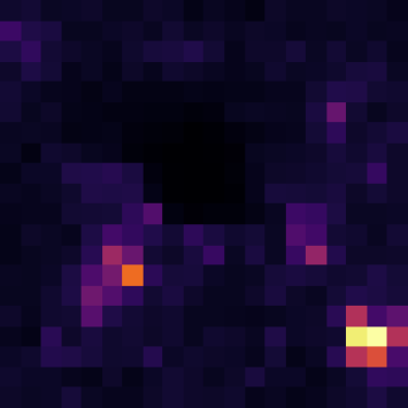
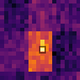
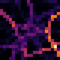
We observe that different regions hold varying importance at different time intervals, making it unnecessary to include all regions in each prediction. For example, if we know the traffic conditions on a particular highway, we can infer the traffic conditions for other regions on the same highway, thus eliminating the need to include them all. Figure 1a illustrates the traffic in the German city Hannover between am on a weekday. High traffic volumes towards the east, north-west, and south correspond to highways, while moderate to low traffic in central areas correspond to residential, commercial, and recreational areas. Figure 1b shows the corresponding attention map generated by ST-SampleNet. It can be seen that ST-SampleNet requires only a limited amount of regions of varying traffic levels (from low to high) to predict the city-wide traffic conditions indicating that other regions are redundant, i.e., their traffic can be inferred using the information from the important regions.
Therefore, we propose a lightweight region sampling strategy that prunes non-essential regions at different intervals and addresses the quadratic complexity inherent in self-attention mechanisms. For sampling, we utilised Gumbel-Softmax [15], which has a two-fold advantage. Firstly, it is differentiable, thus making end-to-end training possible. Secondly, it introduces stochasticity to the sampling process, occasionally selecting non-important regions, thereby enhancing the model’s generalisation capability through exploratory behaviour.
Additionally, we introduce a spatially constrained and learnable position embedding (SCPE) that integrates neighbourhood information in a hierarchical manner, such as locality, city, and state levels and enhances semantic interpretability. This approach constrains the self-attention mechanism to prioritise immediate neighbours, while simultaneously the learnable structure of the embedding also provides the flexibility to capture relations among distant neighbours. Consequently, SCPE not only comprehends spatial dependencies across different distances but also offers semantic interpretability.
Thus, overall, our contributions are as follows:
-
•
We propose ST-SampleNet111https://github.com/ashusao/ST-SampleNet, a novel spatio-temporal prediction model that effectively captures crucial spatio-temporal relations, including global relations, often neglected in prior approaches.
-
•
We propose a lightweight region sampling strategy that prunes the non-important regions and makes ST-SampleNet efficient.
-
•
We propose a learnable and interpretable position embedding that embeds spatial neighbourhood information.
-
•
Experiments on three real-world datasets prove the efficiency and effectiveness of ST-SampleNet.
2 Preliminaries
In this section, we formally define the problem of spatio-temporal prediction and the external features used in ST-SampleNet.
2.1 Problem Statement
Region
Following [33], we divide a city into uniform grids, each representing a distinct region denoted as , .
Spatio-Temporal Image
During each time interval , we collect spatio-temporal measurements [33] (e.g., inflow/outflow) for individual regions. The measurements for each region are combined to create a single-channel image, and multiple such images are stacked together to construct a spatio-temporal image (referred to as an image) [36], denoted as . Here, signifies the total number of distinct measurements.
Spatio-Temporal Prediction
The objective is to forecast the image at the subsequent time interval given a sequence of historical images .
2.2 External Features
Spatio-temporal measurements depend on the region’s semantic attributes (e.g., residential or commercial nature) and temporal factors. For instance, peak traffic in residential and office areas can be seen during morning and evening rush hours. Hence, we incorporate these two factors as external features in our model.
Semantic Features
To capture the semantic aspects of a region, we utilise Points of Interest (POIs). For each region , the count of POIs in specific categories (e.g. count of residential buildings) is quantified as follows:
| (1) |
where indicates that the POI with location lies within region and is the set of all POIs of type in the city. Aggregated POI counts form single-channel images for each category, stacked to create the multi-dimensional POI image , with denoting the total number of distinct categories.
Temporal Features
Regarding temporal information, we employ one-hot encoding to capture day-of-the-week information and weekend status . Due to the cyclic nature of the time of day (), sinusoidal encoding is applied:
| (2) |
where represents the time elapsed in minutes from midnight until the start of time interval . The three-time encodings are concatenated to form the feature vector , encompassing comprehensive temporal features in our model.
3 Approach
In this section, we present the ST-SampleNet approach, covering its architecture, spatially constrained position embedding, region sampling strategy, and training overview.
3.1 Architecture
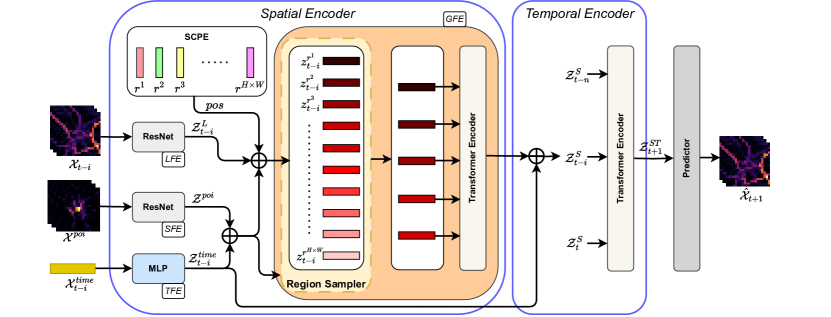
Figure 2 illustrates the architecture of ST-SampleNet. It consists of three primary components: the Spatial Encoder, the Temporal Encoder, and the Predictor. For a given timestamp , the Spatial Encoder takes three inputs: the spatio-temporal image , the semantic features of the city , and the temporal features . It processes these inputs to generate the spatial representation .
Subsequently, the Temporal Encoder operates on the spatial representations of input intervals , producing the final representation of the subsequent time interval . This final representation is then utilised by the Predictor to make predictions (). Further details regarding each component are provided below.
3.1.1 Spatial Encoder
The Spatial Encoder is responsible for capturing the spatial dependencies between regions at any time interval . It has four sub-components namely Local Feature Encoder (LFE), Semantic Feature Encoder (SFE), Temporal Feature Encoder (TFE) and Global Feature Encoder (GFE).
Local Feature Encoder (LFE)
– focuses on capturing local spatial dependencies. It utilises a ResNet [9] to achieve this. Starting with the input image , it begins with an initial convolutional layer, increasing feature dimensions to . This is followed by residual blocks designed to learn local neighbourhood relations. Each block consists of two convolutional layers and a skip connection. Finally, a convolution merges feature maps, yielding the representation of the image:
| (3) |
where . Batch Normalisation [14], and GELU [12] activation are applied after each convolution operation.
Semantic Feature Encoder (SFE)
– Regions with similar semantic attributes exhibit spatial correlations similar to traffic features often occurring in proximity. For instance, recreational amenities like bars or pubs are often clustered in city centres for convenience. Therefore, another ResNet model, similar to LFE, is employed to capture these semantic relationships and generate semantic representations:
| (4) |
The residual blocks were set to for both ResNets.
Temporal Feature Encoder (TFE)
– generates the representation for temporal features utilising a multi-layer perception (MLP) containing two linear layers with GELU activation:
| (5) |
Global Feature Encoder (GFE)
– aims to capture the global dependency amongst distant regions utilising the Transformer’s Encoder module. We first fuse all three features (, and ) along with our spatially constrained position embedding (described in Section 3.2) that provides region position information through element-wise addition. The fused representation corresponding to each region is indicated by .
Since not all regions hold equal significance at different intervals, our region sampling module (elaborated in Section 3.3) then assigns importance weights to the fused representation of each region indicated by the colour darkness in the figure. Using these weights, only the top- regions are selected and utilised by the self-attention mechanism of the Transformer Encoder [26] to learn the global relation amongst the region and generate the final spatial representation for the image at time interval :
| (6) |
3.1.2 Temporal Encoder
The Temporal Encoder captures the temporal dependency between images of different time intervals. Time is a crucial factor in determining the traffic trend; for instance, if it’s late evening, traffic generally decreases as people commute back from work and vice versa in the early morning. Therefore, we first fuse the temporal features with the spatial representation of images of input time intervals and then learn the temporal dependencies between them using another Transformer Encoder:
| (7) |
where is the spatio-temporal representation for the next time interval .
3.1.3 Predictor
The Predictor makes the final prediction utilising the spatio-temporal representation . It consists of a linear layer followed by activation:
| (8) |
where W and B are the predictor’s learnable parameters.
3.2 Spatially Constrained Position Embedding
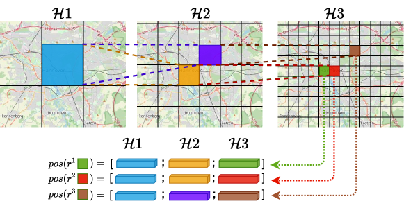
We employ a hierarchical method for embedding the position information of regions, as illustrated in Figure 3. To encode the position of a region , we embed its position at multiple levels (, , ). The lowest level captures the position at the highest granularity (e.g., ), while the highest level captures the position at the lowest granularity (e.g., ). The embeddings at different levels are concatenated to form the position embedding of the region :
| (9) |
where represents the learnable embedding dictionary at level . We set to in our model.
Semantically, SCPE captures hierarchical position information, including locality, city, state, country, etc. Crucially, it informs the self-attention mechanism about each region’s relative position, indicating proximity or distance. For example, in Figure 3, regions and are immediate neighbours at two levels ( and ), resulting in similar embedding vectors at those levels (depicted in blue and yellow). In contrast, , a distant region, exhibits similarity at only one level (depicted in blue). Consequently, this structure encourages the self-attention mechanism to prioritise attention to immediately adjacent neighbours while at the same time, its learnable design also allows it to learn the dependencies amongst distant neighbours. Thus, our SCPE not only captures spatial dependencies at varying distances but also enhances semantic interpretation.
Our proposed position embedding has important application in diverse spatio-temporal tasks, specifically, when dealing with multiple geospatial points spanning various distances, from close (e.g., ) to very distant (e.g., ) such as trajectory representation learning [16, 7], trajectory similarity comparison [27, 19] etc.
3.3 Region Sampling
The importance of a region depends on its semantic attributes and the time of day. For instance, commercial regions are crowded during working hours and deserted during non-working hours. Therefore, we utilise semantic and temporal representations to predict an importance score for each region. Specifically, we first fuse and and project them using an MLP consisting of a linear layer and GELU activation:
| (10) |
To assign importance scores and prune regions, a naive approach involves mixing the representation of all regions using an MLP to generate a score for each region. However, this method increases the parameter count by , making it inefficient. Instead, we introduce a lightweight module that applies MLP individually to each region, thereby increasing the parameter count by . To incorporate global information into the MLP, we split the sampler’s representation () of each region into two parts: the first half is denoted as local features (), where , and we compute the mean across all regions from the second half to obtain the global feature (). We concatenate the local and global features and apply the MLP to compute the probabilities to keep or drop the region:
| (11) |
where and indicate the probabilities to drop and keep a region , respectively.
Sampling directly from the distribution presents a challenge for end-to-end training due to its non-differentiability. To overcome this, we employ the Gumbel-Softmax technique [15]. This method is applied to the probability distribution of the regions to be kept, allowing us to sample important regions while ensuring the differentiability of the operation. Furthermore, Gumbel-Softmax introduces randomness to the sampling process, enabling the occasional selection of less important regions. This stochastic element enhances the model’s robustness and its ability to generalize.
3.4 Training
To avoid training being dominated by large deviations, we utilise the mean squared error (MSE) together with the mean absolute error (MAE) as the loss function, which are defined as follows:
| (12) |
| (13) |
Furthermore, we use self-distillation to mitigate the information loss from region pruning at each time interval . Our goal is to align the behaviour of the region-pruned student model with the teacher model containing all regions. It is achieved by minimizing the KL divergence [18] between their spatial representations at each input time interval :
| (14) |
where is the total number of input time intervals.
The overall training loss is the combination of the above three losses:
| (15) |
where we set in all our experiments.
4 Evaluation Setup
This section details our experiment setup, including the dataset, baseline models, and experimental settings.
4.1 Datasets
| Hannover | Dresden | NYC | |
| Latitude | |||
| Longitude | |||
| Grid size | |||
| #Regions | |||
| Time span | Jul - Dec 2019 | Jul - Dec 2019 | Jul - Dec 2023 |
| Time Interval | 1 hour | 1 hour | 1 hour |
We utilised floating car data from two German cities, Hannover and Dresden, as well as publicly available taxi data222https://www.nyc.gov/site/tlc/about/tlc-trip-record-data.page from New York City (NYC). Each city was divided into regions. For the floating car data, we computed three types of measurements (): Inflow and Outflow [33], representing the number of vehicles entering and exiting the region, respectively, and Density [17], measuring the number of vehicles within a region during a specific time interval. For NYC taxi data, we computed two types of measurements (): Pickup and DropOff [30], indicating the number of taxis picked up and dropped off in a region, respectively. Dataset details are provided in Table 1.
Additionally, we extracted categories of POIs from OpenStreetMap [21] to capture semantic characteristics. The POI categories and their counts for the three cities are described in Table 2.
| Category | Count | ||
|---|---|---|---|
| Hannover | Dresden | NYC | |
| Commercial | 1,008 | 1,618 | 752 |
| Culture | 557 | 418 | 1,100 |
| Education | 306 | 339 | 655 |
| Health | 513 | 698 | 891 |
| Public Service | 486 | 572 | 823 |
| Recreation | 1,314 | 1,256 | 7,362 |
| Residential | 6,265 | 858 | 218 |
| Sports | 882 | 923 | 1,740 |
| Tourism | 869 | 1,178 | 1,687 |
| Transport | 2,028 | 2,960 | 1,518 |
4.2 Baselines
We compare ST-SampleNet to the following baselines:
-
•
Historical Average (HA) – predicts by computing the average value of historical measurements.
-
•
DeepST [33] – utilises CNNs to process the images corresponding to closeness, period, and trend, respectively. Subsequently, it employs element-wise addition to combine all the information.
-
•
ST-ResNet [34] – updates the CNN backbone of DeepST with that of the ResNet architecture.
-
•
HConvLSTM [32] – utilises ConvLSTM layers to jointly capture the spatio-temporal dependencies by only considering the closest historical time intervals to make the prediction.
-
•
DeepSTN+ [6] – is an upgrade of ST-ResNet using a ResPlus unit that conducts two types of convolution: one to capture local neighbourhood relations with a smaller kernel size, and another to capture relations among remote regions with a larger kernel size.
-
•
BDSTN [2] – is a transformer-based architecture that first applies a multi-layer perception to learn spatial dependencies and then employs a transformer encoder to learn temporal dependencies.
-
•
ST-GSP [35] – enhances BDSTN by replacing the MLP with that of a ResNet architecture for learning spatial dependencies.
-
•
DeepCrowd [17] – stacks ConvLSTM layers in a pyramid architecture and fuses low and high-resolution feature maps to learn better feature representations.
- •
-
•
ST-3DMDDN [11] – updates ST-3DGMR by breaking the 3D Convolution into 2D Convolution in spatial dimension and 1D Convolution in temporal dimension. This significantly lowers the number of parameters and increases the model’s efficiency.
4.3 Experimental Settings
We designate December 2019 as the test set for Hannover and Dresden and December 2023 for New York. The remaining data of each city serves as the training set. To ensure model robustness, 20% of the training data is used for validation. ST-SampleNet’s feature dimension is set to 128. Following prior work [6, 34], the historical time interval’s closeness, period, and trend are set to , , and , respectively to select historical spatio-temporal images.
All models are trained on NVIDIA RTX A6000 GPUs using the AdamW optimiser [20]. The learning rate is tuned within [, , , ]. Training is conducted for epochs or until the validation error stagnates for consecutive epochs. Models achieving the best performance on the respective validation set are selected and evaluated on the test set. The effectiveness of the models is measured using root mean squared error (RMSE) and mean absolute error (MAE), whereas efficiency is measured using Giga Floating-Point Operations Per Second (GFLOPS)333We use the calflops [31] module to compute GFLOPS of our model..
5 Result
This section presents ST-SampleNet’s results, including baseline comparisons, sampling performance analysis, component contributions, spatial position embedding exploration, and a case study on sampling behaviour.
5.1 Comparison with Baselines
| Approach | Hannover | Dresden | NYC | |||||||||||||
|---|---|---|---|---|---|---|---|---|---|---|---|---|---|---|---|---|
| Density | Inflow | Outflow | Density | Inflow | Outflow | Pickup | Dropoff | |||||||||
| RMSE | MAE | RMSE | MAE | RMSE | MAE | RMSE | MAE | RMSE | MAE | RMSE | MAE | RMSE | MAE | RMSE | MAE | |
| HA | 20.22 | 11.69 | 19.61 | 11.12 | 19.66 | 11.11 | 20.39 | 10.44 | 17.92 | 9.78 | 18.03 | 9.78 | 21.04 | 4.60 | 19.07 | 4.49 |
| HConvLSTM | 9.27 | 5.54 | 9.28 | 5.50 | 9.19 | 5.43 | 9.30 | 5.29 | 9.00 | 5.16 | 8.88 | 5.10 | 8.36 | 1.67 | 6.92 | 1.49 |
| DeepST | 9.13 | 4.95 | 9.23 | 4.99 | 9.15 | 4.91 | 9.05 | 5.23 | 8.71 | 5.08 | 8.65 | 5.03 | 8.20 | 1.63 | 6.85 | 1.47 |
| ST-ResNet | 8.49 | 4.86 | 8.45 | 4.84 | 8.59 | 4.87 | 8.61 | 4.68 | 7.84 | 4.38 | 8.08 | 4.47 | 7.87 | 1.57 | 6.77 | 1.44 |
| DeepSTN+ | 8.32 | 4.46 | 8.18 | 4.45 | 8.17 | 4.42 | 8.18 | 4.13 | 7.70 | 4.05 | 7.68 | 4.01 | 7.76 | 1.45 | 6.66 | 1.34 |
| DeepCrowd | 8.29 | 4.74 | 8.23 | 4.70 | 8.21 | 4.68 | 8.04 | 4.51 | 7.67 | 4.39 | 7.61 | 4.38 | 7.66 | 1.52 | 6.57 | 1.32 |
| BDSTN | 8.08 | 4.54 | 8.05 | 4.50 | 8.01 | 4.46 | 8.11 | 4.10 | 7.67 | 4.05 | 7.70 | 4.04 | 7.50 | 1.42 | 6.25 | 1.28 |
| ST-GSP | 7.90 | 4.46 | 7.93 | 4.43 | 7.90 | 4.41 | 7.93 | 4.01 | 7.66 | 4.01 | 7.69 | 4.00 | 7.24 | 1.40 | 6.07 | 1.29 |
| ST-3DGMR | 7.76 | 4.40 | 7.81 | 4.39 | 7.78 | 4.37 | 7.93 | 4.02 | 7.63 | 3.90 | 7.64 | 3.97 | 7.37 | 1.41 | 5.91 | 1.26 |
| ST-3DMDDN | 7.62 | 4.31 | 7.72 | 4.32 | 7.67 | 4.29 | 7.75 | 3.91 | 7.59 | 3.88 | 7.60 | 3.94 | 7.03 | 1.37 | 5.84 | 1.25 |
| ST-SampleNet | 7.01 | 4.00 | 7.11 | 4.03 | 7.10 | 4.01 | 7.22 | 3.66 | 7.08 | 3.63 | 7.06 | 3.62 | 6.64 | 1.28 | 5.48 | 1.17 |
| Improv. (%) | 8.01 | 7.19 | 7.90 | 6.71 | 7.43 | 6.52 | 6.84 | 6.39 | 6.72 | 6.44 | 7.10 | 8.12 | 5.54 | 6.57 | 6.16 | 6.4 |
The performance comparison of ST-SampleNet and baselines on three datasets is detailed in Table 3. The naive historical average (HA) performs the worst, emphasising the limitations of a simple heuristic-based approach in capturing the complex spatio-temporal dynamics of a city.
Among the deep learning baselines, HConvLSTM performs the poorest due to its limited consideration of only the closest historical information, disregarding periodicity and trend information. CNN-based approaches (DeepST, ST-Resnet, and DeepSTN+) perform better than HConvLSTM but exhibit inferior performance compared to DeepCrowd, BDSTN, and ST-GSP, attributed to their negligence of capturing temporal dependencies. The recently introduced 3D Convolution-based models ST-3DGMR and ST-3DMDDN exhibit the best performance among all baselines.
ST-SampleNet outperforms the best baseline (ST-3DMDDN) by an average of w.r.t. RMSE and w.r.t. MAE across all the datasets, highlighting the importance of careful modelling all the three types of spatio-temporal relations in the architecture.
5.2 Effect of Sampling

Figure 4 depicts the effect of sampling on the performance of ST-SampleNet. The values on the x-axis indicate the ratio of the regions kept after sampling. The values on the left and right axes indicate the RMSE in the density prediction of Hannover and GLOPS taken by the model.
It can be seen that the computational cost monotonically decreases as the region keep ratio decreases except at the keep ratio of . This is due to the addition of region sampling module parameters, which is not present on the base model when full attention is applied at a keep ratio of .
Regarding performance, it can be seen that at first, the model gets better by approximately and then the performance degrades. This is because until a certain threshold ( in this case), redundant and non-essential regions are pruned, thus, there is no loss of information. Additionally, distillation from the base model further regularises the model and makes it robust. Afterwards, the loss of information becomes significant, and performance degrades. To investigate this further, we also perform a case study which is described in Section 5.5.
Overall, comparing effectiveness with efficiency, ST-SampleNet can reduce the computational cost by approximately 40% at the marginal drop in performance of around 1%.
5.3 Contribution of Different Components
In this study, we aim to investigate the contribution ST-SampleNet’s different components for which we evaluated the following variants of ST-SampleNet on the Hannover dataset:
- •
-
•
w/o LFE – In this variant, we replace ResNet of LFE with that of a linear layer similar to BERT or ViT [4].
-
•
w/o SFE – We remove the ResNet of SFE, and semantic features are not fed to the model.
-
•
w/o TFE – Temporal features are not fed to the model in this variant.
-
•
w/o GFE – We remove the transformer encoder of GFE responsible for capturing global spatial dependency.
-
•
w/o Temp. Enc. – We remove the transformer encoder responsible for capturing temporal dependency, and the mean spatial representation of input intervals is fed to the predictor.
| Volume | Inflow | Outflow | ||||
|---|---|---|---|---|---|---|
| RMSE | MAE | RMSE | MAE | RMSE | MAE | |
| ST-SampleNet | 7.01 | 4.00 | 7.11 | 4.03 | 7.10 | 4.01 |
| w/o SCPE | 7.17 | 4.07 | 7.27 | 4.09 | 7.25 | 4.07 |
| w/o LFE | 7.28 | 4.12 | 7.36 | 4.13 | 7.33 | 4.11 |
| w/o SFE | 7.16 | 4.01 | 7.29 | 4.06 | 7.24 | 4.03 |
| w/o TFE | 7.12 | 4.05 | 7.20 | 4.07 | 7.18 | 4.05 |
| w/o GFE | 7.22 | 4.10 | 7.34 | 4.13 | 7.32 | 4.11 |
| w/o Temp. Enc. | 7.28 | 4.12 | 7.38 | 4.15 | 7.38 | 4.13 |
The results in Table 4 demonstrate that each component contributes to the effectiveness of ST-SampleNet. Specifically, the contributions of LFE, GFE, and Temporal Encoder are the most important, emphasising the significance of capturing the local, global and temporal relation in spatio-temporal modelling.
5.4 Learned Position Embedding
To further investigate the impact of Spatially Constrained Position Embedding (SCPE), we compare it with a learnable position embedding akin to BERT [3] as described in Section 5.3 (w/o SCPE). Results detailed in Table 4 demonstrate that passing neighbourhood information and constraining the model to pay more attention to closed neighbours ST-SampleNet’s effectiveness.
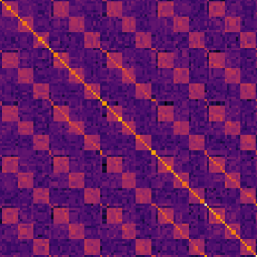
Furthermore, Figure 5 depicts the correlation of the learned position embedding, where Figure 5 depicts how each region in the Hannover city correlates to another. The small square structures along the diagonal indicate that each region primarily attends to its immediate neighbours. Given that the regions are arranged row by row in this figure, the spaces before and after these squares represent the neighbouring regions of the rows above and below, respectively. To better understand this, we also visualise the correlation of a specific region, illustrated in Figure 5b. This figure demonstrates how one region is related to the others in the city. It demonstrates the hierarchical nature where regions close to each other are more related than others.
Thus, our SCPE, offering both semantic interpretability and improved predictive capability, proves beneficial for ST-SampleNet.
5.5 Case Study: Sampling Behaviour
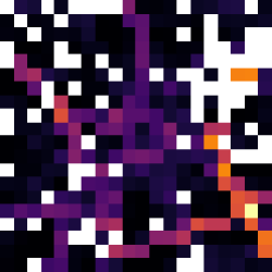

To understand the sampling behaviour of our ST-SampleNet, we performed a case study as illustrated in Figure 6. Figure 6a portrays the traffic patterns in Hannover between and am on a typical working day. Meanwhile, Figure 6b and Figure 6c exhibit the regions pruned to generate the representation of the same time interval at a keep ratio of and , respectively.
Looking at the regions pruned at a ratio of , it can be observed that ST-SampleNet prunes two types of regions. The first category comprises regions with consistently negligible traffic, such as forested areas or regions containing lakes. The second category includes regions characterised by deterministic traffic patterns, exemplified by highways in the northeast of the city. Since these regions often contain redundant information, with traffic patterns mirroring those in other parts of the city, ST-SampleNet considers them non-essential and prunes them. For instance, the traffic on pruned highways in the northeast can be accurately predicted based on the traffic of interconnected highways in the southeast and east.
However, at the keep ratio of , ST-SampleNet tends to overprune, neglecting important non-redundant regions. Notably, regions towards the city centre, where traffic exhibits significant variability due to factors such as events, weather, etc., are overlooked. Consequently, the model’s performance degrades, as discussed in Section 5.2 and illustrated in Figure 4 earlier.
6 Related Work
Spatio-temporal prediction models have gained significant attention in the realm of smart city applications, leading to the development of numerous spatio-temporal models in recent years.
Early endeavours in this domain primarily focused on capturing local spatial relations. They utilised fully convolutional architectures where spatio-temporal images of input time intervals are stacked as channels and convolutions are used to capture both spatial and temporal dependencies, such as by DeepST [33], ST-ResNet [34], and DeepSTN+ [6].
However, these approaches tend to be inefficient in modelling complex temporal dependencies inherent in spatio-temporal data, relying solely on CNNs to capture them. Consequently, subsequent works proposed a two-component approach, separating the modelling of spatio-temporal dependency into spatial and temporal aspects. Works like DMVST-Net [28] and STDN [29] pioneered this shift, utilising CNNs for spatial dependency and RNNs (LSTMs and GRUs) for temporal dependencies.
The advent of ConvLSTM [24] and ConvGRU [1] architectures further advanced spatio-temporal prediction techniques, evident in works like Periodic-CRN [36] and DeepCrowd [17]. Later, as Transformers [26] gained popularity for their superior ability to capture temporal dependency compared to LSTMs and GRUs, recent works utilised them to capture the temporal dependencies, as demonstrated by BDSTN [2] and ST-GSP [35].
More recent approaches draw inspiration from video representation learning [22], treating spatio-temporal data as sequences of frames and applying 3D Convolution to jointly learn spatio-temporal representations. Models such as ST-3DGMR [10] and ST-3DMDDN [11] exemplify this paradigm.
Unlike previous methods focusing on local neighbourhood relations via CNNs, our approach diverges by incorporating the self-attention mechanism to capture global relations. Furthermore, for efficiency, our sampling strategy mitigates the quadratic computational complexity associated with self-attention.
7 Conclusion
ST-SampleNet is a novel architecture for spatio-temporal modelling, effectively capturing essential spatio-temporal relations, including global spatial dependency often neglected in prior approaches. We propose a spatial position embedding which is semantically interpretable and enhances model performance. Additionally, our region sampling strategy in ST-SampleNet enhances efficiency by significantly reducing computation costs while maintaining performance.
This work was partially funded by the Federal Ministry for Economic Affairs and Climate Action (BMWK), Germany (“ATTENTION!”, 01MJ22012D), and by the Federal Ministry for Digital and Transport (BMDV), Germany (“MoToRes”, 19F2271A).
References
- Ballas et al. [2016] N. Ballas, L. Yao, C. Pal, and A. C. Courville. Delving deeper into convolutional networks for learning video representations. In 4th International Conference on Learning Representations, ICLR 2016, San Juan, Puerto Rico, May 2-4, 2016, Conference Track Proceedings, 2016.
- Cao et al. [2022] D. Cao, K. Zeng, J. Wang, P. K. Sharma, X. Ma, Y. Liu, and S. Zhou. Bert-based deep spatial-temporal network for taxi demand prediction. IEEE Transactions on Intelligent Transportation Systems, 2022.
- Devlin et al. [2019] J. Devlin, M.-W. Chang, K. Lee, and K. Toutanova. BERT: Pre-training of deep bidirectional transformers for language understanding. In Proceedings of the 2019 Conference of the North American Chapter of the Association for Computational Linguistics: Human Language Technologies, Volume 1 (Long and Short Papers), 2019.
- Dosovitskiy et al. [2021] A. Dosovitskiy, L. Beyer, A. Kolesnikov, D. Weissenborn, X. Zhai, T. Unterthiner, M. Dehghani, M. Minderer, G. Heigold, S. Gelly, J. Uszkoreit, and N. Houlsby. An image is worth 16x16 words: Transformers for image recognition at scale. In International Conference on Learning Representations, 2021.
- Elmi [2020] S. Elmi. Deep stacked residual neural network and bidirectional lstm for speed prediction on real-life traffic data. In Proceedings of ECAI, 2020.
- Feng et al. [2021] J. Feng, Y. Li, Z. Lin, C. Rong, F. Sun, D. Guo, and D. Jin. Context-aware spatial-temporal neural network for citywide crowd flow prediction via modeling long-range spatial dependency. ACM Trans. Knowl. Discov. Data, 2021.
- Fu and Lee [2020] T.-Y. Fu and W.-C. Lee. Trembr: Exploring road networks for trajectory representation learning. ACM Trans. Intell. Syst. Technol., 2020.
- Hameed [2019] A. A. Hameed. Smart city planning and sustainable development. IOP Conference Series: Materials Science and Engineering, may 2019.
- He et al. [2016] K. He, X. Zhang, S. Ren, and J. Sun. Deep residual learning for image recognition. In 2016 IEEE Conference on Computer Vision and Pattern Recognition (CVPR), 2016.
- He et al. [2023] R. He, Y. Xiao, X. Lu, S. Zhang, and Y. Liu. St-3dgmr: Spatio-temporal 3d grouped multiscale resnet network for region-based urban traffic flow prediction. Information Sciences, may 2023.
- He et al. [2024] R. He, C. Zhang, Y. Xiao, X. Lu, S. Zhang, and Y. Liu. Deep spatio-temporal 3d dilated dense neural network for traffic flow prediction. Expert Systems with Applications, 2024.
- Hendrycks and Gimpel [2016] D. Hendrycks and K. Gimpel. Bridging nonlinearities and stochastic regularizers with gaussian error linear units. CoRR, 2016.
- Huang et al. [2020] R. Huang, C. Huang, Y. Liu, G. Dai, and W. Kong. Lsgcn: Long short-term traffic prediction with graph convolutional networks. In Proceedings of the Twenty-Ninth International Joint Conference on Artificial Intelligence. International Joint Conferences on Artificial Intelligence Organization, 2020.
- Ioffe and Szegedy [2015] S. Ioffe and C. Szegedy. Batch normalization: Accelerating deep network training by reducing internal covariate shift. In Proceedings of the 32nd International Conference on International Conference on Machine Learning - Volume 37, 2015.
- Jang et al. [2017] E. Jang, S. Gu, and B. Poole. Categorical reparameterization with gumbel-softmax. In 5th International Conference on Learning Representations, ICLR 2017, 2017.
- Jiang et al. [2023a] J. Jiang, D. Pan, H. Ren, X. Jiang, C. Li, and J. Wang. Self-supervised trajectory representation learning with temporal regularities and travel semantics. In 2023 IEEE 39th International Conference on Data Engineering (ICDE), 2023a.
- Jiang et al. [2023b] R. Jiang, Z. Cai, Z. Wang, C. Yang, Z. Fan, Q. Chen, K. Tsubouchi, X. Song, and R. Shibasaki. Deepcrowd: A deep model for large-scale citywide crowd density and flow prediction. IEEE Transactions on Knowledge and Data Engineering, 2023b.
- Kim et al. [2021] T. Kim, J. Oh, N. Y. Kim, S. Cho, and S.-Y. Yun. Comparing kullback-leibler divergence and mean squared error loss in knowledge distillation. In Proceedings of the Thirtieth International Joint Conference on Artificial Intelligence, IJCAI-21, 2021.
- Li et al. [2018] X. Li, K. Zhao, G. Cong, C. S. Jensen, and W. Wei. Deep representation learning for trajectory similarity computation. In 2018 IEEE 34th International Conference on Data Engineering (ICDE), 2018.
- Loshchilov and Hutter [2019] I. Loshchilov and F. Hutter. Decoupled weight decay regularization. In International Conference on Learning Representations, 2019.
- OpenStreetMap contributors [2023] OpenStreetMap contributors. Planet dump retrieved from https://planet.osm.org . https://www.openstreetmap.org, 2023.
- Qian et al. [2021] R. Qian, T. Meng, B. Gong, M.-H. Yang, H. Wang, S. Belongie, and Y. Cui. Spatiotemporal contrastive video representation learning. In Proceedings of the IEEE/CVF Conference on Computer Vision and Pattern Recognition (CVPR), 2021.
- Rao et al. [2022] X. Rao, H. Wang, L. Zhang, J. Li, S. Shang, and P. Han. Fogs: First-order gradient supervision with learning-based graph for traffic flow forecasting. In Proceedings of the Thirty-First International Joint Conference on Artificial Intelligence. International Joint Conferences on Artificial Intelligence Organization, 2022.
- Shi et al. [2015] X. Shi, Z. Chen, H. Wang, D.-Y. Yeung, W.-k. Wong, and W.-c. Woo. Convolutional lstm network: A machine learning approach for precipitation nowcasting. In Proceedings of the 28th International Conference on Neural Information Processing Systems - Volume 1. MIT Press, 2015.
- Tran et al. [2015] D. Tran, L. Bourdev, R. Fergus, L. Torresani, and M. Paluri. Learning spatiotemporal features with 3d convolutional networks. In 2015 IEEE International Conference on Computer Vision (ICCV), 2015.
- Vaswani et al. [2017] A. Vaswani, N. Shazeer, N. Parmar, J. Uszkoreit, L. Jones, A. N. Gomez, L. u. Kaiser, and I. Polosukhin. Attention is all you need. In I. Guyon, U. V. Luxburg, S. Bengio, H. Wallach, R. Fergus, S. Vishwanathan, and R. Garnett, editors, Advances in Neural Information Processing Systems. Curran Associates, Inc., 2017.
- Yang et al. [2021] P. Yang, H. Wang, Y. Zhang, L. Qin, W. Zhang, and X. Lin. T3s: Effective representation learning for trajectory similarity computation. In 2021 IEEE 37th International Conference on Data Engineering (ICDE), 2021.
- Yao et al. [2018] H. Yao, F. Wu, J. Ke, X. Tang, Y. Jia, S. Lu, P. Gong, J. Ye, D. Chuxing, and Z. Li. Deep multi-view spatial-temporal network for taxi demand prediction. In Proceedings of the AAAI Conference on Artificial Intelligence. AAAI Press, 2018.
- Yao et al. [2019] H. Yao, X. Tang, H. Wei, G. Zheng, and Z. Li. Revisiting spatial-temporal similarity: A deep learning framework for traffic prediction. In Proceedings of the Thirty-Third AAAI Conference on Artificial Intelligence and Thirty-First Innovative Applications of Artificial Intelligence Conference and Ninth AAAI Symposium on Educational Advances in Artificial Intelligence. AAAI Press, 2019.
- Ye et al. [2019] J. Ye, L. Sun, B. Du, Y. Fu, X. Tong, and H. Xiong. Co-prediction of multiple transportation demands based on deep spatio-temporal neural network. In Proceedings of the 25th ACM SIGKDD International Conference on Knowledge Discovery & Data Mining, 2019.
- Ye [2023] X. Ye. calflops: a FLOPs and params calculate tool for neural networks in PyTorch framework, 2023. URL https://github.com/MrYxJ/calculate-flops.pytorch.
- Yuan et al. [2018] Z. Yuan, X. Zhou, and T. Yang. Hetero-convlstm: A deep learning approach to traffic accident prediction on heterogeneous spatio-temporal data. In Proceedings of the 24th ACM SIGKDD International Conference on Knowledge Discovery & Data Mining. Association for Computing Machinery, 2018.
- Zhang et al. [2016] J. Zhang, Y. Zheng, D. Qi, R. Li, and X. Yi. Dnn-based prediction model for spatio-temporal data. In Proceedings of the 24th ACM SIGSPATIAL International Conference on Advances in Geographic Information Systems. Association for Computing Machinery, 2016.
- Zhang et al. [2017] J. Zhang, Y. Zheng, and D. Qi. Deep spatio-temporal residual networks for citywide crowd flows prediction. In Proceedings of the Thirty-First AAAI Conference on Artificial Intelligence. AAAI Press, 2017.
- Zhao et al. [2022] L. Zhao, M. Gao, and Z. Wang. St-gsp: Spatial-temporal global semantic representation learning for urban flow prediction. In Proceedings of the Fifteenth ACM International Conference on Web Search and Data Mining. Association for Computing Machinery, 2022.
- Zonoozi et al. [2018] A. Zonoozi, J.-J. Kim, X. Li, and G. Cong. Periodic-crn: A convolutional recurrent model for crowd density prediction with recurring periodic patterns. In Proceedings of the 27th International Joint Conference on Artificial Intelligence. AAAI Press, 2018.