Renormalisation in maximally symmetric spaces and semiclassical gravity in Anti-de Sitter spacetime

Abstract

We obtain semiclassical gravity solutions in the Poincaré fundamental domain of $(3+1)$-dimensional Anti-de Sitter spacetime, PAdS₄, with a (massive or massless) Klein-Gordon field (with possibly non-trivial curvature coupling) with Dirichlet or Neumann boundary. Some results are explicitly and graphically presented for special values of the mass and curvature coupling (e.g. minimal or conformal coupling). In order to achieve this, we study in some generality how to perform the Hadamard renormalisation procedure for non-linear observables in maximally symmetric spacetimes in arbitrary dimensions, with emphasis on the stress-energy tensor. We show that, in this maximally symmetric setting, the Hadamard bi-distribution is invariant under the isometries of the spacetime, and can be seen as a ‘single-argument’ distribution depending only on the geodesic distance, which significantly simplifies the Hadamard recursion relations and renormalisation computations.

1 Introduction

Quantum field theory (QFT) in Anti-de Sitter spacetime (AdS) has gained substantial attention in the past years. This is undoubtedly in part because of its relevance in the AdS/CFT correspondence [1] and holography, but also because AdS is interesting its own right. To mention two of its important features, first, AdS is a maximally symmetric spacetime, which allows one to put abstract techniques of QFT in curved spacetimes in a computationally accessible setting. Second, AdS is interesting because it is not a globally hyperbolic spacetime, but instead a good testbed to see how techniques developed for QFT in globally hyperbolic spacetimes should be relaxed.

To mention some of the recent work, Dappiaggi and his collaborators have written a number of papers dealing with the construction of Klein-Gordon states with Robin boundary conditions in the Poincaré fundamental domain (PAdS) [2] and in the universal cover (CAdS) [3] of AdS. The case with dynamical Wentzell boundary conditions at the boundary of PAdS was studied in collaboration with one of us in [4, 5]. Dynamical boundary conditions not only appear naturally in holographic renormalisation [6], but are also central for the experimental verification of the dynamical Casimir effect [7], as explained in [8, 9, 10].

Some rigorous results in the algebraic QFT framework appear in [11]. Results on the propagation of singularities of Hadamard states that extend Radzikowski’s microlocal spectrum condition in globally hyperbolic spacetimes [12] to asymptotically AdS spacetimes appear in [13, 14]. Results from those papers allow for the construction of Hadamard states in asymptotically AdS spacetimes in [15]. (See also the thesis of Marta [16].)

The behaviour of renormalised observables in AdS has been studied extensively in the literature by Winstanley and collaborators [17, 18, 19, 20, 21, 22, 23]. The expectation value of the Klein-Gordon stress-energy tensor in CAdS_n ($n=2,\ldots 11$) is calculated in [17] with Neumann boundary conditions. The expectation value of the massless conformally coupled Klein-Gordon field squared with Robin boundary conditions at zero and finite temperature is studied in [18]. Under the same conditions, [19] deals with the stress-energy tensor, and very recently [20] studies the back-reaction corrections to AdS spacetime. The renormalised Klein-Gordon field squared with general mass and curvature coupling is studied in [21]. Expectation values for the stress-energy tensor, current and field-squared for fermions are studied in [22] and in [23] in the vacuum and in the case of finite temperature.

The work of Pitelli and collaborators has emphasised the interplay between boundary conditions and spacetime symmetries. They have studied the field squared in [24] with hybrid Dirichlet-Robin boundary conditions. [25] deals with the stress-energy tensor in PAdS₂ with Robin boundary conditions (see also [26, 27] for a study on the particle production in PAdS₂). The point is that states with generic Robin (or more general) boundary conditions are not invariant under the isometries of spacetime, unlike their Dirichlet or Neumann counterparts.

The construction of QFT in AdS is also important to understand QFT in relevant quotient spacetimes, such as the BTZ black hole in $n=3$ spacetime dimensions. Studies on semiclassical backreaction in BTZ appear in [28, 29].

In this paper, we are concerned with obtaining exact semiclassical gravity solutions in anti de-Sitter spacetime. More precisely, we shall work in the Poincaré fundamental domain of AdS in four spacetime dimensions, PAdS₄. Our interest stems from many angles. First of all, this is a natural extension to previous work by one of use finding semiclassical solutions in de Sitter spacetime [30], which are relevant to the cosmological constant problem, and to the related paper [31]. Second, our paper serves as a proof of concept that semiclassical gravity can be defined in so-called globally hyperbolic spacetimes with timelike boundaries, in the sense of Aké Hau, Flores and Sánchez [32]. These are spacetimes where boundary conditions on the timelike boundary render wave equations well posed.

We are also motivated by two further questions, which we plan to address in the future. The first one has to do with the construction of semiclassical gravity solutions in asymptotically AdS spacetimes. A natural approach is to use Fefferman-Graham expansions, starting from semiclassical gravity in AdS at the lowest order, and then perturbatively construct the solutions near the timelike boundary. The second question has to do with whether semiclassical AdS has better or worse stability properties than its classical counterpart [33, 34].

As a way to achieve our goal of obtaining semiclassical gravity solutions in AdS, we study in some generality how to perform renormalisation, via Hadamard subtraction, in maximally symmetric spacetimes for the Klein-Gordon field with arbitrary mass and curvature coupling. We pay special attention to the stress-energy tensor, as this is the key observable appearing on the ‘right-hand side’ of the semiclassical Einstein field equations. This is an addition to the literature in its own right, as it encompasses a number of situations of interest in a unified framework (see, for example, the literature cited above).

This paper is organised as follows. Section 2 first provides a review of the Klein-Gordon theory in maximally symmetric spacetimes, and then gives a particularly useful representation for the Hadamard bi-distribution in this class of spacetimes, by showing that it is invariant under the spacetime isometries, and that it is a function of (half the square of) the geodesic distance only. Sec. 3 is concerned with renormalisation in maximally symmetric spacetimes. Asymptotic expansions of the Hadamard coefficients are presented to sufficient accuracy to perform the renormalisation of the stress-energy tensor in $n=4$ spacetime dimensions. A simplified expression for the expectation value of the stress-energy tensor is given. The effects of changes in the renormalisation scale and the flat spacetime limit (as the radius of curvature tends to infinity) for the stress-energy tensor are studied. Sec. 4 then applies the previous techniques to obtain, in closed form, the vacuum expectation value of the Klein-Gordon stress-energy tensor in PAdS₄ with Dirichlet and Neumann boundary conditions. Sec. 5 then presents some semiclassical solutions in PAdS₄. Our final remarks appear in Sec. 6.

2 Quantum field theory in maximally symmetric spacetimes

This section provides an overview of maximally symmetric spacetimes with non-trivial curvature and of quantum states defined on these spacetimes. The main focus of the section is to show that the Hadamard condition for a free Klein-Gordon field adopts a particularly simple form, which makes renormalisation computationally economic. We achieve this by verifying that the Hadamard bi-distribution is invariant under the isometries of maximally symmetric spacetimes. It is clear that the simplifications that we find in this section for the Klein-Gordon field should apply to other theories defined by normally hyperbolic operators, but we do not discuss this any further and leave it as an interesting open question to address in the future.

2.1 Maximally symmetric spacetimes

Maximally symmetric spacetimes have positive, vanishing or negative constant curvature and, in $n$-dimensional spacetimes, $n(n+1)/2$ Killing vector fields generating isometries. The vanishing curvature case is Minkowski spacetime, with the Poincaré group as an isometry group. The positive curvature case is de Sitter spacetime, dS_n, with isometry group $O(1,n)$. The negative case is anti-de Sitter spacetime, AdS_n, with isometry group $O(2,n-1)$.

For maximally symmetric spacetimes, it is useful to express the curvature tensors in terms of their radius of curvature (see the discussion of Sec. 4.1 for details in the anti-de Sitter case). Setting $\rho^{2}=\ell^{2}>0$ for positive curvature and $\rho^{2}=-\ell^{2}<0$ for negative curvature, we have

$$R_{abcd} =\frac{1}{\rho^{2}}(g_{ac}g_{bd}-g_{ad}g{bc}),$$ (2.1)

$$R_{ab} =\frac{n-1}{\rho^{2}}g_{ab},$$ (2.2)

$$R =\frac{n(n-1)}{\rho^{2}}.$$ (2.3)

Maximally symmetric spacetimes solve the Einstein field equations, $R_{ab}-(1/2)Rg_{ab}+\Lambda g_{ab}=0$, with cosmological constant $\Lambda=(n-1)(n-2)/(2\rho^{2})$. More details about these spacetimes can be found in standard texts, such as [35].

2.2 Quantum fields and symmetric states

We consider for concreteness a Klein-Gordon field, whose free algebra of observables in a globally hyperbolic spacetime (with or without timelike boundary), $\mathcal{M}=(M,g_{ab})$, is denoted by $\mathscr{A}(\mathcal{M})$, and well known to be the unital, $\star$-algebra generated by fields, $\Phi(f)$, smeared against test functions $f$ ($f\in C_{0}^{\infty}(M)$ if the boundary is empty), subject to relations

1. $\Phi(\alpha f+g)=\alpha\Phi(f)+\Phi(g)$ for $\alpha\in\mathbb{C}$ (linearity),

2. $\Phi(f)^{\star}=\Phi(\overline{f})$ (hermiticity),

3. $\Phi((\Box-m^{2}-\xi R)f)=0$ (Klein-Gordon equation) and

4. $[\Phi(f),\Phi(g)]=-iE(f,g)1\!\!1$, where $E$ is the causal propagator of $\Box-m^{2}-\xi R$ and $1\!\!1$ is the algebra unit (commutation relations).

In the case of maximally symmetric spacetimes with non-trivial curvature, we focus on the case in which $\mathcal{M}$ is dS_n or AdS_n. In the Anti-de Sitter case, one must impose boundary conditions on the spacetime boundary, and in the above construction different boundary conditions correspond to different test-function spaces and different causal propagators, $E$. See [11] for some details in the Poincaré patch. While we will not dwell on details that are not central to this paper, in static spacetimes the definition of the observable algebra amounts to finding a suitable (non-unique) self-adjoint extension of a differential operator, which defines the spectral problem that is equivalent to solving the field equation, and considering test functions in an appropriate functional space.

Quantum (algebraic) states are linear maps $\omega:\mathscr{A}(\mathcal{M})\to\mathbb{C}$ that are (i) normalised, i.e. $\omega(1\!\!1)=1$, and (ii) positive, i.e. $\omega(A^{\star}A)\geq 0$ for any $A\in\mathscr{A}(\mathcal{M})$. The usual Hilbert space representation of the algebra can be obtained by means of the GNS construction, see e.g. [36, Sec. 1.3].

Here, we consider locally Hadamard quasi-free states of the Klein-Gordon field, which share the symmetries of the spacetime. It was noted in [37, 38] that the Wightman functions of symmetric states in a maximally symmetric spacetime are of the form

$$G^{+}_{\epsilon}({\rm x},{\rm x}^{\prime})=\mathcal{G}(\sigma_{\epsilon}({\rm x},{\rm x}^{\prime})),$$ (2.4)

i.e., they can be seen as (single-argument) functions of Synge’s world-function, $\sigma$, which measures half the squared geodesic distance between two points. More precisely, here $\sigma_{\epsilon}({\rm x},{\rm x}^{\prime})=\sigma({\rm x},{\rm x}^{\prime})+2i[T({\rm x})-T({\rm x}^{\prime})]\epsilon+2\epsilon^{2}$ is a regularised version of $\sigma$, , where $T$ is an arbitrary time function, which prescribes the distributional singular structure of $G_{\epsilon}$ (as $\epsilon\to 0^{+}$).

On the other hand, the Wightman function of a locally Hadamard state in a convex normal neighbourhood of spacetime takes the form

$$G^{+}_{\epsilon}({\rm x},{\rm x}^{\prime})=H_{\lambda\epsilon}({\rm x},{\rm x}^{\prime})+W({\rm x},{\rm x}^{\prime}),$$ (2.5)

where $H_{\lambda\epsilon}$ is a regularised version of the Hadamard bi-distribution, $H_{\lambda}$,

$$H_{\lambda}({\rm x},{\rm x}^{\prime}) =\frac{\alpha_{n}}{2}\left(\Theta(n-5/2)\frac{u({\rm x},{\rm x}^{\prime})}{\sigma^{n/2-1}({\rm x},{\rm x}^{\prime})}+p(n)v({\rm x},{\rm x}^{\prime})\log(\sigma({\rm x},{\rm x}^{\prime})/\lambda^{2})\right),$$ (2.6)

with

$$\alpha_{n} =\begin{cases}1/(2\pi),&\text{ if }n=2;\\ \Gamma(n/2-1)/(2\pi)^{n/2},&\text{ if }n\geq 2;\end{cases}$$ (2.7)

$$p(n) =\frac{1+(-1)^{n+1}}{2}.$$ (2.8)

In Eq. (2.6), $u$ and $v$ are symmetric, smooth coefficients that can be (at least formally) defined through the Hadamard recursion relations, subject to appropriate boundary conditions on the diagonal, see e.g. [40] for details. $\lambda$ is a fixed, arbitrary renormalisation scale. The factor of $5/2$ in the argument of the Heaviside $\Theta$ distribution in Eq. (2.6) can be taken to be any real number in the open interval $(2,3)$.

We shall now see that in maximally symmetric spacetimes, in analogy to Eq. (2.4), we have

$$H_{\lambda}({\rm x},{\rm x}^{\prime})=\mathcal{H}_{\lambda}(\sigma({\rm x},{\rm x}^{\prime})).$$ (2.9)

2.3 The Hadamard condition in maximally symmetric spacetimes

In a convex normal neighbourhood of a globally hyperbolic spacetime region, the Hadamard bi-distribution, $H_{\lambda}$, admits the following expansion

$$H_{\lambda}({\rm x},{\rm x}^{\prime}) =\frac{\alpha_{n}}{2}\left[\frac{\Theta(n-5/2)}{\sigma^{n/2-1}({\rm x},{\rm x}^{\prime})}\sum_{m=0}^{\infty}u_{m}({\rm x},{\rm x}^{\prime})\sigma^{m}({\rm x},{\rm x}^{\prime})+p(n)\left(\sum_{m=0}^{N}v_{m}({\rm x},{\rm x}^{\prime})\sigma^{m}({\rm x},{\rm x}^{\prime})+O\left(\sigma^{N+1}\right)\right)\log\left(\frac{\sigma({\rm x},{\rm x}^{\prime})}{\lambda^{2}}\right)\right],$$ (2.10)

where the order $N$ can be made arbitrarily large. The Hadamard recursion relations guarantee that, at any finite truncation of $H_{\lambda}$ of order $N$, say $H_{\lambda}^{N}$, the truncation will satisfy the Klein-Gordon equation modulo a $C^{N+1}$ term. Each coefficient in (2.10) can be written as [40]

$$u_{m}({\rm x},{\rm x}^{\prime}) =\sum_{j=0}^{J_{m}}\frac{(-1)^{j}}{j!}u_{(mj)a_{1}\ldots a_{j}}({\rm x})\sigma^{;a_{1}}({\rm x},{\rm x}^{\prime})\ldots\sigma^{;a_{j}}({\rm x},{\rm x}^{\prime})+O\left(\sigma^{(J_{m}+1)/2}({\rm x},{\rm x}^{\prime})\right),$$ (2.11a)

$$v_{l}({\rm x},{\rm x}^{\prime}) =\sum_{k=0}^{K_{l}}\frac{(-1)^{k}}{k!}v_{(lk)a_{1}\ldots a_{k}}({\rm x})\sigma^{;a_{1}}({\rm x},{\rm x}^{\prime})\ldots\sigma^{;a_{k}}({\rm x},{\rm x}^{\prime})+O\left(\sigma^{(K_{l}+1)/2}({\rm x},{\rm x}^{\prime})\right).$$ (2.11b)

In practice, the order of expansions $I_{m}$ and $J_{l}$ in Eq. (2.11) can be chosen according to convenience in the renormalisation procedure. For example, for the renormalisation of the stress-energy tensor in $n=4$ dimensions, it suffices to set $J_{0}=4$, $K_{0}=2$ and $K_{1}=0$ to obtain an expansion of $H_{\lambda}$ with an error term of order $O(\sigma^{3/2})$ that does not contribute, in the limiting procedure of renormalisation, to the stress-energy tensor. (See Eq. (3.5) below.)

In general, the coefficients $u_{(mj)a_{1}\ldots a_{j}}$ and $v_{(lk)a_{1}\ldots a_{k}}$ in Eq. 2.11 are symmetric tensors, and depend only on the local geometry of spacetime and the field equation coefficients; they are functions of the metric tensor, the curvature and their derivatives, and of $m$ and $\xi$. However, in maximally symmetric spacetimes, curvature is constant and does not depend on derivatives of the metric, cf. Eq. (2.3). Thus, the only available tensor indices for $u_{(mj)a_{1}\ldots a_{j}}$ and $v_{(lk)a_{1}\ldots a_{k}}$ are metric tensor indices. The general structure of the coefficients is hence that of symmetrised products of the metric tensor. It follows immediately that all coefficients with odd tensor rank vanish. For the coefficients with even tensor rank, we have the general structure

$$u_{(mj)a_{1}\ldots a_{j}}\sigma^{;a_{1}}\ldots\sigma^{;a_{j}} =C_{mj}g_{(a_{1}a_{2}}\ldots g_{a_{j-1}a_{j})}\sigma^{;a_{1}}\ldots\sigma^{;a_{j}}=2^{j/2}C_{mj}\sigma^{j/2},$$ (2.12)

where the $C_{mj}$ are constants, and similarly for the $v_{(lk)a_{1}\ldots a_{k}}$ coefficients with constants $D_{lk}$.

Hence, we can write Eq. (2.10) as

$$H_{\lambda}({\rm x},{\rm x}^{\prime}) =\frac{\alpha_{n}}{2}\left(\frac{\Theta(n-5/2)}{\sigma^{n/2-1}({\rm x},{\rm x}^{\prime})}\sum_{m=0}^{\infty}U_{m}\sigma^{m}({\rm x},{\rm x}^{\prime})+p(n)\left(\sum_{m=0}^{N}V_{m}\sigma^{m}({\rm x},{\rm x}^{\prime})+O\left(\sigma^{N+1}\right)\right)\log(\sigma({\rm x},{\rm x}^{\prime})/\lambda^{2})\right),$$ (2.13)

where the coefficients $U_{m}$ and $V_{m}$ are constants (i.e., spacetime independent), given by linear combinations of the $C_{rs}$ and of the $D_{rs}$ constants, respectively. Eq. (2.13) shows that the Hadamard bi-distribution is invariant under the isometries of spacetime and of the form of Eq. (2.9). The notation using capiatlised $U$ and $V$ emphasises that the $U_{m}$ and $V_{m}$ constants should not be confused with the diagonals, $u_{m}({\rm x},{\rm x})$ and $v_{m}({\rm x},{\rm x})$, of the coefficients appearing in Eq. (2.10).

2.4 The Hadamard recursion relations

The recursion relations for the coefficients $u_{k}$ and $v_{k}$ are remarkably simple. By Eq. (2.13), $u_{k}$ and $v_{k}$ can be seen as functions of the geodesic distance only. Furthermore, the van Vleck-Morette determinant in maximally symmetric spacetimes takes the form

$$\Delta=\left(\sqrt{-\frac{2\sigma}{\rho^{2}}}{\rm csch}\left(\sqrt{-\frac{2\sigma}{\rho^{2}}}\right)\right)^{n-1},$$ (2.14)

and defines also a (single-argument) function of $\sigma$. In the remaining of this section, we shall sometimes use the abuse of notation $u_{k}(\sigma)$, $u_{k}(\sigma)$ and $\Delta(\sigma)$ and denote a derivative with respect to the argument by a prime.

Imposing, as usual, that

$$(\Box_{x}-m^{2}-\xi R({\rm x}))H_{\lambda}({\rm x},{\rm x}^{\prime})+w({\rm x},{\rm x}^{\prime})=0,$$ (2.15)

where $w$ is a smooth bi-function, yields the Hadamard recursion relations, which we now analyse.

2.4.1 Spacetime dimension $n=2$

The recursion relations yield the tower of linear, non-homogeneous differetial equations

$$4(k+1)\sigma v_{k+1}^{\prime}(\sigma)+2(k+1)^{2}v_{k+1}(\sigma)-2(k+1)\sigma\frac{\Delta^{\prime}(\sigma)}{\Delta(\sigma)}v_{k+1}(\sigma)=-(\Box-m^{2}-\xi R)v_{k}(\sigma),$$ (2.16)

with the initial condition $v_{0}(\sigma)=-\Delta^{1/2}(\sigma)$. Since the cofficients of the differential equation (2.16) are analytic, one can solve Eq. (2.16) by a power series method writing

$$v_{k}=\sum_{j=0}^{\infty}v_{kj}\sigma^{j},$$ (2.17)

with constant $v_{kj}$ coefficients, and using the series expressions

$$\Delta(\sigma) =\sum_{j=0}^{\infty}\frac{2^{j+1}(1-2^{2j-1})B_{2j}}{(2n)!(-\rho)^{2j}}\sigma^{j},$$ (2.18a)

$$\frac{\Delta^{\prime}(\sigma)}{\Delta(\sigma)} =\frac{(n-1)}{2\sigma}\left(1-\sqrt{-\frac{2\sigma}{\rho^{2}}}\coth\left(\sqrt{-\frac{2\sigma}{\rho^{2}}}\right)\right)=(1-n)\sum_{j=1}^{\infty}\frac{2^{3j-1}B_{2j}}{(2j)!(-\rho)^{2j}}\sigma^{j-1}$$ (2.18b)

$$\Box\sigma^{k} =k(2k+n-2)\sigma^{k-1}-2k\frac{\Delta^{\prime}}{\Delta}\sigma^{k}=k(2k+n-2)\sigma^{k-1}+k(n-1)\sum_{j=1}^{\infty}\frac{2^{3j}B_{2j}}{(2j)!(-\rho)^{2j}}\sigma^{k+j-1},$$ (2.18c)

where $B_{j}$ is the $j$-th Bernoulli number. The recursion relations (2.16) then yield algebraic solutions for the $v_{kj}$ constants recursively in $k$.

2.4.2 Odd spacetime dimension $n\geq 3$

In this case, the recursion relations yield the tower of differential equations

$$2(2k+4-n)\sigma u_{k+1}^{\prime}(\sigma)+(k+1)(2k+4-n)u_{k+1}(\sigma)-(2k+4-n)\sigma\frac{\Delta^{\prime}(\sigma)}{\Delta(\sigma)}u_{k+1}(\sigma)=-(\Box-m^{2}-\xi R)u_{k}(\sigma)$$ (2.19)

with the initial condition $u_{0}=\Delta^{1/2}$.

Once again, the solutions can be obtained by the power series method, writing

$$u_{k}(\sigma)=\sum_{j=0}^{\infty}u_{kj}\sigma^{j},$$ (2.20)

with constant $u_{kj}$ coefficients and using the series expressions (2.18).

2.4.3 Even dimension $n\geq 4$

In this case, the recursion relations yield the tower of ordinary differential equations

$$2(2k+4-n)\sigma u_{k+1}^{\prime}(\sigma)+(k+1)(2k+4-n)u_{k+1}(\sigma)-(2k+4-n)\sigma\frac{\Delta^{\prime}(\sigma)}{\Delta(\sigma)}u_{k+1}(\sigma)=-(\Box-m^{2}-\xi R)u_{k}(\sigma)$$ (2.21)

for $k=0,n/2-3$ (if $n>4$) with the initial condition $u_{0}=\Delta^{1/2}$ (if $n\geq 4$) and

$$4(k+1)\sigma v_{k+1}^{\prime}(\sigma)+(k+1)(2k+n)v_{k+1}(\sigma)-2(k+1)\sigma\frac{\Delta^{\prime}(\sigma)}{\Delta(\sigma)}v_{k+1}(\sigma)=-(\Box-m^{2}-\xi R)v_{k}(\sigma),$$ (2.22)

with initial condition

$$4\sigma v_{0}^{\prime}(\sigma)+(n-2)v_{0}(\sigma)-2\sigma\frac{\Delta^{\prime}(\sigma)}{\Delta(\sigma)}v_{0}(\sigma)=-(\Box-m^{2}-\xi R)u_{n/2-2}(\sigma).$$ (2.23)

Once again, the solutions can be obtained by the power series method, writing

$$u_{k}(\sigma) =\sum_{j=0}^{\infty}u_{kj}\sigma^{j},$$ (2.24)

$$v_{k}(\sigma) =\sum_{j=0}^{\infty}v_{kj}\sigma^{j},$$ (2.25)

with constant $u_{kj}$ and $v_{kj}$ coefficients, with the aid of the series expressions (2.18).

3 Renormalisation in maximally symmetric spacetimes

We set the spacetime dimension as $n=4$, but it is clear how to extend the discussion to other dimensions. In this case, in a convex normal neighbourhood, the Hadamard bi-distribution (2.6) takes the form

$$H_{\lambda}({\rm x},{\rm x}^{\prime}) =\frac{1}{2(2\pi)^{2}}\left(\frac{\Delta^{1/2}({\rm x},{\rm x}^{\prime})}{\sigma({\rm x},{\rm x}^{\prime})}+v({\rm x},{\rm x}^{\prime})\log(\sigma({\rm x},{\rm x}^{\prime})/\lambda^{2})\right),$$ (3.1)

where $\Delta$ is given by Eq. (2.14). One can easily obtain from (2.14) the following expansion,

$$\Delta^{1/2} =1+\frac{\sigma}{2\rho^{2}}+\frac{19\sigma^{2}}{120\rho^{4}}+O(\sigma^{3}).$$ (3.2)

Furthermore, if a state, $\omega$, is Hadamard and invariant under the isometries of the spacetime, its Wightman function takes the local form

$$G^{+}_{\epsilon}({\rm x},{\rm x}^{\prime}) =\mathcal{G}(\sigma_{\epsilon}({\rm x},{\rm x}^{\prime}))=\frac{1}{2(2\pi)^{2}}\lim_{\epsilon\to 0^{+}}\left[\frac{1}{\sigma_{\epsilon}({\rm x},{\rm x}^{\prime})}\left(1+\frac{\sigma({\rm x},{\rm x}^{\prime})}{2\rho^{2}}+\frac{19\sigma^{2}({\rm x},{\rm x}^{\prime})}{120\rho^{4}}+O(\sigma^{3}({\rm x},{\rm x}^{\prime}))\right)\right.$$

$$+\left(V_{0}+V_{1}\sigma({\rm x},{\rm x}^{\prime})+O(\sigma^{2})\right)\log(\sigma_{\epsilon}({\rm x},{\rm x}^{\prime})/\lambda^{2})+w_{0}+w_{1}\sigma({\rm x},{\rm x}^{\prime})+O(\sigma^{2}({\rm x},{\rm x}^{\prime}))\Big{]},$$ (3.3)

where $V_{0}$ and $V_{1}$ are the state-independent constants, see Sec. 2.3 above (and Eq. (4.9) below for some explicit expressions in the negative curvature case), and $w_{0}$ and $w_{1}$ are free, state-dependent constants.

Eq. (2.13) justifies the the expansion of the singular structure of the two-point function in Eq. (3.3). In order to justify the expansion for the smooth term in Eq. (3.3), it suffices to remind oneself that the two-point function of symmetric states takes the form $G^{+}=\mathcal{G}(\sigma)$. Thus, performing a power series in $\sigma$ and subtracting $H_{\lambda}$ (cf. Eq. (2.13)) shows that the smooth part yields the Taylor series

$$G^{+}({\rm x},{\rm x}^{\prime})-H_{\lambda}({\rm x},{\rm x}^{\prime})=\sum_{i=0}^{I}w_{i}\sigma({\rm x},{\rm x}^{\prime})+O\left(\sigma^{I+1}({\rm x},{\rm x}^{\prime})\right),$$ (3.4)

with constant (i.e., spacetime independent) coefficients.

We emphasise that, if the state is not symmetric, the coefficients $w_{i}$ will be in general replaced by smooth, symmetric bi-functions that are not invariant under the spacetime isometries. However, the structure of the covariant Taylor expansion of the Hadamard bi-distribution (and hence of the singular structure of Hadamard states) is still given by Eq. (2.13).

The expectation value of the renormalised stress-energy tensor is defined as usual by a point-splitting and Hadamard subtraction prescription,

$$\omega(T_{ab}) :=\lim_{{\rm x}^{\prime}\to{\rm x}}\mathcal{T}_{ab}[G^{+}_{0}({\rm x},{\rm x}^{\prime})-H_{\lambda}({\rm x},{\rm x}^{\prime})]+\frac{1}{(2\pi)^{2}}g_{ab}[v_{1}]+\alpha_{1}m^{4}g_{ab}+\alpha_{2}m^{2}G_{ab}+\alpha_{3}I_{ab}+\alpha_{4}J_{ab},$$ (3.5a)

$$\mathcal{T}_{ab} :=(1-2\xi)g_{b}\,^{b^{\prime}}\nabla_{a}\nabla_{b^{\prime}}+\left(2\xi-\frac{1}{2}\right)g_{ab}g^{cd^{\prime}}\nabla_{c}\nabla_{d^{\prime}}-\frac{1}{2}g_{ab}m^{2}+2\xi\Big{[}-g_{a}\,^{a^{\prime}}g_{b}\,^{b^{\prime}}\nabla_{a^{\prime}}\nabla_{b^{\prime}}+g_{ab}g^{cd}\nabla_{c}\nabla_{d}+\frac{1}{2}G_{ab}\Big{]},$$ (3.5b)

$$[v_{1}] =\frac{1}{8}m^{4}+\frac{1}{4}\left(\xi-\frac{1}{6}\right)m^{2}R-\frac{1}{24}\left(\xi-\frac{1}{5}\right)\Box R+\frac{1}{8}\left(\xi-\frac{1}{6}\right)^{2}R^{2}-\frac{1}{720}R_{ab}R^{ab}+\frac{1}{720}R_{abcd}R^{abcd},$$ (3.5c)

$$I_{ab} :=2R_{;ab}-2g_{ab}\Box R+\frac{1}{2}g_{ab}R^{2}-2RR_{ab},,$$ (3.5d)

$$J_{ab} :=R_{;ab}-\frac{1}{2}g_{ab}\Box R-\Box R_{ab}+\frac{1}{2}g_{ab}R^{cd}R_{cd}-2R^{cd}R_{cadb}.$$ (3.5e)

In maximally symmetric spacetimes with $n=4$, $I_{ab}=J_{ab}=0$ [30], and one obtains the simple expression

$$\omega(T_{ab}) =\frac{1}{2(2\pi)^{2}}\left[-w_{1}+\frac{3\xi}{\rho^{2}}w_{0}-[v_{1}]\right]g_{ab}+\alpha_{1}m^{4}g_{ab}-\frac{3\alpha_{2}m^{2}}{\rho^{2}}g_{ab},$$ (3.6)

$$[v_{1}] =\frac{m^{4}}{8}+\left(\xi-\frac{1}{6}\right)\frac{3m^{2}}{\rho^{2}}+\left[18\left(\xi-\frac{1}{6}\right)^{2}-\frac{1}{60}\right]\frac{1}{\rho^{4}},$$ (3.7)

(cf. Eq. (71) in [40]). Note here that the coefficient $V_{1}$ in Eq. (3.3) is not the same as $[v_{1}]=\lim_{{\rm x}^{\prime}\to{\rm x}}v_{1}({\rm x},{\rm x}^{\prime})$.

3.1 Changes of renormalisation scale

Changes of the renormalisation scale introduce additional terms on the right-hand side of Eq. (3.6). Set a new renormalisation scale as $\mu^{-1}$. Renormalising the stress-energy tensor with respect to this new scale adds to the right-hand side of Eq. (3.6) the constant term

$$\lim_{{\rm x}^{\prime}\to{\rm x}}\mathcal{T}_{ab}(H_{\lambda}({\rm x},{\rm x}^{\prime})-H_{\mu^{-1}}({\rm x},{\rm x}^{\prime})) =-\frac{\log(\lambda^{2}\mu^{2})}{2(2\pi)^{2}}\lim_{{\rm x}^{\prime}\to{\rm x}}\mathcal{T}_{ab}v({\rm x},{\rm x}^{\prime})=-\frac{\log(\lambda^{2}\mu^{2})}{2(2\pi)^{2}}\left[-V_{1}+\frac{3\xi}{\rho^{2}}V_{0}\right].$$ (3.8)

3.2 The flat spacetime limit

It was argued in [30] that in the limit $|\rho^{2}|\to\infty$ the expression for the stress-energy tensor ought to vanish, as required by Wald’s stress-energy renormalisation axioms. Imposing this condition, we obtain

$$\lim_{|\rho^{2}|\to\infty}\omega(T_{ab})=\frac{1}{2(2\pi)^{2}}\left[\lim_{|\rho^{2}|\to\infty}\left(-w_{1}+\frac{3\xi}{\rho^{2}}w_{0}\right)-\left(\log(\lambda^{2}\mu^{2})+1\right)\frac{m^{4}}{8}\right]g_{ab}+\alpha_{1}m^{4}g_{ab}=0.$$ (3.9)

The limit of the state-dependent part in Eq. (3.9) can be read off from the Minkowski two-point function, $G^{+}_{\rm M}$, for in the limit, the two-point function $G^{+}$ must satisfy the Klein-Gordon equation in flat spacetime. We have

$$G^{+}_{\rm M}=\frac{mK_{1}\left(m\sqrt{2\sigma_{\rm M}}\right)}{(2\pi)^{2}\sqrt{2\sigma_{\rm M}}}=\frac{1}{2(2\pi)^{2}}\left[\frac{1}{\sigma_{\rm M}}+\left(\frac{m^{2}}{2}+\frac{m^{4}}{8}\sigma_{\rm M}+O(\sigma^{2}_{\rm M})\right)\log\left(\frac{m^{2}{\rm e}^{2\gamma}\sigma}{2{\rm e}}\right)-\frac{3m^{4}}{16}\sigma_{\rm M}\right]+O(\sigma_{\rm M}^{2}),$$ (3.10)

whereby we can identify $\lim_{|\rho^{2}|\to\infty}w_{0}=0$ and $\lim_{|\rho^{2}|\to\infty}w_{1}=-3m^{4}/16$.

In the massless case, the correct flat spacetime limit is satisfied. In the massive case, we obtain the relation

$$\alpha_{1}=\frac{1}{16(2\pi)^{2}}\left(\log\left(\frac{{\rm e}^{2\gamma}\lambda^{2}m^{2}}{2{\rm e}}\right)-2\right).$$ (3.11)

Finally, an expression for the expectation value of stress-energy tensor satisfying the correct flat spacetime limit is

$$\omega(T_{ab}) =\frac{1}{2(2\pi)^{2}}\left[-w_{1}+\frac{3\xi}{\rho^{2}}w_{0}\right]g_{ab}-\frac{1}{2(2\pi)^{2}}\left[3\left(\xi-\frac{1}{6}\right)\frac{m^{2}}{\rho^{2}}+\left(18\left(\xi-\frac{1}{6}\right)^{2}-\frac{1}{60}\right)\frac{1}{\rho^{4}}\right]g_{ab}+\alpha_{\mu}(\xi)\frac{m^{2}}{\rho^{2}}g_{ab},$$ (3.12)

where we have defined $\alpha_{\mu}(\xi)$ as

$$\alpha_{\mu}(\xi)=-3\alpha_{2}-\frac{\log(\lambda^{2}\mu^{2})}{2(2\pi)^{2}}\frac{3}{2}\left(\xi-\frac{1}{6}\right).$$ (3.13)

4 Quantum fields and semiclassical gravity in Anti-de Sitter spacetime

We are interested in finding solutions to the semiclassical gravity equations, cast in the form

$$G_{ab}({\rm x})+\Lambda g_{ab}({\rm x})=8\pi G_{\rm N}\omega(T_{ab}({\rm x})),$$ (4.1)

$$(\Box-m^{2}-\xi R({\rm x}))G^{+}({\rm x},{\rm x}^{\prime})=(\Box^{\prime}-m^{2}-\xi R({\rm x}^{\prime})G^{+}({\rm x},{\rm x}^{\prime})=0,$$ (4.2)

where $G^{+}$ is the Wightman function of the Klein-Gordon state $\omega$ in Anti-de Sitter spacetime. Here, the mass and curvature coupling of the field are allowed to take the values $m^{2}\geq 0$, $\xi\in\mathbb{R}$ and $\Lambda$ is a cosmological constant. We shall be focusing our attention on finding solutions in the Poincaré fundamental domain of Anti-de Sitter spacetime, PAdS₄, but some of the discussions in this section apply to PAdS_n with arbitrary $n\geq 2$.

4.1 The Poincaré fundamental domain of AdS spacetime

We begin by briefly introducing the Poincaré fundamental domain of Anti-de Sitter spacetime, PAdS_n. This spacetime can be seen as the ‘half’ of AdS_n covered by coordinates $t,x_{i}\in\mathbb{R}$ ($i=1,\ldots,n-2$) and $z\in(0,\infty)$, whereby the spacetime line element takes a form conformal to the $n$-dimensional Minkowski half-space line element,

$${\rm d}s^{2}= =\frac{\ell^{2}}{z^{2}}\left(-{\rm d}t^{2}+{\rm d}z^{2}+\sum_{i=1}^{n-2}{\rm d}x_{i}^{2}\right).$$ (4.3)

Here $\ell$ is the radius of curvature of AdS_n spacetime viewed as an embedded hyperboloid in an $(n+1)$-dimensional ambient, flat, pseudo-Riemannian manifold with metric signature $--+\ldots+$. AdS_n is a solution to the Einstein field equations with negative cosmological constant if the relation $\ell=\sqrt{-(n-1)(n-2)/(2\Lambda)}$ holds between the radius of curvature, $\ell$, and the cosmological constant, $\Lambda$.

The asymptotic timelike boundary of PAdS_n is approached as $z\to 0^{+}$, where boundary conditions must be prescribed for the matter fields defined in spacetime. We recall that the Riemann and Ricci tensors and the Ricci scalar in PAdS_d+1 take the simple form (cf. Eq. (2.3))

$$R_{abcd} =-\frac{1}{\ell^{2}}(g_{ac}g_{bd}-g_{ad}g_{bc}),$$ (4.4a)

$$R_{ab} =-\frac{n-1}{\ell^{2}}g_{ab},$$ (4.4b)

$$R =-\frac{n(n-1)}{\ell^{2}}.$$ (4.4c)

4.2 Quantum states in PAdS_n

We consider a free Klein-Gordon field propagating in PAdS_n. As mentioned above, the details of the axiomatic quantisation of the theory appear in [11], and we shall not repeat them here. The crucial point is that PAdS_n is a globally hyperbolic spacetime with timelike boundary in the sense of [32] and hence boundary conditions must be imposed together with the field equation.

For the purposes of this paper, we shall concentrate on Dirichlet and Neumann boundary conditions, as these preserve the isometries of the spacetime, see e.g. [25], and are therefore suitable for finding semiclassical Anti-de Sitter solutions.

The two-point functions of interest obey Eq. (4.2) in a parameter space constrained by the Breitenlohner-Freedman bound, which we write in terms of a parameter, $\nu$,

$$\nu:=\frac{1}{2}\sqrt{1+4\ell^{2}\left[m^{2}+\left(\xi-\frac{n-2}{4(n-1)}\right)R\right]}\geq 0.$$ (4.5)

The observation in [37], that for isometry-preserving states in maximally symmetric spacetimes the Wightman two-point function is a function of geodesic distance, allows one to obtain closed form expressions. To this end, it is convenient to define the function $u:\mathbb{R}_{0}^{+}\to\mathbb{R}^{+}$ by

$$u(\sigma)=\cosh^{2}\left(\sqrt{\sigma/(2\ell^{2})}\right),$$ (4.6)

where $\sigma=\frac{1}{2}s^{2}$ is Synge’s worldfunction (half the squared geodesic distance). We now quote results from [2].

4.2.1 Dirichlet boundary conditions

Let $\nu\in(0,\infty)$. We call the Wightman two-point function with Dirichlet boundary conditions $G^{+}_{\rm(D)}$. It satisfies Eq. (4.2) and $G^{+}_{\rm(D)}|_{z=0}=G^{+}_{\rm(D)}|_{z^{\prime}=0}=0$ and takes the form

$$G^{+}_{\rm(D)}(x,x^{\prime})=\lim_{\epsilon\to 0^{+}}\frac{\Gamma(\frac{n-2}{2})\Gamma(\frac{1}{2}+\nu)\Gamma(\frac{3}{2}+\nu)}{2^{n}\pi^{\frac{n}{2}}\Gamma(1+2\nu)\ell^{n-2}}u_{\epsilon}^{-\frac{n-1}{2}-\nu}{}_{2}F_{1}\left(\frac{n-1}{2}+\nu,\frac{1}{2}+\nu;1+2\nu;\frac{1}{u_{\epsilon}(x,x^{\prime})}\right),$$ (4.7)

where $u_{\epsilon}$ is defined in terms of the regularised version of Synge’s world function as $u_{\epsilon}=\cosh^{2}\left(\sqrt{\sigma_{\epsilon}/(2\ell^{2})}\right)$.

4.2.2 Neumann boundary conditions

Let $\nu\in(0,1)$. We call the Wightman two-point function with Neumann boundary conditions $G^{+}_{\rm(N)}$. It satisfies Eq. (4.2) and $\partial_{z}G^{+}_{\rm(N)}|_{z=0}=\partial_{z^{\prime}}G^{+}_{\rm(N)}|_{z^{\prime}=0}=0$ and takes the form

$$G^{+}_{\rm(N)}(x,x^{\prime})=\lim_{\epsilon\to 0^{+}}\frac{\Gamma(\frac{n-2}{2})\Gamma(\frac{1}{2}-\nu)\Gamma(\frac{3}{2}-\nu)}{2^{n}\pi^{\frac{n}{2}}\Gamma(1-2\nu)\ell^{n-2}}u_{\epsilon}^{-\frac{n-1}{2}+\nu}{}_{2}F_{1}\left(\frac{n-1}{2}-\nu,\frac{1}{2}-\nu;1-2\nu;\frac{1}{u_{\epsilon}(x,x^{\prime})}\right).$$ (4.8)

4.3 The stress-energy tensor with Dirichlet and Neumann boundary conditions

We henceforth focus on the case $n=4$, with Breitenlohner-Freedman bound $\nu=\sqrt{9/4+\ell^{2}m^{2}-12\xi}\geq 0$. We give some details for the Dirichlet case. The Neumann case can be obtained by sending $\nu$ to its negative value. For the Dirichlet case, we have the covariant Taylor series

$$G^{+}_{\rm(D)}=\frac{1}{2(2\pi)^{2}}\left\{\frac{1}{\sigma}\left(1-\frac{\sigma}{2\ell^{2}}+\frac{19\sigma^{2}}{120\ell^{4}}+O(\sigma^{3})\right)\right.$$

$$+\left[\frac{m^{2}}{2}+\frac{1}{\ell^{2}}\left(1-6\xi\right)+\frac{1}{4\ell^{2}}\left(\ell^{2}m^{2}-12\xi+2\right)\left(\frac{m^{2}}{2}-\frac{6\xi}{\ell^{2}}\right)\sigma+O(\sigma^{2})\right]\log\left(\frac{\sigma}{2\ell^{2}}\right)$$

$$+\left.\frac{2\left(4\nu^{2}-1\right)H_{\nu-\frac{1}{2}}-4\nu^{2}-\frac{1}{3}}{8\ell^{2}}+\frac{\left(4\left(4\nu^{2}-9\right)\left(4\nu^{2}-1\right)H_{\nu-\frac{1}{2}}-80\nu^{4}+\frac{280}{3}\nu^{2}+\frac{47}{5}\right)\sigma}{256\ell^{4}}+O(\sigma^{2})\right\},$$ (4.9)

where $H_{\nu-1/2}=\psi(\nu+1/2)+\gamma$ is the analytic continuation of the harmonic number function, in terms of the digamma function, $\psi$. We can read off immediately

$$w_{0} =\frac{2\left(4\nu^{2}-1\right)H_{\nu-\frac{1}{2}}-4\nu^{2}-\frac{1}{3}}{8\ell^{2}},$$ (4.10)

$$w_{1} =\frac{\left(4\left(4\nu^{2}-9\right)\left(4\nu^{2}-1\right)H_{\nu-\frac{1}{2}}-80\nu^{4}+\frac{280}{3}\nu^{2}+\frac{47}{5}\right)}{256\ell^{4}}.$$ (4.11)

Using the results of Sec. 3, we obtain, cf. Eq. (3.6)

$$\omega_{\rm(D)}(T_{ab}) =-\frac{1}{2(2\pi)^{2}}\left[\frac{\left(4\left(4\nu^{2}-9\right)\left(4\nu^{2}-1\right)H_{\nu-\frac{1}{2}}-80\nu^{4}+\frac{280}{3}\nu^{2}+\frac{47}{5}\right)}{256\ell^{4}}\right.$$

$$\left.+\frac{3\xi\left[2\left(4\nu^{2}-1\right)H_{\nu-\frac{1}{2}}-4\nu^{2}-\frac{1}{3}\right]}{8\ell^{4}}+\frac{m^{4}}{8}-\left(\xi-\frac{1}{6}\right)\frac{3m^{2}}{\ell^{2}}+\left(18\left(\xi-\frac{1}{6}\right)^{2}-\frac{1}{60}\right)\frac{1}{\ell^{4}}\right]g_{ab}$$

$$+\alpha_{1}m^{4}g_{ab}+\frac{3\alpha_{2}m^{2}}{\ell^{2}}g_{ab},$$ (4.12)

for the expectation value of the renormalised stress-energy tensor with Dirichlet boundary contions. A choice of the renormalisation constants with the correct flat-spacetime limit gives, cf. Eq. (3.12),

$$\omega_{\rm(D)}(T_{ab}) =-\frac{1}{2(2\pi)^{2}}\left[\frac{\left(4\left(4\nu^{2}-9\right)\left(4\nu^{2}-1\right)H_{\nu-\frac{1}{2}}-80\nu^{4}+\frac{280}{3}\nu^{2}+\frac{47}{5}\right)}{256\ell^{4}}\right.$$

$$\left.+\frac{3\xi\left[2\left(4\nu^{2}-1\right)H_{\nu-\frac{1}{2}}-4\nu^{2}-\frac{1}{3}\right]}{8\ell^{4}}\right]g_{ab}-\frac{1}{2(2\pi)^{2}}\left[-3\left(\xi-\frac{1}{6}\right)\frac{m^{2}}{\ell^{2}}+\left(18\left(\xi-\frac{1}{6}\right)^{2}-\frac{1}{60}\right)\frac{1}{\ell^{4}}\right]g_{ab}$$

$$-\alpha_{\mu}(\xi)\frac{m^{2}}{\ell^{2}}g_{ab}.$$ (4.13)

By a verbatim repeat, we obtain for Neumann boundary conditions

$$\omega_{\rm(N)}(T_{ab}) =-\frac{1}{2(2\pi)^{2}}\left[\frac{\left(4\left(4\nu^{2}-9\right)\left(4\nu^{2}-1\right)H_{-\nu-\frac{1}{2}}-80\nu^{4}+\frac{280}{3}\nu^{2}+\frac{47}{5}\right)}{256\ell^{4}}\right.$$

$$\left.+\frac{3\xi\left[2\left(4\nu^{2}-1\right)H_{-\nu-\frac{1}{2}}-4\nu^{2}-\frac{1}{3}\right]}{8\ell^{4}}+\frac{m^{4}}{8}-\left(\xi-\frac{1}{6}\right)\frac{3m^{2}}{\ell^{2}}+\left(18\left(\xi-\frac{1}{6}\right)^{2}-\frac{1}{60}\right)\frac{1}{\ell^{4}}\right]g_{ab}$$

$$+\alpha_{1}m^{4}g_{ab}+\frac{3\alpha_{2}m^{2}}{\ell^{2}}g_{ab}.$$ (4.14)

A choice of the renormalisation constants with the correct flat-spacetime limit gives, in the Neumann case,

$$\omega_{\rm(N)}(T_{ab}) =-\frac{1}{2(2\pi)^{2}}\left[\frac{\left(4\left(4\nu^{2}-9\right)\left(4\nu^{2}-1\right)H_{-\nu-\frac{1}{2}}-80\nu^{4}+\frac{280}{3}\nu^{2}+\frac{47}{5}\right)}{256\ell^{4}}\right.$$

$$\left.+\frac{3\xi\left[2\left(4\nu^{2}-1\right)H_{-\nu-\frac{1}{2}}-4\nu^{2}-\frac{1}{3}\right]}{8\ell^{4}}\right]g_{ab}-\frac{1}{2(2\pi)^{2}}\left[-3\left(\xi-\frac{1}{6}\right)\frac{m^{2}}{\ell^{2}}+\left(18\left(\xi-\frac{1}{6}\right)^{2}-\frac{1}{60}\right)\frac{1}{\ell^{4}}\right]g_{ab}$$

$$-\alpha_{\mu}(\xi)\frac{m^{2}}{\ell^{2}}g_{ab}.$$ (4.15)

5 Semiclassical gravity in PAdS₄

We present some solutions to the equations

$$\frac{3}{\ell^{2}}+\Lambda =8\pi G_{\rm N}\omega_{\rm(D/N)}(T_{ab})$$ (5.1)

in PAdS₄ with Dirichlet and Neumann boundary conditions. The solution space is characterised by the parameters of the theory, as the equations (5.1) reduce to an algebraic relations due to the symmetries of the spacetime, as was observed in the de Sitter case [30, 31].

If one does not demand that $\ell^{2}=-3/\Lambda$ a priori, and keeps things as general as possible [31], one needs not impose the flat spacetime limit of Sec. 3.2. We therefore use Eq. (4.12)/(4.14) for the right-hand side of Eq. (5.1).

5.1 Dirichlet boundary conditions

The solutions to Eq. (5.1) with Dirichlet boundary conditions are the solutions to the algebraic equation

$$\frac{1}{8\pi G_{\rm N}}\left(\frac{3}{\ell^{2}}+\Lambda\right)-\alpha_{1}m^{4}-\frac{3\alpha_{2}m^{2}}{\ell^{2}}$$

$$=-\frac{1}{2(2\pi)^{2}}\left[\frac{\left(4\left(4\nu^{2}-9\right)\left(4\nu^{2}-1\right)H_{\nu-\frac{1}{2}}-80\nu^{4}+\frac{280}{3}\nu^{2}+\frac{47}{5}\right)}{256\ell^{4}}\right.$$

$$\left.+\frac{3\xi\left[2\left(4\nu^{2}-1\right)H_{\nu-\frac{1}{2}}-4\nu^{2}-\frac{1}{3}\right]}{8\ell^{4}}+\frac{m^{4}}{8}-\left(\xi-\frac{1}{6}\right)\frac{3m^{2}}{\ell^{2}}+\left[18\left(\xi-\frac{1}{6}\right)^{2}-\frac{1}{60}\right]\frac{1}{\ell^{4}}\right].$$ (5.2)

Each solution is a point in the space of parameters $(\Lambda,\ell,m^{2},\xi,\alpha_{1},\alpha_{2})$, with positive $\ell$, non-negative $m^{2}$,

$$-\infty<\xi\leq\frac{4\ell^{2}m^{2}+9}{48},$$ (5.3)

and real $\Lambda$, $\alpha_{1}$ and $\alpha_{2}$.

Absorbing the parameters $\alpha_{1}$ and $\alpha_{2}$ into $\Lambda$ and the definition of $G_{\rm N}$, we can reduce the space of parameters to $(\Lambda,\ell,m^{2},\xi)$. This means that the space of solutions is a subset of $\mathbb{R}^{4}$; for every admissible $m^{2}\geq 0$, $\xi$ obeying (5.3), $\ell>0$, one can find a $\Lambda$ by imposing Eq. (5.2).

Since there are a priori no physical reasons to constraint the parameters beyond the ranges that we have given, we proceed to study a few distinguished cases. Namely, the massless, and massive minimally coupled scenarios and the ‘effectively massless’ case, which includes the conformal coupling case. (The terminology for this last case is explained in Sec. 5.1.3.)

5.1.1 The massless minimally coupled field

In this case, $m^{2}=\xi=0$ and $\nu=3/2$. Each point along the solid curve of Fig. 1 represents a solution. The equations (5.2) simplify to

$$\Lambda=-\frac{3}{\ell^{2}}+\frac{29G_{\rm N}}{120\pi\ell^{4}}$$ (5.4)

It is easy to see that $\Lambda$ attains a minimum value when $\ell=\sqrt{29G_{\rm N}/180}$, for which $\Lambda=-270\pi/(29G_{\rm N})$. As $\ell\to 0^{+}$, $\Lambda\to\infty$, and as $\ell\to\infty$, $\Lambda\to 0$, see Fig. 1,

Figure 1: The solid curve represents semiclassical PAdS₄ solutions with a massless and minimally coupled field with Dirichlet boundary conditions. The dashed curve represent semiclassical PAdS₄ solutions with a massless and minimally coupled field with Dirichlet or Neumann boundary conditions.

5.1.2 The massive minimally coupled field

In this case, $m^{2}>0$, $\xi=0$ and $\nu=\sqrt{9/4+\ell^{2}m^{2}}$. The semiclassical equations do not have a simple closed form, but we sample numerically the space of solutions. Each point in the 3-dimensional plot of Fig. 2 represents a solution.

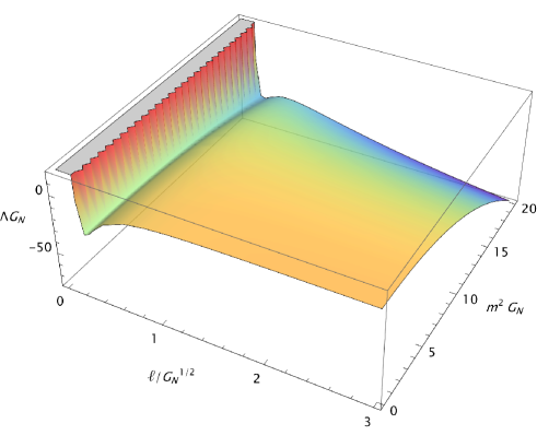
Figure 2: Semiclassical PAdS₄ solutions with a massive and minimally coupled field with Dirichlet boundary conditions.

5.1.3 Effectively massless field

For the value $\nu=1/2$, the Klein-Gordon equation in PAdS_n takes the form of a massless Klein-Gordon equation in the Minkowski half-space. For $n=4$, this occurs when $\xi=(\ell^{2}m^{2}+2)/12$. The semiclassical gravity equations simplify to

$$\Lambda=-\frac{3}{l^{2}}-\frac{G_{\rm N}}{120\pi l^{4}}$$ (5.5)

It is straightforward to see that $\Lambda$, when viewed as a function of $\ell$, is a monotonically increasing, negative function. As $\ell\to 0^{+}$, $\Lambda\to-\infty$, and as $\ell\to\infty$, $\Lambda\to 0$. The case $m^{2}=0$, $\xi=1/6$ gives solutions for a conformal field with Dirichlet boundary conditions in PAdS₄. The solutions are displayed along the dashed curve of Fig. 1.

5.2 Neumann boundary conditions

The solutions to Eq. (5.1) with Neumann boundary conditions are the solutions to the algebraic equation

$$\frac{1}{8\pi G_{\rm N}}\left(\frac{3}{\ell^{2}}+\Lambda\right)-\alpha_{1}m^{4}-\frac{3\alpha_{2}m^{2}}{\ell^{2}}$$

$$=-\frac{1}{2(2\pi)^{2}}\left[\frac{\left(4\left(4\nu^{2}-9\right)\left(4\nu^{2}-1\right)H_{-\nu-\frac{1}{2}}-80\nu^{4}+72\nu^{2}+\frac{64}{3}m^{2}\ell^{2}-256\xi+\frac{281}{3}\right)}{256\ell^{4}}\right.$$

$$\left.+\frac{3\xi\left[2\left(4\nu^{2}-1\right)H_{-\nu-\frac{1}{2}}-4\nu^{2}-\frac{1}{3}\right]}{8\ell^{4}}+\frac{m^{4}}{8}-\left(\xi-\frac{1}{6}\right)\frac{3m^{2}}{\ell^{2}}+\left[18\left(\xi-\frac{1}{6}\right)^{2}-\frac{1}{60}\right]\frac{1}{\ell^{4}}\right],$$ (5.6)

which are points in the space of parameters $(\Lambda,\ell,m^{2},\xi)$, with $\Lambda\in\mathbb{R}$ $\ell>0$, $m^{2}\geq 0$ and

$$\frac{4\ell^{2}m^{2}+5}{48}<\xi<\frac{4\ell^{2}m^{2}+9}{48}.$$ (5.7)

Note that, in view of (5.7), Neumann boundary conditions do not admit solutions with minimal coupling. In the case of the effectively massless field, the Dirichlet and Neumann boundary conditions yield the same spacetime geometry, see Fig. 1. This includes the case $m^{2}=0$, $\xi=1/6$, which represents a conformal field with Neumann boundary conditions in PAdS₄.

6 Final remarks

This paper has dealt with the question of constructing semiclassical gravity exact solutions in Anti-de Sitter spacetime. We have focused our attention in particular to PAdS₄ with a Klein-Gordon field in the vacuum obeying Dirichlet or Neumann boundary conditions. Under a suitable re-definition of parameters, the solutions are characterised by a four-dimensional parameter space, including the mass term, $m^{2}$, curvature coupling, $\xi$, AdS radius, $\ell$, and the cosmological constant, $\Lambda$.

We present some solutions for the minimally coupled case and the ‘effectively massless’ case, which includes the conformal field. These solutions are points in the plots of Sec. 5, which depict (2- and 3-dimensional) sections of the space of solutions (as subsets of the parameter space).

In this paper we have also given details on how to perform the renormalisation of non-linear observables in maximally symmetric spacetimes à la Hadamard in a computationally efficient way. The method relies on noting that the Hadamard bi-distribution shares the spacetime symmetries and takes a simplified form. This makes the computation of the Hadamard coefficients efficient and encompasses a number of situations that have been of interest in recent literature, as discussed in the Introduction.

References

- [1] J. M. Maldacena, “The Large N limit of superconformal field theories and supergravity”, Adv. Theor. Math. Phys. 2 (1998), 231-252 doi:10.4310/ATMP.1998.v2.n2.a1 [arXiv:hep-th/9711200 [hep-th]].
- [2] C. Dappiaggi and H. R. C. Ferreira, “Hadamard states for a scalar field in anti–de Sitter spacetime with arbitrary boundary conditions”, Phys. Rev. D 94 (2016) no.12, 125016 doi:10.1103/PhysRevD.94.125016 [arXiv:1610.01049 [gr-qc]].
- [3] C. Dappiaggi, H. Ferreira and A. Marta, “Ground states of a Klein-Gordon field with Robin boundary conditions in global anti–de Sitter spacetime”, Phys. Rev. D 98 (2018) no.2, 025005 doi:10.1103/PhysRevD.98.025005 [arXiv:1805.03135 [hep-th]].
- [4] C. Dappiaggi, H. R. C. Ferreira and B. A. Juárez-Aubry, “Mode solutions for a Klein-Gordon field in anti–de Sitter spacetime with dynamical boundary conditions of Wentzell type”, Phys. Rev. D 97 (2018) no.8, 085022 doi:10.1103/PhysRevD.97.085022 [arXiv:1802.00283 [hep-th]].
- [5] C. Dappiaggi, B. A. Juárez-Aubry and A. Marta, “Ground state for the Klein-Gordon field in anti–de Sitter spacetime with dynamical Wentzell boundary conditions”, Phys. Rev. D 105 (2022) no.10, 105017 doi:10.1103/PhysRevD.105.105017 [arXiv:2203.04811 [hep-th]].
- [6] K. Skenderis, “Lecture notes on holographic renormalization”, Class. Quant. Grav. 19 (2002), 5849-5876 doi:10.1088/0264-9381/19/22/306 [arXiv:hep-th/0209067 [hep-th]].
- [7] C. M. Wilson, G. Johansson, A. Pourkabirian, M. Simoen, J. R. Johansson, T. Duty, F. Nori and P. Delsing, “Observation of the dynamical Casimir effect in a superconducting circuit”, Nature 479 (2011), 376-379 doi:10.1038/nature10561
- [8] B. A. Juárez-Aubry and R. Weder, “A short review of the Casimir effect with emphasis on dynamical boundary conditions”, Supl. Rev. Mex. Fís. 3 (2022) 020714 doi:10.31349/SuplRevMexFis.3.020714 [arXiv:2112.06824 [hep-th]].
- [9] B. A. Juárez-Aubry and R. Weder, “Quantum field theory with dynamical boundary conditions and the Casimir effect”, in Theoretical physics, wavelets, analysis, genomics: An indisciplinary tribute to Alex Grossmann, Eds. P. Flandrin, S. Jaffard, T. Paul and B. Torresani (Birkhäuser, 2023) doi:10.1007/978-3-030-45847-8_12 [arXiv:2004.05646 [hep-th]].
- [10] B. A. Juárez-Aubry and R. Weder, “Quantum field theory with dynamical boundary conditions and the Casimir effect: coherent states”, J. Phys. A 54 (2021) no.10, 105203 doi:10.1088/1751-8121/abdccf [arXiv:2008.02842 [hep-th]].
- [11] C. Dappiaggi and H. R. C. Ferreira, “On the algebraic quantization of a massive scalar field in anti-de-Sitter spacetime”, Rev. Math. Phys. 30 (2017) no.2, 1850004 doi:10.1142/S0129055X18500046 [arXiv:1701.07215 [math-ph]].
- [12] M. J. Radzikowski, “Micro-local approach to the Hadamard condition in quantum field theory on curved space-time”, Commun. Math. Phys. 179 (1996), 529-553 doi:10.1007/BF02100096
- [13] O. Gannot and M. Wrochna, “Propagation of singularities on AdS spacetimes for general boundary conditions and the holographic Hadamard condition”, J. Inst. Math. Jussieu 21 (2022) no.1, 67-127 doi:10.1017/S147474802000002X [arXiv:1812.06564 [math.AP]].
- [14] C. Dappiaggi and A. Marta, “A generalization of the propagation of singularities theorem on asymptotically anti-de Sitter spacetimes”, Math. Nachr. 295 (2022) no.10, 1934-1968 doi:10.1002/mana.202000287 [arXiv:2006.00560 [math-ph]].
- [15] C. Dappiaggi and A. Marta, “Fundamental solutions and Hadamard states for a scalar field with arbitrary boundary conditions on an asymptotically AdS spacetimes”, Math. Phys. Anal. Geom. 24 (2021) no.3, 28 doi:10.1007/s11040-021-09402-5 [arXiv:2101.10290 [math-ph]].
- [16] A. Marta, A propagation of singularities theorem and a well-posedness result for the Klein-Gordon equation on asymptotically Anti-de Sitter spacetimes with general boundary conditions, PhD thesis, Universitá degli Studi di Milano, 2022.
- [17] C. Kent and E. Winstanley, “Hadamard renormalized scalar field theory on anti-de Sitter spacetime”, Phys. Rev. D 91 (2015) no.4, 044044 doi:10.1103/PhysRevD.91.044044 [arXiv:1408.6738 [gr-qc]].
- [18] T. Morley, P. Taylor and E. Winstanley, “Quantum field theory on global anti-de Sitter space-time with Robin boundary conditions”, Class. Quant. Grav. 38 (2021) no.3, 035009 doi:10.1088/1361-6382/aba58a [arXiv:2004.02704 [gr-qc]].
- [19] T. Morley, S. Namasivayam and E. Winstanley, “Renormalized stress-energy tensor on global anti-de Sitter space-time with Robin boundary conditions”, Gen. Rel. Grav. 56 (2024) no.4, 38 doi:10.1007/s10714-024-03224-w [arXiv:2308.05623 [hep-th]].
- [20] J. C. Thompson and E. Winstanley, “Quantum-corrected anti-de Sitter space-time”, [arXiv:2405.20422 [hep-th]].
- [21] S. Namasivayam and E. Winstanley, “Vacuum polarization on three-dimensional anti-de Sitter space-time with Robin boundary conditions”, Gen. Rel. Grav. 55 (2023) no.1, 13 doi:10.1007/s10714-022-03056-6 [arXiv:2209.01133 [hep-th]].
- [22] V. E. Ambrus and E. Winstanley, “Renormalised fermion vacuum expectation values on anti-de Sitter space–time”, Phys. Lett. B 749 (2015), 597-602 doi:10.1016/j.physletb.2015.08.045 [arXiv:1505.04962 [hep-th]].
- [23] V. E. Ambrus and E. Winstanley, “Thermal expectation values of fermions on anti-de Sitter space-time”, Class. Quant. Grav. 34 (2017) no.14, 145010 doi:10.1088/1361-6382/aa7863 [arXiv:1704.00614 [hep-th]].
- [24] V. S. Barroso and J. P. M. Pitelli, “Boundary conditions and vacuum fluctuations in ”, Gen. Rel. Grav. 52 (2020) no.3, 29 doi:10.1007/s10714-020-02672-4 [arXiv:1904.10920 [gr-qc]].
- [25] J. P. M. Pitelli, V. S. Barroso and R. A. Mosna, “Boundary conditions and renormalized stress-energy tensor on a Poincaré patch of AdS2”, Phys. Rev. D 99 (2019) no.12, 125008 doi:10.1103/PhysRevD.99.125008 [arXiv:1904.10806 [gr-qc]].
- [26] J. P. M. Pitelli and V. S. Barroso, “Particle production between isometric frames on a Poincaré patch of AdS2”, J. Math. Phys. 60 (2019) no.9, 092301 doi:10.1063/1.5117832 [arXiv:1908.11742 [gr-qc]].
- [27] J. P. M. Pitelli, B. S. Felipe and R. A. Mosna, “Unruh-DeWitt detector in AdS2”, Phys. Rev. D 104 (2021) no.4, 045008 doi:10.1103/PhysRevD.104.045008 [arXiv:2108.10192 [gr-qc]].
- [28] M. Casals, A. Fabbri, C. Martínez and J. Zanelli, “Quantum Backreaction on Three-Dimensional Black Holes and Naked Singularities”, Phys. Rev. Lett. 118 (2017) no.13, 131102 doi:10.1103/PhysRevLett.118.131102 [arXiv:1608.05366 [gr-qc]].
- [29] O. Baake and J. Zanelli, “Quantum backreaction for overspinning BTZ geometries”, Phys. Rev. D 107 (2023) no.8, 084015 doi:10.1103/PhysRevD.107.084015 [arXiv:2301.04256 [hep-th]].
- [30] B. A. Juárez-Aubry, “Semi-classical gravity in de Sitter spacetime and the cosmological constant”, Phys. Lett. B 797 (2019), 134912 doi:10.1016/j.physletb.2019.134912 [arXiv:1903.03924 [gr-qc]].
- [31] H. Gottschalk, N. R. Rothe and D. Siemssen, “Cosmological de Sitter Solutions of the Semiclassical Einstein Equation”, Ann. Henri Poincaré 24 (2023) no.9, 2949-3029 doi:10.1007/s00023-023-01315-z [arXiv:2206.07774 [gr-qc]].
- [32] L. Aké Hau, J. L. Flores and M. Sánchez, “Structure of globally hyperbolic spacetimes-with-timelike-boundary”, Rev. Mat. Iberoam. 37 (2021), no.1, 45 doi:10.4171/RMI/1201 [arXiv:1808.04412 [gr-qc]].
- [33] P. Bizón and A. Rostworowski, “On weakly turbulent instability of anti-de Sitter space”, Phys. Rev. Lett. 107 (2011), 031102 doi:10.1103/PhysRevLett.107.031102 [arXiv:1104.3702 [gr-qc]].
- [34] P. Bizoń, M. Maliborski and A. Rostworowski, “Resonant Dynamics and the Instability of Anti–de Sitter Spacetime”, Phys. Rev. Lett. 115 (2015) no.8, 081103 doi:10.1103/PhysRevLett.115.081103 [arXiv:1506.03519 [gr-qc]].
- [35] S. W. Hawking and G. F. R. Ellis, The Large Scale Structure of Space-Time (Cambridge University Press, 2023) doi:10.1017/9781009253161.
- [36] I. Khavkine and V. Moretti, “Algebraic QFT in curved spacetime and quasifree Hadamard states: an introduction”, in Advances in algebraic quantum field theory, Eds. R. Brunetti, C. Dappiaggi, K. Fredenhagen and J. Yngvason (Springer, 2015) doi:10.1007/978-3-319-21353-8_5 [arXiv:1412.5945 [math-ph]].
- [37] B. Allen, “Vacuum States in de Sitter Space”, Phys. Rev. D 32 (1985), 3136 doi:10.1103/PhysRevD.32.3136
- [38] B. Allen and T. Jacobson, “Vector Two Point Functions in Maximally Symmetric Spaces,” Commun. Math. Phys. 103 (1986), 669 doi:10.1007/BF01211169
- [39] C. Kent, Quantum scalar field theory on anti-de Sitter space, PhD thesis, University of Sheffield, 2013.
- [40] Y. Decanini and A. Folacci, “Hadamard renormalization of the stress-energy tensor for a quantized scalar field in a general spacetime of arbitrary dimension”, Phys. Rev. D 78 (2008), 044025 doi:10.1103/PhysRevD.78.044025 [arXiv:gr-qc/0512118 [gr-qc]].