Test-Time Training with Quantum Auto-Encoder: From Distribution Shift to Noisy Quantum Circuits
Abstract
In this paper, we propose test-time training with the quantum auto-encoder (QTTT). QTTT adapts to (1) data distribution shifts between training and testing data and (2) quantum circuit error by minimizing the self-supervised loss of the quantum auto-encoder. Empirically, we show that QTTT is robust against data distribution shifts and effective in mitigating random unitary noise in the quantum circuits during the inference. Additionally, we establish the theoretical performance guarantee of the QTTT architecture. Our novel framework presents a significant advancement in developing quantum neural networks for future real-world applications and functions as a plug-and-play extension for quantum machine learning models.
1 Introduction
Quantum computing offers an alternative approach to computation from classical computers, grounded in quantum mechanics principles such as superposition, entanglement, and interference, with the potential for reshaping the future of computing (Herrmann et al.,, 2022; Shor,, 1997). In the noisy intermediate-scale quantum (NISQ) era, quantum machine learning (QML), as an important component of variational quantum algorithms (VQAs), offers a fruitful playground for exploring theoretical aspects such as expressive power (Wen et al.,, 2024), generalization (Abbas et al.,, 2021; Huang et al.,, 2021), and overparameterization (Larocca et al.,, 2023). Additionally, it drives methodological innovation by leveraging quantum mechanical principles for learning quantum data and error correction scheme (Herrmann et al.,, 2022; Cong et al.,, 2019).
Supervised learning makes predictions based on labeled training datasets, and generalizes to make predictions on the testing, unseen data. However, the trained model is fixed during deployment. Even minor variations in the testing data distribution compared to the training data, or unexpected sources of noise in the quantum circuit during inference, such as decoherence, gate errors, or readout inaccuracies, can jeopardize the model’s generalization abilities.
Classical machine learning community proposes test-time training (TTT), an on-the-fly adaption to distribution shift in the testing data (Sun et al.,, 2024; Gandelsman et al.,, 2022; Sun et al.,, 2020). TTT updates the model parameters by minimizing self-supervised loss with gradient descent during test time. The “overfitting” or in-context learning approach on testing data has demonstrated its effectiveness in recent innovations with large language models (LLMs) (Snell et al.,, 2024), where a larger portion of computational resources is allocated during inference.
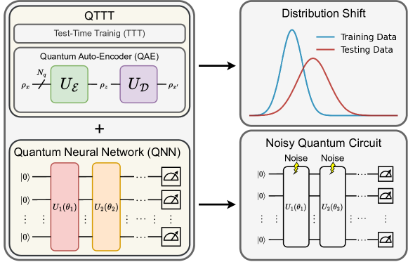
We propose test-time training with a quantum auto-encoder (QTTT) to tackle two key challenges: (1) enhancing model generalization when the distribution of training and testing data differ, and (2) enabling noise-awareness for deployment scenarios where the QML model faces noise not presenting during the training stage. QTTT deploys a Y-shaped architecture following Gandelsman et al., (2022); Sun et al., (2020). The architecture comprises a parameter-shared quantum encoder, a quantum decoder, and the main QML model for downstream tasks. During training, the multi-task objective is minimized on both the quantum auto-encoder (QAE) loss function and the classification loss function from the main QML model. At test time, the shared quantum encoder is trained on a self-supervised task by minimizing the QAE loss function for quantum state recovery. This approach leverages the idea of self-supervision to capture the underlying distribution of testing data. Moreover, our experimental results show that minimizing the self-supervised loss during testing effectively mitigates noise in quantum circuits that may not be present during training.
The QTTT framework (see Figure 1) provides a plug-and-play extension for existing QML models, addressing the challenges related to the distribution shift from training and testing data and quantum circuit error during the deployment stage. This innovative framework brings QML closer to real-world applications, accommodating deployment scenarios where quantum computers may exhibit different noise characteristics than those encountered during training.
Contributions.
We summarize our main contribution as follows:
-
•
We propose QTTT, a novel test-time training framework for QNNs, offering a plug-and-play architecture extension to address distribution shifts between training and testing data and random unitary noise during inference.
-
•
We theoretically analyze the performance guarantee of QTTT by examining the main task loss under gradient descent during test time while optimizing the shared parameters. Additionally, we present the computation overhead ratio of QTTT relative to training, which reduces when the depth of the main task model increases.
-
•
We conduct comprehensive experiments and show that (1) QTTT effectively improves the performance of QNNs on corrupted testing data and (2) QTTT robustly mitigates random unitary noises in quantum circuits.
Organizations.
We organize the paper as follows. In Section 2, we organize related works of test-time training, QNNs, and noise-aware variational quantum algorithms. We introduce the QTTT method in Section 3 and provide theoretical analysis on its performance guarantee in Section 4. In Section 5, we demonstrate the effectiveness of QTTT on addressing distribution shifts between training and testing data and mitigating quantum circuit error. Finally, we discuss the future direction and limitation of QTTT in Section 6 and conclude this paper in Section 7.
Notations.
We denote scalars and vectors in lowercase letters and matrices in uppercase letters, the -norm of vector . We use to denote the concatenation operation. The inner product of vectors and of the same dimension is denoted by .
2 Related Works
Quantum Machine Learning.
QML is often categorized into three main types (Bowles et al.,, 2024): quantum neural networks, convolutional quantum neural networks, and quantum kernel methods. QNN utilizes parameterized quantum circuits (PQCs) to encode data and evolve the quantum state, with parameter training carried out through classical optimization. Following Bowles et al., (2024), popular QNN models include the data reuploading classifier (Pérez-Salinas et al.,, 2020), dressed quantum circuits (Mari et al.,, 2020), and the quantum Boltzmann machine (Amin et al.,, 2018). On the other hand, quantum kernel methods leverage quantum computers to evaluate kernel functions, embedding classical data into quantum states to measure similarity between data points through inner products (Bowles et al.,, 2024). Following Bowles et al., (2024), popular quantum kernel methods include the IQP kernel classifier (Havlíček et al.,, 2019) and the projected quantum kernel (Huang et al.,, 2021). Finally, quantum convolutional neural networks (QCNNs) is the quantum analog of classical convolutional neural networks, incorporating inductive biases of translation invariance and locality. Examples of such models include Quantum Convolutional Neural Networks (Cong et al.,, 2019) and WeiNet (Wei et al.,, 2022).
Test-Time Training.
The idea of TTT, proposed by Sun et al., (2020), minimizes the self-supervised loss of a four-way rotation prediction task during test time to address distribution shift while preserving the model’s original performance. Later, they enhanced performance by employing a masked auto-encoder as the self-supervised task for object recognition (Gandelsman et al.,, 2022). Both Gandelsman et al., (2022); Sun et al., (2020) consider testing data arriving sequentially, framing TTT as a one-sample learning problem. Conversely, other studies have explored TTT in various applications using either the entire dataset or batches from the testing distribution (Liu et al.,, 2021; Wang et al.,, 2020). Additionally, the idea of test-time training is also employed in LLMs (Snell et al.,, 2024) and video stream (Wang et al.,, 2023).
3 Methodology
In this section, we first formulate the problem of (1) distribution shift between training and testing data and (2) quantum circuit errors during inference that are absent during training in Section 3.1. In Section 3.2, we present the architecture of QTTT and various components.
3.1 Problem Formulation
Classification Problem.
In an classification problem with class, given a feature vector of dimension and its corresponding one-hot label vector , a classifier with trainable parameters predicts the class of the input, i.e., . We use to denote the loss of the model given data pair . Given training dataset with number of data point , drawn from data distribution , the model is obtained by minimizing the empirical loss,
Distribution Shift.
Given testing data with number of data point , drawn from a different data distribution , the empirical loss is
We use QTTT to update the parameter set by performing gradient descent starting from such that .
Noisy Qunatum Cirucit.
Given testing data drawn from data distribution , we consider a noisy classifier . Then use QTTT to update the parameter set from .
3.2 QTTT Architecture
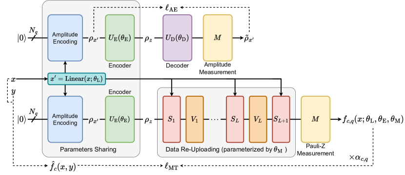
The architecture is designed to have two branches after a shared encoding block. The first branch is the decoding block, forming a quantum auto-encoder (QAE) with a shared quantum encoding block. The second branch is the main classification task block. Figure 2 shows the architecture and the calculation flow of QTTT.
Pre-Processing of Data.
To enhance the QTTT effectiveness, we first feed data into a linear layer which outputs a feature vector which will also be used many times in data re-uploading part in the classification block later, the other branch.
where , , and are the parameters in the linear layer, where means flattening the input to a row vector. Then we use amplitude encoding (Mottonen et al.,, 2004) to encode the classical data into quantum data into the quantum circuit where is the number of qubits of the quantum circuit,
where is the initial state of the muti-qubit quantum circuit.
Auto-Encoder Branch.
The encoding and decoding block are denoted as parameterized unitary operators and with trainable parameters and , respectively. The encoding block transforms the quantum state in data space to a latent variable in the latent space, and the decoding block sends the latent variable back to the data space (Romero et al.,, 2017),
The QAE loss is defined as the relative infidelity between the original data state and the recovered data state ,
Together with the linear layer in the beginning, the QAE loss is denoted as
We consider the “trash” qubits as a hyperparameter of QTTT. Specifically, we discard in the output of the quantum encoding block and use the quantum decoder to reconstruct the quantum from the “reference state”. Further discussion on the necessity of trash qubit is provided in Section 5.3.
Main Task Branch.
We select data re-uploading (Pérez-Salinas et al., (2020)) as the main task (classification) branch after the shared linear layer, amplitude encoding, and the variational encoding block. The main task block is denoted as a chain of products of parameterized unitaries,
| (3.1) |
where is the parameter vector of the main task block. We use to denote the -layer of data re-uploading layers and the -layer of the variational layer. The final state of the main task branch is denoted by ,
We measure each qubit individually and obtain the reduced density state . We introduce the relative fidelity between the single-qubit state and the single-qubit label state of class as
We use to denote the objective fidelity regarding class given data pair . The main task loss is the weighted fidelity cost function of the final quantum state as
where is the trainable class weight for qubit regarding class (Pérez-Salinas et al.,, 2020).
During the main task inference (classification), we fix the weights after training and select the class with the largest fidelity given data ,
| (3.2) |
We use parameterized unitary with three Euler angles on each qubit and follow with strong entanglement (ladder CNOT) layers for both the encoder, decoder and the main QML model. We divide the input features by three and feed them into the gates. On the other hand, QAE requires the qubit number of for amplitude encoding. Therefore, we choose the qubit number and pad feature vectors with zeros to match the qubit configurations. We run the experiment with state vector simulations. Figure 3 shows the basic blocks and Figure 4 shows the quantum circuits of the two branches shown in Figure 2.
Quantum Circuits.
Figure 3 presents the basic components of parameterized and entanglement blocks. Specifically, we present the general rotation layer and ladder entanglement layer . Each layer has parameter numbers of 3 multiples of the qubit number, and each entanglement layer has the same number of CNOT gates of the qubit number.
Figure 4 shows the overall quantum circuit implementation of QTTT. Note that each layer represents a general rotation layer followed by a ladder entanglement layer . The QAE branch and the main task branch have the same number of qubits , and is the number of trash qubits discarded after the encoder. There are additional auxiliary qubits for resetting the qubit states after the quantum encoder.
Both the QAE branch and the main task branch are quantum circuits with total qubit number . The QAE branch (top of Figure 4) consists of an encoding block and a decoding block. The first qubits encode the input data with amplitude encoding (Mottonen et al.,, 2004). The non-negative trash qubits number is a hyper-parameter smaller than . The encoder is supposed to compress the information into the first qubits and leave sparse information in the last qubits. We denote the number of layers in the encoder as .
The decoder takes both the quantum state of the first qubits out of the encoder and other qubits prepared in some reference states as input. Between the encoder and decoder blocks, the SWAP operation realizes the above process by swapping the last two registers (both with qubits). Finally, we measure the amplitude of the final quantum state out of the decoder for later calculation of the QAE loss . We denote the number of layers in the decoder as .
The main task branch (bottom of Figure 4) consists of the same encoder shared with the QAE followed by a data re-uploading block and Pauli-Z measurement at the end. We apply the Pauli-Z measurement to calculate the main task loss . The alternatively repeated and the in (3.1) is realized with the and gates, respectively. We denote the repeat number of and layers in the data re-uploading block as .
| General Rotation Layer | Ladder Entanglement Layer | |
|---|---|---|
|
{quantikz}
& \setwiretypeq\gate[5] U_3 \midstick[5,brackets=none] = \gateU_3(⋅, ⋅, ⋅)\gategroup[5,steps=1,style=dashed,rounded corners, fill=gray_block, inner xsep=2pt,background,label style=label position=below,anchor=north,yshift=-0.2cm] \setwiretypeq \gateU_3(⋅, ⋅, ⋅) \setwiretypeq \gateU_3(⋅, ⋅, ⋅) ⋮\setwiretypen ⋮ ⋮ \setwiretypeq \gateU_3(⋅, ⋅, ⋅) |
{quantikz}
& \setwiretypeq\gate[5] E \midstick[5,brackets=none] = \ctrl1\gategroup[5, steps=4,style=dashed,rounded corners, fill=gray_block, inner xsep=2pt,background,label style=label position=below,anchor=north,yshift=-0.2cm] \ghostU_3 … \targ \setwiretypeq \targ \ctrl1 … \ghostU_3 \setwiretypeq \targ … \ghostU_3 ⋮\setwiretypen ⋮ ⋮ … \ghostU_3 \setwiretypeq \ghostU_3 … \ctrl-4 |
|
{quantikz}\lstick
&\qwbundleN_q-N_t \gate[wires=2, style=fill=blue_ampEncoding,label style=black]Amplitude Encoding \gate[wires=2, style=fill=orange_v]U_3&E\gategroup[2,steps=3,style=dashed,rounded corners, fill=green_encoder, inner xsep=2pt,background,label style=label position=above,anchor=north,yshift=+0.4cm]Encoder \gate[wires=2, style=fill=orange_v]U_3&E … \gate[wires=2, style=fill=orange_v]U_3&E\gategroup[2,steps=3,style=dashed,rounded corners, fill=blue!20, inner xsep=2pt,background,label style=label position=above,anchor=north,yshift=+0.4cm]Decoder \gate[wires=2, style=fill=orange_v]U_3&E … \meter\gategroup[2,steps=1,style=dashed,rounded corners, fill=yellow_measure, inner xsep=2pt,background,label style=label position=above,anchor=north,yshift=+0.4cm] \lstick \qwbundleN_t … \swap1 … \meter \lstick \qwbundleN_t \targX \meter |
|
{quantikz}\lstick
&\qwbundleN_q-N_t \gate[wires=2, style=fill=blue_ampEncoding,label style=black]Amplitude Encoding \gate[wires=2, style=fill=orange_v]U_3&E\gategroup[2,steps=3,style=dashed,rounded corners, fill=green_encoder, inner xsep=2pt,background,label style=label position=above,anchor=north,yshift=+0.4cm]Encoder \gate[wires=2, style=fill=orange_v]U_3&E … \gate[wires=2, style=fill=pink_dru]U_3\gategroup[2,steps=5,style=dashed,rounded corners, fill=gray_block, inner xsep=2pt,background,label style=label position=above,anchor=north,yshift=+0.4cm]Data Re-uploading \gate[wires=2, style=fill=orange_v]U_3&E \gate[wires=2, style=fill=pink_dru]U_3 \gate[wires=2, style=fill=orange_v]U_3&E … \meter\gategroup[2,steps=1,style=dashed,rounded corners, fill=yellow_measure, inner xsep=2pt,background,label style=label position=above,anchor=north,yshift=+0.4cm] \lstick \qwbundleN_t … \swap1 … \meter \lstick \qwbundleN_t \targX \meter |
Multi-Task Loss.
The total loss function is defined as the weighted sum of the main task loss and the QAE loss :
where , and are trainable log-variance parameters for multi-task learning (Kendall et al.,, 2018). The purpose of and is weighting to balance between multi-task loss according to the noise level. Following Kendall et al., (2018), by maximizing the Gaussian likelihood, the model learns to scale the losses for each output. A larger represents a larger variance, thereby reducing the contribution of this task during optimization and vice versa.
Multi-Tasks Training.
We minimize the following total loss on training dataset with number of data point while training:
| (3.3) |
Test-Time Training.
After the regular training is completed, we fix the trained parameters and in the main task branch. On the other hand, we initialize the encoder and decoder parameters with and update them using gradient descent to to minimize the following QAE self-supervised loss:
| (3.4) |
By Theorem 4.1, a one-step gradient descent on the QAE loss lowers the main task loss, we can deduce that minimizing the QAE loss (3.4) during test-time training improves the performance of the model on the main task.
4 Theoretical Analysis
In this section, we provide the theoretical analysis of our proposed methodology in Section 3. Specifically, in Theorem 4.1 we prove that under convex, smooth, and bounded loss functions, a one-step gradient during test time further lowers the main task loss. In Table 1, we analyze the computational complexity of QTTT to quantify the computation overhead ratio between QTTT test-time training and standard training.
For clarity and fluency, we state some notations before stating the theorem. Because parameters and are parts of the encoding block the two branches share, we combine them and let . Because in the following derivation, we focus on and the gradient of the loss functions with respect to it, we neglect other irrelevant parameters without causing ambiguity.
Theorem 4.1.
Let denote the main task loss on a test data point , and the self-supervised auto-encoder task loss, which depends only on . Here, represents the shared parameters. Assume that for all , main task loss is differentiable, convex, and -smooth with respect to , and that both gradients are bounded.
| (4.1) |
With a fixed learning rate , for every there exist such that
| (4.2) |
Therefore, we have
| (4.3) |
where , i.e., Test-Time Training with one step of gradient descent.
Remark 4.1 (Test-Time Training).
With a convex, smooth, and bounded loss function, we show that the main task loss on the testing dataset is further lowered when we first optimize all the parameters on the training data and then “fine-tune” the self-supervised QAE parameters on the testing data, that is
Proof of Theorem 4.1.
Our proof is based on Sun et al., (2020). Given data point pair , we expand the main task loss at to the second order,
| (4.4) |
Taking the step vector and the step size :
| (4.5) | ||||
| (4.6) |
We write (4.4) as
| (4.7) |
where the last inequality (4.7) is from (4.1) and (4.2). Rearranging (4.7), we have
| (4.8) |
Let . By convexity of we have
Combining with (4.8), we have
Since , we have
| (4.9) |
This completes the proof. ∎
Computational Complexity.
We summarize the computational complexity for each component of QTTT in Table 1. We calculate the gradient of the PQC with the parameter-shift rule. We treat the number of gate operations as the basic unit, assuming all gates operate individually and separately, and neglect the classical computation before and after the quantum circuits. Here, we use the same notation as introduced in the main paper: represent the number of training data, the number of testing data, the number of qubits, the number of layers of the encoder, the number of layers of the decoder, the number of layers of the data re-uploading block in the main task branch, and is the total number of measurement shots. From Table 1, the proportion of training gate complexity (time complexity) for computing gradient with TTT is . For example, assuming the overhead for QTTT is of the ratio , with the testing data generally being a small portion compared to the training data. Notably, the overhead ratio of TTT scales is inversely proportional to the main task model depth , meaning that the deeper the models, the smaller the overhead ratio, making QTTT an ideal plug-and-play framework for other QML models.
| Aspect | Gate Complexity |
|---|---|
| Gradient Calculation (Training) | |
| Gradient Calculation (QTTT) |
5 Experiments
In this section, we demonstrate QTTT’s ability to (1) tackle distribution shifts in the testing data and (2) mitigate random unitary noise in quantum circuits during inference. We select four QML models as the baseline from the top performance models reported by the benchmark paper (Bowles et al.,, 2024). It consists of two variational QML models: data reuploading classifier (Pérez-Salinas et al.,, 2020) and dressed quantum circuit (Mari et al.,, 2020); two kernel-based QML models: IQP kernel classifier (Havlíček et al.,, 2019) and projected quantum kernel (Huang et al.,, 2021). In our experimental setup, we set the quantum circuit layers (see Figure 4).
Our experiments are organized into the following three parts, respectively showing:
-
•
QTTT demonstrates robustness against data corruption, including Gaussian noise, brightness variations, fog, and snow effects, outperforming the state-of-the-art QML model (see Section 5.1).
-
•
QTTT mitigates simple random unitary noise in quantum circuits at test time, paving the way for a new noise-aware architecture design in QML models as well as a plug-and-play extension for existing QML models (see Section 5.2).
-
•
We conduct ablation studies to verify the effectiveness of QTTT architectural design (see Section 5.3).
5.1 Distribution Shift
We follow the data corruption settings from Gandelsman et al., (2022); Sun et al., (2020) and implement the baseline models and datasets from the benchmark paper (Bowles et al.,, 2024). For details on the dataset generation process, see Bowles et al., (2024); the datasets consist of samples with a training/testing split of .
Setup.
We select top-performance QML models based on the benchmark results in Bowles et al., (2024). We follow the model training settings for QTTT and the baseline QML models. These five synthetic datasets include linear separable, hidden manifold, two curves, hyperplanes, bar & stripes (Bowles et al.,, 2024). We exclude the MNIST data since it either needs to drastically downsize the image or perform PCA to reduce feature dimensions. We average the results over the five kinds of datasets with three random seeds for each, hence 15 experiments for each. We select the datasets with feature dimensions and , and the corresponding qubits number is and , respectively. For both experiments, we choose . Here, we summarize the four corruptions we employ in this section.
-
(C1)
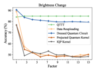
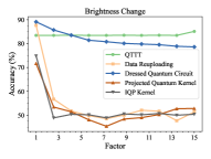
Brightness Change. We change the brightness of the data by perturbing the testing data by a factor, i.e., .
-
(C2)
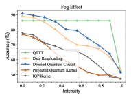
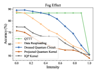
Fog Effect. We apply the fog effect on data by perturbed testing data, .
-
(C3)
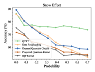
Snow Effect. We apply the snow effect on data by adding random noise (uniform distribution) to each feature with probability .
-
(C4)
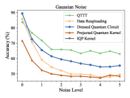
Gaussian Noise. We add Gaussian noise to the testing sets by perturbing the testing data with noise sampled from the normal distribution. Specifically, the noise added to each element of , the final pertubed data is computed as .
Results.
In Figure 5, we demonstrate the model accuracy on the testing datasets under different data corruptions. For Figure 5a to Figure 5d we use the dataset with feature dimension . For Figure 5e to Figure 5h we use . For Figure 5d, the accuracy consistently outperforms all baseline QML methods when adding Gaussian noise. For Figures 5a, 5b and 5c, QTTT exhibits more robustness against increasing corruption levels. Remarkably, with increasingly corrupted data, QTTT still maintains its performance while others drop off rapidly. However, the QTTT performance on original uncorrupted data is slightly lower than that of the data reuploading classifier and dressed quantum circuit. The slight performance drop is due to the multi-task learning from two objectives: minimizing the self-supervised loss and minimizing the main classification task loss.
 (a) Brightness Change.
 (b) Fog Effect.
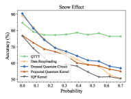 (c) Snow Effect.
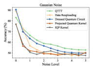 (d) Gaussian Noise.
 (e) Brightness Change.
 (f) Fog Effect.
 (g) Snow Effect.
 (h) Gaussian Noise.
5.2 Noisy Quantum Circuit
In a real-world application scenario, the QML model is trained on a noise-free quantum computer, while the inference can be performed on a noisy quantum computer. The QML model needs to be robust against quantum circuit errors. In this section, we demonstrate QTTT’s ability to mitigate a simple noise model, specifically random unitary noise.
Setup.
After each layer, we apply a rotation gate randomly sampled from with equal probability on each qubit, with each rotation angle sampled from . We use data re-uploading as the baseline for this experiment and follow the same experimental setup and training setting as described in Section 5.1. We choose for the experiment. We still average the results over the five kinds of datasets ten random seeds, hence 50 experiments for each noise level. Note that all models are trained in a noise-free setting. However, the random unitary noise described above is applied during inference. We examine both batch and online versions of QTTT, where data is provided either in batches or sequentially.
Results.
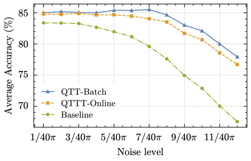
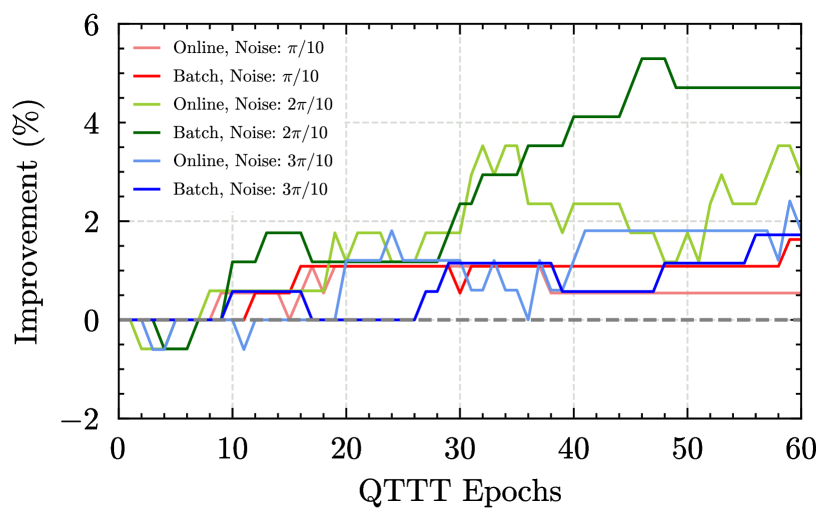
In Table 2, we summarize the performance of QTTT and the baseline models in noisy quantum circuits under increasing circuit noise levels. QTTT with batch optimization during test time achieves a improvement on average in noisy circuit settings. Meanwhile, the online version of QTTT still achieves an improvement of , despite only “overfitting” on a single test sample. QTTT offers a plug-and-play extension for existing QML models when inference on a noisy quantum circuit. We demonstrate that QTTT mitigates the simple random unitary noise and improves the performance by up to . In Figure 6, we visualize the average accuracy of increasing noise levels and the improvement of the model accuracy with three noise levels over test-time training epochs.
| Mean | |||||||||||||
|---|---|---|---|---|---|---|---|---|---|---|---|---|---|
| Data Re-uploading | 83.374 | 83.351 | 83.281 | 82.665 | 81.967 | 81.167 | 79.604 | 77.606 | 74.927 | 72.879 | 70.036 | 67.534 | 78.199 |
| QTTT-Online | 84.802 | 84.756 | 84.893 | 84.653 | 84.678 | 84.463 | 84.052 | 83.525 | 81.702 | 80.675 | 78.579 | 76.698 | 82.790 |
| QTTT-Batch (Default) | 85.007 | 85.178 | 85.053 | 85.001 | 85.404 | 85.378 | 85.511 | 84.656 | 83.016 | 82.095 | 79.996 | 77.93 | 83.685 |
5.3 Ablation Studies
We compare the model accuracy for batch and online learning and the trash qubit number of the QAE (see details in Section 3). We also conduct comprehensive ablation studies on QTTT and validate the QTTT configuration setups. We follow the same experimental setup and training setting described in Section 5.1 and choose . The results are summarized in Table 3, where the top half compares various QTTT configurations such as batch learning, online learning, trash qubit number and , and for the bottom half we remove various components of QTTT as ablation study, including removing test-time training, the linear layer, data reuploading in the main task branch, and the multi-task loss (see Section 3). We average the model accuracy over the experiments.
The results in Table 3 indicate that either the default or a moderate number of trash qubits yields better model performance across various corruptions and quantum circuit errors. Additionally, we verified the effectiveness of our architectural design by examining various components of QTTT, including test-time training, the linear layer, data reuploading in the main task branch, and multi-task objective training.
| Brightness | Fog | Snow | Gaussian | Mean | ||||
|---|---|---|---|---|---|---|---|---|
| QTTT-Batch (Default) | 86.88 | 86.94 | 73.23 | 52.59 | 85.00 | 84.66 | 77.93 | 78.18 |
| QTTT w/ | 87.40 | 87.40 | 72.72 | 54.40 | 83.80 | 73.42 | 65.88 | 75.00 |
| QTTT w/ | 87.83 | 81.67 | 71.64 | 53.39 | 86.73 | 76.96 | 67.43 | 75.09 |
| QTTT-Online | 47.45 | 47.47 | 43.44 | 30.52 | 86.72 | 72.17 | 66.70 | 56.35 |
| w/o TTT | 85.73 | 75.83 | 58.31 | 50.40 | 83.38 | 62.93 | 56.69 | 67.61 |
| w/o Linear Layer | 84.20 | 84.20 | 71.26 | 49.93 | 74.58 | 59.59 | 52.90 | 68.09 |
| w/o Data Reuploading | 63.63 | 63.63 | 62.33 | 49.07 | 66.58 | 59.24 | 56.02 | 60.07 |
| w/o Multi-Task Loss | 86.70 | 86.73 | 72.82 | 52.40 | 87.81 | 73.21 | 62.93 | 74.66 |
6 Limitations and Future Works.
To facilitate the real-world application of QML models, future studies can explore more sophisticated QTTT architectures and other self-supervised tasks beyond quantum auto-encoders by quantum state recovery. Moreover, the current test-time training optimization relies on first-order gradient descent. Employing higher-order or quantum-aware optimizers (Huang and Goan,, 2024; Stokes et al.,, 2020; Gacon et al.,, 2021) could enhance its performance. While we experiment with QTTT under various data corruptions and quantum circuit noise levels, benchmarking with more advanced noise models will further support the real-world deployment of QTTT on actual quantum hardware. Additionally, a theoretical understanding of the trainability of QTTT and its limitations in a noisy setting would be valuable.
7 Conclusion
In this paper, we introduce QTTT, a novel QML framework designed for future real-world applications. QTTT serves as a plug-and-play extension for existing QML models. QTTT demonstrates robustness to distribution shifts between training and testing data, as well as mitigating simple quantum circuit noise during inference. This is achieved by minimizing the self-supervised loss of a quantum auto-encoder. Empirically, we show that QTTT outperforms existing QML models on corrupted data and random unitary noise introduced at test time. Theoretically, we provide performance guarantees for QTTT and analyze its computational complexity, showing its minor overhead with increased quantum model depth.
However, scaling up QML in the NISQ era poses challenges in demonstrating whether it offers advantages over classical counterparts. These challenges include the expressiveness and trainability of QML models, as well as error mitigation on real quantum hardware. Our work takes a small step toward unlocking real-world applications of QML in the NISQ era, providing a novel noise-aware framework for existing QML models.
Acknowledgements
H.-S.G. acknowledges support from the National Science and Technology Council, Taiwan under Grants No. NSTC 113-2112-M-002-022-MY3, No. NSTC 113-2119-M-002 -021, No. NSTC112-2119-M-002-014, No. NSTC 111-2119-M-002-007, and No. NSTC 111-2627-M-002-001, from the US Air Force Office of Scientific Research under Award Number FA2386-23-1-4052 and from the National Taiwan University under Grants No. NTU-CC-112L893404 and No. NTU-CC-113L891604. H.-S.G. is also grateful for the support from the “Center for Advanced Computing and Imaging in Biomedicine (NTU-113L900702)” through The Featured Areas Research Center Program within the framework of the Higher Education Sprout Project by the Ministry of Education (MOE), Taiwan, and the support from the Physics Division, National Center for Theoretical Sciences, Taiwan.
References
- Abbas et al., (2021) Abbas, A., Sutter, D., Zoufal, C., Lucchi, A., Figalli, A., and Woerner, S. (2021). The power of quantum neural networks. Nature Computational Science, 1(6):403–409.
- Amin et al., (2018) Amin, M. H., Andriyash, E., Rolfe, J., Kulchytskyy, B., and Melko, R. (2018). Quantum boltzmann machine. Physical Review X, 8(2):021050.
- Bowles et al., (2024) Bowles, J., Ahmed, S., and Schuld, M. (2024). Better than classical? the subtle art of benchmarking quantum machine learning models. arXiv preprint arXiv:2403.07059.
- Cong et al., (2019) Cong, I., Choi, S., and Lukin, M. D. (2019). Quantum convolutional neural networks. Nature Physics, 15(12):1273–1278.
- Gacon et al., (2021) Gacon, J., Zoufal, C., Carleo, G., and Woerner, S. (2021). Simultaneous perturbation stochastic approximation of the quantum fisher information. Quantum, 5:567.
- Gandelsman et al., (2022) Gandelsman, Y., Sun, Y., Chen, X., and Efros, A. (2022). Test-time training with masked autoencoders. Advances in Neural Information Processing Systems, 35:29374–29385.
- Havlíček et al., (2019) Havlíček, V., Córcoles, A. D., Temme, K., Harrow, A. W., Kandala, A., Chow, J. M., and Gambetta, J. M. (2019). Supervised learning with quantum-enhanced feature spaces. Nature, 567(7747):209–212.
- Herrmann et al., (2022) Herrmann, J., Llima, S. M., Remm, A., Zapletal, P., McMahon, N. A., Scarato, C., Swiadek, F., Andersen, C. K., Hellings, C., Krinner, S., et al. (2022). Realizing quantum convolutional neural networks on a superconducting quantum processor to recognize quantum phases. Nature communications, 13(1):4144.
- Huang et al., (2021) Huang, H.-Y., Broughton, M., Mohseni, M., Babbush, R., Boixo, S., Neven, H., and McClean, J. R. (2021). Power of data in quantum machine learning. Nature communications, 12(1):2631.
- Huang and Goan, (2024) Huang, Y.-C. and Goan, H.-S. (2024). L2O-g†: Learning to Optimize Parameterized Quantum Circuits with Fubini-Study Metric Tensor. arXiv preprint arXiv:2407.14761.
- Kendall et al., (2018) Kendall, A., Gal, Y., and Cipolla, R. (2018). Multi-task learning using uncertainty to weigh losses for scene geometry and semantics. In Proceedings of the IEEE conference on computer vision and pattern recognition, pages 7482–7491.
- Larocca et al., (2023) Larocca, M., Ju, N., García-Martín, D., Coles, P. J., and Cerezo, M. (2023). Theory of overparametrization in quantum neural networks. Nature Computational Science, 3(6):542–551.
- Liu et al., (2021) Liu, Y., Kothari, P., Van Delft, B., Bellot-Gurlet, B., Mordan, T., and Alahi, A. (2021). Ttt++: When does self-supervised test-time training fail or thrive? Advances in Neural Information Processing Systems, 34:21808–21820.
- Mari et al., (2020) Mari, A., Bromley, T. R., Izaac, J., Schuld, M., and Killoran, N. (2020). Transfer learning in hybrid classical-quantum neural networks. Quantum, 4:340.
- Mottonen et al., (2004) Mottonen, M., Vartiainen, J. J., Bergholm, V., and Salomaa, M. M. (2004). Transformation of quantum states using uniformly controlled rotations. arXiv preprint quant-ph/0407010.
- Pérez-Salinas et al., (2020) Pérez-Salinas, A., Cervera-Lierta, A., Gil-Fuster, E., and Latorre, J. I. (2020). Data re-uploading for a universal quantum classifier. Quantum, 4:226.
- Romero et al., (2017) Romero, J., Olson, J. P., and Aspuru-Guzik, A. (2017). Quantum autoencoders for efficient compression of quantum data. Quantum Science and Technology, 2(4):045001.
- Shor, (1997) Shor, P. W. (1997). Polynomial-time algorithms for prime factorization and discrete logarithms on a quantum computer. SIAM Journal on Computing, 26(5):1484–1509.
- Snell et al., (2024) Snell, C., Lee, J., Xu, K., and Kumar, A. (2024). Scaling llm test-time compute optimally can be more effective than scaling model parameters. arXiv preprint arXiv:2408.03314.
- Stokes et al., (2020) Stokes, J., Izaac, J., Killoran, N., and Carleo, G. (2020). Quantum natural gradient. Quantum, 4:269.
- Sun et al., (2024) Sun, Y., Li, X., Dalal, K., Xu, J., Vikram, A., Zhang, G., Dubois, Y., Chen, X., Wang, X., Koyejo, S., et al. (2024). Learning to (learn at test time): Rnns with expressive hidden states. arXiv preprint arXiv:2407.04620.
- Sun et al., (2020) Sun, Y., Wang, X., Liu, Z., Miller, J., Efros, A., and Hardt, M. (2020). Test-time training with self-supervision for generalization under distribution shifts. In International conference on machine learning, pages 9229–9248. PMLR.
- Wang et al., (2020) Wang, D., Shelhamer, E., Liu, S., Olshausen, B., and Darrell, T. (2020). Tent: Fully test-time adaptation by entropy minimization. arXiv preprint arXiv:2006.10726.
- Wang et al., (2023) Wang, R., Sun, Y., Gandelsman, Y., Chen, X., Efros, A. A., and Wang, X. (2023). Test-time training on video streams. arXiv preprint arXiv:2307.05014.
- Wei et al., (2022) Wei, S., Chen, Y., Zhou, Z., and Long, G. (2022). A quantum convolutional neural network on nisq devices. AAPPS Bulletin, 32:1–11.
- Wen et al., (2024) Wen, J., Huang, Z., Cai, D., and Qian, L. (2024). Enhancing the expressivity of quantum neural networks with residual connections. Communications Physics, 7(1):220.