Re-entrant topological order in strongly correlated nanowire due to Rashba spin-orbit coupling

Abstract

The effect of the Rashba spin orbit coupling (RSOC) on the topological properties of the one-dimensional (1D) extended s-wave superconducting Hamiltonian, in the presence of strong electron-electron correlation, is investigated. It is found that a non-zero RSOC increases the periodicity of the effective Hamiltonian, which results in the folding of the Brillouin zone (BZ), and consequently in the emergence of an energy gap at the boundary of the BZ. If the chemical potential is inside the energy gap and it does not perceive the two-band structure of the resulting energy spectrum the topological phase is removed from the phase diagram.In contrast, if we move the chemical potential upwards towards the highest occupied band the opposite happens and the non-trivial topology is restored. This is the origin of re-entrant nature of the existent topological properties. This property of the system allows us to drive the system in and out of the topological phase only by the proper tuning of the chemical potential. A heterostructure involving van der Waals materials and a 1D Moire pattern for an investigation of the predicted effect has also been proposed and discussed in our work.

I Introduction

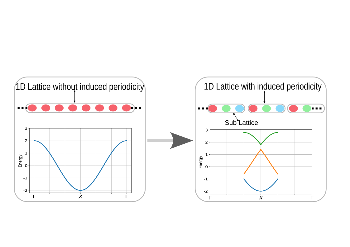
(a)

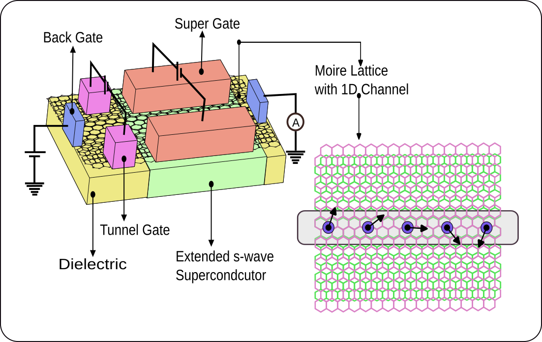
(b)

Figure 1: (a) The schematics of the energy dispersion of the non-interacting electrons in a 1D chain with (right) and without (left) a three fold periodicity of the lattice. The three fold periodicity results in the folding of the energy dispersion three times and, consequently, in the emergence of the energy gap at the BZ boundaries. If the chemical potential lies within this gap and no other band is involved no topological phase is present. On the right hand side diagram, the tuning of the chemical potential from the lower to the higher band will result in the re-entrant topological order. However, this is absent on the left hand side diagram, as there is no energy gap. (b) Schematics of the proposed heterostructure involving (quasi-)1D Moire lattice for detection of the re-entrant topological phase in strongly correlated system (discussed in Sec. VII).

The prediction of spatially separated Majorana fermions (MF) in a 1D topological superconductor (TSC) [1] has marked the paradigm shift in the research for the realization of quantum computers [2]. Several experimental platforms have been proposed to realize MF [3, 4]; among them heterostructures of a semiconducting nanowire (NW) on top of a $s$-wave SC have got a special attention, mainly due to the ease of synthesis and widespread availability of the constituent materials [5]. Three ingredients are necessary for such NW/SC heterostructures: (i) the RSOC ($\alpha$), (ii) an external magnetic field ($B_{z}$), (iii) the proximity induced s-wave superconducting (SC) order parameter ($\Delta$). The RSOC shifts the momentum parabola sideways locking the electron spin with momentum ($k$), $B_{z}$ opens a gap at $k=0$, and $\Delta$ opens a gap at opposite Fermi points.

Experimental efforts involving NW/SC have been partially fruitful and are still ongoing [6, 4, 7]. Some of the major concerns regarding NW/SC heterostructures are as follows. The critical field ($H_{c2}$) and the critical temperature ($T_{c}$) of the usual $s$-wave SC are small. Low $H_{c2}$ requires a large Lande $g$ factor in a nanowire so that a large enough gap can be opened at $k=0$ under such lower magnetic field $B_{z}<H_{c2}$. A large $\alpha$ in NW is desirable as it allows for stronger spin and momentum locking. From the design point of view, the presence of a magnetic field in electronic circuits is far from ideal, as stray fields hamper the miniaturization of the circuit. The interface between the NW and the SC should be both of high quality (allowing for a higher proximity induced SC gap) and smooth (to suppress disorder induced scattering which is detrimental for $p$-wave SC). Although, the latter concerns are of a more applied nature, however, the former (i.e., the large $\alpha$, $g$) is more of fundamental. Hence, the question arises, whether the requirements for having both RSOC and magnetic field can be completely avoided?

A number of alternative platforms have been proposed which don’t require neither RSOC nor magnetic field. Some of them are associated with atop of a magnetic atomic chain on a SC [8], topological insulator/magnetic insulator/SC heterostructure [9], monolayers of WTe₂ [10], van der Waals (vdW) materials [11, 12, 13]. Another interesting proposal is to use strong electron-electron (e-e) correlation, in place of a magnetic field, to access the topological SC phase [14, 15, 16, 17, 18]. Using DMRG it was found that strong e-e correlation favors the formation of the MF even without magnetic field [14, 15]. This favorable scenario can be easily understood in the context of a 1D chain with a single valence electron at every atomic site. Under a magnetic field the spin of every electron is frozen along the direction of the applied field. This results in every atomic site containing at most a single electron, the so called "no double occupancy" (NDO) condition. The NDO scenario can also appear due to strong e-e correlation, as the energy penalty for placing one more electron at an already occupied atomic site will be too high for that to take place; of course there is a caveat: the spin is not automatically frozen along a single direction in this case. One way to solve this problem is to invoke the so-so called "spin-charge separation" method [19]. Due to the strong e-e interaction the electron-hole excitations delocalize the electron until it becomes totally incoherent. As a result, at low energy, for this strong coupling regime, only separate non interacting collective spin (spinon) and charge (holon) excitations remains.

Although e-e correlation is an intrinsic property of the material, but several recent proposals have been put forward to control it extrinsically [20, 21, 22]. With these considerations, in this article we investigate the Hamiltonian of a (quasi-)1D topological SC system in the presence of strong e-e correlation. The SC order parameter is of extended s-wave; proximity induced due to iron based SC. The reason for choosing iron-based SC is because they have higher $T_{c}$, $H_{c2}$ and superconducting gap [23]. In the Hamiltonian we also included RSOC and magnetic field to understand their affect on the topological properties; although, the overall goal is to get rid of them. To solve the Hamiltonian we use spin-charge separation and $su(2|1)$ path integral method [[][;seeforreviewofthemehod], 24]. This method has been applied to several other systems [25, 26, 27, 28, 18, 29].

The main results of this work is as follows. (i) For non-zero RSOC the system can enter into the topological phase multiple times when the parameters are appropriately tuned (see Fig. 2). This happens due to the folding of the Brillouin zone (BZ), which takes place because of the quasi-periodicity induced by the non-zero RSOC as shown schematically in Fig. 1a. The same property was also observed in Ref. [13] due to Moire potential. (ii) The effective Hamiltonian, Eq. (11), contains the dynamical parameter $\theta$, which is a function of spinon degree of freedom — they are related through Eq. (9) and Eq. (6). For system to be in topological phase the two conditions should be satisfied, firstly the value of $\theta$ should be $0<\theta<\pi$, secondly the $\mathbb{Z}_{2}$ invariant should be $Q=-1$. From free energy calculation (Fig. 6) we find that both these conditions can be satisfied in some defined range of chemical potential. Therefore only the chemical potential can be used as the tuning parameter to drive the system into and out of the topological phase. It is useful for the design of the devices where chemical potential can be controlled efficiently through gate voltage. (iii) We propose heterostructure involving vdW materials for experimental realization of the effect; a schematic diagram of the same is shown in Fig. 1b. We discuss about this heterostructure thoroughly in Sec. VII.

II Model

We consider an effective Hamiltonian of a 1D strongly correlated SC nanowire under an externally applied magnetic field with Rashba spin-orbit coupling (RSOC):

$$H= \left[X_{i}^{0\sigma}\right]^{\dagger}\left(-t\tau_{0}-\alpha\tau_{y}\right)\left[X_{i+1}^{0\sigma}\right]-\imath\left[X_{i}^{0\sigma}\right]^{\dagger}\Delta\tau_{y}\left[X_{i+1}^{\sigma 0}\right]$$ (1)

$$\quad+\text{H.c.}+\left[X_{i}^{0\sigma}\right]^{\dagger}\left(\mu\tau_{0}+B_{z}\tau_{z}\right)\left[X_{i}^{0\sigma}\right].$$

Here, $\sigma=\ket{\uparrow},\ket{\downarrow}$ is the spin projection; $\tau_{i=0,x,y,z}$ are the Pauli matrices; $t$ is the electron hopping energy, $\alpha$ is the RSOC strength; $\mu$ is the chemical potential; $B_{z}$ is the externally applied magnetic field along $z$-axis; $\Delta$ is the extended $s$-wave SC order parameter. $\left[X_{i}^{0\sigma}\right]^{\dagger}$ are the row matrices $\left(X_{i}^{\uparrow 0},X_{i}^{\downarrow 0}\right)$. $X_{i}^{pq}$ is the Hubbard operator representing transition from $\ket{q}$ to $\ket{p}$ state at $i$-th site. In terms of usual fermion creation $\left(c_{i\sigma}^{\dagger}\right)$, annihilation $\left(c_{i\sigma}\right)$ and number operators $\left(n_{i\sigma}=c_{i\sigma}^{\dagger}c_{i\sigma}\right)$ it reads:

$$X_{i}^{0\sigma}=(1-n_{i\sigma^{\prime}})c_{i\sigma},\quad X_{i}^{\sigma 0}=c_{i\sigma}^{\dagger}(1-n_{i\sigma^{\prime}}).$$ (2)

These definitions allow us to project out the doubly occupied states.

Using coherent-state symbols of $X_{i}^{\sigma\sigma^{\prime}}$ operators and after successive transformations Eq. (1) reads (see Ref. [18, 29] for more elaborate mathematical treatment):

$$H_{\text{eff}}(z,\xi)= -\sum\limits_{i}\xi_{i+1}\bar{\xi}_{i}\left(t\>a_{i}+\imath\alpha\>\alpha_{i}\right)-\Delta\sum\limits_{i}\bar{\xi}_{i+1}\bar{\xi}_{i}\>\Delta_{i}$$ (3)

$$\quad+\text{H.c.}+\sum\limits_{i}\xi_{i}\bar{\xi}_{i}\left(\mu+B_{z}\beta_{i}\right),$$

where,

$$a_{i}\equiv\frac{1+\bar{z}_{i+1}z_{i}}{\sqrt{\left(1+\left|z_{i+1}\right|^{2}\right)\left(1+\left|z_{i}\right|^{2}\right)}},\alpha_{i}\equiv\frac{\bar{z}_{i+1}-z_{i}}{\sqrt{\left(1+\left|z_{i+1}\right|^{2}\right)\left(1+\left|z_{i}\right|^{2}\right)}},$$ (4)

$$\Delta_{i}\equiv\frac{z_{i}-z_{i+1}}{\sqrt{\left(1+\left|z_{i}\right|^{2}\right)\left(1+\left|z_{i+1}\right|^{2}\right)}},\beta_{i}\equiv\frac{1-\left|z_{i}^{2}\right|}{1+\left|z_{i}^{2}\right|}.$$

The fractionalization of the spin (spinon, $z_{i}$) and charge (holon, $\xi_{i}$) degrees of freedom in Eq. (3) allows them to be treated on the same footing. $a_{i}$, $\alpha_{i}$, $\Delta_{i}$ and $\beta_{i}$ are functions of $z_{i}$, which renders these coefficients spatially dependent.

The coherent state $su(2)$ generators of the three spin components in terms of $z_{i}$ are [25, 24]:

$$S_{i}^{+}=\frac{z_{i}}{1+\left|z_{i}\right|^{2}},\quad S_{i}^{-}=\frac{\bar{z}_{i}}{1+\left|z_{i}\right|^{2}},\quad S_{i}^{z}=\frac{1}{2}\left(\frac{1-\left|z_{i}\right|^{2}}{1+\left|z_{i}\right|^{2}}\right).$$ (5)

Here, $S_{i}^{x}=S_{i}^{+}+S_{i}^{-}$ and $S_{i}^{y}=-\imath\left(S_{i}^{+}-S_{i}^{i}\right)$. As $z_{i}$ is a $c$-number, in Cartesian form its real and imaginary parts are:

$$\real z_{i}=S_{i}^{x}\left(1+\frac{1-2S_{i}^{z}}{1+2S_{i}^{z}}\right),\quad\imaginary z_{i}=S_{i}^{y}\left(1+\frac{1-2S_{i}^{z}}{1+2S_{i}^{z}}\right).$$ (6)

In polar form

$$z_{i}=\left(1+\frac{1-2S_{i}^{z}}{1+2S_{i}^{z}}\right)\sqrt{\left(S_{i}^{x}\right)^{2}+\left(S_{i}^{y}\right)^{2}}\exp\left[\imath\arctan\left(S_{i}^{y}/S_{i}^{x}\right)\right]$$ (7)

Given a $c$-number $z_{i}$, using Eq. (5) the su(2) spin components $S_{i}^{x}$, $S_{i}^{y}$, and $S_{i}^{z}$ can be found immediately. Similarly, given three su(2) spin components the corresponding $c$-number $z_{i}$ can be found either using Eq. (6) or Eq. (7).

For a ferromagnetic (FM) spinon configuration all the spins are aligned along the $z$-axis:

$$\vec{S}_{i}=\left(S_{i}^{x},S_{i}^{y},S_{i}^{z}\right)=\frac{1}{2}\left(0,0,1\right).$$ (8)

Substituting Eq. (8), first in Eq. (6), and then the result of that in Eq. (4), we find that only $a_{i}$ and $\beta_{i}$ are non-zero . The effective Hamiltonian, Eq. (3), reduces to usual 1D NW without SC order. Hence, FM configuration is not of our interest. The antiferromagnetic spinon configuration will also give the same result . However, spiral spinon field is different. The spatially dependent spinon configuration having only x-y plane projection reads

$$\vec{S}_{i}=\left(S_{i}^{x},S_{i}^{y},S_{i}^{z}\right)=\frac{1}{2}\left(\cos\theta_{i},\sin\theta_{i},0\right).$$ (9)

Here the $S_{i}^{z}$ component of the spinon is zero and $\theta_{i}$ is spatially dependent. The corresponding $c$-number obtained from Eq. (7) is $z_{i}=\mathrm{e}^{\imath\theta_{i}}$. Substituting this $z_{i}$ in Eq. (4) we find:

$$a_{i}=\mathrm{e}^{-\imath\left(\theta_{i+1}-\theta_{i}\right)/2}\cos\frac{\left(\theta_{i+1}-\theta_{i}\right)}{2},\quad\beta_{i}=0,$$ (10)

$$\alpha_{i}=-\imath\mathrm{e}^{-\imath\left(\theta_{i+1}-\theta_{i}\right)/2}\sin\frac{\left(\theta_{i+1}+\theta_{i}\right)}{2},$$

$$\Delta_{i}=-\imath\mathrm{e}^{\imath\left(\theta_{i+1}-\theta_{i}\right)/2}\sin\frac{\left(\theta_{i+1}-\theta_{i}\right)}{2}\mathrm{e}^{\imath\theta_{i}}.$$

For a spiral spinon field the change in the $\theta_{i}$ from neighboring sites is, i.e. $\theta_{i+1}-\theta_{i}=\theta$. Using this fact in Eq. (10), substituting the resulting expressions in Eq. (3), and making the gauge transformation $\xi_{i}\to\xi_{i}\mathrm{e}^{\imath(\theta_{i}/2-\pi/4)}$, we get the Hamiltonian with a spiral spinon field:

$$H_{\text{eff}}=-\sum\limits_{i}\xi_{i+1}\bar{\xi}_{i}\>\tilde{t}_{i}-\Delta\sin\frac{\theta}{2}\sum\limits_{i}\bar{\xi}_{i+1}\bar{\xi}_{i}+\text{H.c.}+\mu\sum\limits_{i}\xi_{i}\bar{\xi}_{i},$$ (11)

where,

$$\tilde{t}_{i}=t\cos\frac{\theta}{2}+\alpha\sin\left(\theta_{i}+\frac{\theta}{2}\right)$$

Comparing Eqs. (3) and (11) we notice that the term containing the magnetic field is absent, hence, we find the same Hamiltonian, Eq. (11), even if in the original Hamiltonian, Eq. (1), there is an applied magnetic field. We also note that in Eq. (11) the electron hopping ($\tilde{t}_{i}$) has a sinusoidal periodic character.

III Topological invariants: $\mathbb{Z}_{2}$ and $\mathbb{Z}$

Eq. (11) is analogous to the 1D Kitaev chain with a modulated electron hopping [1]. Hence, one can expect that the system has rich topological properties. If $\tilde{t}_{i}$ has period of $N=2\pi/\theta$ sites (assuming $\theta=2\pi/N$), the first BZ of Eq. (11) is folded $N$ times and it has the boundary $\left(-\pi/N,\pi/N\right)$. The Hamiltonian in momentum space with periodic $\tilde{t}_{i}$ and periodic boundary condition is

$$H=\sum\limits_{k}\Psi_{k}^{\dagger}H_{k}\Psi_{k};\quad H_{k}=\begin{bmatrix}M_{k}&\Delta_{k}\\ -\Delta_{k}^{\dagger}&-M_{k}^{\dagger}\end{bmatrix};$$ (12)

$$\Psi_{k}^{\dagger}=\left(c_{1,k}^{\dagger},\dots,c_{N,k}^{\dagger},c_{1,-k},c_{N,-k}\right).$$

Here $H_{k}$ is a $2N\times 2N$ matrix. $M_{k}$ and $\Delta_{k}$ are $N\times N$ matrices; for $i\in\left(1,N-1\right)$ the elements are $M_{k}^{i,i+1}=M_{k}^{i+1,i}=-\tilde{t}_{i}$, $M_{k}^{i,i}=\mu/2$, $\Delta_{k}^{i,i+1}=-\Delta_{k}^{i+1,i}=\Delta\sin\left(\theta/2\right)$; for $i=N$ the elements are $M_{k}^{N,N}=\mu/2$, $M_{k}^{N,1}=-\tilde{t}_{N}\mathrm{e}^{-\imath Nk}$, $M_{k}^{1,N}=-\tilde{t}_{N}\mathrm{e}^{+\imath Nk}$, $\Delta_{k}^{N,1}=\Delta\sin\left(\theta/2\right)\mathrm{e}^{-\imath Nk}$, $\Delta_{k}^{1,N}=-\Delta\sin\left(\theta/2\right)\mathrm{e}^{+\imath Nk}$. The $k$ lies in the first BZ with $k\in\left(-\pi/N,\pi/N\right)$.

The time reversal symmetry ($\Theta=K$, with $K$ is complex conjugation), the particle hole symmetry ($\Xi=\tau_{x}K$) and chiral symmetry ($\Pi=\tau_{x}$) are all conserved in $H_{k}$. Hence, using the unitary transformation with $U=\mathrm{e}^{i\tau_{y}\pi/4}$ we can represent $H_{k}$ in the off diagonal form [32]:

$$UH_{k}U^{\dagger}=\begin{bmatrix}0&A_{k}\\ A_{k}^{\dagger}&0\end{bmatrix},\>A_{k}=M_{k}+\Delta_{k},\>U=\frac{1}{\sqrt{2}}\begin{bmatrix}I&-I\\ I&I\end{bmatrix}.$$ (13)

The system is a BDI TSC [32]. The number of Majorana zero modes (MZM) present at the end of the wire depends on the explicit value of $A_{k}$, given by the winding number ($W$) [33]:

$$W=\frac{-i}{\pi}\int\limits_{k=0}^{k=\pi/N}dz_{k}/z_{k};\quad z_{k}=\text{Det}\left(A_{k}\right)/\left|\text{Det}\left(A_{k}\right)\right|.$$ (14)

Here $W$ essentially counts how many times $\text{Det}\left(A_{k}\right)$ crosses the imaginary axis. We can also count the $\mathbb{Z}_{2}$ Pfaffian invariant ($Q$) of the system which is just the parity of the $\mathbb{Z}$ invariant ($W$) [33]:

$$Q=\text{sgn}\left[\frac{\text{Det}\left\{A_{k=\pi/N}\right\}}{\text{Det}\left\{A_{k=0}\right\}}\right]=(-1)^{W}.$$ (15)

$Q=1$ ($Q=-1$) is topologically trivial (non-trivial) phase. Therefore, a topological non-trivial phase occurs when $W$ is odd. Physically $W$ characterizes the number of MZM present. Hence, a topological non-trivial phase occurs only when odd number of MZM is present. For even number of MZM, the MF can be combined to create usual fermion modes.

IV Re-entrant topological phase

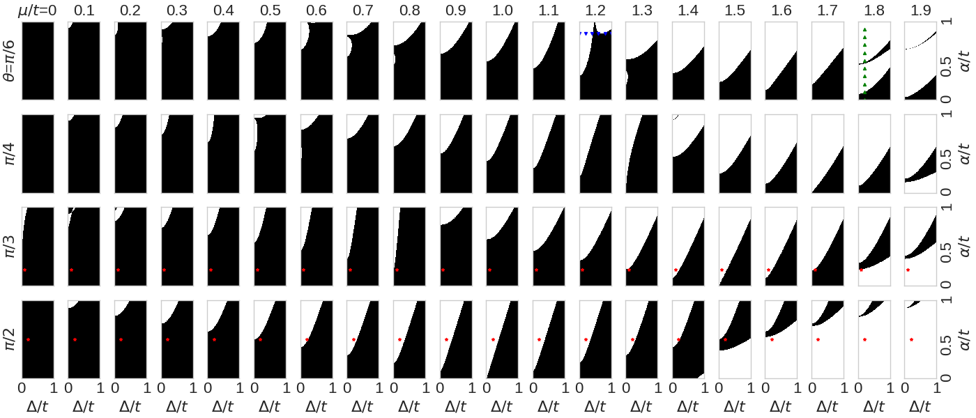
Figure 2: Dependence of $\mathbb{Z}_{2}$ topological invariant on chemical potential ($\mu$), SC gap ($\Delta$), and RSOC ($\alpha$) and spiral spinon texture with phase modulation angle $\theta$. The topologically trivial (non-trivial) phase is shown in white (black). In the figure the columns represent the chemical potential $\mu/t$ (increasing from left to right). The rows represent the phase of the spinon texture $\theta=\pi/6,\pi/4,\pi/3,\pi/2$. $x$-axis of each sub-figure represents the SC gap $\Delta/t\in\left(0,1\right)$ and y-axis represent the RSOC $\alpha/t\in\left(0,1\right)$. For $\theta=\pi/2$ (last row, $\alpha/t=0.5$, $\Delta/t=0.2$) and $\theta=\pi/3$ (second last row, $\alpha/t=0.2$, $\Delta/t=0.1$) the points marked by star (red) represent the re-entrant topological transition — from topologically non-trivial (black) to trivial (white), to again non-trivial phase (black) — as $\mu/t$ is varied. The same transition is also shown as $\Delta$ (first row, $\theta=\pi/6,\mu/t=1.2$, blue down-triangle) and $\alpha$ (first row, $\theta=\pi/6,\mu/t=1.8$, green up-triangle) are varied.

The topological invariant $Q$ is related to $A_{k}$, which is a function of parameters $\mu$, $\theta$, $\Delta$ and $\alpha$. Therefore an interesting topological phase diagram can be found by tuning accordingly these parameters. In Fig. 2 we plot the dependence of $Q$ on these parameters, specifically, we plot the topological invariant $Q$ on the $\Delta$–$\alpha$ parameter space for different combination of $\mu$ and $\theta$. It can be observed that at constant $\theta$ (every row) and increasing $\mu$ (from left to right) the area of the topologically non-trivial phase (black) decreases. We also observe that, in each row the trivial phase starts to seep in from higher $\alpha$ and lower $\Delta$ as $\mu/t$ is increased. For example, when $\theta=\pi/6$ (first row) and $\mu/t=0.01$ the whole $\Delta$–$\alpha$ parameter space has a non-trivial topological phase ($Q=-1$, black). When $\mu/t=0.1,0.2$ the trivial phase ($Q=1$, white) starts to seep in from the upper left corner. With a further increase in $\mu/t$ the area of topological phase increases. This can be understood by keeping in mind the energy spectrum of the archetypal Kitaev chain and by observing the momentum space energy spectrum of the Hamiltonian, Eq. (12) [1, 34] . Although Eq. (11) is analogous to the Hamiltonian of the archetypal Kitaev chain in real space, but in momentum space the energy spectrum differs from each other due to presence of $\theta$. Effect of inclusion of $\theta$ in the Hamiltonian are of two folds. First, with the increase in $\theta$ the energy dispersion becomes flatter (hopping is proportional to $t\cos(\theta/2)$, hence the width of band decreases), therefore, the electrons become more localized. Second, when $\alpha\neq 0$, depending on periodicity of $\tilde{t}_{i}$ (periodicity depends on $\theta$) corresponding number of band gaps appear in the energy spectrum; when $\alpha=0$ only a single band is present as $\tilde{t}_{i}$ loses its periodicity. In Fig. 3 we plot the energy spectrum for $\theta=\pi/3$ and $\alpha/t=0.2,0.4,0.6,0.8$. We see that six energy bands are present for each $\alpha$; it was expected as periodicity of $\tilde{t}_{i}$ in this case is sixfold. Besides, we also observe that with the increase in $\alpha$ the energy gap increases, and bands become flatter. Now the reason for the onset of the trivial phase from the values $\alpha\approx 1,\Delta\approx 0$ (upper left corner of each row) in Fig. 2 is clear. At high $\alpha$ the bands are flatter compared to the ones with low $\alpha$. Therefore, when for higher $\alpha$ we gradually increase $\mu$ the maximum of the band is reached first, compared to the lower $\alpha$ case. For example in Fig. 3 when $\alpha/t=0.8$ the $\mu/t=0.5$ level already lies inside the band gap between the first and the second bands (the bands are counted from $\mu/t=0$), whereas, for $\alpha/t=0.2$ it lies inside the first band. Therefore in the Fig. 2 for $\theta=\pi/3$, $\Delta/t\approx 0$ and $\mu/t=0.5$ the system is already in trivial topological phase for $\alpha/t=0.8$, although, for $\alpha/t=0.2$ the topological non-trivial phase is still present in the system.

Another interesting feature we observe in Fig. 2, is the multiple transition from topologically trivial to non-trivial phase (and vice-versa) as the parameters are varied (we call it “re-entrant” topological phase transition). For example the system for $\theta=\pi/3$, $\alpha/t=0.2$, $\Delta/t=0.1$ (red star, second last row in Fig. 2) goes through phase transitions three times as $\mu$ increases: (i) at $\mu/t=1.3$ from non-trivial to trivial phase, (ii) at $\mu/t=1.8$ from trivial to non-trivial phase, (iii) at $\mu/t=1.9$ from non-trivial to trivial phase. This can be qualitatively understood from the energy spectrum diagram of Fig. 3. In Fig. 3 for $\alpha/t=0.2$ three bands are present. As $\mu$ is increased the system goes through all these bands. The transition from non-trivial (trivial) to trivial (non-trivial) phase occurs when $\mu$ goes from inside the band (band gap) into the band gap (band). In the band gap there is not electronic states to generate MFs, hence, the phase is trivial. This is analogous to the behavior of the archetypal Kitaev chain [1]. In Kitaev chain due to absence of the periodicity only single band is present. When the $\mu$ lies inside the band $-2<\mu/t<2$ then non-trivial phase is present. However, when $\mu$ lies outside this range the phase is trivial. In our case due to the periodic nature of the Hamiltonian (when $\alpha>0$) and when the BZ gets folded ($N$ times if periodicity is $N$). It results in the band gap at the boundary of the folded BZ. If the $\mu$ lies in the band gap then the phase is trivial; if the $\mu$ lies inside the band then phase is non-trivial. In fact, not only $\mu$, but also, by varying $\Delta$ (blue down triangles in first row of Fig. 2, $\theta=\pi/6$, $\mu/t=1.2$) and $\alpha$ (green up triangles in first row of Fig. 2, $\theta=\pi/6$, $\mu/t=1.8$) the re-entrant topological phase transition can be achieved.

Figure 3: (Upper plots) The energy spectrum in a reduced BZ for $\theta=\pi/3$. The BZ boundary is at $\pi/6$ as the periodicity of $\tilde{t}_{i}$ is sixfold. Depending on the value of $\alpha$, the $\mu$ may be present inside or outside of the band (in the bandgap), e.g. for $\alpha/t=0.2$ the $\mu/t=0.5$ (dotted, black) level is inside the band, however, it is in the bandgap for $\alpha/t=0.8$. (Lower plots) The $x$-axis represent $\mathbb{Z}_{2}$ topological invariant $Q$, and $y$-axis the chemical potential $\mu/t$ for $\theta=\pi/3$, $\Delta/t=0.01$, and $\alpha/t=0.2,0.4,0.6,0.8$. The $\mu/t=0.5$ (dotted, black) shows the presence (for $Q=-1$) of topological phase at $\alpha/t=0.2,0.4$, and the absence (for $Q=1$) of the topological phase at $\alpha/t=0.6,0.8$.

V Numerical simulation

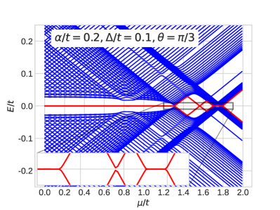
Figure 4: The energy spectrum found by diagonalizing Eq. (11) in the Majorana basis under an open boundary condition for a chain of length $L=100$., $\theta=\pi/3$, $\Delta/t=0.1$ and $\alpha/t=0.2$; these values of the parameters are same as the marked (red, star) position in Fig. 2 for $\pi/3$. (inset) Zoomed portion of energy spectrum around zero energy level from $\mu/t=1.2$ to $1.9$. It is shows that at $\mu/t\approx 1.5$ the MZM really no longer appears.

To make sure that topological phase really occurs in these systems we perform numerical simulations. The signature of a topological phase is the occurrence of two sets of spatially separated odd numbers of MF at two ends of the wire under an open boundary condition; they are represented by MZM states in energy spectrum [34]. In Fig. 4 we numerically diagonalize the Hamiltonian, Eq. (11), under open boundary condition in the Majorana basis. The parameters are same as the marked points in Fig. 2 with $\theta=\pi/3$ (red star). We observe that going from right to left in Fig. 2 at these parameters the system undergoes through three phase transitions. In the numerical simulation in Fig. 4 we also observe these three phase transitions (destruction and creation of zero modes).

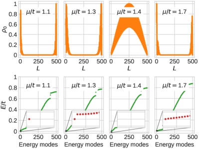
Figure 5: (Upper plots) Normalized LDOS ($\rho_{0}$) of the lowest energy modes along the wire. $\rho_{0}$ is found by diagonalizing (in a Nambu basis) the Hamiltonian, Eq. (11), for a wire of length $L=500$, $\theta=\pi/3$, $\Delta/t=0.2$, $\alpha/t=0.1$. The two peaks at the two ends of the wire for $\mu/t=1.1,1.3,1.7$ shows the presence of spatially separated Majorana fermions. When $\mu/t=1.4$ the Majorana fermions are not localized at the end of the wire, but they can instead be found in the bulk. (Lower plots) The positive energy modes calculated by diagonalizing (in the Majorana basis) the Hamiltonian for the same parameter values. (inset) Shows the presence of zero energy modes for $\mu/t=1.1,1.3,1.7$, and absence of the zero energy modes at $\mu/t=1.4$.

To determine the positions of the zero modes, i.e. whether they really are localized at the end of the wire or not, we numerically diagonalized the real space Hamiltonian (in Nambu basis) of a chain of length $L=500$ and find the localized density of states (LDOS) of the zeroth mode energy ($\rho_{0}$) [36] for $\theta=\pi/3$, $\alpha/t=0.1$, $\Delta/t=0.2$ and $\mu/t=1.1,1.3,1.4,1.7$; in Fig. 2 these parameters are also marked (red star). In Fig. 5 the presence of two peaks at the two ends of the wire is due to localization of the MFs at the two end of the wire for $\mu/t=1.1,1.3,1.7$. However, for $\mu/t=1.4$ the MFs are not localized at the end of the wire and can be found in the bulk of the wire; hence, they are not topologically protected. The same behavior is shown in the analytically calculated phase diagram in Fig. 2. To make sure, that the end states are really MZM, in Fig. 5 (lower plots) we also show the energy modes of the same wire with same parameter configurations. We can clearly observe that the zero modes are present for $\mu/t=1.1,1.3,1.7$ and absent in $\mu/t=1.4$.

VI Dynamic Ground states

Figure 6: In each subfigure the dependence of the free energy on dynamical parameter $\theta$ (x-axis) and external parameter $\mu$ (y-axis) is shown. The values of other parameters $\alpha/t$ (column wise, top heading, left to right) and $\Delta/t$ (row wise, right heading, top to bottom) varies in the region $0.1<\alpha/t,\Delta/t<0.7$. The topologically trivial regions is marked by crosses ($\bm{\times}$). The free energy is shown only for topologically non-trivial regions. The bold black line represent the evolution of the $\theta$ corresponding to the minimum free energy as $0<\mu/t<2$ is varied. If the minimum free energy $\theta$ (bold black line) has values away from $\theta\approx 0,\pi$ and outside the topologically trivial region then the system is in topologically non-trivial state.

In the investigated Hamiltonian, Eq. (11), $\alpha$, $\Delta$, $\mu$ and $\theta$ define the existing topological properties. Among these parameters $\mu$ is the easiest to tune in experimental setup (through the variation of the gate voltage). $\alpha$ and $\Delta$ are the material parameters, which are hard to tune experimentally. $\theta$ is the dynamic parameter (in the absence of an external modulating field), which depends on the value of other parameters of the system; it should take the value to decrease the free energy of the system. With these considerations, it is interesting to investigate: (i) how $\theta$ (for fixed $\alpha$ and $\Delta$) dynamically reacts to a change in $\mu$; (ii) can the tuning of $\mu$ be used to drive the system into and out of the topologically non-trivial phase?

To answer these questions, we numerically calculate the dependence of the free energy on all the parameters of the system. this is done by diagonalizing and integrating the Hamiltonian, Eq. (12), over the whole BZ; it should be kept in mind that for a non-zero $\alpha$ the BZ gets folded $N=2\pi/\theta$ times (the periodicity of the lattice). In Fig. 6 we plot the dependence of the free energy on the dynamic parameter $\theta$ and on the external parameter $\mu$ for different combinations of $0<\alpha/t<0.7$ and $0<\Delta/t<0.7$. The region ($\theta$–$\mu$ parameter space) where the topologically non-trivial phase occurs, the free energy is shown by color gradients; the region where trivial topological phase occurs, the free energy is not shown, and marked by crosses ($\bm{\times}$). The phase is topologically non-trivial if the following two conditions are satisfied: (i) $\theta$ should not have the value of $0<\theta<\pi$ (loosely $\theta\not\approx 0,\pi$), (ii) the $\mathbb{Z}_{2}$ topological invariant should be $Q=-1$. In Fig. 6 we also show the values of $\theta$ corresponding to the minimum free energy ($\theta_{\text{min}}$, bold black line). The answer to the question, whether or not it is possible to use $\mu$ for driving the system into or out of the topologically non-trivial phase, is affirmative, provided the following conditions are satisfied. First, $\theta_{\text{min}}$ lies in the region where the aforementioned topological conditions are satisfied. Second, a non-stringent condition, $\theta_{\text{min}}$ does not lie in the vicinity of the boundary of the topological and trivial phase. This latter condition is added to make sure that a small perturbation of the system should not affect the topological properties . For example, at $\alpha/t=0.1$, $\Delta/t=0.1$, and $0<\mu/t\lessapprox 1$ the $\theta_{\text{min}}\approx\pi$, hence, the system is in a trivial phase. For $1\lessapprox\mu/t\lessapprox 1.4$ the $\theta_{\text{min}}\not\approx 0,\pi$, and inside the region where topological conditions are satisfied, the system is in a topological phase. However, for $\mu/t\gtrapprox 1.4$ the $\theta_{\text{min.}}$ is at the boundary of both a trivial and a non-trivial topological phase, and we can no longer guarantee the stability of such topological phase.

One of the peculiar things in these figures is the presence of topologically non-trivial islands inside the trivial phase, e.g. for $\Delta/t=0.1$ and $\alpha/t=0.7$ such topological phase is present when $\pi/8\lessapprox\theta\lessapprox\pi/2$ and $0.2\lessapprox\mu/t\lessapprox 1$. This happens due to the re-entrant nature of the topological phase.

VII Proposal for experimental realization

To observe the predicted effect three ingredients are necessary: (i) a 1D electronic channel with an extended s-wave superconducting order parameter and non-zero RSOC, (ii) a mechanism to tune chemical potential, (iii) a mechanism to detect MFs. One of the possible way for satisfying the first requirement is to use the heterostructures involving Moire lattices; the schematic is shown in Fig. 1b. Several parallel (Quasi-)1D Moire patterns (electronic channels) on a 2D layered vdW materials can be produced by stretching or straining [38, 39, 40]. To generate Moire patterns multiple layers of vdW materials with strong e-e correlation can be used [22, 41, 42]. Single electronic channels can be isolated by cutting parallel 1D Moire patterns by lasers or atomic force microscope (see [43] and references therein). We assume that the electronic channels are long enough so that electronic state quantization along the length can be ignored, and thin enough that the 1D sub-bands are well separated on the relevant energy scale. To induce extended s-wave superconductivity in these isolated electronic channels one can use iron-based SC, e.g. Fe(Se,Te), Pr doped CaFe₂As₂ ($T_{c}\approx 49$K [44]), or oxyarsenide Sm[O_1-xF_x]FeAs ($T_{c}\approx 55$K [45]). A proximity induced superconductivity has been confirmed in Fe(Se,Te) (see references within [[][]zhu-2023-proxim-effec]). Second requirement is satisfied through gate voltage; by varying the gate voltage one can tune the chemical potential. In Fig. 1b super gate satisfy this function.

The third requirement can be satisfied by biasing the 1D channel and measuring differential conductivity (dI/dV). Back gates (blue gates in Fig. 1) are used to for biasing the electronic channel. Tunnel gates (pink gates) are used to induced tunnel potential; it is needed to control the electron flow. The tunneling spectroscopy is found by measuring dI/dV increasing the back gate bias voltage ($V$) from $-V_{0}$ to $+V_{0}$ at constant tunnel gate voltage and super gate voltage. We expect a peak in dI/dV in the presence of MF.

Recently it was predicted that in depleted InAs NW e-e correlation is strong [20]. Hence, the already available heterostructures involving InAs [4], can also be used for the investigation of MF in a strong correlation regime (without an external magnetic field), the only difference there is the presence of an extra gate to deplete InAs NW and absence of the magnetic field.

The presence of the zero bias dI/dV peak does not always mean emergence of the MF. The zero bias peak can also appear due to Andreev bound states [47]. Hence, several other non-local MF detection methods are also proposed [48]. The proposed heterostructure can be modified accordingly for non-local detection of the MF.

VIII Conclusion

In this work we systematically investigated the effect of the RSOC on the topological properties of the 1D nanowire in the e-e strong correlation regime. The strong e-e correlation allows for the fractionalization of the charge (holon) and spin (spinon) degrees of freedom, which we treat using the su(2|1) path integral method. The resulting Hamiltonian in the presence of spiral spinon field (with modulation angle $\theta$) is given in Eq. (11). It should be stressed that $\theta$ is a dynamic parameter (in the absence of external modulation field), and depends on spinon degree of freedom ($z_{i}$) — $\theta$ is related to $z_{i}$ through Eqs. (9) and (5). We find that for a minimal setup the magnetic field and RSOC are not necessary for topological phase to appear, provided e-e correlation is strong enough. When $0<\alpha$ and $0<\theta<\pi$ by tuning $\mu$ the system can be driven into or out of the topological phase as shown in Fig. 2. It happens because non-zero $\alpha$ induces a quasi period — through periodic electron hopping $\tilde{t}_{i}$, Eq. (11) — in the 1D effective Hamiltonian. It results in folding of the energy dispersion in the BZ and emergence of gaps at folded BZ boundary; explained schematically in Fig. 1a. If the $\mu$ lies inside the energy gap then the topological phase is absent; if $\mu$ lies inside the band then topological present. Schematically it is shown in Fig. 3 for $\theta=\pi/3$. Qualitatively, this situation is same as the original 1D Kitaev toy model [1]. In the Kitaev toy model if the chemical potential lies inside the band ($-2<\mu/t<2$) then topological phase is present, however, if $\mu/t<-2$ or $2<\mu/t$ then the topological phase is absent. The only difference in our case is the occurrence of band gaps due to the folding of the BZ. We numerically validate the re-entrant topological properties as shown in Fig. 4 (Majorana energy spectrum) and Fig. 5 (LDOS of Majorana fermions). In Fig. 6 we calculate the $\theta$ corresponding the minimum free energy for $0<\mu/t<2$. We find that the system can be forced into or out of the topological phase just by tuning $\mu$. We propose heterostructure involving (quasi-)1D Moire structure, shown in Fig. 1b, to investigate the predicted effect.

IX Acknowledgements

K.K.K wish to thank P. A. Maksimov for valuable discussion. K.K.K acknowledges the financial support from the JINR grant for young scientists and specialists, the Foundation for the Advancement of Theoretical Physics and Mathematics ”Basis” for grant # 23-1-4-63-1. One of us, A.F., acknowledges financial support from the MEC, CNPq (Brazil) and from the Simons Foundation (USA).

References

- Kitaev [2001] A. Y. Kitaev, Unpaired Majorana fermions in quantum wires, Physics-Uspekhi 44, 131 (2001).
- Sarma et al. [2015] S. D. Sarma, M. Freedman, and C. Nayak, Majorana zero modes and topological quantum computation, npj Quantum Information 1, 1 (2015).
- Yazdani et al. [2023] A. Yazdani, F. von Oppen, B. I. Halperin, and A. Yacoby, Hunting for majoranas, Science 380, eade0850 (2023).
- Flensberg et al. [2021] K. Flensberg, F. von Oppen, and A. Stern, Engineered platforms for topological superconductivity and majorana zero modes, Nature Reviews Materials 6, 944 (2021).
- Lutchyn et al. [2018] R. M. Lutchyn, E. P. A. M. Bakkers, L. P. Kouwenhoven, P. Krogstrup, C. M. Marcus, and Y. Oreg, Majorana zero modes in superconductor–semiconductor heterostructures, Nature Reviews Materials 3, 52 (2018).
- Mandal et al. [2023] M. Mandal, N. C. Drucker, P. Siriviboon, T. Nguyen, A. Boonkird, T. N. Lamichhane, R. Okabe, A. Chotrattanapituk, and M. Li, Topological superconductors from a materials perspective, Chemistry of Materials 35, 6184 (2023).
- Frolov et al. [2020] S. M. Frolov, M. J. Manfra, and J. D. Sau, Topological superconductivity in hybrid devices, Nature Physics 16, 718 (2020).
- Pawlak et al. [2019] R. Pawlak, S. Hoffman, J. Klinovaja, D. Loss, and E. Meyer, Majorana fermions in magnetic chains, Progress in Particle and Nuclear Physics 107, 1 (2019).
- Fu and Kane [2008] L. Fu and C. L. Kane, Superconducting Proximity Effect and Majorana Fermions at the Surface of a Topological Insulator, Physical Review Letters 100, 096407 (2008).
- Fatemi et al. [2018] V. Fatemi, S. Wu, Y. Cao, L. Bretheau, Q. D. Gibson, K. Watanabe, T. Taniguchi, R. J. Cava, and P. Jarillo-Herrero, Electrically tunable low-density superconductivity in a monolayer topological insulator, Science 362, 926 (2018).
- You et al. [2021] J.-Y. You, B. Gu, G. Su, and Y. P. Feng, Two-dimensional topological superconductivity candidate in a van der waals layered material, Physical Review B 103, 104503 (2021).
- Li et al. [2021] Y. W. Li, H. J. Zheng, Y. Q. Fang, D. Q. Zhang, Y. J. Chen, C. Chen, A. J. Liang, W. J. Shi, D. Pei, L. X. Xu, S. Liu, J. Pan, D. H. Lu, M. Hashimoto, A. Barinov, S. W. Jung, C. Cacho, M. X. Wang, Y. He, L. Fu, H. J. Zhang, F. Q. Huang, L. X. Yang, Z. K. Liu, and Y. L. Chen, Observation of topological superconductivity in a stoichiometric transition metal dichalcogenide 2m-ws2, Nature Communications 12, 2874 (2021).
- Kezilebieke et al. [2022] S. Kezilebieke, V. Vaňo, M. N. Huda, M. Aapro, S. C. Ganguli, P. Liljeroth, and J. L. Lado, Moiré-enabled topological superconductivity, Nano Letters 22, 328 (2022).
- Stoudenmire et al. [2011] E. M. Stoudenmire, J. Alicea, O. A. Starykh, and M. P. Fisher, Interaction effects in topological superconducting wires supporting Majorana fermions, Physical Review B 84, 014503 (2011).
- Aksenov et al. [2020] S. V. Aksenov, A. O. Zlotnikov, and M. S. Shustin, Strong Coulomb interactions in the problem of Majorana modes in a wire of the nontrivial topological class BDI, Physical Review B 101, 125431 (2020).
- Aksenov et al. [2023] S. V. Aksenov, A. D. Fedoseev, M. S. Shustin, and A. O. Zlotnikov, Effect of local coulomb interaction on majorana corner modes: Weak and strong correlation limits, Physical Review B 107, 125401 (2023).
- Zlotnikov et al. [2020] A. O. Zlotnikov, S. V. Aksenov, and M. S. Shustin, Spin-orbit coupling-induced effective interactions in superconducting nanowires in the strong correlation regime, Physics of the Solid State 62, 1612 (2020).
- Kesharpu et al. [2024a] K. K. Kesharpu, E. A. Kochetov, and A. Ferraz, Proposal for realizing majorana fermions without external magnetic field in strongly correlated nanowires, Physical Review B 109, 115140 (2024a).
- Giamarchi [2004] T. Giamarchi, Quantum Physics in One Dimension, The International Series of Monographs on Physics No. 121 (Clarendon ; Oxford University Press, Oxford : New York, 2004).
- Sato et al. [2019] Y. Sato, S. Matsuo, C.-H. Hsu, P. Stano, K. Ueda, Y. Takeshige, H. Kamata, J. S. Lee, B. Shojaei, K. Wickramasinghe, J. Shabani, C. Palmstrøm, Y. Tokura, D. Loss, and S. Tarucha, Strong electron-electron interactions of a tomonaga-luttinger liquid observed in inas quantum wires, Physical Review B 99, 155304 (2019), shows that strong interaction can be induced by gate tuning.
- Kim et al. [2020] M. Kim, S. G. Xu, A. I. Berdyugin, A. Principi, S. Slizovskiy, N. Xin, P. Kumaravadivel, W. Kuang, M. Hamer, R. K. Kumar, R. V. Gorbachev, K. Watanabe, T. Taniguchi, I. V. Grigorieva, V. I. Fal’ko, M. Polini, and A. K. Geim, Control of electron-electron interaction in graphene by proximity screening, Nature Communications 11, 2339 (2020).
- Balents et al. [2020] L. Balents, C. R. Dean, D. K. Efetov, and A. F. Young, Superconductivity and strong correlations in moiré flat bands, Nature Physics 16, 725 (2020).
- Hosono et al. [2018] H. Hosono, A. Yamamoto, H. Hiramatsu, and Y. Ma, Recent advances in iron-based superconductors toward applications, Materials Today 21, 278 (2018).
- Ferraz and Kochetov [2011] A. Ferraz and E. A. Kochetov, Effective action for strongly correlated electron systems, Nuclear Physics B 853, 710 (2011).
- Ferraz and Kochetov [2022] A. Ferraz and E. Kochetov, Fractionalization of strongly correlated electrons as a possible route to quantum Hall effect without magnetic field, Physical Review B 105, 245128 (2022).
- Kesharpu [2024] K. K. Kesharpu, Topological Hall effect in strongly correlated layered magnets: The effect of the spin of the magnetic atoms and of the polar and azimuthal angles subtended by the spin texture, Physical Review B 109, 205120 (2024).
- Kesharpu et al. [2023] K. K. Kesharpu, E. A. Kochetov, and A. Ferraz, Topological Hall effect induced by classical large-spin background: $su(2)$ path-integral approach, Physical Review B 107, 155146 (2023).
- Ferraz and Kochetov [2023] A. Ferraz and E. Kochetov, Connection between the Kitaev chain and the Gutzwiller-projected BCS model, Annals of Physics 456, 169234 (2023).
- Kesharpu et al. [2024b] K. K. Kesharpu, E. A. Kochetov, and A. Ferraz, Treatment of the strongly correlated topological superconductors through the path-integral technique, arXiv:2407.07022 [cond-mat.str-el] (2024b).
- Note [1] Substituting Eq. (8) in Eq. (6) or Eq. (7) will give .
- Note [2] For AFM case , which also results in .
- Ryu et al. [2010] S. Ryu, A. P. Schnyder, A. Furusaki, and A. W. W. Ludwig, Topological insulators and superconductors: Tenfold way and dimensional hierarchy, New Journal of Physics 12, 065010 (2010).
- Tewari and Sau [2012] S. Tewari and J. D. Sau, Topological invariants for spin-orbit coupled superconductor nanowires, Physical Review Letters 109, 150408 (2012).
- Alicea [2012] J. Alicea, New directions in the pursuit of Majorana fermions in solid state systems, Reports on Progress in Physics 75, 076501 (2012).
- Note [3] For an archetypal Kitaev chain the energy spectrum as a cosine dependence [34]. The topological boundary corresponds to ; physically it corresponds to the maximum () and minimum () of the energy band.
- Sacramento et al. [2007] P. D. Sacramento, V. K. Dugaev, and V. R. Vieira, Magnetic impurities in a superconductor: Effect of domain walls and interference, Physical Review B 76, 014512 (2007).
- Note [4] Although, by definition the topological properties of the system should not be prone to perturbation, however, here we are talking about the perturbation around the limiting values of the parameters.
- Dróżdż et al. [2024] P. Dróżdż, M. Gołębiowski, and R. Zdyb, Quasi-1d moiré superlattices in self-twisted two-allotropic antimonene heterostructures, Nanoscale 16, 15960 (2024).
- Sinner et al. [2023] A. Sinner, P. A. Pantaleón, and F. Guinea, Strain-induced quasi-1d channels in twisted moiré lattices, Physical Review Letters 131, 166402 (2023).
- Santos and Dias [2021] F. D. R. Santos and R. G. Dias, Superconductivity in twisted bilayer quasi-one-dimensional systems with flat bands, Physical Review B 104, 165130 (2021).
- Liu and Yu [2023] S. Liu and G. Yu, Fabrication, energy band engineering, and strong correlations of two-dimensional van der waals moiré superlattices, Nano Today 50, 101829 (2023).
- Checkelsky et al. [2024] J. G. Checkelsky, B. A. Bernevig, P. Coleman, Q. Si, and S. Paschen, Flat bands, strange metals and the kondo effect, Nature Reviews Materials 9, 509 (2024).
- Lau et al. [2022] C. N. Lau, M. W. Bockrath, K. F. Mak, and F. Zhang, Reproducibility in the fabrication and physics of moiré materials, Nature 602, 41 (2022).
- Lv et al. [2011] B. Lv, L. Deng, M. Gooch, F. Wei, Y. Sun, J. K. Meen, Y.-Y. Xue, B. Lorenz, and C.-W. Chu, Unusual superconducting state at 49 k in electron-doped cafe <sub>2</sub> as <sub>2</sub> at ambient pressure, Proceedings of the National Academy of Sciences 108, 15705 (2011), iron based superconductor wiht highest Tc at ambient pressure.
- Zhi-An et al. [2008] R. Zhi-An, L. Wei, Y. Jie, Y. Wei, S. Xiao-Li, Zheng-Cai, C. Guang-Can, D. Xiao-Li, S. Li-Ling, Z. Fang, and Z. Zhong-Xian, Superconductivity at 55 k in iron-based f-doped layered quaternary compound sm[o <sub> 1- <i>x</i> </sub> f <sub> <i>x</i> </sub> ] feas, Chinese Physics Letters 25, 2215 (2008).
- Zhu and Zhou [2023] Q.-G. Zhu and T. Zhou, Proximity effect and inverse proximity effect in a topological-insulator/iron-based-superconductor heterostructure, Physical Review B 107, 094506 (2023).
- Prada et al. [2020] E. Prada, P. San-Jose, M. W. A. De Moor, A. Geresdi, E. J. H. Lee, J. Klinovaja, D. Loss, J. Nygård, R. Aguado, and L. P. Kouwenhoven, From Andreev to Majorana bound states in hybrid superconductor–semiconductor nanowires, Nature Reviews Physics 2, 575 (2020).
- Zhang et al. [2019] H. Zhang, D. E. Liu, M. Wimmer, and L. P. Kouwenhoven, Next steps of quantum transport in Majorana nanowire devices, Nature Communications 10, 5128 (2019).