Predicting ionic conductivity in solids from the machine-learned potential energy landscape

Abstract

Discovering new superionic materials is essential for advancing solid-state batteries, which offer improved energy density and safety compared to the traditional lithium-ion batteries with liquid electrolytes. Conventional computational methods for identifying such materials are resource-intensive and not easily scalable. Recently, universal interatomic potential models have been developed using equivariant graph neural networks. These models are trained on extensive datasets of first-principles force and energy calculations. One can achieve significant computational advantages by leveraging them as the foundation for traditional methods of assessing the ionic conductivity, such as molecular dynamics or nudged elastic band techniques. However, the generalization error from model inference on diverse atomic structures arising in such calculations can compromise the reliability of the results. In this work, we propose an approach for the quick and reliable evaluation of ionic conductivity through the analysis of a universal interatomic potential. Our method incorporates a set of heuristic structure descriptors that effectively employ the rich knowledge of the underlying model while requiring minimal generalization capabilities. Using our descriptors, we rank lithium-containing materials in the Materials Project database according to their expected ionic conductivity. Eight out of the ten highest-ranked materials are confirmed to be superionic at room temperature in first-principles calculations. Notably, our method achieves a speed-up factor of approximately 50 compared to molecular dynamics driven by a machine-learning potential, and is at least 3,000 times faster compared to first-principles molecular dynamics.

I Introduction

Solid-state batteries (SSBs) are a promising alternative to traditional lithium-ion batteries due to their higher energy density and enhanced safety features. With the elimination of liquid electrolytes, SSBs reduce the risk of leakage and combustion, thus mitigating one of the major safety concerns with conventional batteries [1, 2, 3]. Coupled with the potential for increased energy storage [4], this safety enhancement makes SSBs a crucial technology for advancing electric vehicles and portable electronics, where the demand for longer battery life and robust performance is ever-increasing.

Despite these advantages, SSBs development faces a number of challenges that prevents their widespread adoption [5]. One major limitation is the relatively low ionic conductivity of solid electrolytes compared to their liquid counterparts, which can diminish the overall performance of the battery. Additionally, interface stability between the solid electrolyte and electrodes remains a critical issue [6, 7]. The formation of interfacial resistance and degradation over time can significantly impact the lifespan and efficiency of a battery [6]. Therefore, there is a pressing need for the development of new solid-state electrolytes (SSEs) with improved properties to overcome these barriers.

To address these challenges, computational prediction methods have been employed to identify and optimize new SSE materials [8, 9, 10, 11, 12]. However, these methods are often computationally expensive and time-consuming. Machine learning (ML) presents a viable solution to mitigate these limitations [13, 14, 15, 16, 17, 18, 19, 20, 21, 22, 23, 24]. By leveraging large datasets such as the Materials Project database [25] and advanced algorithms, ML has the potential to speed up the discovery of new materials with high ionic conductivity and therefore accelerate the research and development of high-performance SSBs [26, 27].

Different ML algorithms that have been employed to assist the discovery of superionic materials include classical supervised ML methods like logistic regression [28, 29], gradient boosting [30] and support vector machines [31, 32], classical unsupervised methods [33, 26], as well as deep learning approaches based on graph neural networks (GNN) [34, 35, 36]. The main difficulty in implementing the ML models for identifying SSEs is in general the limited availability of high-quality data on ionic mobility in solids. This motivates the use of knowledge transfer methods [32], or trading off for larger datasets [35] obtained using approximate methods [37].

The scarcity of available data drives the search for informative material descriptors that correlate well with ionic conductivity. This search is typically focused on descriptors that characterize compositions, geometric configurations, and electrochemical and electronic properties of materials [38, 26, 39], often relying on implementations from the matminer library [40], which are adapted from scientific publications. In this work, we aim to expand this focus by exploring the features of the interatomic potential (IAP).

While IAP can be evaluated with expensive first-principles density functional theory (DFT) calculations, ML models allow for bypassing this step. Since there is notably more high-quality data available for predicting interatomic forces and energies, the task of predicting IAP is far less constrained than identifying SSEs directly. In fact, various ML methods have been proposed in the past decades to effectively bypass DFT in IAP calculations [41, 42, 43].

A notable improvement in the performance and reliability of these methods has been observed after the adoption of graph neural networks (GNNs) [13, 14, 15]. These models inherently impose permutation invariance by operating on graph structures, where the order of nodes does not affect the computation of graph-level representations. Additionally, invariance under 3D translations and rotations is achieved through the use of equivariant message passing and invariant feature aggregation methods. Although most of the initial models utilize 2-body messages, the introduction of many-body messages and updates allowed models like CHGNet [17], M3GNet [16], MACE [18, 19, 20] and the NequIP-based [44] SevenNet [45] achieve significant quality improvement, as demonstrated on the Matbench Discovery public benchmark [46]. These models may also be called universal potentials, as they cover the majority of the elements in the periodic table that are highly relevant to applications.

In the context of ionic transport studies, ML-IAPs can serve as substitutes for DFT in MD [36] and nudged elastic band (NEB) calculations [47]. However, a notable concern with ML-IAPs is the generalization error, which refers to the error in the model’s predictions when applied to new data, unseen at training time. Naturally, one should expect this error to increase as MD and NEB simulations drive the studied systems further from the domain of the training set, leading to a decrease in the model’s predictive accuracy and reliability. A typical way of addressing this issue is through active learning [48, 49]. This involves controlling the prediction error, running DFT on configurations where the error is excessively large and then retraining the model on these configurations. While this approach effectively reduces the generalization error, it sacrifices some of the computational efficiency gained by switching from DFT to ML-IAPs.

In this work, we take a different approach by utilizing a universal potential model to design a set of dedicated descriptors that predict materials with high lithium mobility while minimizing generalization error. We leverage an ML-IAP trained on vast amounts of data to analyze the potential landscape in a controlled environment for the labeled structures present in high-quality computational and experimental Li conductivity datasets. From this analysis, we propose a set of heuristics that can be calculated on structure configurations that are similar to the examples used for training the potential. This ensures minimal generalization requirements for the model and therefore more accurate predictions of the interatomic potential in the diverse material environments. Finally, we use these descriptors to predict SSEs within the Materials Project database and validate our predictions with ab initio calculations.

The studies performed in this work are done using the M3GNet model, which was trained by the authors of the original work [16] on the entire Materials Project dataset [25]. It should be noted, however, that our approach is not specific to a particular model and could be used with any IAP.

This document is structured as follows: Sec. II describes the methodology used throughout this work, outlining the key ideas of the proposed approach in Secs. II.1 and II.2, along with details of the ab initio calculations presented in Sec. II.3. In Sec. III, we report and discuss our findings and provide an outlook. Finally, we conclude in Sec. IV.

II Methodology

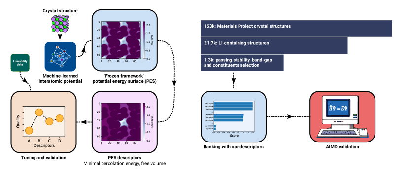
Figure 1: Flowchart of the logical steps performed in our study

The overall computational pipeline performed in this work is shown in Fig. 1. We start from a machine-learned interatomic potential, which is used to analyze the potential energy surface (PES) for a given material. Then, a set of scalar heuristics is derived from the obtained PES. These descriptors are based on our intuition of which PES properties should correlate well with ionic mobility. We further validate our choice and evaluate the quality of the derived heuristics with labeled data, both simulated and experimental. Descriptors that demonstrate robustness and highest predictive power are chosen to rank the structures from the Materials Project dataset [25]. Finally, we perform computationally demanding ab initio molecular dynamics (AIMD) simulation to validate the candidates that are most promising according to our method. We describe our pipeline in greater detail throughout Secs. II.1, II.2 and II.3.

II.1 Potential energy surface in the frozen framework approximation

In this work, we leverage the assumption that the generalization error of the ML-IAP model is reduced when the system under study differs from the closest training object by only the coordinates of a single atom, compared to a system where all the atomic positions differ from those in the training set. Therefore, each structure is considered as having a single mobile ion per unit cell and a frozen framework formed by the remaining atoms. A potential energy surface (PES) scan is performed by placing the mobile ion at a set of locations on a regular 3d grid and evaluating the potential energy for the resulting structure. The grid spans over the entire unit cell with axes parallel to the lattice vectors. For each lattice vector $\vec{l}_{i}$, the grid step along that direction is $\vec{g}_{i}=\vec{l}_{i}/N_{i}$, where $N_{i}$ is the smallest integer satisfying $|\vec{l}_{i}|/N_{i}\leq 0.25$ Å. Locations that are closer than $R_{\text{min}}=1.2$ Å to any of the other atoms are excluded from this process to avoid ML-IAP evaluations on unphysical configurations.

Once the PES values on the grid are obtained, we repeat them along each axis to create a $2\times 2\times 2$ supercell. We position the origin of the grid so that the ion’s lowest energy location is at the center of the supercell, with its 26 replicas located at the outer faces. In other words, the resulting PES is a 3-dimensional array with values corresponding to the mobile ion locations $\vec{r}=\sum_{i}(o_{i}+c_{i})\cdot\vec{g}_{i}$, with $i\in\{1,2,3\}$, $o_{i}$ being the grid coordinates for the minimal PES value and $c_{i}\in\{-N_{i},\ldots,N_{i}\}$. Then, a breadth-first search is performed for a minimum-energy-barrier path from the center to any of the faces of the supercell. Minimal percolation energy (MPE) for this ion is reported as the energy barrier value for the discovered path.

Due to the frozen framework approximation, MPE values are expected to be much larger than the actual activation energies. In reality, ionic hopping in superionic conductors occurs in a timescale of ns [50, 51], which allows for relaxation of the remaining ions and reduces the activation energies. However, our expectation is that MPE reflects the strength of the interactions that are overcome during ionic hopping, and thus correlates with the ionic mobility.

The breadth-first search of the optimal path requires calculating a quantity, which we denote as the level map (LM), given by:

$$\text{LM}(\vec{r})\equiv\underset{C\in\mathscr{C}(\vec{r},\vec{r}_{0})}{\min}\left[\underset{{\vec{r}\,}^{\prime}\in C}{\max}E({\vec{r}\,}^{\prime})\right],$$ (1)

where $\vec{r}_{0}$ is the initial location of the mobile atom at the relaxed state, $\mathscr{C}(\vec{r},\vec{r}_{0})$ is the set of all paths connecting $\vec{r}$ and $\vec{r}_{0}$, and $E({\vec{r}\,}^{\prime})$ is PES value at ${\vec{r}\,}^{\prime}$. The meaning of LM is the minimal amount of energy an ion needs to be able to get to $\vec{r}$ from its original site, within the frozen framework approximation. In our calculation, as explained above, the $\min$ and $\max$ operations are performed on a discrete grid. Using the level map concept, MPE can be defined as:

$$\text{MPE}\equiv\underset{\vec{r}\in\mathscr{F}}{\min}\left[\text{LM}(\vec{r})\right],$$ (2)

where $\mathscr{F}$ denotes the set of points located at the faces of the supercell, where the replicas of the original site are located.

Finally, we introduce another family of structure characteristics that we call free volumes (FV) by calculating the average volume of PES/LM below a certain threshold $t$:

$$\text{FV}_{X}(t)=\frac{1}{V}\int\limits_{\text{supercell}}\mathds{1}\left[X\vphantom{{}^{0}_{0}}(\vec{r})<t\right]d\vec{r},$$ (3)

where $V$ denotes the full volume of the supercell, $\mathds{1}[\cdot]$ is the indicator function and $X(\vec{r})$ can be either $E(\vec{r})$ or $\text{LM}(\vec{r})$, in which case the corresponding FV is called disconnected or connected, respectively. This naming choice reflects that, by the definition of LM, any set of points satisfying $\text{LM}(\vec{r})<T$ is a connected set, while this may not necessarily hold for $E(\vec{r})$.

Since a unit cell may contain more than one potentially mobile atom, aggregation is performed over atoms of the mobile species. For the case of MPE, the aggregation operation is just the minimum value of individual MPEs over the mobile atoms. For FVs, the aggregation is done by superimposing the indicator function outputs for different mobile atoms and combining them with logical OR operation prior to volume calculation.

In order to illustrate the way our method is intended to differentiate between good and bad ionic conductors, Fig. 2 shows the $\text{LM}(\vec{r})=0.5$ eV isosurfaces on top of two high-FV, one intermediate-FV and one low-FV structures. Within the frozen framework approximation, these isosurfaces highlight the regions accessible to the central Li atom of each structure under the given energy threshold. We expect the sizes of these regions, and hence their volumes, to correlate with Li mobility in a given material. While the threshold of 0.5 eV may seem extremely high, one should anticipate that the more accurate but expensive PES calculation with framework relaxation would have resulted in much lower LM values.

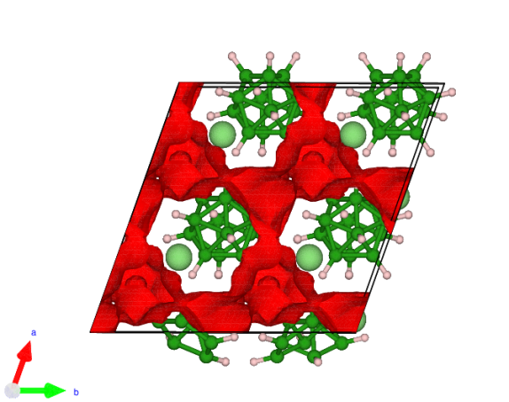
(a) Li(BH)₆

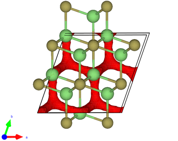
(b) Li₂Te

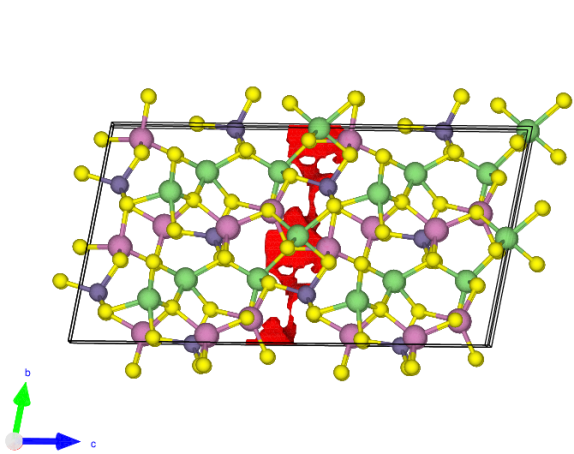
(c) Li₂In₂GeS₆

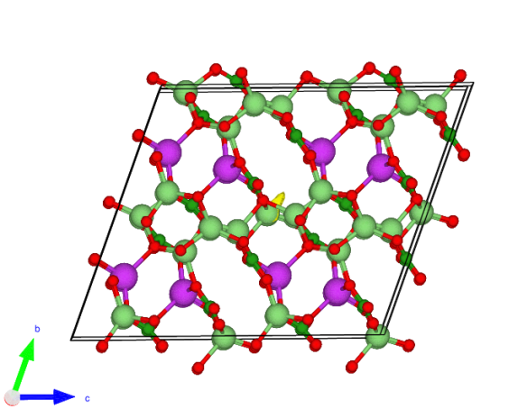
(d) Li₃Bi(BO₃)₂

Figure 2: Level map isosurfaces at the threshold of 0.5 eV. The corresponding structure compositions, Materials Project identifiers and values of the combined $\Xi$ descriptor defined in Sec. II.2 (rounded to two digits) are: LABEL:sub@fig:vesta:mp-1211296 Li(BH)₆ – mp-1211296 – 0.99, LABEL:sub@fig:vesta:mp-2530 Li₂Te – mp-2530 – 0.97, LABEL:sub@fig:vesta:mp-1191476 Li₂In₂GeS₆ – mp-1191476 – 0.35, and LABEL:sub@fig:vesta:mp-768738 Li₃Bi(BO₃)₂ – mp-768738 – 0.00. The isosurfaces are shown in red everywhere except LABEL:sub@fig:vesta:mp-768738, where yellow color is used for the isosurface and red is reserved to denote the oxygen atoms. The structures and isosurfaces are visualized using the VESTA software [52].

II.2 Validating PES descriptors

In order to evaluate our PES descriptors, we make use of two publicly available datasets related to lithium mobility and conductivity. The first dataset, Kahle2020, from the study by L. Kahle et al. [10], includes high-throughput AIMD simulation of lithium diffusivity for 121 materials at 1000 K, with 25 of these materials also simulated at temperatures as low as 500 K. The second dataset, Laskowski2023, is compiled by F. Laskowski et al. [26] in their study focused on identifying promising ionic conductors with a semi-supervised machine learning approach. The dataset consists of experimental conductivities from the literature, measured at or extrapolated to room temperature. It has 334 structures linked to the Inorganic Crystal Structure Database (ICSD) [53], 75 of which can also be successfully associated with entries from the Materials Project. To maximize the utility of the limited data, we ensure that our PES descriptors can highlight good ionic conductors in both the simulated and experimental datasets simultaneously. While our ultimate goal is to predict room-temperature superionic conductors, the prevalence of high-temperature labeled structures in the Kahle2020 dataset is expected to improve our method’s high-temperature predictions, which is still relevant for the mentioned ultimate goal.

The evaluation procedure is set up as follows. Firstly, since the Kahle2020 dataset labels the structures with diffusion coefficients, we convert them to conductivity values via the Nernst-Einstein relation. We also extrapolate the conductivities to room temperature for those structures in Kahle2020 where such extrapolation is possible. We then introduce two conductivity thresholds, $\sigma^{+}$ and $\sigma^{-}$, to label the structures with the conductivity above $\sigma^{+}$ (below $\sigma^{-}$) as good (bad) conductors. We smooth these labels with the assumption of Gaussian error distribution for the given conductivity values. That is, we weight the samples according to the value of the integral above $\sigma^{+}$ (below $\sigma^{-}$) for a Gaussian distribution with mean and standard deviation set to the given conductivity value and its uncertainty.

These labels and weights are then used to calculate ranking scores for each descriptor. Our scoring function is a modification of the commonly used area under the ROC-curve that only considers the lowest 10% of the false-positive rates instead of the full integral. This ensures that we aim towards maximal purity at the top of the list of structures and ignore the order in the lower portion of the list when using our descriptors for ranking potential ionic conductors. The resulting score values for the MPE descriptor and FV descriptors at different energy thresholds are shown in Fig. 3.

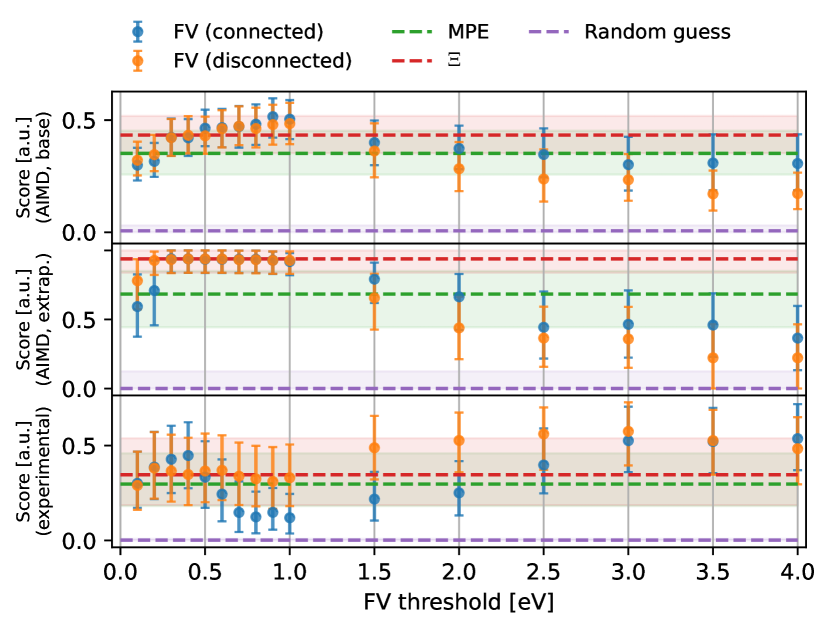
Figure 3: Descriptor evaluation scores. The top panel shows the scores obtained with $T=1000$ K labels from the Kahle2020 dataset. Scores obtained from that dataset with the alternative procedure, when positive classes are defined by the room-temperature-extrapolated conductivity values, are shown in the middle panel. The bottom panel contains the scores resulting from the experimentally measured conductivity labels reported at room temperature in the Laskowski2023 dataset. The top-performing FV descriptors, based on all three evaluation scores, are combined into the SSE-ranking descriptor $\Xi$ (see text) with its performance indicated by the dashed red line. For the reference, a random guess classifier performance is also shown (dashed purple line). The uncertainties are estimated with bootstrapping.

As most of the structures from the Kahle2020 dataset are only simulated at $T=1000$ K, we use the labels at that temperature throughout the dataset to obtain the scores shown in the top panel of Fig. 3, with thresholds set to $\sigma^{+}=0.1$ S / cm and $\sigma^{-}=0.01$ S / cm. In addition, we perform a separate evaluation, shown in the middle panel of Fig. 3, using the room-temperature-extrapolated conductivities when determining the positive classes with $\sigma^{+}\approx 3.16$ mS / cm (the exact relation being defined in log scale as $\log_{10}\left(\sigma^{+}[\text{{S\,/\,cm}}]\right)=-2.5$). For the Laskowski2023 dataset, where all the experimental conductivity values are given at room temperature, we set the thresholds to $\sigma^{+}=0.05$ mS / cm and $\sigma^{-}=0.01$ mS / cm, resulting in the scores shown in the bottom panel of Fig. 3. As uncertainty values are not provided, we use an overestimate of 100% relative uncertainty in our weighting procedure. This, along with a lower conductivity threshold compared to that used in the simulated data analysis, is intended to smooth out the labels for intermediate-quality conductors.

One can see from Fig. 3 that all the proposed descriptors are capable of predicting ionic conductors to some degree, in the sense that they all have scores higher than a random guess. It can also be noted that FV descriptors at thresholds of $0.3-0.5$ eV demonstrate better or equal performance compared to MPE across all the three scores, while there is no particular winner between the connected and disconnected versions of FV. For that reason, we pick both versions of FV at the threshold of 0.5 eV to be further used for ranking the structures with unknown conductivities. We construct a combination of the two descriptors into the SSE-ranking descriptor, denoted as $\Xi$, by simultaneously thresholding them with a sigmoid function:

$$\begin{gathered}\Xi=S_{1}\cdot S_{2},\\ S_{1}=s_{10}\left[2.00+\log_{10}\text{FV}^{\text{connected}}_{0.5\,\text{eV}}\right],\\ S_{2}=s_{10}\left[1.15+\log_{10}\text{FV}^{\text{disconnected}}_{0.5\,\text{eV}}\right],\\ s_{10}(x)\equiv\frac{1}{1+e^{-10x}}.\end{gathered}$$ (4)

The threshold values of $-2.00$ and $-1.15$ for the base-10 logarithms of the connected and disconnected FV values, respectively, were picked to simultaneously discard the low-conductivity entries in both simulated and experimental data, as observed in Figs. 7 and 8 from Appendix B. The performance scores for the resulting $\Xi$ descriptor is also shown in Fig. 3. Alternative ways of combining our descriptors for ranking are discussed in Appendix C.

The combined descriptor is then used to rank the Materials Project structures. We start by querying lithium containing structures with band gap of at least 0.5 eV and energy above hull of at most 0.05 eV / atom, which results in 5997 potential structures. By further discarding the entries containing transition metals we end up with 1302 structures, with 113 of them satisfying $\Xi>0.25$, i.e. being above the two FV thresholds simultaneously. We then perform AIMD validation for the five of these structures with the largest $\Xi$ values. Technical details for these simulations are given in Sec. II.3, while the results are presented in Sec. III.

II.3 Ab initio molecular dynamics

Molecular dynamics simulations of selected structures with the highest $\Xi$ values were carried out using the SIESTA code [54]. The forces were calculated using the generalized gradient approximation (GGA) of density functional theory [55], except for molecular solids, for which we used the LMKLL parameterization [56] of the van der Waals functional of Dion et al. [57]. The core electrons are represented by pseudopotentials of the Troullier-Martins scheme [58]. The basis sets for the Kohn-Sham states are linear combinations of numerical atomic orbitals, of the polarized double-zeta type [59, 60].

For each system, the volume relaxation was initially carried out for the primitive unit cell using a conjugate gradient approach, and the Monkhorst and Pack Brillouin zone sampling grid [61] in the Materials Project data entry [25]. A supercell capable of accommodating a sphere with a diameter of at least 6.5 Å was then constructed and the self-consistent calculation of the charge density carried out using the $\Gamma$-point for Brillouin zone sampling. Then, a molecular dynamics calculation for the same system was carried out at constant temperature using a Nosé thermostat [62] and a maximum number of ten self-consistent iterations per time step. The integration time step of 1 fs was used. Additionally, a number of short cross-check AIMD runs with 0.25 and 0.5 fs step sizes were carried out and showed no significant impact on the observed results. The system is initially equilibrated in a $NVT$ ensemble for 5 ps, after which we acquire data for the diffusivity calculation also in the $NVT$ ensemble.

The diffusion coefficient is obtained by assuming three-dimensional Brownian motion with a mean square displacement (MSD) given by

$${\rm MSD}=\langle\left|\vec{r}(t)-\vec{r}(t_{0})\right|^{2}\rangle=6Dt_{0},$$ (5)

where the ensemble average is over all ions. Since sampling trajectories for multiple starting configurations is prohibitive, we have instead split the trajectory into multiple time windows following the methodology used in [10]. We chose the window length of 15 ps and perform the linear fit on MSD from 1 to 15 ps in each window. The uncertainty for the diffusion coefficients is then estimated from the variance of these fit results over independent fits. A comparison of the diffusivity obtained using alternative fitting intervals can be found in Appendix D. The diffusion coefficients are converted to conductivity values using the Nernst-Einstein relation:

$$\sigma=\frac{nq^{2}}{k_{\text{B}}T}D,$$ (6)

where $\sigma$ is the conductivity value, $D$ is the extracted diffusion coefficient, $k_{\text{B}}$ is the Boltzmann constant, $T$ is the absolute temperature, $n$ is the charge carrier concentration, and $q$ is their charge.

We have also carried out tests for the finite system size effects for structure mp-1211296 which contains a comparatively small number of Li per supercell. To enable access to larger supercells and extended simulation times, we employed an ML-IAP (SevenNet) to drive the MD simulations in these tests. The results confirm that using larger supercells enhances the linearity of the MSD dependence. Notably, the diffusion coefficients extracted from the runs with different supercell sizes show consistent agreement within the statistical uncertainties.

III Results and discussion

We have calculated MPE and FV descriptor values, as well as the SSE-ranking descriptor $\Xi$, for the 5997 structures from the Materials Project dataset that satisfy the minimal selection criteria, as discussed at the end of Sec. II.2. These predictions are made public and can be found at [63]. We observe, that the top of the $\Xi$-ranked list is well populated by the structures from the LGPS family of superionic conductors [64], which supports the effectiveness of the proposed approach. For the optimal use of computational resources, we therefore focus our AIMD simulation on the other less-known structures from the top of the $\Xi$-ranked list. Additionally, a single well-known superionic conductor, Li₇P₃S₁₁ [65] is evaluated to validate our methodology. The summary of our findings is presented in Table 1. AIMD validation results are also shown in Fig. 4, where the extracted conductivity values are plotted against $1/T$.

#	MP identifier	Composition	$\Xi$	AIMD results
				$T$ [K]	$\tau$ [ps]	$\sigma$ [S / cm]	$E_{A}$ [meV]
				1000	53.698	$2.6\pm 0.6$
1	mp-1211100	LiB3H8	0.9924	667	50.430	$1.18\pm 0.11$	$99\pm 93$
				500	52.248	$1.6\pm 0.4$
				1000	60.833	$0.9\pm 0.5$
2	mp-1211296	Li(BH)6	0.9898	667	51.756	$0.30\pm 0.15$	$224\pm 19$
				500	51.754	$0.13\pm 0.05$
				1000	57.168	$3.7\pm 0.4$
3	mp-570935	LiI	0.9812	667	24.413	$-0.016^{*}$	NA
				500	66.191	$(2.2\pm 1.0)\times 10^{-3}$
4	mp-721239	Li10Ge(PSe6)2	0.9746	-	-	-	-
5	mp-721252	Li10Sn(PSe6)2	0.9729	-	-	-	-
				1000	41.944	$4.19\pm 0.17$
6	mp-2530	Li2Te	0.9712	667	48.011	$(0.46\pm 0.10)\times 10^{-3}$	NA
				500	47.926	$-(0.5\pm 1.8)\times 10^{-3}$
7	mp-721253	Li10Si(PSe6)2	0.9712	-	-	-	-
8	mp-705516	Li10Sn(PSe6)2	0.9661	-	-	-	-
				1000	65.610	$4.9\pm 0.9$
9	mp-644223	LiBH4	0.9647	667	62.477	$1.4\pm 0.7$	$320\pm 43$
				500	72.662	$0.14\pm 0.16$
10	mp-696127	Li10Ge(PSe6)2	0.9645	-	-	-	-
				1000	69.483	$1.96\pm 0.14$
12	mp-641703	Li7P3S11	0.9606	667	57.364	$0.8\pm 0.2$	$251\pm 15$
				500	59.836	$0.20\pm 0.05$
25	mp-696128	Li10Ge(PS6)2	0.9379	-	-	-	-

Table 1: Top $\Xi$ predictions and AIMD results summary. Ten structures with highest $\Xi$ values are shown. In addition, two known superionic conductors, Li₇P₃S₁₁ [65] and Li₁₀Ge(PS₆)₂ (LGPS) [66], are also provided for reference. AIMD simulation runs were conducted with five structures from the top-ten list that are not obtained from LGPS by element substitution [64], and also for one of the reference structures. $E_{A}$ is the activation energy extracted by fitting the Arrhenius law for the diffusivity dependence on $1/T$, where applicable. The $*$ symbol indicates the AIMD simulation run that demonstrated no diffusion within the simulation time interval, and the uncertainty of the extracted diffusion constant is not provided as the MSD fit was only performed in a single time window.

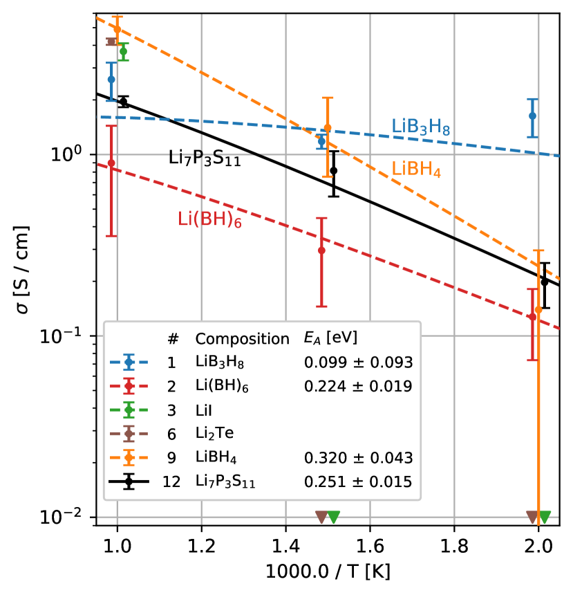
Figure 4: AIMD conductivity values against $1/T$ for the top-$\Xi$ structures. Vertical axis is clipped at minimal conductivity value of $10^{-2}$ S / cm with values below that threshold being indicated as triangles. While the target temperatures in our simulations are exactly 500, 667 and 1000 K, small shifts are added to the horizontal axis values to improve marker visibility. The five LGPS-like structures from the top-$\Xi$ list are omitted from our AIMD studies and therefore not shown in this plot.

III.1 AIMD validation summary

AIMD calculations for the reference Li₇P₃S₁₁ structure result in the activation barrier estimate of $E_{A}=251\pm 15$ meV and room-temperature-extrapolated conductivity of $7.4\pm 2.9$ mS / cm. These are consistent with the range of values measured experimentally, with $E_{A}=295$ meV and $\sigma=8.3$ mS / cm for the most pure phase sample in Ref. [67] and the lowest activation energy of $E_{A}=124$ meV, with $\sigma=3.2$ mS / cm in Ref. [68].

At the top of the list, we find three hydroborate structures, LiB₃H₈ (mp-1211100), Li(BH)₆ (mp-1211296) and LiBH₄ (mp-644223). These belong to the family of lithium hydroborates, of which the best studied is hexagonal LiBH₄ [69, 70, 71]. The latter has been found experimentally to have an ionic conductivity of the order of 1 mS / cm at 383 K. Cubic Li(BH)₆ has been found to have low diffusivity by a combined DFT and ML-IAP study, but a closely connected orthorhombic distortion of the structure was found to have a conductivity of up to 0.1 S / cm at 700 K [72]. In our AIMD calculations, all the three hydroborates show significant ionic mobility in the studied temperature range, although due to the limited statistics we were unable to reliably extrapolate it to room temperature. Since these hydroborates are molecular solids, the anions have rotational degrees of freedom, and these have been shown to be necessary for the high cationic conductivity in Li(BH)₆ [73, 74]. Anionic motion is also apparent on the MSD of the non-Li ions (which we will name the framework) in the AIMD calculations for Li(BH)₆ and LiBH₄.

LiI (mp-570935) also exhibits high mobility at 1000 K, but accompanied by observable diffusivity of the framework ions, which may indicate that 1000 K is close to the melting point. At low temperature, no diffusivity can be observed. Experimentally, wurtzite LiI is metastable and has been observed [75] but is very hygroscopic and hard to work with. Most ionic conductivity studies employing LiI use cubic LiI as a minor fraction of the electrolyte mixture [76].

Finally, Li₂Te (mp-2530) showed high diffusivity only at $T=1000$ K, while no diffusion could be observed at lower temperatures over the affordable simulation times.

Of the five LGPS-like structures from Table 1, Li₁₀Ge(PSe₆)₂ (mp-721239) was simulated in [64], and the reported activation energy and conductivity at room temperature are $190\pm 40$ meV and 24 mS / cm, respectively. The other structure of the same composition, mp-696127, is a slightly less stable concrete realization of the same anion-substituted disordered LGPS-like structure, and the two are expected to be mixed at room temperature. The remaining single Li₁₀Si(PSe₆)₂ and the two concrete realizations of Li₁₀Sn(PSe₆)₂ were not directly studied via AIMD in [64], while individual substitutions of Ge $\rightarrow$ Sn/Si and S $\rightarrow$ Se were all shown to produce superionic materials. Assuming that this also holds for the combined substitutions, we can confirm eight of the ten top-$\Xi$ structures to be superionic.

III.2 ML-driven MD validation summary

Additionally, we perform a larger-scale validation of our results using an ML-IAP as the backbone for the MD. For this study exclusively, we employ the SevenNet model [45]. It has $\sim 4$ times more parameters and is trained on $\sim 10$ times more data than M3GNet, which is used throughout this work, and generally outperforms it on the Matbench Discovery benchmark. The technical details for this SevenNet-driven validation procedure can be found in Appendix A.

We find that 55% of the top-100 $\Xi$-ordered list of structures exhibit room temperature conductivity above 0.1 mS / cm, while that proportion for an unbiased sample is only $\sim 7$% (2 out of 29), as predicted by SevenNet-driven MD. Hence, we observe an approximately 8-fold increase in the number of positive examples through our selection method. At the same time, SevenNet-driven MD predicts room temperature conductivity below 0.005 mS / cm for 39% of the $\Xi$-selected structures. This discrepancy in predictions between our $\Xi$-based selection and SevenNet MD indicates that there likely are mechanisms not captured by the FV descriptors that inhibit high ionic conductivity. It may also be attributed to the limitations of the frozen framework approximation and potential errors in the M3GNet and SevenNet predictions.

III.3 Discussion

Both ML-driven MD and AIMD validation procedures confirm the significant enhancement of the amount of room-temperature superionic materials in the sample selected using the descriptors proposed in this work. Our method achieves even higher-purity samples if we only consider the diffusivity at 1000 K MD simulations: all of the AIMD-tested structures are diffusive at that temperature, and 88% out of top-100 are diffusive in the ML-driven MD validation. This may be due to the fact that most of the positive labels our method was tuned on are found in the Kahle2020 dataset, which consists of primarily $T=1000$ K AIMD diffusion data. In this case, we can expect even higher performance from the proposed method once more high-quality room-temperature conductivity data becomes available.

The highest-$\Xi$ structure we found, LiB₃H₈ (mp-1211100), demonstrates exceptional Li conductivity in our AIMD studies. The SevenNet-driven MD also ranks this material with highest extrapolated room temperature conductivity, which is an order of magnitude higher compared with the same estimate for the reference Li₇P₃S₁₁ material. To the best of our knowledge, this material has not been studied experimentally as a potential SSB electrolyte before, although the similar NaB₃H₈ structure has previously been successfully used in a composite solid electrolyte in a sodium-metal SSB [77, 78]. Ionic conductivity and relaxation times for anionic reorientation have also been studied for various phases of the related KB₃H₈ [79, 80].

The prevalence of the hydroborate structures family at the top of the $\Xi$-ordered list, which are known to be good ionic conductors, demonstrates the remarkable generalization capability of the proposed method. Notably, there are no examples of positively labeled hydroborate electrolytes in either of the datasets that we used for tuning.

Finally, we note that our proposed descriptors are also relatively fast to calculate compared to other methods for predicting superionic materials, including ML-driven MD. Performing the entire PES analysis on the 5997 structures from the Materials Project database took us seven days on a single machine with 48-core Intel Xeon w7-3455 CPU and two 46-GB NVIDIA RTX 6000 Ada Generation GPUs. For comparison, it took us approximately same time to run ML-driven MD for only 100 materials on the same hardware.

III.4 Outlook

The findings presented in this study pave the way for further exploration in the field of ionic conductors for SSBs. Firstly, while our search focused on structures within the Materials Project database, extending this analysis to other databases, such as ICSD [53] and Alexandria [81, 82], is straightforward and may reveal additional promising materials.

Secondly, while the SSE-ranking descriptor $\Xi$ was derived by manually combining the two best-performing descriptors, applying multivariate analysis and ML techniques to the entire set of descriptors could extract even more information from the available data and enhance prediction performance. Moreover, we anticipate that even greater improvements will become evident as more high-quality room-temperature conductivity data becomes available.

Another important direction is the extension of our approach to sodium conductors. We believe that the methodology outlined in our work can be readily applied to identify promising Na-based superionic materials. This could facilitate the advancement of sodium-ion SSBs, which are attracting interest due to their potential for lower costs and abundant raw materials [83].

Finally, the pipeline we have developed is well-suited for generative modeling applications [84, 85]. Both MPE and FV descriptors could be implemented in a differentiable manner, enabling the calculation of gradients with respect to atomic positions and element type embeddings in the underlying machine learning interatomic potential models. These gradients could be utilized in a generative framework to guide the discovery of novel materials with high ionic conductivity.

IV Conclusion

Our study presents an effective method for the rapid screening of solid electrolyte candidates using heuristic descriptors derived from interatomic potentials. By applying our proposed pipeline, supported by a universal machine-learned interatomic potential, we screened 1302 compounds from the Materials Project database, identifying several promising SSE candidates. AIMD simulations of the 10 highest-ranking materials confirm that all are conductive at high temperatures, with 8 out of 10 being superionic at room temperature. Notably, our approach highlights the solid electrolyte LiB₃H₈ (mp-1211100), with an impressive AIMD ionic conductivity estimate of $1.6\pm 0.4$ S / cm at $T=500$ K. To our knowledge, this material has not been studied experimentally in the context of SSBs.

V Data Availability Statement

The code implementing the proposed technique, as well as the predictions calculated for lithium-containing structures from the Materials Project, are available in [63].

VI Acknowledgements

This research project is supported by the Ministry of Education, Singapore, under its Research Centre of Excellence award to the Institute for Functional Intelligent Materials, National University of Singapore (I-FIM, project No. EDUNC-33-18-279-V12). This work used computational resources of the Singapore National Supercomputing Centre (NSCC) of Singapore. For the exploratory phase, this work used computational resources of the Constructor Research Platform provided by Constructor Technologies.

Appendix A Validation with ML-driven MD

We perform an additional validation procedure for our predictions using MD simulations driven by an ML-IAP, which allows to significantly scale up the number of validated structures, as compared to the AIMD studies. While all our PES descriptors are calculated with the M3GNet model [16], we choose the newer SevenNet model [45], which outperforms M3GNet on the Matbench Discovery benchmark [46]. These MD simulations are carried out on 30 random structures satisfying the minimal selection described in Sec. II.2, as well as on the top 100 structures ordered by the $\Xi$ values. Each structure is simulated at two temperature points of 1000 K and 500 K, with step size of 1 fs and total simulation time of 100 ps for each run. Then, the same procedure as for the AIMD studies is used to extract the conductivity values. Figure 5 shows the distributions of the obtained conductivity values. It can be clearly seen from these plots that $\Xi$-based selection significantly enhances the sample with structures with high conductivity at both simulated temperature points and at room temperature, the latter being assessed by extrapolation. In order to demonstrate the level of agreement between AIMD and SevenNet, we plot the two sets of the extracted MSD slope values against each other in Fig. 6. Finally, we present the structures that SevenNet confirmed to be superionic, excluding those previously reported in [29, 26, 11], in Table 2.

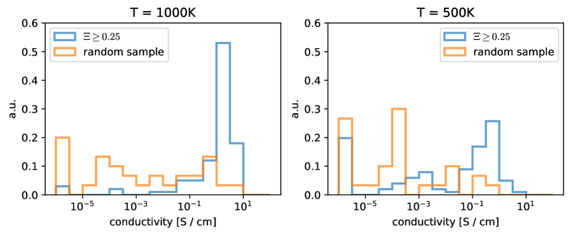
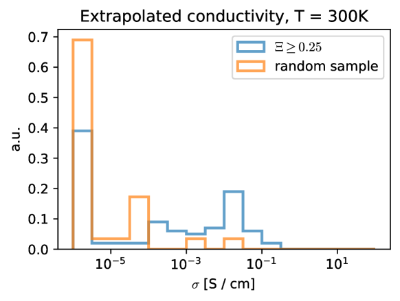
Figure 5: Distributions of conductivities estimated with MD driven by SevenNet. A random sample of size 30 is compared with 100 structures from the top of the $\Xi$-ordered list. In each panel, both histograms are normalized to have the same total weight. The top left (right) panel shows the distributions of values extracted from the $T=1000$ K ($T=500$ K) runs. The bottom panel shows the distributions obtained by extrapolating to the room temperature.

Figure 6: MSD slopes comparison between AIMD and SevenNet-driven MD. All values are clipped from below at $10^{-3}$ $\AA^{2}$ / ps. The dashed black line denotes the set of points with $x=y$.

MP identifier	Composition	$\Xi$
mp-1211100	LiB3H8	0.992
mp-1211296	Li(BH)6	0.99
mp-985583	Li3PS4	0.958
mp-1001069	Li48P16S61	0.956
mp-1097034	Li20Si3P3S23Cl	0.951
mp-1040451	Li20Si3P3S23Cl	0.949
mp-1185263	LiPaO3	0.942
mp-1097036	Li3PS4	0.931
mp-1222398	LiGa(GeSe3)2	0.896
mp-755463	Li3SbS3	0.887
mp-753720	Li3BiS3	0.858
mp-1222392	LiUI6	0.82
mp-34038	Li6NCl3	0.814
mp-680395	Li3As7	0.783
mp-775806	Li3SbS3	0.763
mp-28336	Li3P7	0.721
mp-1222582	Li4GeS4	0.717
mp-753429	Li4Bi2S7	0.716
mp-985582	Li6PS5I	0.703
mp-1177520	Li3SbS3	0.658
mp-1211362	Li(BH)6	0.647
mp-1211446	Li7PSe6	0.606
mp-1222482	Li6AsS5I	0.539
mp-1211324	Li7PS6	0.538
mp-1195718	Li4SnS4	0.525
mp-950995	Li6PS5I	0.521
mp-1211176	Li6AsS5I	0.483

Table 2: Top-$\Xi$ candidates confirmed with SevenNet MD that were not predicted in [29, 26, 11]. Reported are the 27 structures (25 after excluding the two containing rare and radioactive elements) from the top-100 highest $\Xi$ list that have extrapolated room temperature conductivity above 1 mS / cm, as predicted with SevenNet MD. Structures already reported in [29, 26, 11] were excluded from this list.

Appendix B Comparison of FV descriptors with AIMD and experimental labels

Figures 7 and 8 demonstrate scatter plots with relationships between the labels from the Kahle2020 and Laskowski2023 datasets, respectively, and the connected and disconnected versions of the FV descriptor at the threshold of 0.5 eV.

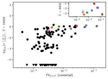
(a)

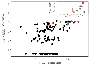
(b)

Figure 7: Distributions of conductivity labels against FV descriptors for the simulated dataset. Shown are such distributions for the connected (left) and disconnected (right) versions of the FV descriptors at the threshold of 0.5 eV. The conductivity labels are taken from the 1000 K temperature point in the main plots, while the inset plots show such distributions for the room-temperature-extrapolated conductivity values. As the extrapolated temperature entries are a small subset of the whole dataset, they use per-structure colors in order to relate same structures between the two temperature points. Since the method for extracting the diffusivity constants used in [10] allows for small negative values, such values are clipped at $\sigma=10^{-7}$ S / cm to be kept in the log-scale and shown as triangles in the plots.

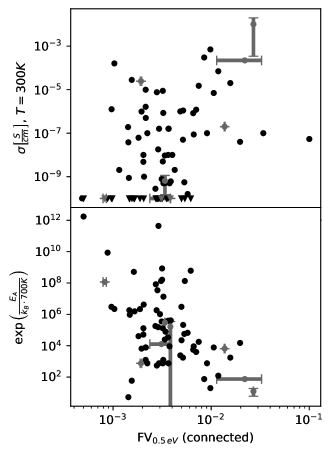
(a)

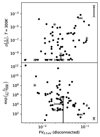
(b)

Figure 8: Distributions of conductivity and activation energy labels against FV descriptors for the experimental dataset. Shown are such distributions for the connected (left) and disconnected (right) versions of the FV descriptors at the threshold of 0.5 eV. The top panels show the distributions for the conductivities at room temperature. Extremely low conductivity values are clipped at $\sigma=10^{-10}$ S / cm and are shown as triangles in the plot. The bottom panels demonstrate the activation energies provided in the Laskowski2023 dataset converted to a multiplicative factor relating diffusion constants between $T=1000$ K and $T=300$ K via the Arrhenius law. Horizontal error bars are provided for the structures taken from ICSD, where partial occupancy sites are present and a number of concrete structures are sampled. Vertical error bars are shown for the cases where multiple measurements are provided for a single structure.

Appendix C Alternative ranking models

The ranking descriptor $\Xi$ from Eq. 4 was originally constructed through a visual examination of Figs. 3, 7 and 8. In this section, we describe our work to develop an improved ranking model, using a multivariate analysis of all the introduced descriptors (MPE and FV), referred to collectively as the PES descriptors. Additionally, we incorporate the descriptors from the matminer library [40], following [26], to evaluate the relative performance of the two descriptor sets, as well as their combined utility.

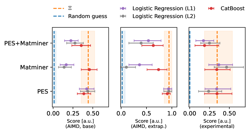
Figure 9: Evaluation scores for models trained on the Kahle2020 dataset using various sets of descriptors. The scoring procedure is the same as for the results presented in Fig. 3.

To make this comparison, we train classification models on the Kahle2020 dataset with $T=1000$ K labels, as defined in Sec. II.2, and evaluate them using the procedure outlined in that section. The Leave-One-Out cross-validation technique was employed for model training, where each individual sample is sequentially left out for testing while the remaining samples are used for training. The following three multivariate analysis models were trained: two versions of logistic regression, with L1 and L2 regularization terms, respectively, as implemented in [86], as well as the CatBoost [87] implementation of gradient boosting on decision trees. Each model was separately trained on three feature representations: based on PES descriptors alone, based on matminer descriptors alone, as well as on the combination of both. Resulting scores are shown in Fig. 9.

From Fig. 9, it appears that none of the models outperform the $\Xi$ descriptor. Models trained exclusively on the matminer descriptors show reasonable scores on the Laskowski2023 experimental dataset, but they sacrifice predictive power on the AIMD data.

Appendix D Alternative MSD fitting window parameters

Along with the MSD fitting procedure described in the main text, we consider three alternative options. The first option is to fit the entire MSD trajectory, which doesn’t allow to properly estimate the uncertainty of the result but is most sensitive to slowest diffusion processes. The two remaining options are alternative windowed configurations with fitted MSD interval starting from 0 ps and 5 ps, respectively, as opposed to 1 ps chosen in the main procedure. The comparison of the results obtained with the main and the three alternative procedures is shown in Fig. 10. We can clearly see that all four approaches agree in high diffusion regime. In the slow diffusion region, fitting each window from 0 ps overestimates the slopes of MSD due to periodic atomic movement and therefore is inapplicable. Windowed fits with later starting point of 5 ps produce results that are consistent with the 1 ps starting point fits.

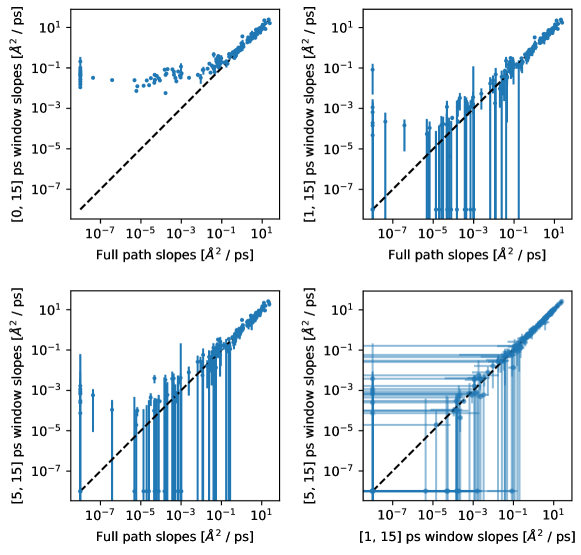
Figure 10: MSD slope values extracted with different fitting window parameters. The results of single fits for the entire simulated trajectory (horizontal axes) are compared with various windowed fit configurations (vertical axes) in top left, top right and bottom left panels, while bottom right panel compares two windowed fit configurations against each other. All windowed fits are performed for 15 ps windows. The starting point of the windowed fits is 0 ps in the top left panel, 1 ps in the top right panel and 5 ps in the bottom left panel. Bottom right panel compares 1 ps and 5 ps fit starting points. The values are extracted from all the SevenNet MD and AIMD runs performed. All values are clipped from below at $10^{-8}$ $\AA^{2}$ / ps. The dashed black line denotes the set of points with $x=y$.

References

- Kim et al. [2015] J. G. Kim, B. Son, S. Mukherjee, N. Schuppert, A. Bates, O. Kwon, M. J. Choi, H. Y. Chung, and S. Park, A review of lithium and non-lithium based solid state batteries, J. Power Sources 282, 299 (2015).
- Li et al. [2021] C. Li, Z. Wang, Z. He, Y. Li, J. Mao, K. Dai, C. Yan, and J. Zheng, An advance review of solid-state battery: challenges, progress and prospects, SM&T 29, e00297 (2021).
- Janek and Zeier [2023] J. Janek and W. G. Zeier, Challenges in speeding up solid-state battery development, Nat. Energy. 8, 230 (2023).
- Dudney et al. [2015] N. J. Dudney, W. C. West, and J. Nanda, Handbook of solid state batteries, 2nd ed., Vol. 6 (World Scientific, Singapore, 2015).
- Zhao et al. [2020] Q. Zhao, S. Stalin, C.-Z. Zhao, and L. A. Archer, Designing solid-state electrolytes for safe, energy-dense batteries, Nature Reviews Materials 5, 229 (2020).
- Chen et al. [2021] C. Chen, M. Jiang, T. Zhou, L. Raijmakers, E. Vezhlev, B. Wu, T. U. Schülli, D. L. Danilov, Y. Wei, R.-A. Eichel, et al., Interface aspects in all-solid-state Li-based batteries reviewed, Advanced energy materials 11, 2003939 (2021).
- Ohta et al. [2006] N. Ohta, K. Takada, L. Zhang, R. Ma, M. Osada, and T. Sasaki, Enhancement of the high-rate capability of solid-state lithium batteries by nanoscale interfacial modification, Advanced Materials 18, 2226 (2006).
- Rodin et al. [2022] A. Rodin, K. Noori, A. Carvalho, and A. H. Castro Neto, Microscopic theory of ionic motion in solids, Phys. Rev. B 105, 224310 (2022).
- Carvalho et al. [2022] A. Carvalho, S. Negi, and A. H. C. Neto, Direct calculation of the ionic mobility in superionic conductors, Scientific Reports 12, 19930 (2022).
- Kahle et al. [2020] L. Kahle, A. Marcolongo, and N. Marzari, High-throughput computational screening for solid-state li-ion conductors, Energy Environ. Sci. 13, 928 (2020).
- Muy et al. [2019] S. Muy, J. Voss, R. Schlem, R. Koerver, S. J. Sedlmaier, F. Maglia, P. Lamp, W. G. Zeier, and Y. Shao-Horn, High-throughput screening of solid-state Li-ion conductors using lattice-dynamics descriptors, iScience 16, 270 (2019).
- Wang et al. [2015] Y. Wang, W. D. Richards, S. P. Ong, L. J. Miara, J. C. Kim, Y. Mo, and G. Ceder, Design principles for solid-state lithium superionic conductors, Nature materials 14, 1026 (2015).
- Schütt et al. [2017] K. Schütt, P.-J. Kindermans, H. E. Sauceda Felix, S. Chmiela, A. Tkatchenko, and K.-R. Müller, Schnet: A continuous-filter convolutional neural network for modeling quantum interactions, Advances in neural information processing systems 30 (2017).
- Xie and Grossman [2018] T. Xie and J. C. Grossman, Crystal graph convolutional neural networks for an accurate and interpretable prediction of material properties, Physical review letters 120, 145301 (2018).
- Chen et al. [2019] C. Chen, W. Ye, Y. Zuo, C. Zheng, and S. P. Ong, Graph networks as a universal machine learning framework for molecules and crystals, Chemistry of Materials 31, 3564 (2019).
- Chen and Ong [2022] C. Chen and S. P. Ong, A universal graph deep learning interatomic potential for the periodic table, Nature Computational Science 2, 718 (2022).
- Deng et al. [2023] B. Deng, P. Zhong, K. Jun, J. Riebesell, K. Han, C. J. Bartel, and G. Ceder, CHGNet as a pretrained universal neural network potential for charge-informed atomistic modelling, Nature Machine Intelligence 5, 1031 (2023).
- Batatia et al. [2022a] I. Batatia, S. Batzner, D. P. Kovács, A. Musaelian, G. N. C. Simm, R. Drautz, C. Ortner, B. Kozinsky, and G. Csányi, The design space of e(3)-equivariant atom-centered interatomic potentials, arXiv:2205.06643 (2022a).
- Batatia et al. [2022b] I. Batatia, D. P. Kovacs, G. N. C. Simm, C. Ortner, and G. Csanyi, MACE: Higher order equivariant message passing neural networks for fast and accurate force fields, in Advances in Neural Information Processing Systems, edited by A. H. Oh, A. Agarwal, D. Belgrave, and K. Cho (2022).
- Batatia et al. [2023] I. Batatia, P. Benner, Y. Chiang, A. M. Elena, D. P. Kovács, J. Riebesell, X. R. Advincula, M. Asta, W. J. Baldwin, N. Bernstein, et al., A foundation model for atomistic materials chemistry, arXiv:2401.00096 (2023).
- Merchant et al. [2023] A. Merchant, S. Batzner, S. S. Schoenholz, M. Aykol, G. Cheon, and E. D. Cubuk, Scaling deep learning for materials discovery, Nature 624, 80 (2023).
- Zeni et al. [2024] C. Zeni, R. Pinsler, D. Zügner, A. Fowler, M. Horton, X. Fu, S. Shysheya, J. Crabbé, L. Sun, J. Smith, B. Nguyen, H. Schulz, S. Lewis, C.-W. Huang, Z. Lu, Y. Zhou, H. Yang, H. Hao, J. Li, R. Tomioka, and T. Xie, Mattergen: a generative model for inorganic materials design, arXiv:2312.03687 (2024).
- Liu et al. [2021] H. Liu, S. Ma, J. Wu, Y. Wang, and X. Wang, Recent advances in screening lithium solid-state electrolytes through machine learning, Frontiers in Energy Research 9, 639741 (2021).
- Hu et al. [2022] Q. Hu, K. Chen, F. Liu, M. Zhao, F. Liang, and D. Xue, Smart materials prediction: Applying machine learning to lithium solid-state electrolyte, Materials 15, 1157 (2022).
- Jain et al. [2013] A. Jain, S. P. Ong, G. Hautier, W. Chen, W. D. Richards, S. Dacek, S. Cholia, D. Gunter, D. Skinner, G. Ceder, and K. A. Persson, Commentary: The materials project: A materials genome approach to accelerating materials innovation, APL materials 1, 011002 (2013).
- Laskowski et al. [2023] F. A. Laskowski, D. B. McHaffie, and K. A. See, Identification of potential solid-state li-ion conductors with semi-supervised learning, Energy & Environmental Science 16, 1264 (2023).
- Sendek et al. [2020] A. D. Sendek, G. Cheon, M. Pasta, and E. J. Reed, Quantifying the search for solid li-ion electrolyte materials by anion: a data-driven perspective, The Journal of Physical Chemistry C 124, 8067 (2020).
- Sendek et al. [2017] A. D. Sendek, Q. Yang, E. D. Cubuk, K.-A. N. Duerloo, Y. Cui, and E. J. Reed, Holistic computational structure screening of more than 12000 candidates for solid lithium-ion conductor materials, Energy & Environmental Science 10, 306 (2017).
- Sendek et al. [2019] A. D. Sendek, E. D. Cubuk, E. R. Antoniuk, G. Cheon, Y. Cui, and E. J. Reed, Machine learning-assisted discovery of solid Li-ion conducting materials, Chemistry of Materials 31, 342 (2019).
- Choi et al. [2021] E. Choi, J. Jo, W. Kim, and K. Min, Searching for mechanically superior solid-state electrolytes in li-ion batteries via data-driven approaches, ACS applied materials & interfaces 13, 42590 (2021).
- Fujimura et al. [2013] K. Fujimura, A. Seko, Y. Koyama, A. Kuwabara, I. Kishida, K. Shitara, C. A. Fisher, H. Moriwake, and I. Tanaka, Accelerated materials design of lithium superionic conductors based on first-principles calculations and machine learning algorithms, Advanced Energy Materials 3, 980 (2013).
- Cubuk et al. [2019] E. D. Cubuk, A. D. Sendek, and E. J. Reed, Screening billions of candidates for solid lithium-ion conductors: A transfer learning approach for small data, The Journal of chemical physics 150 (2019).
- Zhang et al. [2019] Y. Zhang, X. He, Z. Chen, Q. Bai, A. M. Nolan, C. A. Roberts, D. Banerjee, T. Matsunaga, Y. Mo, and C. Ling, Unsupervised discovery of solid-state lithium ion conductors, Nature communications 10, 5260 (2019).
- Ahmad et al. [2018] Z. Ahmad, T. Xie, C. Maheshwari, J. C. Grossman, and V. Viswanathan, Machine learning enabled computational screening of inorganic solid electrolytes for suppression of dendrite formation in lithium metal anodes, ACS central science 4, 996 (2018).
- Wang et al. [2023] Z. Wang, Y. Han, J. Cai, A. Chen, and J. Li, An end-to-end artificial intelligence platform enables real-time assessment of superionic conductors, SmartMat 4, e1183 (2023).
- Guo et al. [2024] X. Guo, Z. Wang, J.-H. Yang, and X.-G. Gong, Machine-learning assisted high-throughput discovery of solid-state electrolytes for li-ion batteries, Journal of Materials Chemistry A 12, 10124 (2024).
- Nishitani et al. [2018] Y. Nishitani, S. Adams, K. Ichikawa, and T. Tsujita, Evaluation of magnesium ion migration in inorganic oxides by the bond valence site energy method, Solid State Ionics 315, 111 (2018).
- Jang et al. [2022] S.-H. Jang, Y. Tateyama, and R. Jalem, High-Throughput Data-Driven Prediction of Stable High-Performance Na-Ion Sulfide Solid Electrolytes, Advanced Functional Materials 32, 2206036 (2022).
- He et al. [2020] B. He, S. Chi, A. Ye, P. Mi, L. Zhang, B. Pu, Z. Zou, Y. Ran, Q. Zhao, D. Wang, et al., High-throughput screening platform for solid electrolytes combining hierarchical ion-transport prediction algorithms, Scientific Data 7, 151 (2020).
- Ward et al. [2018] L. Ward, A. Dunn, A. Faghaninia, N. E. Zimmermann, S. Bajaj, Q. Wang, J. Montoya, J. Chen, K. Bystrom, M. Dylla, K. Chard, M. Asta, K. A. Persson, G. J. Snyder, I. Foster, and A. Jain, Matminer: An open source toolkit for materials data mining, Computational Materials Science 152, 60 (2018).
- Behler and Parrinello [2007] J. Behler and M. Parrinello, Generalized neural-network representation of high-dimensional potential-energy surfaces, Physical review letters 98, 146401 (2007).
- Bartók et al. [2010] A. P. Bartók, M. C. Payne, R. Kondor, and G. Csányi, Gaussian approximation potentials: The accuracy of quantum mechanics, without the electrons, Physical review letters 104, 136403 (2010).
- Thompson et al. [2015] A. P. Thompson, L. P. Swiler, C. R. Trott, S. M. Foiles, and G. J. Tucker, Spectral neighbor analysis method for automated generation of quantum-accurate interatomic potentials, Journal of Computational Physics 285, 316 (2015).
- Batzner et al. [2022] S. Batzner, A. Musaelian, L. Sun, M. Geiger, J. P. Mailoa, M. Kornbluth, N. Molinari, T. E. Smidt, and B. Kozinsky, E (3)-equivariant graph neural networks for data-efficient and accurate interatomic potentials, Nature communications 13, 2453 (2022).
- Park et al. [2024] Y. Park, J. Kim, S. Hwang, and S. Han, Scalable parallel algorithm for graph neural network interatomic potentials in molecular dynamics simulations, Journal of Chemical Theory and Computation 20, 4857 (2024), pMID: 38813770.
- Riebesell et al. [2023] J. Riebesell, R. E. A. Goodall, P. Benner, Y. Chiang, B. Deng, A. A. Lee, A. Jain, and K. A. Persson, Matbench Discovery – A framework to evaluate machine learning crystal stability predictions, arXiv:2308.14920 (2023).
- Jónsson et al. [1998] H. Jónsson, G. Mills, and K. W. Jacobsen, Nudged elastic band method for finding minimum energy paths of transitions, in Classical and quantum dynamics in condensed phase simulations (World Scientific, 1998) pp. 385–404.
- Zeng et al. [2023] J. Zeng, D. Zhang, D. Lu, P. Mo, Z. Li, Y. Chen, M. Rynik, L. Huang, Z. Li, S. Shi, Y. Wang, H. Ye, P. Tuo, J. Yang, Y. Ding, Y. Li, D. Tisi, Q. Zeng, H. Bao, Y. Xia, J. Huang, K. Muraoka, Y. Wang, J. Chang, F. Yuan, S. L. Bore, C. Cai, Y. Lin, B. Wang, J. Xu, J.-X. Zhu, C. Luo, Y. Zhang, R. E. A. Goodall, W. Liang, A. K. Singh, S. Yao, J. Zhang, R. Wentzcovitch, J. Han, J. Liu, W. Jia, D. M. York, W. E, R. Car, L. Zhang, and H. Wang, DeePMD-kit v2: A software package for deep potential models, J. Chem. Phys. 159, 054801 (2023).
- Qi et al. [2024] J. Qi, T. W. Ko, B. C. Wood, T. A. Pham, and S. P. Ong, Robust training of machine learning interatomic potentials with dimensionality reduction and stratified sampling, npj Computational Materials 10, 43 (2024).
- Morimoto et al. [2019] T. Morimoto, M. Nagai, Y. Minowa, M. Ashida, Y. Yokotani, Y. Okuyama, and Y. Kani, Microscopic ion migration in solid electrolytes revealed by terahertz time-domain spectroscopy, Nature communications 10, 2662 (2019).
- van der Maas et al. [2023] E. van der Maas, T. Famprikis, S. Pieters, J. P. Dijkstra, Z. Li, S. R. Parnell, R. I. Smith, E. R. van Eck, S. Ganapathy, and M. Wagemaker, Re-investigating the structure–property relationship of the solid electrolytes Li3-x In1-x Zrx Cl6 and the impact of In–Zr (iv) substitution, Journal of Materials Chemistry A 11, 4559 (2023).
- Momma and Izumi [2011] K. Momma and F. Izumi, VESTA3 for three-dimensional visualization of crystal, volumetric and morphology data, Journal of Applied Crystallography 44, 1272 (2011).
- Zagorac et al. [2019] D. Zagorac, H. Müller, S. Ruehl, J. Zagorac, and S. Rehme, Recent developments in the Inorganic Crystal Structure Database: theoretical crystal structure data and related features, Journal of applied crystallography 52, 918 (2019).
- Soler et al. [2002] J. M. Soler, E. Artacho, J. D. Gale, A. García, J. Junquera, P. Ordejón, and D. Sánchez-Portal, The SIESTA method for ab initio order-N materials simulation, J. Phys.: Condens. Matter 14, 2745 (2002).
- Perdew et al. [1996] J. P. Perdew, K. Burke, and M. Ernzerhof, Generalized gradient approximation made simple, Phys. Rev. Lett. 77, 3865 (1996).
- Lee et al. [2010] K. Lee, É. D. Murray, L. Kong, B. I. Lundqvist, and D. C. Langreth, Higher-accuracy van der Waals density functional, Physical Review B 82, 081101 (2010).
- Dion et al. [2004] M. Dion, H. Rydberg, E. Schröder, D. C. Langreth, and B. I. Lundqvist, Van der Waals Density Functional for General Geometries, Phys. Rev. Lett. 92, 246401 (2004).
- Troullier and Martins [1991] N. Troullier and J. L. Martins, Efficient pseudopotentials for plane-wave calculations, Physical Review B 43, 1993 (1991).
- Sánchez-Portal et al. [1997] D. Sánchez-Portal, P. Ordejon, E. Artacho, and J. M. Soler, Density-functional method for very large systems with lcao basis sets, International journal of quantum chemistry 65, 453 (1997).
- Sánchez-Portal et al. [2001] D. Sánchez-Portal, J. Junquera, Ó. Paz, and E. Artacho, Numerical atomic orbitals for linear-scaling calculations, Phys. Rev. B 64, 235111 (2001).
- Monkhorst and Pack [1976] H. J. Monkhorst and J. D. Pack, Special points for brillouin-zone integrations, Physical Review B 13, 5188 (1976).
- Nosé [1984] S. Nosé, A unified formulation of the constant temperature molecular dynamics methods, J. Chem. Phys. 81, 511 (1984).
- ML4 [2024] (2024), https://constructor.app/platform/public/project/pes_fingerprint.
- Ong et al. [2013] S. P. Ong, Y. Mo, W. D. Richards, L. Miara, H. S. Lee, and G. Ceder, Phase stability, electrochemical stability and ionic conductivity of the Li10±1MP2X12 (M = Ge, Si, Sn, Al or P, and X = O, S or Se) family of superionic conductors, Energy Environ. Sci. 6, 148 (2013).
- Yamane et al. [2007] H. Yamane, M. Shibata, Y. Shimane, T. Junke, Y. Seino, S. Adams, K. Minami, A. Hayashi, and M. Tatsumisago, Crystal structure of a superionic conductor, Li7P3S11, Solid State Ionics 178, 1163 (2007).
- Kamaya et al. [2011] N. Kamaya, K. Homma, Y. Yamakawa, M. Hirayama, R. Kanno, M. Yonemura, T. Kamiyama, Y. Kato, S. Hama, K. Kawamoto, and A. Mitsui, A lithium superionic conductor, Nature materials 10, 682 (2011).
- Busche et al. [2016] M. R. Busche, D. A. Weber, Y. Schneider, C. Dietrich, S. Wenzel, T. Leichtweiss, D. Schröder, W. Zhang, H. Weigand, D. Walter, S. J. Sedlmaier, D. Houtarde, L. F. Nazar, and J. Janek, In situ monitoring of fast Li-ion conductor Li7P3S11 crystallization inside a hot-press setup, Chemistry of Materials 28, 6152 (2016).
- Mizuno et al. [2006] F. Mizuno, A. Hayashi, K. Tadanaga, and M. Tatsumisago, High lithium ion conducting glass-ceramics in the system Li2S–P2S5, Solid State Ionics 177, 2721 (2006).
- Matsuo et al. [2007] M. Matsuo, Y. Nakamori, S.-i. Orimo, H. Maekawa, and H. Takamura, Lithium superionic conduction in lithium borohydride accompanied by structural transition, Applied Physics Letters 91, 224103 (2007).
- Duchêne et al. [2020] L. Duchêne, A. Remhof, H. Hagemann, and C. Battaglia, Status and prospects of hydroborate electrolytes for all-solid-state batteries, Energy Storage Materials 25, 782 (2020).
- Liu et al. [2023] H. Liu, X. Zhou, M. Ye, and J. Shen, Ion migration mechanism study of hydroborate/carborate electrolytes for all-solid-state batteries, Electrochemical Energy Reviews 6, 31 (2023).
- Maltsev et al. [2023] A. P. Maltsev, I. V. Chepkasov, and A. R. Oganov, Order–disorder phase transition and ionic conductivity in a Li2B12H12 solid electrolyte, ACS Applied Materials & Interfaces 15, 42511 (2023).
- Lu and Ciucci [2017] Z. Lu and F. Ciucci, Metal borohydrides as electrolytes for solid-state li, na, mg, and ca batteries: a first-principles study, Chemistry of Materials 29, 9308 (2017).
- Kweon et al. [2017] K. E. Kweon, J. B. Varley, P. Shea, N. Adelstein, P. Mehta, T. W. Heo, T. J. Udovic, V. Stavila, and B. C. Wood, Structural, chemical, and dynamical frustration: origins of superionic conductivity in closo-borate solid electrolytes, Chemistry of Materials 29, 9142 (2017).
- Wassermann et al. [1988] B. Wassermann, W. Hönle, and T. Martin, Hexagonal LiI, Solid state communications 65, 561 (1988).
- Poulsen [1981] F. W. Poulsen, Ionic conductivity of solid lithium iodide and its monohydrate, Solid State Ionics 2, 53 (1981).
- Qiu et al. [2024] P. Qiu, X. Chen, W. Zhang, G. Zhang, Y. Zhang, Z. Lu, Y. Wu, and X. Chen, A High-Rate and Long-Life Sodium Metal Battery Based on a NaB3H8 xNH3@NaB3H8 Composite Solid-State Electrolyte, Angewandte Chemie International Edition 63, e202401480 (2024).
- Chen et al. [2024] X.-W. Chen, J.-X. Kang, Z.-H. Fan, N. Zhang, W.-Y. Zhang, G.-G. Zhang, A.-Q. Zhu, Z.-W. Lu, P. Qiu, Y. Wu, and X. Chen, Sodium octahydridotriborate as a solid electrolyte with excellent stability against sodium-metal anode, Small 20, 2401439 (2024).
- Grinderslev et al. [2019] J. B. Grinderslev, K. T. Møller, Y. Yan, X.-M. Chen, Y. Li, H.-W. Li, W. Zhou, J. Skibsted, X. Chen, and T. R. Jensen, Potassium octahydridotriborate: diverse polymorphism in a potential hydrogen storage material and potassium ion conductor, Dalton Trans. 48, 8872 (2019).
- Andersson et al. [2021] M. S. Andersson, J. B. Grinderslev, X.-M. Chen, X. Chen, U. Häussermann, W. Zhou, T. R. Jensen, M. Karlsson, and T. J. Udovic, Interplay between the Reorientational Dynamics of the B3H8- Anion and the Structure in KB3H8, The Journal of Physical Chemistry C 125, 3716 (2021).
- [81] Alexandria databases, https://alexandria.icams.rub.de/, accessed: 2024-10-04.
- Schmidt et al. [2023] J. Schmidt, N. Hoffmann, H.-C. Wang, P. Borlido, P. J. M. A. Carriço, T. F. T. Cerqueira, S. Botti, and M. A. L. Marques, Machine-learning-assisted determination of the global zero-temperature phase diagram of materials, Advanced Materials 35, 2210788 (2023).
- Yang et al. [2021] H.-L. Yang, B.-W. Zhang, K. Konstantinov, Y.-X. Wang, H.-K. Liu, and S.-X. Dou, Progress and challenges for all-solid-state sodium batteries, Advanced Energy and Sustainability Research 2, 2000057 (2021).
- Al-Maeeni et al. [2024] A. Al-Maeeni, M. Lazarev, N. Kazeev, K. S. Novoselov, and A. Ustyuzhanin, Review on automated 2D material design, 2D Materials 11, 032002 (2024).
- Anonymous [2024] Anonymous, Wyckoff transformer: Generation of symmetric crystals, in Submitted to The Thirteenth International Conference on Learning Representations (2024) under review.
- Pedregosa et al. [2011] F. Pedregosa, G. Varoquaux, A. Gramfort, V. Michel, B. Thirion, O. Grisel, M. Blondel, P. Prettenhofer, R. Weiss, V. Dubourg, J. Vanderplas, A. Passos, D. Cournapeau, M. Brucher, M. Perrot, and E. Duchesnay, Scikit-learn: Machine learning in Python, Journal of Machine Learning Research 12, 2825 (2011).
- Dorogush et al. [2018] A. V. Dorogush, V. Ershov, and A. Gulin, Catboost: gradient boosting with categorical features support, arXiv:1810.11363 (2018).