A System Parametrization for Direct Data-Driven Analysis and Control with Error-in-Variables

Abstract

In this paper, we present a new parametrization to perform direct data-driven analysis and controller synthesis for the error-in-variables case. To achieve this, we employ the Sherman-Morrison-Woodbury formula to transform the problem into a linear fractional transformation (LFT) with unknown measurement errors and disturbances as uncertainties. For bounded uncertainties, we apply robust control techniques to derive a guaranteed upper bound on the $\mathcal{H}_{2}$-norm of the unknown true system. To this end, a single semidefinite program (SDP) needs to be solved, with complexity that is independent of the amount of data. Furthermore, we exploit the signal-to-noise ratio to provide a data-dependent condition, that characterizes whether the proposed parametrization can be employed. The modular formulation allows to extend this framework to controller synthesis with different performance criteria, input-output settings, and various system properties. Finally, we validate the proposed approach through a numerical example.

I INTRODUCTION

In recent years, interest in system analysis and controller design based on collected data has been continuously increasing [1, 2, 3]. Indirect data-driven control first identifies a model to employ model-based techniques for controller design and analysis as a second step. In practice, only a finite number of possibly noisy data points are available, making identifying the true system challenging in many cases, even for the linear case [4]. This mismatch between the true and identified model may lead to instabilities or deteriorated performance guarantees when applying the controller to the true system.

A possible remedy is offered by direct data-driven control, where end-to-end guarantees can be provided even for a finite number of noisy data samples [5]. Here, available results are often restricted to bounded noise, which includes, e.g., energy bounds and individual noise bounds for each time instance. Many results in the literature build on the data-informativity framework [6, 7], which provides stability and performance guarantees for the true system by verifying a desired property for all systems consistent with the data. Another direct data-driven approach relies on parameterizing the set of consistent system matrices in terms of a right inverse of the stacked data matrices [8, 9].

Most existing works consider only the case of additive process noise [10, 11]. Although additive process noise often appears in linear dynamical systems, it is also possible to approximate nonlinear systems via basis functions and treat the resulting approximation error as an additive disturbance [3]. By deriving a bound on the approximation error, it is possible to provide guarantees for unknown nonlinear systems.

When collecting data, the occurring measurement noise introduces yet another error source leading to the error-in-variables problem. Without explicitly addressing the measurement noise, the derived analysis often results in biases. For example, in the linear least squares problem, not considering error-in-variables results in systematically smaller parameters [12].

In system identification, the bias can be eliminated based on set-membership estimation, where the set of consistent systems is identified [13]. Similarly, [14] designs a stabilizing controller using such an identified set. To achieve this, the authors reformulate the problem as a sum-of-squares problem, which can be solved iteratively using SDPs. To design guaranteed stabilizing controllers for sufficiently small measurement noise, an alternative is to introduce a regularization term to a predictive controller based on Hankel matrices [15]. This leads to a trade-off between a simple parametrization and reliance on data. Moreover, [8] treats error-in-variables as additive process noise, which requires additional knowledge of the singular values of the true system. However, this knowledge may not always be available. Recent results extend the data-informativity setting to the case with error-in-variables under the assumption that the process noise and the measurement error satisfy a particular quadratic matrix inequality [16] .

In this work, we derive an explicit and exact parametrization of all systems consistent with the data by interpreting the data-driven control problem as linear regression. The main contribution of this paper is to generalize the results of [8, 11] to the errors-in-variables problem. Moreover the proposed parameterization allows for a more flexible description of the noise affecting the data than the data-informativity framework, while still requiring the solution of only a single SDP. Furthermore, we exemplify the use of the derived parametrization to compute an upper bound on the $\mathcal{H}_{2}$-norm of the true unknown system. Finally, by formulating the parameterization in terms of an LFT, many already existing methods from robust control can be applied to extend this setup for different performance criteria, noise descriptions and controller design adding flexibility.

II PRELIMINARIES

We denote the $n\times n$ identity matrix and the $p\times q$ zero matrix as $I_{n}$ and $0_{p\times q}$, respectively, where we omit the indices if the dimensions are clear from the context. For the sake of space limitations, we use $\star$ if the corresponding matrix block can be inferred from symmetry. Moreover, we use $P\succ 0$ and $P\succeq 0$ if the symmetric matrix $P$ is positive definite or positive semidefinite. Negative (semi-)definiteness is defined by $P\prec 0$ and $P\preceq 0$, respectively. We use $\mathrm{diag}(V_{1},V_{2})$ to describe a block diagonal matrix with $V_{1}$ and $V_{2}$ on its diagonal. Moreover, we use $\sigma_{\mathrm{min}}(A)$ and $\sigma_{\mathrm{max}}(A)$ to denote the minimal and maximal singular value of $A$. For measurements $\{x_{k}\}_{k=0}^{N}$, we define the following matrices

$$X=\begin{bmatrix}x_{0}&x_{1}&\ldots&x_{N-1}\end{bmatrix},\text{ }X_{+}=\begin{bmatrix}x_{1}&x_{2}&\ldots&x_{N}\end{bmatrix}.$$

In this paper, we consider matrices with unknown elements. In particular, we look at LFTs.

Definition 1

The linear fractional transformation

$$\begin{bmatrix}y\\ z\end{bmatrix} =\left[\begin{array}[]{cc}A&B\\ C&D\\ \end{array}\right]\begin{bmatrix}x\\ w\end{bmatrix}, w =\delta z$$ (3)

is well-posed if $(I-D\delta)$ is non-singular.

In this work, we treat $\delta$ as unknown. Furthermore, a well-posed LFT can equivalently be written as

$$y=\left(A+B\delta\left(I-D\delta\right)^{-1}C\right)x.$$ (4)

The next lemma is key in deriving an LFT formulation in Section III.

Lemma 1

Let $I+UV$ be invertible. Then the following equality holds

$$(I+UV)^{-1}=I-U(I+VU)^{-1}V.$$ (5)

This is a special case of the well-known Sherman–Morrison–Woodbury formula, which is used to efficiently compute a matrix inverse with low-rank updates [17, 18].

In Section IV, we treat a linear-time-invariant (LTI)-system as LFT, for which we define the following norm.

Definition 2

The $\mathcal{H}_{2}$-norm of an asymptotically stable, discrete-time transfer function $P$ is

$$||P(e^{\mathrm{j}\omega}))||_{2}=\sqrt{\frac{1}{2\pi}\int\limits_{-\pi}^{\pi}\mathrm{trace}(P(e^{\mathrm{j}\omega})^{*}P(e^{\mathrm{j}\omega}))\,\mathrm{d}\omega}$$ (6)

with ^∗ denoting the conjugate transpose.

The squared $\mathcal{H}_{2}$-norm coincides with the total output-energy of the impulse response [19].

III DATA-DRIVEN SYSTEM PARAMETRIZATION

In this work, we consider a linear regression model of the form

$$y=\Theta_{\mathrm{tr}}x,$$ (7)

with regressand $y\in\mathbb{R}^{p}$, regressor $x\in\mathbb{R}^{n}$ and unknown true parameter matrix $\Theta_{\mathrm{tr}}\in\mathbb{R}^{p\times n}$. Our goal is to find an LFT parametrization of the true parameter matrix $\Theta_{\mathrm{tr}}$ based on a finite number of measurements. To this end, we collect data $\{x_{k},y_{k}\}_{k=0}^{N-1}$, where

$$x_{k}=x_{\mathrm{tr},k}+\tilde{v}_{1,k},\quad y_{k}=y_{\mathrm{tr},k}+\tilde{v}_{2,k},\quad k=0,\ldots,N-1,$$

with $x_{\mathrm{tr},k}$ and $y_{\mathrm{tr},k}$ being the true regressand and regressor. For simplification, we rewrite the problem in matrix notation

$$Y-\tilde{V}_{2}=\Theta_{\mathrm{tr}}(X-\tilde{V}_{1})$$ (8)

with $Y$ and $X$ being the horizontally stacked regressor and regressand. To distinguish between the error sources, we denote the error term in the regressor $\tilde{V}_{1}=L_{1}V_{1}R_{1}$ with measurement error and the error term in the regressand $\tilde{V}_{2}=L_{2}V_{2}R_{2}$ by disturbance. The matrices $L_{1}$, $R_{1}$, $L_{2}$ and $R_{2}$ are introduced for a more flexible parametrization, e.g., to account for measurement errors only in certain elements of the regressor by setting the corresponding rows of $L_{i}$ to zero. In contrast, methods using the data-informativity framework require a parametrization of $\tilde{V}_{1}$ and $\tilde{V}_{2}$ directly [10, 16], hence this setup provides additional flexibility.

Using the collected data, we define the set $\Delta$ of all measurement errors and disturbances consistent with the data

$$\Delta=\{(V_{1},V_{2})\in\Delta_{0}\,|\, \exists\Theta\in\mathbb{R}^{p\times n}\colon$$

$$Y-L_{2}V_{2}R_{2}=\Theta(X-L_{1}V_{1}R_{1})\},$$

where $\Delta_{0}$ incorporates any prior knowledge of the errors. The matrix $\Theta$ takes the role of the unknown parameter matrix. Moreover, we define the set $\Sigma_{\Theta}$ of all parameter matrices consistent with the data as

$$\Sigma_{\Theta}=\{\Theta\in\mathbb{R}^{p\times n}\,|\, \exists\,(V_{1},V_{2})\in\Delta\colon$$

$$Y-L_{2}V_{2}R_{2}=\Theta(X-L_{1}V_{1}R_{1})\}.$$

Furthermore, we assume the data satisfy the following Assumption.

Assumption 1

There exists a matrix $G\in\mathbb{R}^{N\times n}$ satisfying

$$XG =I,$$ (9)

$$\mathrm{rank}\left(I-L_{1}V_{1}R_{1}G\right) =n,\quad\forall(V_{1},V_{2})\in\Delta.$$ (10)

Condition (9) implies that $G$ is a right inverse of the regressor $X$, which requires $X$ to have full row rank. This condition can be checked using the data and imposes a condition on the data collection to contain sufficient information. Condition (10) is more difficult to validate since it depends on the unknown measurement error. To this end, we use (9) to rewrite (10) as

$$I-L_{1}V_{1}R_{1}G=(X-L_{1}V_{1}R_{1})G.$$

Condition (10) can be satisfied, if $\sigma_{\mathrm{min}}(X)\geq\sigma_{\mathrm{max}}(L_{1}V_{1}R_{1})$, i.e. $V_{1}$ being sufficiently small in comparison to $X$. Consequently, one way to satisfy (10) is via collecting data with a sufficiently large signal-to-noise-ratio. Similar assumptions can be found in [14, Assumption 1] and [16, Assumption 1] to ensure a sufficient signal-to-noise-ratio and hence compactness of the corresponding sets.

To find an exact parametrization, we define the following set

$$\Sigma_{\Theta}^{G}=\{ \Theta\in\mathbb{R}^{p\times n}\,|\,\exists(V_{1},V_{2})\in\Delta\colon$$

$$\Theta=(Y-L_{2}V_{2}R_{2})G\left(I-L_{1}V_{1}R_{1}G\right)^{-1}\},$$

for some matrix $G\in\mathbb{R}^{N\times n}$.

Lemma 2

Suppose $G\in\mathbb{R}^{N\times n}$ satisfies Assumption 1. Then, $\Sigma_{\Theta}=\Sigma_{\Theta}^{G}$.

Proof:

The proof of Lemma 2 follows similar arguments as for [9, Theorem 4]. In the following, we show the equivalence of both parametrizations by considering each set inclusion separately.

$\Sigma_{\Theta}\subseteq\Sigma_{\Theta}^{G}$: Take any $\Theta\in\Sigma_{\Theta}$ and let $(V_{1},V_{2})\in\Delta$ be the corresponding error terms. Hence, we directly deduce

$$Y-L_{2}V_{2}R_{2}=\Theta(X-L_{1}V_{1}R_{1}).$$ (11)

Post-Multiplication with $G$ and applying (9) yield

$$(Y-L_{2}V_{2}R_{2})G=\Theta\left(I-L_{1}V_{1}R_{1}G\right).$$ (12)

Then, we exploit equation (10) to deduce invertibility of $(I-L_{1}V_{1}R_{1}G)$, hence $\Sigma_{\Theta}\subseteq\Sigma_{\Theta}^{G}$.

$\Sigma_{\Theta}^{G}\subseteq\Sigma_{\Theta}$: Let $(V_{1},V_{2})\in\Delta$ be a measurement error and disturbance. We need to show that

$$\Theta\left(I-L_{1}V_{1}R_{1}G\right)=(Y-L_{2}V_{2}R_{2})G.$$ (13)

holds. At the same time, it must hold

$$\Theta(X-L_{1}V_{1}R_{1})=(Y-L_{2}V_{2}R_{2}).$$ (14)

Combining both equations results in

$$\Theta\begin{bmatrix}X-L_{1}V_{1}R_{1}&I-L_{1}V_{1}R_{1}G\end{bmatrix}=(Y-L_{2}V_{2}R_{2})\begin{bmatrix}I&G\end{bmatrix}.$$ (15)

Using (9), this is equivalent to

$$\Theta(X-L_{1}V_{1}R_{1})\begin{bmatrix}I&G\end{bmatrix}=(Y-L_{2}V_{2}R_{2})\begin{bmatrix}I&G\end{bmatrix}.$$ (16)

By definition of $\Delta$, this has a solution, ensuring $\Theta$ has the desired structure and is consistent with the data. Hence $\Sigma_{\Theta}^{G}\subseteq\Sigma_{\Theta}$. ∎

Lemma 2 provides an exact parametrization of the uncertain model. The main advantage of using $\Sigma_{\Theta}^{G}$ is that it offers an explicit description, while $\Sigma_{\Theta}$ is an implicit description.

In the next step, we reformulate the explicit parametrization $\Sigma_{\Theta}^{G}$ as an LFT to describe $\Sigma_{\Theta}$.

Theorem 1

Suppose $G\in\mathbb{R}^{N\times n}$ satisfies Assumption 1. Then, $\Sigma_{\Theta}$ can be described by the well-posed LFT

$$\left[\begin{array}[]{c}y\\ \hline\cr z_{1}\\ z_{2}\end{array}\right] =\left[\begin{array}[]{c|cc}YG&YGL_{1}&-L_{2}\\ \hline\cr R_{1}G&R_{1}GL_{1}&0\\ R_{2}G&R_{2}GL_{1}&0\end{array}\right]\left[\begin{array}[]{c}x\\ \hline\cr w_{1}\\ w_{2}\end{array}\right],$$ (26)

$$\begin{bmatrix}w_{1}\\ w_{2}\end{bmatrix} =\mathrm{diag}(V_{1},V_{2})\begin{bmatrix}z_{1}\\ z_{2}\end{bmatrix},\qquad(V_{1},V_{2})\in\Delta.$$ (27)

Proof:

First, we apply Lemma 2 to get an equivalent explicit description of $\Sigma_{\Theta}$. Next, using (10) and Lemma 1, we arrive at

$$\Theta=(Y-L_{2}V_{2}R_{2})G\left(I+L_{1}V_{1}\left(I-R_{1}GL_{1}V_{1}\right)^{-1}R_{1}G\right).$$

Furthermore, we define

$$z_{1}=\left(I-R_{1}GL_{1}V_{1}\right)^{-1}R_{1}Gx, w_{1}=V_{1}z_{1},$$

and compare with (4) to get

$$\begin{bmatrix}y\\ z_{1}\end{bmatrix}=\left[\begin{array}[]{cc}(Y-L_{2}V_{2}R_{2})G&(Y-L_{2}V_{2}R_{2})GL_{1}\\ R_{1}G&R_{1}GL_{1}\\ \end{array}\right]\begin{bmatrix}x\\ w_{1}\end{bmatrix}.$$

For

$$z_{2}=R_{2}Gx+R_{2}GL_{1}w_{1}, w_{2}=V_{2}z_{2},$$

we receive (26). This LFT is well-posed, due to the block triangular structure of

$$\begin{bmatrix}I-R_{1}GL_{1}V_{1}&0\\ -R_{2}GL_{1}V_{1}&I\end{bmatrix}$$ (28)

and (10) with Lemma 1 implying invertibility. ∎

Theorem 1 provides an exact parametrization of all parameter matrices consistent with the data and $G$ as a free decision variable. Furthermore, it offers an interesting relation to system identification methods. In particular, for the nominal case without any disturbance or measurement error $Y=\Theta_{\mathrm{tr}}X$, it is possible to reconstruct $\Theta_{\mathrm{tr}}=YG$ by taking any $G$ satisfying (9). Thus, (26) can be interpreted as the identified nominal model for $V_{1}$ and $V_{2}$ being zero. Hence, for small errors, we recover the nominal case.

Furthermore, there is a clear difference how $V_{1}$ and $V_{2}$ affect the system. Similar to the results in [9] and [11], the LFT in Theorem 1 includes an explicit description of the uncertainty channel for $V_{2}$, since $z_{2}$ is independent of $w_{2}$. Meanwhile, the channel $z_{1}$ depends on $w_{1}$, resulting in an implicit description to describe the inverse. Future research may also investigate the term $Gx+GL_{1}w_{1}$, which appears in both the description of $y$ and the uncertainty channel, possibly leading to meaningful insights into the error-in-variables case.

IV $\mathcal{H}_{2}$-Analysis

Now, we demonstrate the usage of the parametrization from Theorem 1 for an unknown discrete-time LTI system. We employ convex relaxations and multiplier techniques from robust control to compute an upper bound on the $\mathcal{H}_{2}$-norm. To this end, we derive an upper bound for the $\mathcal{H}_{2}$-norm of all systems within $\Sigma_{\Theta}^{G}$, which also establishes a guaranteed upper bound for the true unknown system.

Stating the parametrization as LFT is advantageous, because it allows to use a plethora of already existing methods from robust control to solve different control problems. In this paper, we focus on the $\mathcal{H}_{2}$-norm, but to design controllers only the necessary control input and output have to be included in the regressor and regressand, see [20] for more details. Nonlinear control can be addressed by including nonlinear basis functions in the regressor [21]. Despite focusing on quadratic matrix inequalitys in this work, different uncertainty descriptions like integral-quadratic-constraints or polytopes are also possible.

In this section, we consider an LTI system of the form

$$\left[\begin{array}[]{c}x_{k+1}\\ \hline\cr z_{p,k}\end{array}\right]=\left[\begin{array}[]{c|cc}A_{\mathrm{tr}}&B_{p,\mathrm{tr}}&B_{\tilde{d}}\\ \hline\cr C_{p,\mathrm{tr}}&D_{p,\mathrm{tr}}&0\end{array}\right]\left[\begin{array}[]{c}x_{k}\\ \hline\cr w_{p,k}\\ \tilde{d}_{k}\end{array}\right],$$ (29)

where $x_{k}\in\mathbb{R}^{n}$ is the state vector, $w_{p,k}\in\mathbb{R}^{m_{p}}$ is the performance input, $\tilde{d}_{k}\in\mathbb{R}^{m_{d}}$ is an external process disturbance, and $z_{p,k}\in\mathbb{R}^{p_{p}}$ is the performance output at time step $k\geq 0$. We aim to find an upper bound on the $\mathcal{H}_{2}$-norm from $w_{p}$ to $z_{p}$.

The true system is described by the unknown matrices $A_{\mathrm{tr}}$, $B_{p,\mathrm{tr}}$, $C_{p,\mathrm{tr}}$, $D_{p,\mathrm{tr}}$ and the known matrix $B_{\tilde{d}}$, which is used to include additional prior knowledge on the influence of the process disturbance $\tilde{d}_{k}$. Moreover, we assume measurement errors in the obtained data samples $x_{k}$ and $z_{p,k}$. To illustrate the benefit of including $L_{1}$ and $R_{1}$, we assume $w_{p}$ to be known exactly. This known structure on the measurement noise can be included using $L_{1}$. Hence, the matrix notation of the system dynamics reads

$$\left[\begin{array}[]{c}X_{+}-\tilde{V}_{X_{+}}\\ Z_{p}-\tilde{V}_{Z_{p}}\end{array}\right]=\Theta_{\mathrm{tr}}\left[\begin{array}[]{c}X-\tilde{V}_{X}\\ W_{p}\end{array}\right]+\left[\begin{array}[]{c}B_{\tilde{d}}\tilde{D}\\ 0\end{array}\right],$$

where $\Theta_{\mathrm{tr}}$ contains the stacked unknown, true system matrices. Interestingly, the measurement errors in $X_{+}$ and the process disturbance $\tilde{D}$ can be treated the same way, since we only consider the next time step. Since we want to determine the worst-case performance for all disturbances and measurement errors consistent with data, we need to ensure that all unknown terms are bounded. Otherwise, the set $\Delta$ and $\Sigma_{\Theta}$ become unbounded. For that purpose, we assume the prior knowledge that $\tilde{V}_{X}=\tilde{L}_{V_{X}}V_{X}\tilde{R}_{V_{X}}$ is bounded and can be described by a known QMI

$$V_{X} \in\left\{V_{X}\mid\star^{\top}\left[\begin{array}[]{cc}Q_{V_{X}}&0\\ 0&R_{V_{X}}\end{array}\right]\left[\begin{array}[]{c}V_{X}-V_{X,0}\\ I\end{array}\right]\succeq 0\right\}$$

with $R_{V_{X}}\succ 0$. For simplicity, we consider only the case $V_{X,0}=0$, otherwise $V_{X,0}$ can be moved in the regressor or regressand. Similar characterizations are made for $\tilde{D}$, $\tilde{V}_{X_{+}}$ and $\tilde{V}_{Z_{p}}$. Now, we rewrite the system as in (8) with $[X^{\top},W_{p}^{\top}]^{\top}$ and $[X_{+}^{\top},Z_{p}^{\top}]^{\top}$ taking the role of regressor and regressand, $V_{1}=V_{X}$ and $V_{2}=\mathrm{diag}(V_{X_{+}},V_{Z_{p}},D)$. Note that repeated entries in $V_{X}$ and $V_{X_{+}}$ can be represented using extended multiplier classes, as in [2]. For space reasons, we omit these extended multipliers and consider $V_{X}$ and $V_{X_{+}}$ to be independent. Furthermore, we have

$$L_{1} =\left[\begin{array}[]{c}\tilde{L}_{V_{X}}\\ 0\end{array}\right], L_{2}=\left[\begin{array}[]{ccc}\tilde{L}_{V_{X_{+}}}&0&B_{d}\tilde{L}_{D}\\ 0&\tilde{L}_{V_{Z_{p}}}&0\end{array}\right],$$

$$R_{1} =\tilde{R}_{V_{X}}, R_{2}=\left[\begin{array}[]{c}\tilde{R}_{V_{X_{+}}}\\ \tilde{R}_{D}\\ \tilde{R}_{Z_{p}}\end{array}\right]$$

and

$$\Delta_{0}=\left\{(V_{1},V_{2})\mid\left[\begin{array}[]{c}\star\\ \star\end{array}\right]^{\top}P\left[\begin{array}[]{cc}\mathrm{diag}(V_{1},V_{2})\\ I\end{array}\right]\succeq 0\right\},$$

where $P$ is a block diagonal matrix consisting of the $Q_{i}$ and $R_{i}$ matrices of the corresponding noise terms. This can also include free decision variables to reduce conservatism, i.e., scaling the QMI of each error source by a positive scalar, since this won’t change the uncertainty set. Next, we discuss suitable convex relaxations to ensure the problem is solvable using standard robust control techniques. First, we overapproximate the set $\Delta$ by

$$\tilde{\Delta}=\left\{\delta\mid\left[\begin{array}[]{c}\delta\\ I\end{array}\right]^{\top}P\left[\begin{array}[]{cc}\delta\\ I\end{array}\right]\succeq 0\right\}.$$ (30)

In particular, we drop the restriction that the measurement error and disturbance must be consistent with the data as in [11, 9]. Furthermore, we do not require the uncertainty to be block diagonally structured, which is common practice, when combining multiple uncertainties by stacking the corresponding multipliers diagonally [20, Section 6.3]. An interesting topic for future research is how to choose $\tilde{\Delta}$ as close as possible to $\Delta$ to reduce the introduced conservatism.

Now, we can apply Theorem 1 to obtain the following LFT

$$\left[\begin{array}[]{c}x_{k+1}\\ \hline\cr z_{p,k}\\ z_{k}\end{array}\right] =\left[\begin{array}[]{c|cc}A&B_{1}&B_{2}\\ \hline\cr C_{1}&D_{1}&D_{12}\\ C_{2}&D_{21}&D_{2}\end{array}\right]\left[\begin{array}[]{c}x_{k}\\ \hline\cr w_{p,k}\\ w_{k}\end{array}\right],$$ (40)

$$w_{k} =\delta z_{k},\qquad\delta\in\tilde{\Delta},$$

with system matrices depending on the regressand $Y$, and the right inverse $G$, such that the true system can be represented by a particular $\delta\in\tilde{\delta}$.

As already mentioned before $G$ is a decision variable, which can be employed to reduce conservatism as demonstrated in [9, 8] without error-in-variables. Finding an optimal $G$ can be reformulated as a standard control problem by extracting $G$ from (26) to get

$$\left[\begin{array}[]{c}y\\ \hline\cr z_{1}\\ z_{2}\\ \hline\cr z\end{array}\right] =\left[\begin{array}[]{c|cc|c}0&0&-L_{2}&Y\\ \hline\cr 0&0&0&R_{1}\\ 0&0&0&R_{2}\\ \hline\cr I&L_{1}&0&0\end{array}\right]\left[\begin{array}[]{c}x\\ \hline\cr w_{1}\\ w_{2}\\ \hline\cr u\end{array}\right] u=Gz.$$

This corresponds to the static output feedback case with $G$ as feedback gain and is not convexifiable in general [22]. The case for $L_{1}=0$, i.e., no error-in-variables leads to static state-feedback, which can be convexified as seen in [11]. In the following, we choose a constant $G$ and refer to [22] to include an iterative scheme to optimize for $G$. According to [23, Section 4], a suitable way to choose $G$ is

$$\hat{G} =R^{-1}X^{\top}(XR^{-1}X^{\top})^{-1},$$ (41)

$$R =\star^{\top}\mathrm{diag}(R_{X},R_{V_{X_{+}}},R_{V_{Z_{p}}},R_{D})\begin{pmatrix}R_{1}\\ R_{2}\end{pmatrix}$$

and $X$ being the regressor to minimize the volume of $\tilde{\Delta}$. Note that due to the additional shift $YG$, this may not coincide with the optimal $G$ to minimize the $\mathcal{H}_{2}$-norm and requires $[R_{1}^{\top}\,R_{2}^{\top}]^{\top}$ to have full column rank. Another potential choice for $G$ is the Moore-Penrose inverse, due to being the right inverse with the smallest norm [24]. This leads to small values of $YG$ and a small amplification of the uncertainty. Next, we introduce a Theorem to compute an upper bound on the $\mathcal{H}_{2}$.

Theorem 2

The LFT (40) is well-posed and $\gamma$ is a guaranteed upper bound on the $\mathcal{H}_{2}$-norm, if there exist $\mathcal{X}\succ 0$, $\mathcal{Z}\succ 0$, $P_{1}$, and $P_{2}$ such that

$$\left[\begin{array}[]{c}\delta\\ I\end{array}\right]^{\top}P_{i}\left[\begin{array}[]{c}\delta\\ I\end{array}\right]\succeq 0,\qquad\forall\delta\in\tilde{\Delta},i=1,2,$$ (42)

and

$$\mathrm{tr}(\mathcal{Z})<\gamma^{2},$$

$$\left[\begin{array}[]{cc}\star&\star\\ \star&\star\\ \hline\cr\star&\star\\ \star&\star\\ \hline\cr\star&\star\end{array}\right]^{\top} \left[\begin{array}[]{cc|c|c}-\mathcal{X}&0&0&0\\ 0&\mathcal{X}&0&0\\ \hline\cr 0&0&P_{1}&0\\ \hline\cr 0&0&0&I\\ \end{array}\right]\left[\begin{array}[]{cc}I&0\\ A&B_{2}\\ \hline\cr 0&I\\ C_{2}&D_{2}\\ \hline\cr C_{1}&D_{12}\end{array}\right]\prec 0,$$

$$\left[\begin{array}[]{cc}\star&\star\\ \star&\star\\ \hline\cr\star&\star\\ \star&\star\\ \hline\cr\star&\star\end{array}\right]^{\top} \left[\begin{array}[]{cc|c|c}-\mathcal{Z}&0&0&0\\ 0&\mathcal{X}&0&0\\ \hline\cr 0&0&P_{2}&0\\ \hline\cr 0&0&0&I\\ \end{array}\right]\left[\begin{array}[]{cc}0&I\\ B_{2}&B_{1}\\ \hline\cr I&0\\ D_{2}&D_{21}\\ \hline\cr D_{12}&D_{1}\end{array}\right]\prec 0.$$

Proof:

The proof follows standard robust control arguments, compare, e.g. [19, Theorem 10.6]. ∎

If $P_{i}$ $i=1,2$ are parameterized affinely in the decision variables, the conditions in Theorem 2 become an SDP, which can be solved by standard numerical solvers. Moreover, it is possible to directly minimize $\gamma^{2}$, while solving the SDP to obtain a potentially small upper bound on the true $\mathcal{H}_{2}$-norm. One possibility to guarantee satisfaction of Assumption 1 is to apply persistently exciting inputs with a sufficiently large signal-to-noise ratio [25]. Note that Theorem 2 already guarantees well-posedness of the LFT, hence providing a verifiable condition to check (10). Existence of $G$ can easily validated by checking that the regressor has full rank. Note that the size and number of decision variables of the SDP grows with the number of states, performance inputs, and the size of $w_{k}$, which depending on the parameterization is independent on $N$. To reduce the size of $\delta$ the following lemma can be used.

Lemma 3 ([23])

Suppose $R\succ 0$ and $E$ is a matrix with full column rank, then

$$\left\{\delta E\mid\star^{\top}\begin{bmatrix}-Q&0\\ 0&R\end{bmatrix}\begin{bmatrix}\delta\\ I\end{bmatrix}\succeq 0\right\}$$

$$= \left\{\tilde{\delta}\mid\star^{\top}\begin{bmatrix}-Q&0\\ 0&E^{\top}RE\end{bmatrix}\begin{bmatrix}\tilde{\delta}\\ I\end{bmatrix}\succeq 0\right\}.$$

Since the number of columns in $G$ is fixed by the state and input dimension, using Lemma 3 with $E=[R_{1}^{\top}\,R_{2}^{\top}]^{\top}G$ changes the uncertainty to have at most $n+m_{p}$ columns. For the case of $\mathcal{H}_{2}$-norm, this won’t reduce the size of the SDP itself, but for example for state-feedback synthesis, the size of the SDP increases with the size of $\delta$ [9].

V NUMERICAL EXAMPLE

In this section, we validate the results of Section IV with a numerical example. To this end, we consider the system as described in (29) with the following system matrices

$$A_{\mathrm{tr}} =\begin{bmatrix}1&0.2&0&0\\ -1&0.5&0.6&0.3\\ 0&0&1&0.2\\ 0.3&0.15&-0.3&0.85\end{bmatrix},B_{p,\mathrm{tr}}=\begin{bmatrix}0&0\\ 0.2&0\\ 0&0\\ 0&0.1\end{bmatrix},$$

$$B_{\tilde{d}} =\begin{bmatrix}0\\ 0\\ 0\\ 0.2\end{bmatrix},C_{p,\mathrm{tr}}=\begin{bmatrix}1&0&0&0\\ 0&0&1&0\end{bmatrix},D_{p,\mathrm{tr}}=\begin{bmatrix}0&0\\ 0&0\end{bmatrix}.$$

We collect data $\{x_{k}\}_{k=0}^{N-1}$ and $\{w_{p,k},z_{p,k}\}_{k=0}^{N-2}$ for different data lengths $N\in[n+m_{p}+1,300]$. For $N$ smaller than $n+m_{p}+1$, $[X^{\top},W_{p}^{\top}]^{\top}$ will have more rows than columns. Thus Assumption 1 is violated. To further illustrate the benefit of parameterizing $\tilde{V}_{1}=L_{1}V_{1}R_{1}$ and $\tilde{V}_{2}=L_{2}V_{2}R_{2}$, we assign a random constant value $\tilde{d}\in[-\bar{d},\bar{d}]$ with $\bar{d}=0.01$ to the disturbance $\tilde{d}$, leading to the description:

$$\tilde{D} =d\begin{bmatrix}1&1&\cdots&1\end{bmatrix},$$

$$d \in\left\{d\mid\begin{pmatrix}d\\ 1\end{pmatrix}^{\top}\begin{pmatrix}-1&0\\ 0&\bar{d}^{2}\end{pmatrix}\begin{pmatrix}d\\ 1\end{pmatrix}\geq 0\right\}.$$

This results in a single scalar uncertainty, in contrast to parameterizing $\tilde{d}_{k}$ for each time step and restricting them to be equal as in [2]. Furthermore, we assume known bounds $\sigma_{\mathrm{max}}(V_{X})^{2}\leq\bar{v}_{x}^{2}(N-1)$, $\sigma_{\mathrm{max}}(V_{X_{+}})^{2}\leq\bar{v}_{x}^{2}(N-1)$ and $\sigma_{\mathrm{max}}(V_{Z_{p}})^{2}\leq\bar{v}_{Z_{p}}^{2}(N-1)$ with $\bar{v}_{x}=\bar{v}_{Z_{p}}=5\cdot 10^{-4}$. This description also overapproximates the set of all measurement noise, which lies within a ball with radius $\bar{v}_{x}$ and $\bar{v}_{Z_{p}}$ for each sampling instant. Furthermore, this approximately achieves a constant signal-to-noise ratio [2, Section II.C] and satisfaction of Assumption 1. Note that each QMI can be multiplied by a positive scalar without changing the corresponding set. These additional multipliers are included as optimization variables to reduce the upper bound on the true $\mathcal{H}_{2}$-norm. The chosen error description results in an SDP, whose size and number of decision variables are independent of the amount of samples $N$. We repeat each experiment $1000$ times by uniformly sampling the initial condition from $[-1,1]^{4}$ and $w_{p,k}\in[-1,1]^{2}$. The unknown signals $V_{X}$, $V_{X_{+}}$, $V_{Z_{p}}$ and $D$ are randomly sampled within the described sets. In the following, we compare two different choices for the right inverse $\hat{G}$ as in (41) and the Moore-Penrose-inverse indicated by $G^{\dagger}$.

In Fig. 1, we illustrate the relative error $\epsilon_{G}=\frac{|\gamma-\gamma_{\mathrm{tr}}|}{\gamma_{\mathrm{tr}}}$ of the upper bound with respect to the $\mathcal{H}_{2}$-norm $\gamma_{\mathrm{tr}}$ of the true system and the success rate of solving the SDP. For small $N$, the computed upper bound is significantly larger than $\gamma_{\mathrm{tr}}$. For increasing $N$, the difference shrinks to about $20\%$ of the actual value. This is the expected behavior, as an increasing number of data points also shrinks the size of the set $\Sigma_{\Theta}$ and its overapproximation. The remaining error is due to the applied convex relaxations. Furthermore, in [23, Corollary 3] it is shown, that even without error-in-variables, $\Sigma_{\Theta}$ only converges to the true system, if the error bound is tight and additionally the disturbance realization is of a particular structure. Note that, there’s a difference between $\hat{G}$ and $G^{\dagger}$. For sufficiently large $N$ $\hat{G}$ appears to give better results. This is expected due to $\hat{G}$ being chosen to minimize the size of the uncertainty set, hence leading to less conservatism. For small $N$ this difference is not that conclusive. During simulations small $N$ lead to different uncertainty realizations with LFTs close to the stability boundary, which causes large $\gamma$. Increasing the number of experiments also didn’t yield conclusive evidence, which right inverse should be preferred. Hence, it’s unclear whether it’s better to choose $G$ to minimize $YG$ to be farther away from the stability boundary or to reduce the size of the uncertainty set.

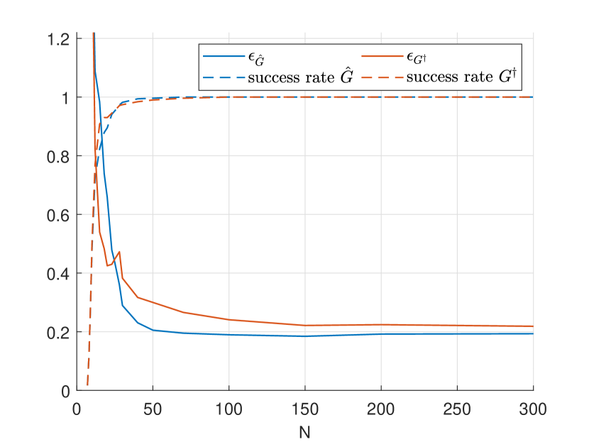
Figure 1: Error ratio of the robust $\mathcal{H}_{2}$-norm and the ratio of feasible SDP in Theorem 2, depending on the data length $N$, averaged over $2000$ experiments for different right inverses.

At last, we analyze the feasibility of the SDP. Fig. 1 shows the ratio of how often the SDP is feasible compared to the total number of experiments. This leads to similar results as before. For small sample sizes, the problem is rarely feasible, even though the LFT is well-posed. This is due to the $\mathcal{H}_{2}$-norm requiring asymptotic stability of the system. It becomes feasible with increasing $N$ such that an upper bound can be computed. Similarly to before, this may be explained by the trade-off between small $YG$ and small uncertainty set. However, a detailed theoretical or empirical case study is beyond the scope of this paper and is left for future research.

VI CONCLUSION

We have introduced a new LFT parametrization for the linear regression problem with error-in-variables, exploiting the Sherman-Morrison-Woodbury formula. Moreover, we demonstrated how to employ this data-driven parametrization to derive a guaranteed upper bound on the $\mathcal{H}_{2}$-norm of an unknown linear system using a finite number of noisy input-state measurements by solving an SDP. The presented framework allows to neatly incorporate many different setups, as designing controllers or input-output settings. Future research should extend this framework, for example, by reducing the size of the uncertainty introduced by measurement errors and disturbances.

References

- [1] J. Coulson, J. Lygeros, and F. Dörfler, “Data-Enabled Predictive Control: In the Shallows of the DeePC,” in 18th European Control Conference (ECC), 2019, pp. 307–312.
- [2] J. Berberich, C. W. Scherer, and F. Allgöwer, “Combining prior knowledge and data for robust controller design,” IEEE Transactions on Automatic Control, vol. 68, no. 8, pp. 4618–4633, 2023.
- [3] T. Martin, T. B. Schön, and F. Allgöwer, “Guarantees for data-driven control of nonlinear systems using semidefinite programming: A survey,” Annual Reviews in Control, vol. 56, p. 100911, 2023.
- [4] S. Oymak and N. Ozay, “Non-asymptotic Identification of LTI Systems from a Single Trajectory,” in American Control Conference (ACC), 2019, pp. 5655–5661.
- [5] A. Romer, J. Berberich, J. Köhler, and F. Allgöwer, “One-Shot Verification of Dissipativity Properties From Input–Output Data,” IEEE Control Systems Letters, vol. 3, no. 3, pp. 709–714, 2019.
- [6] H. J. van Waarde and M. Mesbahi, “Data-driven parameterizations of suboptimal LQR and H2 controllers,” IFAC-PapersOnLine, vol. 53, no. 2, pp. 4234–4239, 2020.
- [7] H. J. van Waarde, M. K. Camlibel, and M. Mesbahi, “From Noisy Data to Feedback Controllers: Nonconservative Design via a Matrix S-Lemma,” IEEE Transactions on Automatic Control, vol. 67, no. 1, pp. 162–175, 2022.
- [8] C. De Persis and P. Tesi, “Formulas for data-driven control: Stabilization, optimality, and robustness,” IEEE Transactions on Automatic Control, vol. 65, no. 3, pp. 909–924, 2020.
- [9] J. Berberich, A. Romer, C. W. Scherer, and F. Allgöwer, “Robust data-driven state-feedback design,” in Proc. American Control Conference, 2020, pp. 1532-1538, Jul. 2019.
- [10] H. J. van Waarde, J. Eising, H. L. Trentelman, and M. K. Camlibel, “Data Informativity: A New Perspective on Data-Driven Analysis and Control,” IEEE Transactions on Automatic Control, vol. 65, no. 11, pp. 4753–4768, 2020.
- [11] A. Koch, J. Berberich, and F. Allgöwer, “Verifying dissipativity properties from noise-corrupted input-state data,” in 2020 59th IEEE Conference on Decision and Control (CDC), 2020, pp. 616–621.
- [12] T. Söderström, “Why are errors-in-variables problems often tricky?” in 2003 European Control Conference (ECC), 2003, pp. 802–807.
- [13] V. Cerone, V. Razza, and D. Regruto, “Set-membership errors-in-variables identification of mimo linear systems,” Automatica, vol. 90, pp. 25–37, 2018.
- [14] J. Miller, T. Dai, and M. Sznaier, “Data-Driven Stabilizing and Robust Control of Discrete-Time Linear Systems with Error in Variables,” Tech. Rep., 2023.
- [15] J. Berberich, J. Köhler, M. A. Müller, and F. Allgöwer, “Stability in data-driven MPC: an inherent robustness perspective,” in 61st Conference on Decision and Control (CDC), 2022, pp. 1105–1110.
- [16] A. Bisoffi, L. Li, C. De Persis, and N. Monshizadeh, “Controller synthesis for input-state data with measurement errors,” Tech. Rep., 2024.
- [17] J. Sherman and W. J. Morrison, “Adjustment of an Inverse Matrix Corresponding to a Change in One Element of a Given Matrix,” The Annals of Mathematical Statistics, vol. 21, no. 1, pp. 124–127, 1950.
- [18] M. A. Woodbury, Inverting modified matrices, ser. SRG Memorandum report ; 42, Princeton University, Ed. Princeton, NJ: Department of Statistics, Princeton University, 1950.
- [19] C. W. Scherer, “Robust Mixed Control and Linear Parameter-Varying Control with Full Block Scalings,” in Advances in Linear Matrix Inequality Methods in Control, 2000, pp. 187–207.
- [20] S. Weiland and C. Scherer, “Linear Matrix Inequality in Control,” 2000.
- [21] R. Strasser, J. Berberich, and F. Allgower, “Data-driven control of nonlinear systems: Beyond polynomial dynamics,” in 2021 60th IEEE Conference on Decision and Control (CDC). IEEE, Dec. 2021.
- [22] M. S. Sadabadi and D. Peaucelle, “From static output feedback to structured robust static output feedback: A survey,” Annual Reviews in Control, vol. 42, pp. 11–26, Jan. 2016.
- [23] F. Brändle and F. Allgöwer, “A system parameterization for direct data-driven estimator synthesis,” Oct. 2024.
- [24] R. Penrose, “On best approximate solutions of linear matrix equations,” Mathematical Proceedings of the Cambridge Philosophical Society, vol. 52, no. 1, pp. 17–19, 1956.
- [25] J. C. Willems, P. Rapisarda, I. Markovsky, and B. L. M. De Moor, “A note on persistency of excitation,” Systems & Control Letters, vol. 54, no. 4, pp. 325–329, 2005.