IFJPAN-IV-2024-12

Pseudo-observables and Deep Neural Network for mixed CP $H\to\tau\tau$ decays at LHC.

E. Richter-Was^a, T. Yerniyazov^b and Z. Was^c

^a Institute of Physics, Jagiellonian University, Łojasiewicza 11, 30-348 Kraków, Poland

^b Faculty of Physics, Astronomy and Applied Computer Science, Jagiellonian University, Łojasiewicza 11, 30-348 Kraków, Poland

^c Institute of Nuclear Physics, IFJ-PAN, Radzikowskiego 152, 31-342 Kraków, Poland

ABSTRACT

The consecutive steps of cascade decay initiated by $H\to\tau\tau$ can be useful for the measurement of Higgs couplings and in particular of the Higgs boson parity. The standard analysis method applied so far by ATLAS and CMS Collaborations was to fit a one-dimensional distribution of the angle between reconstructed decay planes of the $\tau$ lepton decays, $\phi^{*}$, which is sensitive to transverse spin correlations of the $\tau$ decays and, hence, to the CP state mixing angle, $\phi^{CP}$.

Machine Learning techniques (ML) offer opportunities to manage such complex multidimensional signatures. The multidimensional signatures, the 4-momenta of the $\tau$ decay products can be used directly as input information to the machine learning algorithms to predict the CP-sensitive pseudo-observables and/or provide discrimination between different CP hypotheses. In the previous papers, we have shown that multidimensional signatures, the 4-momenta of the $\tau$ decay products can be used as input information to the machine learning algorithms to predict the CP-sensitive pseudo-observables and/or provide discrimination between different CP hypotheses.

In this paper we show how the classification or regression methods can be used to train an ML model to predict the spin weight sensitive to the CP state of the decaying Higgs boson, parameters of the functional form of the spin weight, or the most preferred CP mixing angle of the analysed sample. The one-dimensional distribution of the predicted spin weight or the most preferred CP mixing angle of the experimental data can be examined further, with the statistical methods, to derive the measurement of the CP mixing state of the Higgs signal events in decay $H\to\tau\tau$.

This paper extends studies presented in our previous publication, with more experimentally realistic scenarios for the features lists and further development of strategies how proposed pseudo-observables can be used in the measurement.

IFJPAN-IV-2024-12

November 2024

T. Y. was supported in part by grant No. 2019/34/E/ST2/00457 of the National Science Center (NCN), Poland and also by the Priority Research Area Digiworld under the program Excellence Initiative Research University at the Jagiellonian University in Cracow.

The majority of the numerical calculations were performed at the PLGrid Infrastructure of the Academic Computer Centre CYFRONET AGH in Kraków, Poland.

1 Introduction

Machine learning techniques are more and more often being applied in high-energy physics data analysis. With Tevatron and LHC experiments, they became an analysis standard. For the recent reviews see e.g. [1, 2, 3].

In this paper, we present how ML techniques can help exploit the substructure of the hadronically decaying $\tau$ leptons in the measurement of the Higgs boson CP-state mixing angle $\phi^{CP}$ in $H\to\tau\tau$ decay. This problem has a long history [4, 5], and was studied both for electron-positron [6, 7] and for hadron-hadron [8, 9] colliders. Following the proposed by those papers one-dimensional observable, a polar angle $\phi^{*}$ between $\tau$ leptons decay planes, ATLAS and CMS Collaborations measured the CP mixing angle $\phi^{CP}$ with Run 2 data collected in pp collisions at LHC. The Standard Model (SM) predicts that the scalar Higgs boson is in the $\phi^{CP}=0^{\circ}$ state while the pseudo-scalar would be in the $\phi^{CP}=90^{\circ}$ state for the Higgs couplings to $\tau$ pairs. The measured value by ATLAS Collaboration  [10] is $\phi^{CP}=9^{\circ}\pm 16^{\circ}$, and by CMS Collaboration  [11] $\phi^{CP}=-1^{\circ}\pm 19^{\circ}$. While data disfavour pure pseudo-scalar coupling with more than 3 standard deviations significance and are compatible with SM expectations of Higgs couplings to $\tau$ leptons being scalar-like ($\phi^{CP}$ = 0), there is still room for improvement of the precision of the measurement with more data collected during ongoing LHC Run 3 and then even 10 times more data expected with High-Lumi LHC.

The theoretical basis for the measurement is simple, the cross-section dependence on the parity mixing angle has the form of the second-order trigonometric polynomial in the $\phi^{CP}$ angle. It can be implemented in the Monte Carlo simulations as the per event spin weight $wt$, which parametrises this sensitivity, see [12] for more details. Even if the problem in its nature is multidimensional: correlations between direction and momenta of the $\tau$ lepton decay products, the ML has not been used so far for experimental analysis design. This is in part, because ML adds complexity to the data analysis and requires relatively high statistics of the signal events. Also, the ML solutions need to be evaluated for their suitability in providing estimates of systematic ambiguities.

In [13, 14] we have presented ML-based analysis on the Monte Carlo simulated events for the three channels of the $\tau$ lepton-pair decays: $\rho^{\pm}\nu_{\tau}\rho^{\mp}\nu_{\tau}$, $a_{1}^{\pm}\nu_{\tau}\rho^{\mp}\nu_{\tau}$ and $a_{1}^{\pm}\nu_{\tau}a_{1}^{\mp}\nu_{\tau}$. In those papers we limited the scope to the scalar-pseudoscalar classification case. We explored the kinematics of outgoing decay products of the $\tau$ leptons and geometry of decay vertices which can be used for reconstructing original $\tau$ lepton directions. In the following paper [15], we extended ML analysis to a measurement of the scalar-pseudoscalar mixing angle $\phi^{CP}$ of the $H\to\tau\tau$ coupling, limiting it, however, to the ideal situation where the 4-momenta of all outgoing $\tau$ decay products were known. In the experimental conditions, this is not the case, because of the two neutrinos from $\tau$ decays which cannot be measured directly.

In this paper, we extend further our research to more experimentally realistic representations of $H\to\tau\tau$ events and focus on using the per-event spin weight $wt$ as a one-dimensional pseudo-observable. We train a machine learning model to predict those weights and relay on for further statistical analysis to infer the $\phi^{CP}$ mixing angle from predicted distribution. This pseudo-observable can be used as an alternative or complementary to the angle $\phi^{*}$ between $\tau$ lepton decay planes. As in [15] we still constrain ourselves to the measurement of the coupling in the most promising decay channel $H\to\tau^{+}\tau^{-}\to\rho^{+}\nu_{\tau}\rho^{-}\nu_{\tau}\to\pi^{+}\pi^{0}\nu_{\tau}\pi^{-}\pi^{0}\nu_{\tau}$.

We analyse potential solutions using deep learning algorithms [16] and a Deep Neural Network (DNN) implemented in the Tensorflow environment [17], previously found effective for binary classification [13, 14] between scalar and pseudoscalar Higgs boson hypotheses.

We employ the same DNN architecture used for multiclass classification and regression in [15]. The DNN is tasked with predicting per-event:

• Spin weight as a function of the CP mixing angle $\phi^{CP}$.

• Decay configuration dependent coefficients, for the functional form of the spin weight distribution as a function of the mixing angle $\phi^{CP}$.

• The most preferred mixing angle, i.e. the value from which the spin weight reaches its maximum.

These goals are complementary or even to a great extent redundant, e.g. with the functional form of the spin weight. We can easily find the mixing angle at which it has a maximum. However, the precision of predicting that value may not be the same for different methods. All three cases are examined as classification and regression problems.

The paper is organised as follows: Section 2 describes the basic phenomenology of the problem. Properties of the matrix elements are discussed and the notation used is introduced. In Section 3 we review feature sets (lists of variables) used as an input to the DNN and present samples prepared for analyses. Section 4 outlines ML methods and the performance of the DNN. Section 5 delves deeper into the performance across the feature sets with varying levels of realism. Section 6 presents the final discussion on pseudo-observables resulting from the trained DNN and prospects for using them for experimental measurement. Section 7 (Summary) closes the paper.

In Appendix A more technical details on the DNN architecture are given, and input data formulation for classification and regression cases is explained. We also collect figures monitoring the performance of DNN training.

2 Physics description of the problem

The most general Higgs boson Yukawa coupling to a $\tau$ lepton pair, expressed with the help of the scalar–pseudoscalar parity mixing angle $\phi^{CP}$ reads as

$${\cal L}_{Y}=N\;\bar{\tau}{\mathrm{h}}(\cos\phi^{CP}+i\sin\phi^{CP}\gamma_{5})\tau,$$ (1)

where $N$ denotes normalisation, $\mathrm{h}$ Higgs field and $\bar{\tau}$, $\tau$ spinors of the $\tau^{+}$ and $\tau^{-}$. As we will see later, this simple analytic form translates itself into useful properties of observable distributions convenient for our goal of determining $\phi^{CP}$. Recalling these definitions is therefore justified, aiding in the systematisation of observable quantity (feature) properties and correlations.

The squared matrix element for the scalar/pseudoscalar/mixed parity Higgs, decaying into $\tau^{+}\tau^{-}$ pairs can be expressed as

$$|M|^{2}\sim 1+h_{+}^{i}h_{-}^{j}R_{i,j};\;\;\;\;\;i,j=\{x,y,z\}$$ (2)

where $h_{\pm}$ denote polarimetric vectors of $\tau$ decays (solely defined by $\tau$ decay matrix elements) and $R_{i,j}$ is the density matrix of the $\tau$ lepton pair spin state. Details of the frames used for $R_{i,j}$ and $h_{\pm}$ definition are given in Ref. [18]. The corresponding CP-sensitive spin weight $wt$ has the form:

$$wt=1-h_{{+}}^{z}h_{{-}}^{z}+h_{{+}}^{\perp}R(2\phi^{CP})~{}h_{{-}}^{\perp}.$$ (3)

The formula is valid for $h_{\pm}$ defined in $\tau^{\pm}$ rest-frames, $h^{z}$ stands for longitudinal and $h^{\perp}$ for transverse components of $h$. The $R(2\phi^{CP})$ denotes the $2\phi^{CP}$ angle rotation matrix around the $z$ direction: $R_{xx}=R_{yy}={\cos 2\phi^{CP}}$, $R_{xy}=-R_{yx}={\sin 2\phi^{CP}}$. The $\tau^{\pm}$ decay polarimetric vectors $h_{+}^{i}$, $h_{-}^{j}$, in the case of $\tau^{\pm}\to\pi^{\pm}\pi^{0}\nu$ decay, read

$$h^{i}_{\pm}={\cal N}\Bigl{(}2(q\cdot p_{\nu})q^{i}-q^{2}p_{\nu}^{i}\Bigr{)},\;\;\;$$ (4)

where $\tau$ decay products $\pi^{\pm}$, $\pi^{0}$ and $\nu_{\tau}$ 4-momenta are denoted respectively as $p_{\pi^{\pm}}$, $p_{\pi^{0}},p_{\nu}$ and $q=p_{\pi^{\pm}}-p_{\pi^{0}}$. Obviously, complete CP sensitivity can be extracted only if $p_{\nu}$ is known.

Note that the spin weight $wt$ is a simple first-order trigonometric polynomial in a $2\phi^{CP}$ angle. This observation is valid for all $\tau$ decay channels. For the clarity of the discussion on the DNN results, we introduce $\alpha^{CP}=2\phi^{CP}$, which spans over $(0,2\pi)$ range. $\alpha^{CP}=0,2\pi$ corresponds to the scalar state, while $\alpha^{CP}=\pi$ corresponds to the pseudoscalar one. The spin weight can be expressed as

$$wt=C_{0}+C_{1}\cdot\cos(\alpha^{CP})+C_{2}\cdot\sin(\alpha^{CP}),$$ (5)

where coefficients

$$C_{0} = 1-h_{+}^{z}h_{-}^{z},$$

$$C_{1} = -h_{+}^{x}h_{-}^{x}+h_{+}^{y}h_{-}^{y},$$ (6)

$$C_{2} = -h_{+}^{x}h_{-}^{y}-h_{+}^{y}h_{-}^{x},$$

depend on the $\tau$ decays only. Distribution of the $C_{0},C_{1},C_{2}$ coefficients, for the sample of $H\to\tau\tau$ events used for our numerical results is shown in Figure 1. The $C_{0}$ spans $(0,2)$ range, while $C_{1}$ and $C_{2}$ of (-1, 1) range have a similar shape, quite different than the one of $C_{0}$.

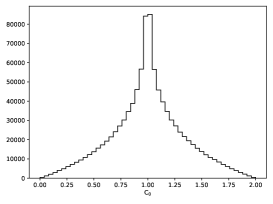
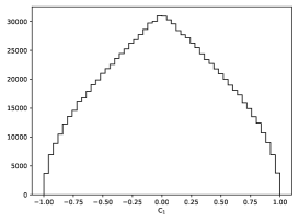
Figure 1: Distributions of the $C_{0},C_{1},C_{2}$ coefficients of formula (5), for the $H\to\tau\tau$ events sample.

The amplitude of the spin weight $wt$ as a function of $\alpha^{CP}$ depends on the multiplication of the length of the transverse components of the polarimetric vectors. The longitudinal component $h_{+}^{z}h_{-}^{z}$ defines shift with respect to zero of the $wt$ mean value and is constant over a full $(0,2\pi)$ range of $\alpha^{CP}$. The $wt$ distribution maximum is reached for $\alpha^{CP}$ = $\measuredangle(h_{+}^{T},h_{-}^{T})$, the opening angle of the transverse components of the polarimetric vectors.

The spin weight $wt$ of the formula (5) can be used to introduce transverse spin effects into the event sample when for the generation transverse spin effects were not taken into account at all. The above statement holds true regardless of whether longitudinal spin effects were included and which $\tau$ decay channels complete cascade of $H\to\tau\tau$ decay. The shape of weight dependence on the Higgs coupling to the $\tau$ parity mixing angle is preserved.

In Fig. 2 we show the distribution of the spin weight $wt$ for five example $H\to\tau\tau$ events. For each event, a single value of $\alpha^{CP}$ is the most preferred (corresponding to the largest weight), determined by its polarimetric vectors.

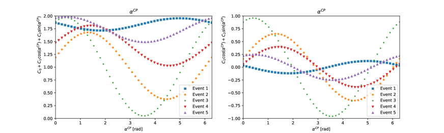
Figure 2: The spin weight $wt$ (left plot) and only its $\alpha^{CP}$ dependent component (right plot) for a few $H\to\tau\tau$ events. Note the vertical scale difference between the plots due the inclusion of the $C_{0}$ term in the left plot and its absence in the right.

3 Monte Carlo samples and feature sets

For compatibility with our previous publications [13, 14, 15], we use the same samples of generated events, namely Monte Carlo events of the Standard Model, 125 GeV Higgs boson, produced in pp collision at 13 TeV centre-of-mass energy, generated with Pythia 8.2 [20], with $\tau$ leptons decays simulated with the Tauolapp library [21]. Samples are generated without spin correlations included, each $\tau$ lepton is decayed independently.

The spin effects are introduced with the spin weight $wt$ calculated with the TauSpinner [22, 12, 23] package, for several different hypotheses of the CP mixing angle $\alpha^{CP}_{i}$ and stored together with information on $\tau$ leptons decay products. The spin weight (3), is calculated using $R_{i,j}$ density matrix and polarimetric vectors $h_{\pm}$, as explained in the previous Section. In the process of the analysis, for a given event it is possible to restore the information of the per-event coefficients $C_{0},C_{1},C_{2}$, using its value of the spin weight $wt$ at three $\alpha^{CP}$ hypotheses and solving the linear equation (5) or fitting the  (5) formula.

In this paper we present results for the case when both $\tau$ decays $\tau^{\pm}\to\rho^{\pm}\nu_{\tau}$ and about $10^{6}$ simulated Higgs events are used. To partly emulate detector conditions, a minimal set of cuts is used. We require that the transverse momenta of the visible decay products combined, for each $\tau$, are larger than 20 GeV. It is also required that the transverse momentum of each $\pi^{\pm}$ is larger than 1 GeV.

The emphasis of the paper is to explore the feasibility to learn spin weight $wt$ or its components $C_{0},C_{1},C_{2}$ with ML techniques. For the ML training as feature sets (quantities) we consider few scenarios introduced in paper [14]. We discuss the case of an idealistic benchmark scenario with the Variant-All feature set, where the four-momenta of all decay products of $\tau$ leptons are defined in the rest frame of intermediate resonance pairs ($\rho-\rho$ system). Scenarios which are more realistic in experimental conditions rely on the information that could be reconstructed from experimental data. The first one, Variant-1.1, is based on the 4-vectors and their products for visible decay products only. The second one, Variant-4.1, includes some approximate information on the original $\tau$ lepton direction.

Table 1 details the feature sets of the considered models. For more details on the specific frames and approximations used for representing neutrinos or $\tau$ lepton 4-momenta, please refer to [14]. We do not introduce any additional energy or momentum smearing, leaving the evaluation of its impact to experimental analysis.

Table 1: The feature sets used as inputs to ML algorithms, categorised by Variant-X.Y family. The third column number indicates the number of features for the $\rho^{\pm}-\rho^{\mp}$. All 4-vectors components are calculated in the rest frame of the hadronic decay products.

Notation	Features	Counts	Comments
Variant-All	4-vectors ($\pi^{\pm},\pi^{0},\nu$)	24
Variant-1.1	4-vectors ($\pi^{\pm},\pi^{0},\rho^{\pm}$), $m_{i}^{2},m_{k}^{2},y_{i},y_{k},\phi^{*}_{i,k}$	29
Variant-4.1	4-vectors ($\pi^{\pm},\pi^{0}$), 4-vectors $\tau$	24	Approx.$p_{\tau}$

4 Training and evaluation: Variant-All

We start by discussing results for an idealistic case, i.e. the Variant-All feature set. This reminds us to a great extent what was previously reported in the scope of [15].

4.1 Learning spin weights $wt$

The DNN classifier is trained on a per-event feature set to predict an $N_{class}$-dimensional per-event vector of spin weights normalised to probability. Each component of the $wt^{norm}(\alpha^{CP})$ vector is a weight associated with a discrete value of the mixing angle $\alpha^{CP}_{i}$. $N_{class}$ represents the number of discrete points into which the range $(0,2\pi)$ is divided. To guarantee that $\alpha^{CP}$ values of $0$, $\pi$ and $2\pi$ (corresponding to scalar, pseudoscalar, and again scalar states, respectively) are always included as distinct classes, the total number of classes, $N_{class}$, is maintained as an odd number. As baseline, the DNN is trained with $N_{class}$ set to 51.

Similarly, in the regression case, the DNN is trained on per-event feature sets with the corresponding spin weight vector, $wt_{i}$, for discrete $\alpha^{CP}$ values as the target variable. The DNN learns both shape and normalisation of the $wt$ vector during the training.

We quantify the DNN performance using physics-relevant criteria. The primary metric is the ability of the DNN to reproduce the per-event spin weight, $wt^{norm}$. Figure 3 illustrates the true and predicted $wt^{norm}$ distributions for two example events as a function of the class index $i$ (representing the discretised mixing parameter $\alpha^{CP}_{i}$). The blue line indicates true spin weights, while the orange line represents weights predicted by the DNN classifier. Generally, the DNN accurately predicts the spin weight for some events, but struggles for others. Encouragingly, the predicted weights exhibit the expected smooth, linear combination of $\cos(\alpha^{CP})$ and $\sin(\alpha^{CP})$. This is notable given that the loss function does not explicitly correlate nearby classes, indicating the capacity of the DNN to learn this pattern during training.

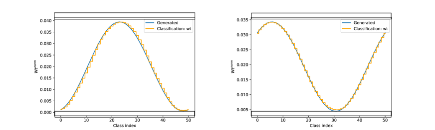
Figure 3: Normalised spin weight, $wt^{norm}$, predicted (orange line) and true (blue line), as a function of the class index for two example events. The DNN was trained using the classification method with $N_{class}$ = 51 and Variant-All.

The second criterion is the difference between the most probable predicted class and the most probable true class, denoted as $\Delta_{class}$. When calculating the difference between class indices, the periodicity of the functional form (Equation (5)) is considered. Class indices represent discrete values of $\alpha^{CP}$ within the range $(0,2\pi)$. The distance between the first and the last class is zero. We compute the distance corresponding to the smaller angle difference and assign a sign based on the clockwise orientation relative to the class index where the true $wt$ reaches its maximum.

From a physics perspective, learning the shape of the $wt$ distribution as a function of $\alpha^{CP}$ is equivalent to learning the components of the polarimetric vectors. Note Ref. [24] for the possible extension of the methods for other $\tau$ decay channels. For learning the polarimetric vectors the much larger $Z\to\tau\tau$ sample can be used too.

However, since only the shape, not the normalisation, is available, the $C_{i}$ coefficients cannot be fully recovered from $wt^{norm}$. This is not the primary goal, though. The physics interest lies in determining the preferred $\alpha^{CP}$ value for events in the analysed sample, i.e. the value where the summed $wt$ distribution reaches its maximum. This alings with the objective of potential measurement, namely, determining the CP mixing of the analysed sample, which will be discussed further in Section 6.

Figure 5, top-left panel, displays the distribution of $\Delta_{class}$ for $N_{class}$ = 51 for the DNN trained with the classification method and Variant-All/4.1/1.1. The distribution is Gaussian-like and centered around zero with standard deviation $\sigma_{\Delta_{class}}$ = 0.179 [rad] for Variant-All. The top-right panel of Figure 5 shows the distribution of $\Delta_{class}$ for $N_{class}$ = 51 using the regression method. In this case, $\sigma_{\Delta_{class}}$ = 0.170 [rad] for Variant-All. Our findings indicate that the accuracy of learning the spin weight $wt$ using classification and regression methods is comparable.

4.2 Learning $C_{0},C_{1},C_{2}$ coefficients

The second approach involves learning the $C_{0},C_{1},C_{2}$ coefficients of formula (5) for the spin weight $wt$. Once learned, these coefficients can be used to predict $wt$ and $wt^{norm}$ for a given $\alpha^{CP}$ hypothesis. The coefficients $C_{0},C_{1}$, and $C_{2}$ represent physical observables, being the products of longitudinal and transverse components of polarimetric vectors, as detailed in formulas (2).

The classification technique using the DNN is configured to learn each $C_{i}$ independently. The allowed ranges for these coefficients are well-established: $C_{0}$ spans $(0.0,2.0)$ and $C_{1},C_{2}$ span $(-1.0,1.0)$, as illustrated in Figure 1. The allowed ranges for these coefficients are divided into $N_{class}$ bins, and each event is assigned an $N_{class}$-dimensional one-hot encoded vector representing the corresponding $C_{i}$ value and serving as a label. In this setup, a single class corresponds to a specific $C_{i}$ coefficient value. During training, the DNN learns to associate per-event features with these class labels. The output is a probability distribution over the $N_{class}$ values, which is converted to a one-hot encoded representation, selecting the most probable class as the predicted $C_{i}$ value.

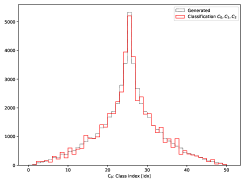
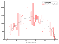
Figure 4: Distributions of true and predicted $C0,C1$, and $C2$ coefficients from formula (2). The DNN was trained using the classification method with $N_{class}$ = 51 and Variant-All.

The regression method learns all three $C_{0},C_{1}$, and $C_{2}$ coefficients simultaneously. The learning accuracy is comparable to that of the classification method.

We utilise the true and predicted $C_{0},C_{1}$, and $C_{2}$ coefficients to compute the $wt$ distribution according to formula (5). This distribution is then discretised into $N_{class}$ points (potentially different from the $N_{class}$ used for learning coefficients), and the $\alpha^{CP}_{max}$ is determined based on the class with the maximum weight. The difference between the true and predicted $\alpha^{CP}_{max}$ is shown in the middle row of Figure 5 for $N_{class}$ = 51, comparing classification (left) and regression (right) methods. The Gaussian-like shape of these distributions, centered around zero, clearly demonstrates successful method performance for Variant-All. The mean and standard deviation of these distributions are close to those obtained with the Classification:wt approach.

4.3 Learning the ${{\alpha}^{CP}_{max}}$

The third approach is to learn the per-event most preferred mixing angle, $\alpha^{CP}_{max}$, directly. For classification, the allowed range $(0,2\pi)$ is again divided into $N_{class}$ bins, where each bin represents a discrete $\alpha^{CP}$ value. A one-hot encoded $N_{class}$-dimensional vector, indicating the true $\alpha^{CP}$ value for each event, serves as the training label. The DNN outputs an $N_{class}$-dimensional probability vector, from which the class with the highest probability is selected as the predicted $\alpha^{CP}_{max}$. Notably, this approach bypasses the prediction of the spin weight or $C_{i}$ coefficients. The regression method implementation allows us to learn the per-event most preferred mixing angle, $\alpha^{CP}_{max}$, as a continuous value without having to deal with discretised predictions.

The difference between the true and predicted $\alpha^{CP}_{max}$, denoted as $\Delta\alpha^{CP}_{max}$, is shown in the bottom plot of Figure 5 for both classification (left) and regression (right) methods. The distribution for classification is Gaussian-like with a standard deviation of 0.169 [rad] for Variant-All. Regression demonstrates worse performance.

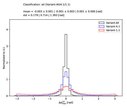
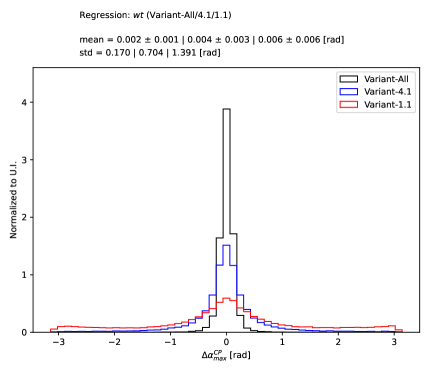
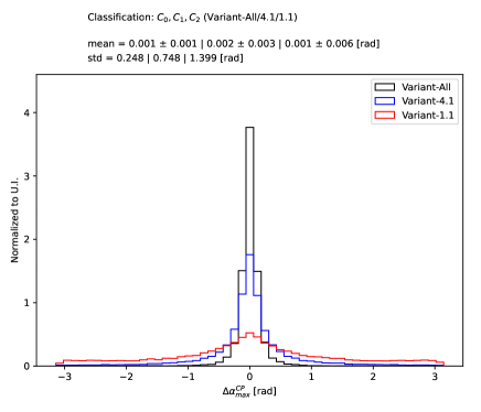
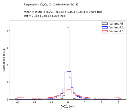
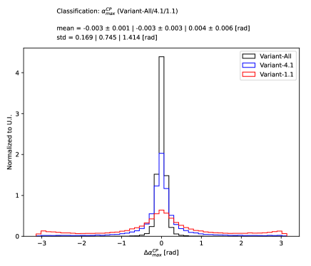
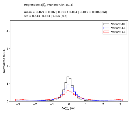
Figure 5: Distribution of the per-event difference between true and predicted $\alpha^{CP}_{max}$, obtained using: (top row) spin weight learned via classification (left) and regression (right); middle row: spin weight calculated using formula 5 and $C_{0},C_{1}$, and $C_{2}$ coefficients learned via classification (left) and regression (right); bottom row: direct comparison of true and predicted $\alpha^{CP}_{max}$ using classification (left) and regression (right). The DNN was trained with $N_{class}$ = 51 and Variant-All, Variant-4.1, Variant-1.1.

5 Training and evaluation: Variant-XX

For Variant-All, the information accessible for DNN training is identical to that used for calculating weights $wt$. Rather than employing mathematical formulas, the DNN learns to recognise patterns in the expected $wt$ values. In contrast, for other Variant-XX feature sets, while the true value for training is computed using complete event decay information, the input of the DNN is restricted. Specific details can be found in Table 1.

Table 2 compares performance on the most critical metric: the difference between the true and predicted per-event spin weight $wt$ or the true and predicted most preferred $\alpha^{CP}_{max}$ where the spin weight of the event peaks. While the information provided to the DNN is reduced gradually from Variant-4.1 to Variant-1.1, performance deteriorates.

Variant-1.1 offers sufficient information to calculate the $\alpha^{CP}$-sensitive observable $\phi^{*}$ and also includes this observable explicitly, but falls short in training the DNN to accurately learn variables directly tied to polarimetric vectors: the spin weight $wt$ and coefficients $C_{0},C_{1}$, and $C_{2}$. As shown in Equation (4), polarimetric vectors rely on neutrino directions which are experimentally undetectable. Introducing approximations for neutrino information within feature sets, as in Variant-4.1, enhances prediction accuracy.

Table 2: Mean and standard deviation of the per-event difference ($\Delta\alpha^{CP}_{max}$) between true and predicted $\alpha^{CP}_{max}$ values, obtained from DNN classification and regression methods for Variant-All, Variant-4.1, and Variant-1.1.

Method	Classification Variants: All / 4.1 / 1.1	Regression Variants: All / 4.1 / 1.1
Using $wt$	std = 0.179 / 0.714 / 1.393 [rad]	std = 0.170 / 0.704 / 1.391 [rad]
Using $C_{0},C_{1},C_{2}$	std = 0.248 / 0.748 / 1.399 [rad]	std = 0.164 / 0.681 / 1.394 [rad]
Direct	std = 0.169 / 0.745 / 1.414 [rad]	std = 0.543 / 0.883 / 1.396 [rad]

6 Results with pseudo-experiments

The experimental measurements published by ATLAS [10] and CMS [11] Collaborations rely on fitting the one-dimensional distribution of $\phi^{*}$, defined as the angle between the $\tau$ decay planes. This angle is sensitive to the transverse spin correlations between decaying $\tau$ leptons and consequently to the CP state of the Higgs boson in $H\to\tau\tau$ decays.

The calculation of $\phi^{*}$ depends on the $\tau$ lepton decay modes and was developed for hadron colliders in papers [8, 9]. It is based on the four-momenta of the visible $\tau$ decay products and, in the case of the $\tau\to\pi^{\pm}\nu$ decay, on the impact parameter of the decay vertex. The $\phi^{*}$ distribution for a sample of events with a given $\alpha^{CP}$ mixing state exhibits a characteristic first-order trigonometric polynomial shape, with the maximum value linked to an $\alpha^{CP}$ hypothesis. Following the convention used in publications, the maximum is located at $\phi^{*}=90^{\circ}$ for the scalar case and at $\phi^{*}=0^{\circ},180^{\circ}$ for the pseudoscalar case. The position of the maximum shifts according to the linear relation $\Delta\phi^{*}=2\Delta\phi^{CP}$.

Here, we employ the definition developed much earlier [5, 13], specifically tailored for $\tau\rightarrow\rho\nu$ decays. Figure 6 shows the $\phi^{*}$ distribution for events used in this analysis for three different hypotheses: $\alpha^{CP}=-29^{\circ},0^{\circ},29^{\circ}$, with the middle one corresponding to the scalar Higgs case.

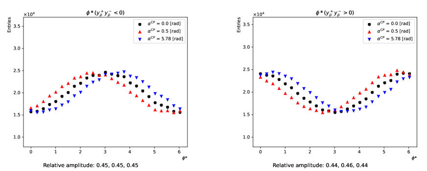
Figure 6: The $\phi^{*}$ distribution for three $\alpha^{CP}$ hypotheses, $\alpha^{CP}=-29^{\circ},0^{\circ},29^{\circ}$.

6.1 Distribution of the spin weight $wt$

In this paper, we propose an alternative or complementary observable, the spin weight $wt$ distribution, which represents the probability of an event occurring for a given $\alpha^{CP}$ hypothesis. The position of the maximum of the $wt$ distribution for a series of events indicates the $\alpha^{CP}$ mixing value for that series. As discussed in previous sections, we can train DNN algorithms on Monte Carlo events to predict the per-event spin weight $wt$ for different $\alpha^{CP}$ hypotheses. Subsequently, we can apply the trained algorithm to experimental data to predict the spin weight $wt$ and obtain its distribution within the analysed sample. Statistical analysis of this distribution (one-dimensional fit) can yield a measurement of the most probable $\alpha^{CP}$ mixing value and, consequently, the CP state of the $H\to\tau\tau$ coupling.

For the numerical ”proof of concept” presented in this paper, we used a Monte Carlo unweighting technique to isolate event series corresponding to specific $\alpha^{CP}$ hypotheses. For each series, the trained DNN predicted the per-event spin weight $wt$ as a function of different $\alpha^{CP}$ hypotheses, using either classification or regression methods. The distribution of the summed spin weights, $\Sigma wt$, served as a one-dimensional observable for measuring the most probable $\alpha^{CP}$ mixing state.

Figures 7 to 9 show, for the same unweighted event series corresponding to $\alpha^{CP}$ hypotheses with indices $idx=0,4,46$ (from the range $(0,50)$), the sum of predicted per-event spin weights $\Sigma wt$ as a function of $\alpha^{CP}$ for different feature sets. While the Variant-4.1 feature set demonstrates relatively accurate prediction of $wt$ dependence on the $\alpha^{CP}$ hypothesis, the Variant-1.1 exhibits a washed-out sensitivity to discriminate between hypotheses. Predicted per-event weights become flatter for most events shown in the left column of Figure 8, resulting in a preferred $\alpha^{CP}$ hypothesis (index $idx$ with maximum $\Sigma wt$) shifted by one. This aligns with our earlier observations on training performance for different feature sets in Section 5.

The plots in Figures 7 to 9 also reveal the relative amplitude of $\Sigma wt$, which diminishes as we move from Variant-All to Variant-1.1 due to reduced information in the input feature set.

Table 3 summarises the sensitivity of the $\Sigma wt$ observable, quantified as the amplitude in the distribution as a function of the $\alpha^{CP}$ hypothesis. Amplitude is defined as $(max-min)/((max+min)/2)$ of the $\Sigma wt$ value for a series of events with a given $\alpha^{CP}$ hypothesis.

Table 3: Amplitude of the $\Sigma wt$ distribution ($idx=4$) obtained from DNN classification and regression methods for Variant-All, Variant-4.1, and Variant-1.1.

Method	Classification Variants: All / 4.1 / 1.1	Regression Variants: All / 4.1 / 1.1
Using $wt$	44% / 35% / 12%	44% / 33% / 11%
Using $C_{0},C_{1},C_{2}$	41% / 33% / 16%	44% / 35% / 13%

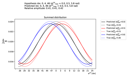
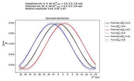
Figure 7: Summed true and predicted per-event spin weights, $\Sigma wt$, as a function of $\alpha^{CP}$ for the same series of events unweighted to $\alpha^{CP}$ hypotheses with $\alpha^{CP}=-29^{\circ},0^{\circ},29^{\circ}$. Results are shown for Classification:weights (top-left), Classification:$C_{0},C_{1},C_{2}$ (top-right), Regression:weights (bottom-left), and Regression:$C_{0},C_{1},C_{2}$ (bottom-right) methods using the Variant-All feature set for DNN training.

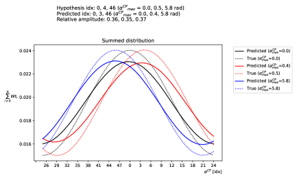
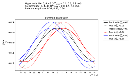
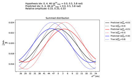
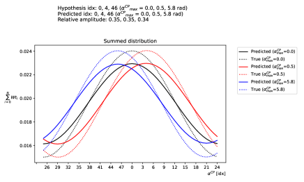
Figure 8: Summed true and predicted per-event spin weights, $\Sigma wt$, as a function of $\alpha^{CP}$ for the same series of events unweighted to $\alpha^{CP}$ hypotheses with $\alpha^{CP}=-29^{\circ},0^{\circ},29^{\circ}$. Results are shown for Classification:weights (top-left), Classification:$C_{0},C_{1},C_{2}$ (top-right), Regression:weights (bottom-left), and Regression:$C_{0},C_{1},C_{2}$ (bottom-right) methods using the Variant-4.1 feature set for DNN training.

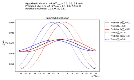
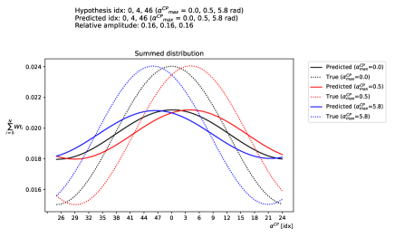
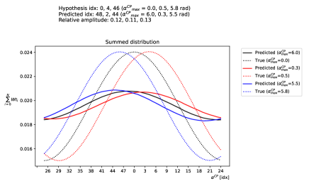
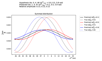
Figure 9: Summed true and predicted per-event spin weights, $\Sigma wt$, as a function of $\alpha^{CP}$ for the same series of events unweighted to $\alpha^{CP}$ hypotheses with $\alpha^{CP}=-29^{\circ},0^{\circ},29^{\circ}$. Results are shown for Classification:weights (top-left), Classification:$C_{0},C_{1},C_{2}$ (top-right), Regression:weights (bottom-left), and Regression:$C_{0},C_{1},C_{2}$ (bottom-right) methods using the Variant-1.1 feature set for DNN training.

7 Summary

We have presented a proof-of-concept study applying DNN methods to measure the Higgs boson $H\to\tau\tau$ CP-mixing angle-dependent coupling. This work extends the previous research on classifying scalar and pseudoscalar Higgs CP states (Refs. [13, 14]) and builds upon our earlier work on developing classification and regression algorithms, in which some numerical results were collected (Ref. [15]).

We have proposed using the per-event spin weight learned with DNN algorithms as a sensitive observable for measuring the Higgs boson $H\to\tau\tau$ CP-mixing angle coupling. This approach offers an alternative or complement to the commonly used $\phi^{*}$ angle, defined as the polar angle between reconstructed $\tau$ lepton decay planes. The $\phi^{*}$ angle has been used as a one-dimensional variable in recent ATLAS [10] and CMS [11] measurements, where a template fit was applied to extract the $\phi^{CP}$ value. However, it requires dedicated, per-decay mode combination algorithms to reconstruct $\phi^{*}$ angle from the kinematics of detectable $\tau$ lepton decay products. The existing algorithms might not be optimal, and their development becomes even more challenging for cascade decays involving intermediate resonances that decay into multi-body final states. Using the sum of predicted $wt$ distribution in series of events, as a function of $\alpha_{CP}$ hypothesis seems like a very interesting and promising option.

We have extended the work of [15] by investigating more realistic feature sets for the DNN training and focusing on predicting the shape of the spin weight distribution, not just the most probable $\alpha^{CP}$ mixing angle. For this ”proof-of-concept” study, we have considered only the dominant and most sensitive decay mode, $\tau\to\rho^{\pm}\nu$. We compare an idealised feature set, assuming complete knowledge of $\tau$ decay product four-momenta including neutrinos, to more realistic scenarios where only visible decay products are reconstructed or approximations are made for neutrinos or initial $\tau$ lepton momenta.

Appendix A Neural Network

A.1 Architecture

The structure of the simulated data and the DNN architecture follows what was published in our previous papers [13, 14, 15]. We use open-source libraries, TensorFlow [17] and Keras [25], to implement the models, and SciPy [26] to compute the set of $C_{i}$ coefficients while preparing data sets.

We consider the $H\to\tau\tau$ channel and both $\tau^{\pm}\to\rho^{\pm}\nu$ decays. Each data point represents an event of Higgs boson production and $\tau$ lepton pair decay products. The structure of the event is represented as follows:

$$x_{i}=(f_{i,1},...,f_{i,D}),w_{a_{i}},w_{b_{i}},...,w_{m_{i}}$$ (7)

The $f_{i,1},...,f_{i,D}$ represent numerical features, and $w_{a_{i}},w_{b_{i}},w_{m_{i}}$ are weights proportional to the likelihoods that an event comes from a class $A,B,...,M$, each representing a different $\alpha^{CP}$ mixing angle. The $\alpha^{CP}=0,2\pi$ corresponds to the scalar CP state, and $\alpha^{CP}=\pi$ corresponds to the pseudoscalar CP state. The weights calculated from the quantum field theory matrix elements are available and stored in the simulated data files. This is a convenient situation, which does not occur in many other cases of ML classification. The $A,B,...M$ distributions highly overlap in the $(f_{i,1},...,f_{i,D})$ space.

Two techniques have been used to measure the Higgs boson CP state: multiclass classification and regression:

• For multiclass classification (Figure 11), the aim is to simultaneously learn weights (probabilities) for several $\mathscr{H}_{\alpha^{CP}}$ hypotheses, learn coefficients of the weight functional form, or directly learn the mixing angle at which the spin weight has its maximum, $\alpha^{CP}_{max}$. A single class can be either a single discretised $\alpha^{CP}$ or $C_{i}$ coefficient value. The system learns the probabilities for classes to be associated with the event.

• For the regression case (Figure 11), the aim is similar to the multiclass classification case, but now the problem is defined as a continuous case. The system learns a value to be associated with the event. The value can be a vector of spin weights for a set of $\mathscr{H}_{\alpha^{CP}}$ hypotheses, a set of $C_{i}$ coefficients or $\alpha^{CP}_{max}$.

The network architecture consists of 6 hidden layers, each with 100 nodes, undergoing batch normalisation [27], followed by the ReLU activation function. Model weights are initialised randomly. We use Adam [28] as an optimiser.

The last layer is specific to the implementation case, differing in dimension of the output vector, activation function, and loss function. The details are desribed below.

Classification: The loss function used in stochastic gradient descent is the cross-entropy of valid values and neural network predictions. The loss function for a sample of $N_{evt}$ events and classification for $N_{class}$ classes reads as follows:

$$Loss=-\sum_{k=1}^{N_{evt}}\sum_{i=1}^{N_{class}}y_{i,k}ln(p_{i,k}),$$ (8)

where $k$ stands for consecutive events and $i$ for the class index. The $p_{i,k}$ represents the neural network predicted probability for event $k$ being of class $i$, while $y_{i,k}$ represents the true probability used in supervised training.

Regression: In the case of predicting $wt$, the last layer is $N$-dimensional output (the granularity with which we want to discretise it). For predicting $C_{0},C_{1},C_{2}$, the last layer is $N=3$ dimensional output, i.e. values of $C_{0},C_{1},C_{2}$. Activation of this layer is a linear function. The loss function is defined as the Mean Squared Error (MSE) between true and predicted parameters:

$$Loss=\sum_{k=1}^{N_{evt}}\sum_{i=1}^{i=N}(y_{i,k}-p_{i,k})^{2},$$ (9)

where $k$ stands for the event index and $i$ for the index of the function form parameter. The $p_{i,k}$ represents the predicted value of the $C_{i}-th$ parameter for event $k$ while $y_{i,k}$ represents the true value.

For predicting $\alpha^{CP}_{max}$, the last layer is $N=1$ dimensional output, i.e. values of $\alpha^{CP}_{max}$, with the loss function:

$$Loss=\sum_{k=1}^{N_{evt}}(1-cos(y_{k}-p_{k})),$$ (10)

where $p_{k}$ and $y_{k}$ denote the predicted and true value of $\alpha^{CP}_{max}$, respectively.

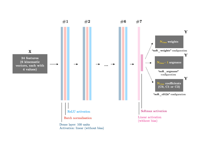
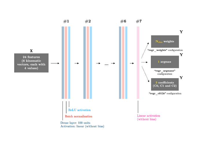
Figure 10: Architecture of classification models

Figure 11: Architecture of regression models

A.2 Training

During the training process, we monitored accuracy, the difference between predicted and true values (mean, $L_{1}$ and $L_{2}$), and training epoch relative loss function value in the case of the multiclass classification model predicting the $\alpha^{CP}_{max}$ probability distribution. For other models, training and validation loss function values were recorded.

All DNN configurations (3 multiclass classification models and 3 regression models) have been trained for 25 epochs. Extending the training process to up to 120 epochs did not lead to significant changes in the performance of the models. During the training, model weights were saved for each epoch separately, and after the training, we used the ”best” weights for evaluation. The ”best” weights were those leading to the highest validation accuracy for the multiclass classification model predicting the $\alpha^{CP}_{max}$ probability distribution or the lowest loss function value for all the other DNN configurations.

Convergence can be observed for all the configurations trained. Figure 12 shows it for models trained on the Variant-All feature set.

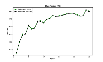
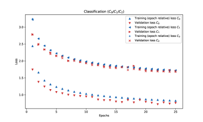
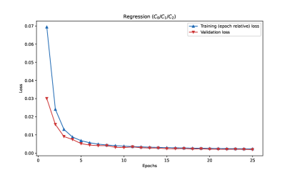
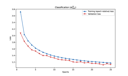
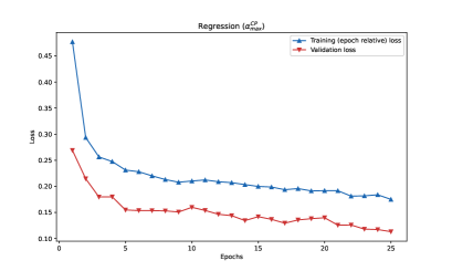
Figure 12: The DNN performance observed during the training process for Variant-All: accuracy for Classification:weights and loss for all the other models. For the classification, $N_{class}=51$ classes were used.

A.3 Unweighted events

Event weights were stored as a two-dimensional matrix, in which rows represented particular events and columns represented $\alpha^{CP}_{max}$ hypotheses. We transformed the matrix into the one containing ones and zeroes by using a Monte Carlo approach: if an element was greater than or equal to a number generated using a uniform random generator, it was replaced by $1$ or $0$, otherwise.

Therefore, each column of the unweighted events matrix contained those events that statistically represented the corresponding hypothesis. The columns were then used as a mask for filtering all the events and getting only the ones belonging to a specified $\alpha^{CP}_{max}$ hypothesis class. The fact that the summed distribution of the filtered events depicted the chosen hypothesis can be observed in Figures 7 - 9.

A.4 Negative weights

DNN models made predictions on the unweighted events, but due to the lack of restrictions in some of the configurations regarding the sign of the obtained $\alpha^{CP}_{max}$ weights, some of the predictions (up to 10%) contained negative weights. Such predictions did not have any physical interpretation, as the models were supposed to provide probabilities. We rejected those events containing negative values, ensuring they were added to the summed distribution with zero weight. Vectors containing the summed distribution were then normalised to allow us to compare predictions with true values on the same diagram.

References

- [1] Dan Guest, Kyle Cranmer and Daniel Whiteson “Deep Learning and its Application to LHC Physics”, 2018 arXiv:1806.11484 [hep-ex]
- [2] Giuseppe Carleo et al. “Machine learning and the physical sciences”, 2019 arXiv:1903.10563 [physics.comp-ph]
- [3] Kim Albertsson “Machine Learning in High Energy Physics Community White Paper”, 2018 arXiv:1807.02876 [physics.comp-ph]
- [4] M. Kramer, Johann H. Kuhn, M. L. Stong and P. M. Zerwas “Prospects of measuring the parity of Higgs particles” In Z. Phys. C64, 1994, pp. 21–30 DOI: 10.1007/BF01557231
- [5] G. R. Bower, T. Pierzchala, Z. Was and M. Worek “Measuring the Higgs boson’s parity using tau —¿ rho nu” In Phys. Lett. B543, 2002, pp. 227–234 DOI: 10.1016/S0370-2693(02)02445-0
- [6] Andre Rouge “CP violation in a light Higgs boson decay from tau-spin correlations at a linear collider” In Phys. Lett. B619, 2005, pp. 43–49 DOI: 10.1016/j.physletb.2005.05.076
- [7] K. Desch, Z. Was and M. Worek “Measuring the Higgs boson parity at a linear collider using the tau impact parameter and tau —¿ rho nu decay” In Eur. Phys. J. C29, 2003, pp. 491–496 DOI: 10.1140/epjc/s2003-01231-4
- [8] Stefan Berge and Werner Bernreuther “Determining the CP parity of Higgs bosons at the LHC in the tau to 1-prong decay channels” In Phys. Lett. B671, 2009, pp. 470–476 DOI: 10.1016/j.physletb.2008.12.065
- [9] Stefan Berge, Werner Bernreuther and Sebastian Kirchner “Prospects of constraining the Higgs boson’s CP nature in the tau decay channel at the LHC” In Phys. Rev. D92, 2015, pp. 096012 DOI: 10.1103/PhysRevD.92.096012
- [10] Georges Aad “Measurement of the CP properties of Higgs boson interactions with -leptons with the ATLAS detector” In Eur. Phys. J. C 83.7, 2023, pp. 563 DOI: 10.1140/epjc/s10052-023-11583-y
- [11] Armen Tumasyan “Analysis of the structure of the Yukawa coupling between the Higgs boson and leptons in proton-proton collisions at = 13 TeV” In JHEP 06, 2022, pp. 012 DOI: 10.1007/JHEP06(2022)012
- [12] T. Przedzinski, E. Richter-Was and Z. Was “TauSpinner: a tool for simulating CP effects in decays at LHC” In Eur. Phys. J. C74.11, 2014, pp. 3177 DOI: 10.1140/epjc/s10052-014-3177-8
- [13] R. Józefowicz, E. Richter-Was and Z. Was “Potential for optimizing the Higgs boson measurement in decays at the LHC including machine learning techniques” In Phys. Rev. D 94 American Physical Society, 2016, pp. 093001 DOI: 10.1103/PhysRevD.94.093001
- [14] K. Lasocha et al. “Machine learning classification: Case of Higgs boson state in decay at the LHC” In Phys. Rev. D 100 American Physical Society, 2019, pp. 113001 DOI: 10.1103/PhysRevD.100.113001
- [15] K. Lasocha, E. Richter-Was, M. Sadowski and Z. Was “Deep neural network application: Higgs boson state mixing angle in decay and at the LHC” In Phys. Rev. D 103 American Physical Society, 2021, pp. 036003 DOI: 10.1103/PhysRevD.103.036003
- [16] I Goodfellow, Y. Bengio and A Courville “Deep learning” MIT Press, Cambridge, MA, 2017
- [17] Martín Abadi et al. “TensorFlow: Large-Scale Machine Learning on Heterogeneous Systems” Software available from tensorflow.org, 2015 URL: https://www.tensorflow.org/
- [18] K. Desch, A. Imhof, Z. Was and M. Worek “Probing the CP nature of the Higgs boson at linear colliders with tau spin correlations: The case of mixed scalar-pseudoscalar couplings” In Phys. Lett. B579, 2004, pp. 157–164 DOI: 10.1016/j.physletb.2003.10.074
- [19] S. Jadach, Z. Was, R. Decker and Johann H. Kuhn “The tau decay library TAUOLA: Version 2.4” In Comput. Phys. Commun. 76, 1993, pp. 361–380 DOI: 10.1016/0010-4655(93)90061-G
- [20] Torbjörn Sjöstrand et al. “An introduction to PYTHIA 8.2” In Computer Physics Communications 191, 2015, pp. 159–177 DOI: https://doi.org/10.1016/j.cpc.2015.01.024
- [21] N. Davidson et al. “Universal interface of TAUOLA: Technical and physics documentation” In Computer Physics Communications 183.3, 2012, pp. 821–843 DOI: https://doi.org/10.1016/j.cpc.2011.12.009
- [22] Z. Czyczula, T. Przedzinski and Z. Was “TauSpinner Program for Studies on Spin Effect in tau Production at the LHC” In Eur.Phys.J. C72, 2012, pp. 1988 DOI: 10.1140/epjc/s10052-012-1988-z
- [23] T. Przedzinski, E. Richter-Was and Z. Was “Documentation of algorithms: program for simulating spin effects in -lepton production at LHC” In Eur. Phys. J. C79.2, 2019, pp. 91 DOI: 10.1140/epjc/s10052-018-6527-0
- [24] V. Cherepanov, E. Richter-Was and Z. Was “Monte Carlo, fitting and Machine Learning for Tau leptons” In SciPost Phys. Proc. 1, 2019, pp. 018 DOI: 10.21468/SciPostPhysProc.1.018
- [25] François Chollet “Keras”, https://keras.io, 2015
- [26] Pauli Virtanen et al. “SciPy 1.0: Fundamental Algorithms for Scientific Computing in Python” In Nature Methods 17, 2020, pp. 261–272 DOI: 10.1038/s41592-019-0686-2
- [27] Sergey Ioffe and Christian Szegedy “Batch Normalization: Accelerating Deep Network Training by Reducing Internal Covariate Shift”, 2015 eprint: arXiv:1502.03167
- [28] Diederik P. Kingma and Jimmy Ba “Adam: A Method for Stochastic Optimization”, 2014 eprint: arXiv:1412.6980