Abstract

We prove that the restriction of the vertex-reinforced jump process to a subset of the vertex set is a mixture of vertex-reinforced jump processes. A similar statement holds for the non-linear hyperbolic supersymmetric sigma model. This is then applied to vertex-reinforced jump processes on subdivided versions of graphs of bounded degree, where every edge is replaced by a finite sequence of edges. We prove that discrete-time processes associated to suitable corresponding restrictions are mixtures of positive recurrent Markov chains. We also deduce a similar statement for edge-reinforced random walks.

1 Models and Results

1.1 Motivation

One of the biggest open problems concerning vertex-reinforced jump processes, vrjp for short, is to decide whether the discrete-time process associated to vrjp on ${\mathbb{Z}}^{2}$ is a mixture of positive recurrent Markov chains for all constant initial weights. For small weights, this problem was solved by Sabot and Tarrès [ST15] and with a completely different technique by Angel, Crawford, and Kozma [ACK14]. The corresponding statement for recurrence rather than positive recurrence has been proven for all constant initial weights by Sabot in [Sab21]. Solving the above mentioned open problem seems currently out of reach. A possible approach might be the development of a renormalization group technique for vrjp on ${\mathbb{Z}}^{2}$, restricting it to smaller and smaller sublattices. We show in this paper that restriction of vrjp to subsets of a finite vertex set is a mixture of vrjp with random weights, which gives rise to a kind of renormalization flow on the distributions of these random weights. As a case study we analyze this flow on subdivided graphs, showing that it drives the effective random weights towards smaller and smaller values in a stochastic sense and thus more and more into the positive recurrent regime.

1.2 Reinforced processes

Let $G=(\Lambda,E)$ be an undirected locally finite connected graph with vertex set $\Lambda$ endowed with edge weights $W_{e}=W_{ij}>0$, $e=\{i,j\}\in E$. The vertex-reinforced jump process (vrjp) on $G$ is a continuous-time jump process $(Y_{t})_{t\geq 0}$ taking values in $\Lambda$. Conditioned on $(Y_{s})_{s\leq t}$ and $Y_{t}=i\in\Lambda$, it jumps to a neighboring vertex $j\in\Lambda$ at the rate $W_{ij}L_{j}(t)$ with $L_{j}(t)=1+\int_{0}^{t}1_{\{Y_{s}=j\}}\,ds$ being the local time at $j$ with an offset of 1. Vrjp was invented by Werner in 2000. Sabot and Tarrès [ST15] introduced the vrjp in exchangeable time scale $(Z_{t}:=Y_{D^{-1}(t)})_{t\geq 0}$ with the time change $D(t)=\sum_{i\in\Lambda}(L_{i}(t)^{2}-1)$. In this time scale, vrjp is a mixture of reversible Markov jump processes; see [ST15, Theorem 2] and [SZ19, Theorem 1].

We remark that the vrjp on infinite graphs might make infinitely many jumps in finite time, which means explosion in finite time, if the weights $W_{e}$ increase fast enough far out. However, on finite graphs, this does not occur almost surely.

For technical reasons, we encode a continuous-time jump process on $G$ by two sequences of random variables $(X_{n})_{n\in{\mathbb{N}}_{0}}$ and $(T_{n})_{n\in{\mathbb{N}}_{0}}$. The random variable $X_{n}$ takes values in $\Lambda$; it encodes the $n$-th position visited. The event $\{X_{n}=X_{n+1}\}$ may occur with positive probability. If such an event occurs, we say that the process has a self-loop. The random variable $T_{n}$ takes positive real values; it encodes the waiting time for the jump from $X_{n}$ to $X_{n+1}$. The connection of this description to a continuous-time $\Lambda$-valued jump process $(Y_{t})_{t\geq 0}$ can be described on the event $\{\sum_{n=0}^{\infty}T_{n}=\infty\}$ by $Y_{t}=X_{n}$ for $\sum_{l=0}^{n-1}T_{l}\leq t<\sum_{l=0}^{n}T_{l}$. Note that in the representation $(Y_{t})_{t\geq 0}$ the information on self-loops is lost. In the case of explosion in finite time, the sum $\sum_{n=0}^{\infty}T_{n}$ is finite. In this case, $Y_{t}$ is only defined for $t<\sum_{n=0}^{\infty}T_{n}$, but the description in terms of $X_{n},T_{n}$ still exists for all $n$. This is why we do not need any assumptions on the weights $W$ that avoid explosions in finite time.

Our first result concerns the vrjp restricted to a subset $J\subseteq\Lambda$. We define the restriction to a subset for a general continuous-time jump process.

Definition 1.1 (Removal of self-loops and restriction to a subset: process)

Let $(X_{n},T_{n})_{n\in{\mathbb{N}}_{0}}$ be a continuous-time jump process on $G$. Recursively, we take $\sigma_{0}:=0$ and for $n\in{\mathbb{N}}$, on the event $\{\sigma_{n-1}<\infty\}$, we define $\sigma_{n}:=\inf\{l>\sigma_{n-1}:X_{l}\neq X_{\sigma_{n-1}}\}$ to be the index of the next jump to a different location. The process with self-loops removed is defined by $(X^{\neq},T^{\neq})=(X^{\neq}_{n},T^{\neq}_{n})_{n\in{\mathbb{N}}_{0}}:=(X_{\sigma_{n}},\sum_{l=\sigma_{n}}^{\sigma_{n+1}-1}T_{l})_{n\in{\mathbb{N}}_{0}}$ on the event $\{\sigma_{n}<\infty\text{ for all }n\in{\mathbb{N}}\}$.

Let $\emptyset\neq J\subseteq\Lambda$. We set recursively $\tau_{0}=0$, $\tau_{n}=\inf\{l>\tau_{n-1}:X_{l}\in J\}$ for $n\in{\mathbb{N}}$. In other words, on the event $\{X_{0}\in J\}$, $\tau_{n}$ denotes the number of jumps up to the $n$-th return to $J$. The restriction of the process to $J$ is defined on the event $\{\tau_{n}<\infty\text{ for all }n\in{\mathbb{N}}\}$ by $(X^{J},T^{J})=(X_{n}^{J},T_{n}^{J})_{n\in{\mathbb{N}}_{0}}:=(X_{\tau_{n}},T_{\tau_{n}})_{n\in{\mathbb{N}}_{0}}$.

The notation $(X^{J\neq},T^{J\neq})$ means that both operations have been applied to the process $(X,T)$, first the restriction to $J$ and then self-loop removal.

One may visualize the restriction as editing a film of the continuous time representation of the jump process, cutting out all parts of the film where the jumping particle is not in $J$, but the cut locations in the edited film remain visible as self-loops. Removal of these self-loops in this edited film means that the corresponding cut locations become invisible.

Note that the definitions of $X^{\neq}$ and $X^{J}$ do not use the $T$-components of the process. In particular, the definitions of $X^{\neq}$, $X^{J}$, and $X^{J\neq}$ make also sense if one starts with a discrete-time process $(X_{n})_{n\in{\mathbb{N}}_{0}}$ only.

The mixing measure representing vrjp in exchangeable time scale as a mixture of Markov jump processes has been described in terms of a random field $\beta_{\Lambda}=(\beta_{i})_{i\in\Lambda}$ in [STZ17, Proposition 2] for finite graphs and in [SZ19, Theorem 1] for infinite graphs. Because the law $\nu^{W}_{\Lambda}$ of this random field $\beta_{\Lambda}$ appears in the present paper in an additional role, we review it first for a finite set $\Lambda$ including a pinning point $\rho\in\Lambda$. Take a symmetric matrix $W=(W_{ij})_{i,j\in\Lambda}\in[0,\infty)^{\Lambda\times\Lambda}$ of weights. Note that $W$ may have positive diagonal entries. For $\beta\in{\mathbb{R}}^{\Lambda}$, define

$$H_{\Lambda,\beta}^{W}=H_{\beta}^{W}=H_{\beta}:=2\operatorname{diag}(\beta)-W,$$ (1.1)

where $\operatorname{diag}(\beta)$ denotes the diagonal matrix with diagonal entries given by $\beta_{i}$, $i\in\Lambda$. Let $1\in{\mathbb{R}}^{\Lambda}$ denote the column vector having all entries equal to 1, which implies that the Euclidean inner product $\left\langle{1,H_{\beta}1}\right\rangle$ is the sum of all entries of the matrix $H_{\beta}$. The law of $\beta_{\Lambda}$ equals the probability measure

$$\nu^{W}_{\Lambda}(d\beta):=\left(\frac{2}{\pi}\right)^{\frac{|\Lambda|}{2}}1_{\{H_{\beta}>0\}}\frac{e^{-\frac{1}{2}\left\langle{1,H_{\beta}1}\right\rangle}}{\sqrt{\det H_{\beta}}}\,d\beta$$ (1.2)

on ${\mathbb{R}}^{\Lambda}$, where the notation $H_{\beta}>0$ means that the matrix $H_{\beta}$ is positive definite. The probability measure $\nu^{W}_{\Lambda}$ was introduced for $W_{ii}=0$ in [STZ17, Definition 1] and generalized for $W_{ii}\geq 0$ in [SZ19, Section 5.1]; see also [LW20, Section 4]. [SZ19, Proposition 1] extends the definition of $\nu^{W}_{\Lambda}$ to infinite graphs.

We use the following notation. For a vector $v\in{\mathbb{R}}^{K}$, a matrix $A\in{\mathbb{R}}^{K\times L}$, and subsets $I\subseteq K$ and $J\subseteq L$ of the index sets, we denote by $v_{I}$ the restriction of $v$ to $I$ and by $A_{IJ}$ the restriction of $A$ to $I\times J$. Let $P_{\rho}^{W,\Lambda}$ denote the law of the vrjp in exchangeable time scale on $\Lambda$ starting in $\rho$ with weights $W$.

Theorem 1.2 (Restriction of vrjp as a mixture of vrjps)

Assume that the graph $G$ is finite without self-loops and partition its vertex set $\Lambda=I\cup J$, $I\cap J=\emptyset$, with $|J|\geq 2$. Consider the vrjp $(X,T)$ in exchangeable time scale on $\Lambda$ starting at $\rho\in J$ with weights $W$. The restrictions $(X^{J},T^{J})$ and $(X^{J\neq},T^{J\neq})$ to $J$ without or with self-loops removed are mixtures of vrjps in exchangeable time scale on $J$ with random weights

$$W^{J}(\beta_{I})= (W^{J}_{ij}(\beta_{I}))_{i,j\in J}:=W_{JJ}+W_{JI}([H_{\beta}]_{II})^{-1}W_{IJ}\text{ and }$$ (1.3)

$$W^{J\neq}(\beta_{I}):= \left(W^{J}_{ij}(\beta_{I})1_{\{i\neq j\}}\right)_{i,j\in J},$$ (1.4)

respectively. They depend on a random vector $\beta_{I}\in{\mathbb{R}}^{I}$, where $\beta_{I\cup\{\rho\}}\in{\mathbb{R}}^{I\cup\{\rho\}}$ is distributed according to $\nu_{I\cup\{\rho\}}^{\widehat{W}}$ with $\widehat{W}\in{\mathbb{R}}^{(I\cup\{\rho\})\times(I\cup\{\rho\})}$ obtained by restricting the parameters $W$ to $I$ and wiring all points in $J$ at $\rho$:

$$\widehat{W}_{ij}=\widehat{W}_{ji}=\begin{cases}W_{ij}&\text{ for }i,j\in I,\\ \sum_{k\in J}W_{ik}&\text{ for }i\in I,j=\rho,\\ 0&\text{ for }i=j=\rho.\end{cases}$$ (1.5)

In the case of $(X^{J\neq},T^{J\neq})$ this means the following for any event $A\subseteq J^{{\mathbb{N}}_{0}}\times{\mathbb{R}}_{+}^{{\mathbb{N}}_{0}}$.

$$P_{\rho}^{W,\Lambda}((X^{J\neq},T^{J\neq})\in A)= \int_{{\mathbb{R}}^{I\cup\{\rho\}}}P_{\rho}^{W^{J\neq}(\beta_{I}),J}((X,T)\in A)\,\nu_{I\cup\{\rho\}}^{\widehat{W}}(d\beta_{I\cup\{\rho\}})$$

$$= \int_{{\mathbb{R}}^{\Lambda}}P_{\rho}^{W^{J\neq}(\beta_{I}),J}((X,T)\in A)\,\nu_{\Lambda}^{W}(d\beta_{\Lambda}).$$ (1.6)

The analogous statement holds for $(X^{J},T^{J})$.

Note that on the l.h.s. in (1.6) the process $(X^{J\neq},T^{J\neq})$ is built from the canonical process $(X,T)$ on $\Lambda^{{\mathbb{N}}_{0}}\times{\mathbb{R}}_{+}^{{\mathbb{N}}_{0}}$, while on the r.h.s. $(X,T)$ means the canonical process on $J^{{\mathbb{N}}_{0}}\times{\mathbb{R}}_{+}^{{\mathbb{N}}_{0}}$.

An explicit formula for the probability density of $\beta_{I}$ can be found in [SZ19, Lemma 4 combined with Lemma 5(i)]; however we do not need it here.

Comparison with the restriction property observed by Davis and Volkov.

In the special case of $J$ being a set of consecutive integers on a one-dimensional integer interval this restriction property has already been observed by Davis and Volkov in [DV02, Section 3]. In this special case, $W^{J\neq}$ is deterministic and equals the restriction of $W$ to $J\times J$. Hence, in this special case, $(X^{J\neq},T^{J\neq})$ is again a vrjp, not only a mixture of vrjps. The analogous property holds on a tree.

Subdivisions.

For $r\in{\mathbb{N}}_{0}$, we define the $2^{r}$-subdivision $G_{r}=(\Lambda_{r},E_{r})$ of the undirected graph $G=(\Lambda,E)$ to be obtained by replacing every edge in $G$ by a series of $2^{r}$ edges; see Figure 1 for an illustration. It will be convenient to have $\Lambda_{0}=\Lambda$ and $\Lambda_{l}\subseteq\Lambda_{r}$ for $l\leq r$; see also Definition 3.2 below.

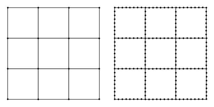
Figure 1: A part of ${\mathbb{Z}}^{2}$ on the left and its 8-subdivided version on the right.

The next result considers vrjp on a subdivided graph $G_{r}$ with random weights $W$. If the graph has degree bounded by $d$, the following result of Sabot and Tarrès allows us to deduce recurrence of the restriction to $G_{l}$ with $l<r$, provided $r-l$ is large enough depending on ${\mathbb{E}}[W_{e}^{\alpha}]$, $d$, and $\alpha$.

Fact 1.3 ([ST15, Corollary 3]; see also [ACK14, Theorem 20])

Let $d\in{\mathbb{N}}$ and $\alpha\in(0,\frac{1}{4}]$. Then, there is ${c_{1}}={c_{1}}(d,\alpha)>0$ such that for all connected undirected graphs $G=(\Lambda,E)$ with vertex degree bounded by $d$, all independent random weights $W=(W_{e})_{e\in E}$ (not necessarily identically distributed) with ${\mathbb{E}}[W_{e}^{\alpha}]\leq{c_{1}}$ for all $e\in E$, and all starting points $\rho\in\Lambda$, the discrete-time process associated to vrjp with random weights $W$ starting in $\rho$ is a mixture of positive recurrent Markov chains.

Theorem 1.4 (Vrjp on subdivided graphs)

Let $G=(\Lambda,E)$ be a connected undirected graph without self-loops and take $l,r\in{\mathbb{N}}_{0}$ with $l\leq r$. Let $(X,T)$ be vrjp in exchangeable time scale on the subdivided graph $G_{r}$ with starting point $\rho\in\Lambda$ and random weights $W_{e}>0$, $e\in E_{r}$, with respect to some probability measure with corresponding expectation ${\mathbb{E}}$. Its restriction $(X^{\Lambda_{l}\neq},T^{\Lambda_{l}\neq})$ to $\Lambda_{l}$ with self-loops removed is again a mixture of vrjps on $G_{l}$ with random weights denoted by $W^{(l)}=(W_{e}^{(l)})_{e\in E_{l}}$. If the family $W=(W_{e})_{e\in E_{r}}$ is independent or i.i.d., then so is the family $W^{(l)}$. Given $W$, the conditional law of $W^{(l)}$ can be described in terms of the restriction $\beta_{\Lambda_{r}\setminus\Lambda_{l}}$ of a $\nu_{\Lambda_{r}}^{W}$-distributed random field $\beta$. For any finite subgraph $\tilde{G}$ of $G$ and the corresponding subdivision $\tilde{G}_{l}=(\tilde{\Lambda}_{l},\tilde{E}_{l})$, the restriction of $W^{(l)}$ to $\tilde{E}_{l}$ equals $W^{\tilde{\Lambda}_{l}}$ given in (1.3) with $J=\tilde{\Lambda}_{l}$ and $I=\tilde{\Lambda}_{r}\setminus\tilde{\Lambda}_{l}$, and fulfills the recursion equations described in Lemma 3.3, below. In particular, one has

$$P_{\rho}^{W,\Lambda_{r}}((X^{\Lambda_{l}\neq},T^{\Lambda_{l}\neq})\in\cdot)=\int_{{\mathbb{R}}^{\Lambda_{r}}}P_{\rho}^{W^{(l)\neq}(\beta),\Lambda_{l}}((X,T)\in\cdot)\,\nu_{\Lambda_{r}}^{W}(d\beta).$$ (1.7)

Assume that the vertex degree of $G$ is bounded by $d$. Moreover, assume that the weights $W_{e}$, $e\in E_{r}$, are i.i.d. and satisfy ${\mathbb{E}}[W_{e}^{\alpha}]\leq{c_{1}}2^{\alpha(r-l)}$ for some $\alpha\in(0,\tfrac{1}{4}]$ with the constant ${c_{1}}(d,\alpha)$ from Fact 1.3. Then, the process $X^{\Lambda_{l}\neq}$ is a mixture of positive recurrent reversible Markov chains.

One could weaken the assumption of the recurrence statement by making only an independence assumption rather than an i.i.d. assumption. To increase readability of the proof, we only treat the stronger assumption.

Consequences for linearly edge-reinforced random walk.

Linearly edge-reinforced random walk (errw) $(X_{n})_{n\in{\mathbb{N}}_{0}}$ on $G$ starting at $\rho$ with constant initial weights $a>0$ is defined as follows. Let $X_{0}=\rho$ and let $w_{0}(e):=a$, $e\in E$, be the initial edge weights. In each time step, the random walker jumps to a neighboring vertex with probability proportional to the weight of the traversed edge. Each time an edge is traversed, its weight is increased by 1. More formally, conditioned on $(X_{m})_{m\leq n}$ and $X_{n}=i\in\Lambda$, the conditional probability of $X_{n+1}=j\in\Lambda$ is non-zero only if $\{i,j\}\in E$. It equals $w_{n}(\{i,j\})/\sum_{k\in\Lambda:\{i,k\}\in E}w_{n}(\{i,k\})$, where $w_{n}(e)=a+\sum_{m=0}^{n-1}1_{\{\{X_{m},X_{m+1}\}=e\}}$ denotes the weight of the edge $e$ at time $n$. Errw was introduced by Diaconis in 1986 in [CD86], see [Dia88]. For more history on this process, see [MR06]. It was shown in [ST15, Theorem 1], that errw is a mixture of the discrete-time process associated to vrjp with i.i.d. Gamma($a$,1)-distributed weights $W_{e}$, $e\in E$. The following result shows that under rather general conditions, errw on a subdivided graph $G_{r}$ with constant initial weights, appropriately restricted, becomes a mixture of positive recurrent Markov chains as soon as $r$ is large enough. More precisely, we prove the following statement.

Theorem 1.5 (Errw on subdivided graphs)

Let $G=(\Lambda,E)$ be a connected undirected graph without self-loops and with vertex degree bounded by $d$. For all $r\in{\mathbb{N}}_{0}$ consider the subdivided graph $G_{r}$. Let $X$ be errw on $\Lambda_{r}$ with starting point $\rho\in\Lambda$ and with constant initial weights $a>0$. Assume that $\alpha\in\left(0,\tfrac{1}{4}\right]$, $r\in{\mathbb{N}}_{0}$, and $l\in\{0,\ldots,r\}$ satisfy $\Gamma(a+\alpha)/\Gamma(a)\leq{c_{1}}(d,\alpha)2^{\alpha(r-l)}$ with ${c_{1}}$ as in Fact 1.3. Then, the restriction $X^{\Lambda_{l}\neq}$ of errw to $\Lambda_{l}$ with self-loops removed is a mixture of positive recurrent Markov chains.

In this paper, we treat $2^{r}$-subdivisions with powers of $2$ only rather than arbitrary $k$-subdivisions for $k\in{\mathbb{N}}$. This is just for notational simplicity. General $k$-subdivisions could be treated by the same method, applying the recursive restriction described in Lemma 3.3, below, not to all edges simultaneously in every recursion step, but only to some of the edges.

Comparison with previous work on errw.

[MR09, Theorem 1.1] provides a variant of Theorem 1.5 in the special case of the graph ${\mathbb{Z}}^{2}$ with nearest-neighbor edges, showing only recurrence rather than a mixture of positive recurrent Markov chains. Note that at that time, the relation between errw and vrjp, which is an essential tool in the proof of Theorem 1.5, was not known. The present paper gives a heuristic explanation why subdivisions make errw and vrjp more recurrent: the reason is that taking subdivisions and then restricting to the original graph decreases the effective weights in a stochastic sense. This is made precise in the next lemma. By a monotonicity result of Poudevigne [PA24, Theorem 1] decreasing the weights of vrjp increases the probability of vrjp being recurrent.

Theorem 1.6 (Decay of the effective weights by restriction)

Let the graph $G$ be finite and take $0\leq l\leq r$. We endow the subdivided graph $G_{r}$ with i.i.d. edge weights $W_{e}>0$, $e\in E_{r}$. Consider the family $W^{(l)}$ of corresponding random weights from Theorem 1.4, all realized on the same probability space with expectation operator ${\mathbb{E}}$. We abbreviate $C_{\alpha}:=2^{-\alpha}\Gamma(\tfrac{1}{2}-\alpha)/\sqrt{\pi}$ for $0\leq\alpha<\frac{1}{2}$ and ${c_{2}}:=\gamma+\log 2=1.27036\ldots$, where

$$\gamma=-\int_{0}^{\infty}e^{-t}\log t\,dt=0.57721\ldots$$ (1.8)

denotes the Euler Mascheroni constant. For all $\bar{e}\in E_{l}$ and $e^{\prime}\in E_{r}$, one has

$${\mathbb{E}}[(W^{(l)}_{\bar{e}})^{\alpha}] \leq(2^{-\alpha})^{r-l}{\mathbb{E}}[W_{e^{\prime}}^{\alpha}] \text{ for }\alpha\in[0,1],$$ (1.9)

$${\mathbb{E}}[(W^{(l)}_{\bar{e}})^{\alpha}] \leq\frac{1}{C_{\alpha}}\min_{m\in\{l,\ldots,r\}}\left(C_{\alpha}(2^{-\alpha})^{r-m}{\mathbb{E}}[W_{e^{\prime}}^{\alpha}]\right)^{2^{m-l}} \text{ for }\alpha\in[0,\tfrac{1}{2}),$$ (1.10)

$${\mathbb{E}}[\log W^{(l)}_{\bar{e}}] \leq\min_{m\in\{l,\ldots,r\}}2^{m-l}\left({\mathbb{E}}[\log W_{e^{\prime}}]-(r-m)\log 2+{c_{2}}\right)-{c_{2}}.$$ (1.11)

Set $m_{0}:=r-2-\lfloor\alpha^{-1}\log_{2}(C_{\alpha}{\mathbb{E}}[W_{e^{\prime}}^{\alpha}])\rfloor$ and $m_{1}:=r-2-\lfloor(\log 2)^{-1}({\mathbb{E}}[\log W_{e^{\prime}}]+{c_{2}})\rfloor$. If $m_{0}\in\{l,\ldots,r\}$, a minimizer in (1.10) is given by $m=m_{0}$. If $m_{0}<l$ or $m_{0}>r$, it is given by $m=l$ or $m=r$, respectively. The analogous statement holds for $m_{1}$ with (1.10) replaced by (1.11).

Note that for $\alpha\in[0,\frac{1}{2})$, the bound (1.10) implies the bound (1.9), using $m=l$. The proof of Theorem 1.6 is done in Section 3 and given by induction. The induction step is based on the following lemma.

Lemma 1.7 (Induction step for moments of effective weights)

Consider the setup of Theorem 1.6. For $l\in\{1,\ldots,r\}$, $\bar{e}\in E_{l-1}$, and $e^{\prime}\in E_{l}$, we have

$${\mathbb{E}}[(W^{(l-1)}_{\bar{e}})^{\alpha}]\leq 2^{-\alpha}{\mathbb{E}}[(W^{(l)}_{e^{\prime}})^{\alpha}]\quad\text{for }\alpha\in[0,1],$$ (1.12)

$${\mathbb{E}}[(W^{(l-1)}_{\bar{e}})^{\alpha}]\leq C_{\alpha}{\mathbb{E}}[(W^{(l)}_{e^{\prime}})^{\alpha}]^{2}\quad\text{for }\alpha\in[0,\tfrac{1}{2}),$$ (1.13)

$${\mathbb{E}}[\log W^{(l-1)}_{\bar{e}}]\leq\min\{{\mathbb{E}}[\log W^{(l)}_{e^{\prime}}]-\log 2,2{\mathbb{E}}[\log W^{(l)}_{e^{\prime}}]+{c_{2}}\}$$ (1.14)

with the constants $C_{\alpha}$ and ${c_{2}}$ from Theorem 1.6. For $\alpha\in[0,\frac{1}{2})$, the bound in (1.12) is stronger than the bound in (1.13) if and only if ${\mathbb{E}}[(W^{(l)}_{e^{\prime}})^{\alpha}]>2^{-\alpha}C_{\alpha}^{-1}$. Similarly, the minimum in bound (1.14) equals ${\mathbb{E}}[\log W^{(l)}_{e^{\prime}}]-\log 2$ if and only if ${\mathbb{E}}[\log W^{(l)}_{e^{\prime}}]\geq-\log 2-{c_{2}}$. Note that the expectations do not depend on the choice of $\bar{e}$ and $e^{\prime}$.

Discussion.

The iteration of the bound (1.12) gives an exponentially decreasing upper bound for ${\mathbb{E}}[(W^{(l)}_{\bar{e}})^{\alpha}]$ as a function of $r-l$, while iteration of the other bound (1.13) is only useful for small values of ${\mathbb{E}}[(W^{(l)}_{\bar{e}})^{\alpha}]$, but then gives a doubly exponentially fast decreasing bound. Thus, for $0<\alpha<\frac{1}{2}$, there is a change of regimes in these upper bounds for ${\mathbb{E}}[(W^{(l)}_{\bar{e}})^{\alpha}]$, consisting of exponential decay for the first iteration steps with a transition to doubly exponential decay for later steps. One may speculate that there might be a change of regimes for the decay of ${\mathbb{E}}[(W^{(l)}_{\bar{e}})^{\alpha}]$ as well, not just for the upper bounds.

1.3 Non-linear hyperbolic supersymmetric sigma model

Let $\Lambda$ be a finite set containing a pinning point $\rho$ and consider interactions $W=(W_{ij})_{i,j\in\Lambda}$, $W_{ij}=W_{ji}\geq 0$, such that the graph $(\Lambda,E_{+})$ with edge set $E_{+}:=\{\{i,j\}\subseteq\Lambda:W_{ij}>0\}$ is connected.

The non-linear hyperbolic supersymmetric sigma model, $H^{2|2}$-model for short, is a statistical mechanics type model involving spin variables taking values in a supermanifold called $H^{2|2}$. The spin variables have three even (= commuting) components $x,y,z$ and two odd (= anticommuting) components $\xi,\eta$ in a real Grassmann algebra $\mathcal{A}=\mathcal{A}_{0}\oplus\mathcal{A}_{1}$ with ${\mathbb{R}}\subseteq\mathcal{A}_{0}$. Here, $\mathcal{A}_{0}\ni x,y,z$ denotes the even subalgebra and $\mathcal{A}_{1}\ni\xi,\eta$ the odd subspace. More details can be found in [DSZ10], [Swa20], and [DMR22, Appendix]. To every vertex $i\in\Lambda$ linearly independently, we associate a spin variable $\sigma_{i}=(x_{i},y_{i},z_{i},\xi_{i},\eta_{i})$ subject to the constraint

$$\sigma_{i}\in H^{2|2}:= \{(x,y,z,\xi,\eta)\in\mathcal{A}_{0}^{3}\times\mathcal{A}_{1}^{2}:\,x^{2}+y^{2}-z^{2}+2\xi\eta=-1,\operatorname{body}(z)>0\}.$$ (1.15)

Here, $\operatorname{body}(z)\in{\mathbb{R}}$ is the unique real number such that $z-\operatorname{body}(z)$ is nilpotent. We endow $\mathcal{A}_{0}^{3}\times\mathcal{A}_{1}^{2}$ with the inner product

$$\left\langle{\sigma,\sigma^{\prime}}\right\rangle:=xx^{\prime}+yy^{\prime}-zz^{\prime}+\xi\eta^{\prime}-\eta\xi^{\prime}$$ (1.16)

for $\sigma=(x,y,z,\xi,\eta),\sigma^{\prime}=(x^{\prime},y^{\prime},z^{\prime},\xi^{\prime},\eta^{\prime})$. For any smooth function $f:{\mathbb{R}}^{k}\to{\mathbb{R}}$ there is an extension to a superfunction $f:\mathcal{A}_{0}^{k}\to\mathcal{A}_{0}$ constructed by a Taylor expansion in the nilpotent parts; it is denoted by the same symbol. The same holds if $f$ is defined only on an open subset $U$ of ${\mathbb{R}}^{k}$, but then the extension is only defined on the subset of $\mathcal{A}_{0}^{k}$ with bodies in $U$. In particular, on $H^{2|2}$ the component $z$ is not an independent variable, but just an abbreviation $z=\sqrt{1+x^{2}+y^{2}+2\xi\eta}$. In the $H^{2|2}$-model, the pinning point $\rho\in\Lambda$ gets constant spin $\sigma_{\rho}=o:=(0,0,1,0,0)\in H^{2|2}$ assigned to it. The superintegration form $\mathcal{D}\sigma$ on $H^{2|2}$ is defined by

$$f\mapsto\int_{H^{2|2}}\mathcal{D}\sigma f(\sigma):=\frac{1}{2\pi}\int_{{\mathbb{R}}^{2}}dx\,dy\,\partial_{\xi}\partial_{\eta}\left(\frac{1}{z}f(x,y,z,\xi,\eta)\right)$$ (1.17)

for any superfunction $f$ decaying sufficiently fast to make the integral well-defined. The $H^{2|2}$-model $\Lambda$ is given by

$$\mu^{W}_{\Lambda}(\sigma_{\Lambda}):=\mu^{W}_{\Lambda,\rho}(\sigma_{\Lambda}):=\delta_{o}(d\sigma_{\rho})\mathcal{D}\sigma_{\Lambda\setminus\{\rho\}}\,\exp\left(\frac{1}{2}\sum_{i,j\in\Lambda}W_{ij}(1+\left\langle{\sigma_{i},\sigma_{j}}\right\rangle)\right).$$ (1.18)

Here, $\delta_{o}$ denotes the Dirac measure in $o$. Note that $\mu^{W}_{\Lambda,\rho}$ depends on the choice of $\rho$ due to the constraint $\sigma_{\rho}=o$, while the law $\nu^{W}_{\Lambda}$ of the $\beta$-field does not.

The following result shows that the restriction of the $H^{2|2}$ model is a mixture of $H^{2|2}$ models.

Theorem 1.8 (Effective weights for restrictions to subsets)

Let $\Lambda=I\cup J$, $I\cap J=\emptyset$, with $|J|\geq 2$ and $\rho\in J$. Using the weights $W^{J}(\beta_{I})$ defined in (1.3) and $\widehat{W}$ obtained from $W$ by wiring all points in $J$ at $\rho$, cf. (1.5), one has

$$\int_{(H^{2|2})^{\Lambda}}\mu_{\Lambda}^{W}(\sigma_{\Lambda})f(\sigma_{J})= \int_{{\mathbb{R}}^{\Lambda}}\nu_{\Lambda}^{W}(d\beta)\int_{(H^{2|2})^{J}}\mu_{J}^{W^{J}(\beta_{I})}(\sigma_{J})f(\sigma_{J})$$

$$= \int_{{\mathbb{R}}^{I\cup\{\rho\}}}\nu_{I\cup\{\rho\}}^{\widehat{W}}(d\beta)\int_{(H^{2|2})^{J}}\mu_{J}^{W^{J}(\beta_{I})}(\sigma_{J})f(\sigma_{J})$$ (1.19)

for any superfunction $f$ on $(H^{2|2})^{J}$ which is compactly supported or decays at least sufficiently fast so that the left-hand side of (1.19) is well-defined.

How this paper is organized.

Section 2.1 deals with the restriction of Markov jump processes on finite graphs to subgraphs, the removal of self-loops, and the combination of these two operations. In Section 2.2, this is used as an ingredient to treat the same operations for vrjp, which is viewed as a mixture of Markov jump processes. In particular, Theorem 1.2 is proved there. This theory is applied to subdivided graphs in Section 3. Section 3.1 deals with a recursive description of the random weights $W^{(l)}$ introduced in Theorem 1.4. This results in a proof of Lemma 1.7 and its consequence Theorem 1.6. Section 3.2 proves the recurrence statements for vrjp and errw given in Theorems 1.4 and 1.5. We avoided using the $H^{2|2}$ model and supersymmetry in Sections 2 and 3 to make the proofs more accessible to probabilists. Alternatively, one could deduce Theorem 1.2 from the result on the $H^{2|2}$ model given in Theorem 1.8 instead of using the restriction and conditioning property of the $\beta$-field. Proofs using superspin variables are confined to Section 4, which proves Theorem 1.8. In Appendix A, we collect relevant results about the inverse Gaussian distribution. The constants $C_{\alpha}$, ${c_{1}}$, and ${c_{2}}$ keep their meaning throughout the paper.

2 Representation as a mixture

2.1 Markov jump processes

Notation.

Consider a Markov jump process $(X,T)$ on a finite connected graph $G=(\Lambda,E)$ with $|\Lambda|\geq 2$, transition rates $q=(q_{ij})_{i,j\in\Lambda}$, and starting point $\rho$. Assume in addition that it is reversible with reversible measure $\pi=(\pi_{i})_{i\in\Lambda}\in(0,\infty)^{\Lambda}$, meaning that $\pi_{i}q_{ij}=\pi_{j}q_{ji}$ for all $i,j\in\Lambda$. The corresponding discrete-time process $X$ is a reversible Markovian random walk on the graph $G$ with edge weights, also called conductances, given by $C_{ij}=C_{ji}=\pi_{i}q_{ij}$. We assume that $C_{ij}>0$ whenever $\{i,j\}\in E$. In this context, the law of the Markov jump process together with its reversible measure is equivalently parametrized by the conductance matrix $C=(C_{ij})_{i,j\in\Lambda}$ and $\pi$ instead of $q$ and $\pi$. In the following, we realize $(X,T)$ as canonical process and denote its law by $Q^{C,\Lambda}_{\rho,\pi}$, where $\rho$ denotes the starting point. For $i\in\Lambda$, we denote the corresponding total transition rate and total weight, respectively, by

$$q_{i}:=\sum_{k\in\Lambda}q_{ik},\quad C_{i}:=\sum_{k\in\Lambda}C_{ik}.$$ (2.1)

For $n\in{\mathbb{N}}_{0}$ and $i\in\Lambda$, given $(X_{l})_{l\leq n}$, $(T_{l})_{l\leq n-1}$, and $X_{n}=i$, the random variables $X_{n+1}$ and $T_{n}$ are conditionally independent. In particular, the conditional law of $X_{n+1}$ is specified by

$$Q^{C,\Lambda}_{\rho,\pi}(X_{n+1}=j|(X_{l})_{l\leq n},(T_{l})_{l\leq n-1},X_{n}=i)=\frac{q_{ij}}{q_{i}}=\frac{C_{ij}}{C_{i}}=:p_{ij}$$ (2.2)

for $j\in\Lambda$ and the conditional law of $T_{n}$ is exponential with parameter $q_{i}$. Note that even stronger, the process $X$ and $T_{n}$ are conditionally independent under the same condition.

When we deal only with the discrete-time process $X$, but not with the sequence of waiting times $T$, the reversible measure $\pi$ becomes irrelevant; by abuse of notation we write $Q^{C,\Lambda}_{\rho}$ instead of $Q^{C,\Lambda}_{\rho,\pi}$ in this context.

Next, we deal with the law of the process $(X^{\neq},T^{\neq})$ with self-loops removed and of the restriction $(X^{J},T^{J})$ to a vertex subset $J$ introduced in Definition 1.1. The following definition describes the corresponding parameters.

Definition 2.1 (Removal of self-loops and restriction to a subset: parameters)

We define new transition probabilities, rates, and weights as follows

$$p^{\neq}=\left(p^{\neq}_{ij}:=\frac{p_{ij}}{1-p_{ii}}1_{\{i\neq j\}}\right)_{i,j\in\Lambda},\quad q^{\neq}=(q^{\neq}_{ij}:=q_{ij}1_{\{i\neq j\}})_{i,j\in\Lambda},$$ (2.3)

$$C^{\neq}=(C^{\neq}_{ij}:=C_{ij}1_{\{i\neq j\}})_{i,j\in\Lambda},\quad C^{\neq}_{i}:=\sum_{k\in\Lambda}C^{\neq}_{ik},i\in\Lambda.$$ (2.4)

For any subset $J\subseteq\Lambda$ with $\rho\in J$, $|J|\geq 2$, we set $I=\Lambda\setminus J$ and define

$$p^{J}=(p^{J}_{ij})_{i,j\in J}:=p_{JJ}+\sum_{l=0}^{\infty}p_{JI}p_{II}^{l}p_{IJ},$$ (2.5)

which is a convergent series with $p_{ij}^{J}=Q^{C,\Lambda}_{i}(X^{J}_{1}=j)$. Furthermore, we define

$$C^{J}=(C^{J}_{ij}:=C_{i}p^{J}_{ij})_{i,j\in J},\quad q^{J}=\left(q^{J}_{ij}:=\frac{C_{i}}{\pi_{i}}p^{J}_{ij}\right)_{i,j\in J}.$$ (2.6)

The notation $p^{J\neq}$, $q^{J\neq}$, and $C^{J\neq}$ means that the two operations $\mbox{}^{J}$ and $\mbox{}^{\neq}$ have been applied successively.

The next lemma shows that the just defined quantities indeed parametrize the laws of the processes $(X^{\neq},T^{\neq})$, $(X^{J},T^{J})$, and $(X^{J\neq},T^{J\neq})$.

Lemma 2.2 (Laws of removal of self-loops and restriction to a subset)

Consider a reversible Markov jump process $(X,T)$ on the finite graph $G$. Assume that it starts in $\rho\in J$, has the reversible measure $\pi$ with $\pi_{i}>0$ for all $i\in\Lambda$, and that the jump rates are given by $q_{ij}=C_{ij}/\pi_{i}$ for $i,j\in\Lambda$. Then, the processes $(X^{\neq},T^{\neq})$ and $(X^{J},T^{J})$ are again reversible Markov jump processes with rates $q^{\neq}$ and $q^{J}$, weights $C^{\neq}$ and $C^{J}$, transition probabilities $p^{\neq}$ and $p^{J}$, and reversible measures $\pi$ and $\pi|_{J}$, respectively. Applying both transformations successively, $(X^{J\neq},T^{J\neq})$ is also a reversible Markov jump process with rates $q^{J\neq}$, weights $C^{J\neq}$, transition probabilities $p^{J\neq}$, and reversible measure $\pi|_{J}$. In particular, the restriction $X^{J\neq}$ of $X$ to $J$ with self-loops removed with starting point $X_{0}=\rho\in J$ has the same law as a random walk on the complete graph over $J$ endowed with the weights $C^{J\neq}$. In other words, $Q_{\rho}^{C,\Lambda}(X^{J\neq}\in\cdot)=Q_{\rho}^{C^{J\neq},J}$.

Proof. Consider the filtration ${\mathcal{F}}_{n}=\sigma((X_{l})_{l\leq n},(T_{l})_{l\leq n-1})$, $n\in{\mathbb{N}}_{0}$. When $(X,T)$ is replaced by $(X^{\neq},T^{\neq})$ and $(X^{J},T^{J})$, the corresponding filtrations are denoted by $({\mathcal{F}}_{n}^{\neq})_{n}$ and $({\mathcal{F}}_{n}^{J})_{n}$, respectively.

We treat the process $(X^{J},T^{J})$ first. Fix $m,n\in{\mathbb{N}}_{0}$ and $i\in J$. Let $B^{J}_{n,m}:=\{X_{n}^{J}=i,\tau_{n}=m\}$. Observe that on $B^{J}_{n,m}$, one has $X_{m}=i$ and $T_{n}^{J}=T_{m}$ and that given ${\mathcal{F}}_{m}$, the process $X$ and $T_{n}^{J}$ are conditionally independent. Hence, conditionally on the same, $X^{J}_{n+1}$ and $T_{n}^{J}$ are independent. Moreover, still under the same conditions, $T_{n}^{J}=T_{m}$ is exponentially distributed with parameter $q_{i}=\sum_{k\in\Lambda}q_{ik}$ and for any $j\in J$, the event that $X_{n+1}^{J}=j$ holds with conditional probability $p_{ij}^{J}$. Note that every event $A\in\sigma({\mathcal{F}}_{n}^{J},B^{J}_{n,m})$ with $A\subseteq B^{J}_{n,m}$ fulfills $A\in{\mathcal{F}}_{m}$, and that $B^{J}_{n,m}\in{\mathcal{F}}_{m}$ holds. Thus, for $t\geq 0$, on the event $B^{J}_{n,m}$, one has

$$Q^{C,\Lambda}_{\rho,\pi}(X^{J}_{n+1}=j,T_{n}^{J}\geq t|{\mathcal{F}}_{n}^{J},B^{J}_{n,m})= E_{Q^{C,\Lambda}_{\rho,\pi}}[Q^{C,\Lambda}_{\rho,\pi}(X^{J}_{n+1}=j,T_{m}\geq t|{\mathcal{F}}_{m})|{\mathcal{F}}_{n}^{J},B^{J}_{n,m}]$$

$$= Q^{C,\Lambda}_{\rho,\pi}(X^{J}_{n+1}=j|{\mathcal{F}}_{n}^{J},B^{J}_{n,m})e^{-tq_{i}}.$$ (2.7)

Summing over $m\in{\mathbb{N}}_{0}$ and using the $\sigma$-field $\mathcal{B}_{n}^{J}:=\sigma(B^{J}_{n,m},m\in{\mathbb{N}}_{0})$ yields the following on the event $\{X_{n}^{J}=i\}=\bigcup_{m=0}^{\infty}B^{J}_{n,m}$:

$$Q^{C,\Lambda}_{\rho,\pi}(X^{J}_{n+1}=j,T_{n}^{J}\geq t|{\mathcal{F}}_{n}^{J},\mathcal{B}^{J}_{n})= Q^{C,\Lambda}_{\rho,\pi}(X^{J}_{n+1}=j|{\mathcal{F}}_{n}^{J},\mathcal{B}^{J}_{n})e^{-tq_{i}}.$$ (2.8)

Conditioning this on the smaller $\sigma$-field ${\mathcal{F}}_{n}^{J}$, we obtain on the event $\{X_{n}^{J}=i\}$,

$$Q^{C,\Lambda}_{\rho,\pi}(X^{J}_{n+1}=j,T_{n}^{J}\geq t|{\mathcal{F}}_{n}^{J})= Q^{C,\Lambda}_{\rho,\pi}(X^{J}_{n+1}=j|{\mathcal{F}}_{n}^{J})e^{-tq_{i}},$$ (2.9)

and we conclude that $X^{J}_{n+1}$ and $T_{n}^{J}$ are conditionally independent on the event $\{X_{n}^{J}=i\}$ given ${\mathcal{F}}_{n}^{J}$. Since the graph $G=(\Lambda,E)$ is finite and connected and $C_{ij}>0$ whenever $\{i,j\}\in E$, we find that $\sum_{k\in J}q^{J}_{ik}=\frac{C_{i}}{\pi_{i}}\sum_{k\in J}p^{J}_{ik}=\frac{C_{i}}{\pi_{i}}$ and hence $p^{J}_{ij}=\frac{\pi_{i}}{C_{i}}q^{J}_{ij}=q^{J}_{ij}/\sum_{k\in J}q^{J}_{ik}$. The weights for the restriction fulfill $C^{J}_{ij}=C_{i}p^{J}_{ij}=\pi_{i}q^{J}_{ij}$ and the reversibility condition $\pi_{i}q^{J}_{ij}=C_{i}p^{J}_{ij}=C_{j}p^{J}_{ji}=\pi_{j}q^{J}_{ji}$, which can be seen by multiplying the definition (2.5) of $p^{J}_{ij}$ by $C_{i}$ and using repeatedly the original reversibility condition $C_{k}p_{kl}=C_{l}p_{lk}$. This proves the claim for the process $(X^{J},T^{J})$.

Next, we treat the process $(X^{\neq},T^{\neq})$ in a similar way. Let $i\in\Lambda$, $m\in{\mathbb{N}}_{0}$, and set $B^{\neq}:=\{X_{n}^{\neq}=i,\sigma_{n}=m\}$. For the rest of this proof, the arguments are understood conditionally on ${\mathcal{F}}_{m}$ and $B^{\neq}$. Observe that $X_{m}=i$ and $T_{n}^{\neq}=\sum_{l=m}^{\sigma_{n+1}-1}T_{l}$. Inductively on $k\in{\mathbb{N}}$, on the event $B^{\neq}$, for any Borel set $S\subseteq{\mathbb{R}}^{k}$ and $j\in\Lambda$, it follows that

$$Q^{C,\Lambda}_{\rho,\pi}(X_{m}=\ldots=X_{m+k-1}=i,X_{m+k}=j,(T_{m},\ldots,T_{m+k-1})\in S|{\mathcal{F}}_{m})$$

$$= p_{ii}^{k-1}p_{ij}\operatorname{Exp}(q_{i})^{\times k}(S),$$ (2.10)

where $\operatorname{Exp}(q_{i})^{\times k}$ is the $k$-th power of the exponential distribution with parameter $q_{i}$. Note that only the special case $i=j$ is needed as induction hypothesis in this induction.

Take now $j\neq i$. In this case, (2.10) implies that the waiting time $T_{n}^{\neq}=\sum_{l=\sigma_{n}}^{\sigma_{n+1}-1}T_{l}$ consists of a geometrically distributed number of summands with $Q^{C,\Lambda}_{\rho,\pi}(\sigma_{n+1}-\sigma_{n}=d|{\mathcal{F}}_{m})=(1-p_{ii})p_{ii}^{d-1}$, $d\in{\mathbb{N}}$, on $B^{\neq}$. Conditioning in addition on $\sigma_{n+1}-\sigma_{n}$, the summands $T_{l}$ are conditionally i.i.d. exponentially distributed with parameter $q_{i}$. By the thinning property of the Poisson process, the waiting time $T_{n}^{\neq}$ is exponentially distributed with parameter $(1-p_{ii})q_{i}=q_{i}-q_{ii}=\sum_{k\in\Lambda}q_{ik}^{\neq}=:q_{i}^{\neq}$, where we used (2.2) for $i=j$. Summing over $k$ yields

$$Q^{C,\Lambda}_{\rho,\pi}(X_{n+1}^{\neq}=j,T_{n}^{\neq}\geq t|{\mathcal{F}}_{m})= \sum_{k=1}^{\infty}p_{ii}^{k-1}p_{ij}\operatorname{Exp}(q_{i})^{\ast k}([t,\infty))=p_{ij}^{\neq}e^{-tq_{i}^{\neq}};$$ (2.11)

here $\operatorname{Exp}(q_{i})^{\ast k}$ denotes the $k$-fold convolution of $\operatorname{Exp}(q_{i})$. Furthermore, the new transition probabilities $p^{\neq}_{ij}$ and the new transition rates $q^{\neq}_{ij}$ are related for all $i,j\in\Lambda$ by

$$\frac{q^{\neq}_{ij}}{q^{\neq}_{i}}=\frac{q_{ij}1_{\{i\neq j\}}}{(1-p_{ii})q_{i}}=\frac{p_{ij}1_{\{i\neq j\}}}{1-p_{ii}}=p^{\neq}_{ij}.$$ (2.12)

Finally, the new reversibility relation $C^{\neq}_{ij}=\pi_{i}q^{\neq}_{ij}=\pi_{j}q^{\neq}_{ji}$ is an immediate consequence of the original one.   

2.2 Application to vrjp

In the last section, the parameters $q$, $\pi$, and $C$ were deterministic. In this section, which deals with vrjp rather than Markov jump processes, they become random because vrjp in exchangeable time-scale is a mixture of reversible Markov jump processes as was shown in [ST15, Theorem 2]. The role of the deterministic conductances $C_{ij}$ is now overtaken by random conductances $W_{ij}e^{u_{i}+u_{j}}$ with appropriate random variables $u_{i}$, $i\in\Lambda$, introduced in Lemma 2.5, below. These $u$-variables are functions of the $\nu^{W}_{\Lambda}$-distributed random field $\beta$ introduced in (1.2). The following remark reviews some crucial properties of this $\beta$-field.

Remark 2.3 (Properties of $\beta$, [SZ19, Sect. 5.1, Proposition 1 and Lemma 5])

Let $\beta\sim\nu^{W}_{\Lambda}$. Then, $(\beta_{i}-\frac{1}{2}W_{ii})_{i\in\Lambda}\sim\nu^{W^{\neq}}_{\Lambda}$ with $W^{\neq}=(W^{\neq}_{ij}=W_{ij}1_{\{i\neq j\}})_{i,j\in\Lambda}$. For any $i\in\Lambda$, one has

$$(2\beta_{i}-W_{ii})^{-1}\sim\operatorname{IG}\left(W_{i}^{-1},1\right)\quad\text{with}\quad W_{i}=\sum_{j\in\Lambda\setminus\{i\}}W_{ij},$$ (2.13)

where $\operatorname{IG}(\mu,\lambda)$ denotes the inverse Gaussian distribution with parameters $\mu,\lambda>0$; see Appendix A. Assume that $\Lambda=I\cup J$ is finite with $I\cap J=\emptyset$, $|J|\geq 2$. The conditioning property states that conditioned on $\beta_{I}$, one has $\beta_{J}\sim\nu_{J}^{W^{J}(\beta_{I})}$, and hence $(\beta_{j}-\frac{1}{2}W_{jj}^{J}(\beta_{I}))_{j\in J}\sim\nu_{J}^{W^{J\neq}(\beta_{I})}$ with the weights $W^{J}$ and $W^{J\neq}$ from (1.3) and (1.4). The restriction property states that $\beta_{I}$ is the restriction of $\beta_{I\cup\{\rho\}}\sim\nu_{I\cup\{\rho\}}^{\widehat{W}}$ with $\widehat{W}$ defined in (1.5).

The next remark describes how to recover the law of the original process $(X,T)$ with self-loops from its self-loop removed version $(X^{\neq},T^{\neq})$ and additional auxiliary independent Poisson processes.

Remark 2.4 (Decoration of vrjp with self-loops)

Vrjp with self-loops described by $P_{\rho}^{W,\Lambda}$ and vrjp without self-loops described by $P_{\rho}^{W^{\neq},\Lambda}$ are related as follows. If $(X,T)$ is distributed according to $P_{\rho}^{W,\Lambda}$, then $(X^{\neq},T^{\neq})$ is distributed according to $P_{\rho}^{W^{\neq},\Lambda}$. Conversely, if $(\tilde{X},\tilde{T})$ is distributed according to $P_{\rho}^{W^{\neq},\Lambda}$, given any vertex $i\in\Lambda$, we take a Poisson process with intensity $\frac{1}{2}W_{ii}$, visualized as exponential clocks. These Poisson processes should be independent of each other and $(\tilde{X},\tilde{T})$. Whenever the jumping particle is at $i\in\Lambda$, we include a self-loop $i\to i$ whenever the corresponding exponential clock rings. In other words, we include self-loops at $i$ with rate $\frac{1}{2}W_{ii}$. The resulting augmented process $(X,T)$ is then distributed according to $P_{\rho}^{W,\Lambda}$.

The next lemma introduces the $u$-field $u=(u_{i})_{i\in\Lambda}$ as a function of the $\beta$-field. It then describes how the $u$-field behaves under restriction of the underlying vertex set $\Lambda$ to some subset $J\subseteq\Lambda$ with $\rho\in J$. This restriction property is used to express the effective random conductances $C_{ij}^{J}$, $i,j\in J$, for the restriction of vrjp to $J$. We abbreviate $J_{-}:=J\setminus\{\rho\}$ and $\Lambda_{-}:=\Lambda\setminus\{\rho\}$.

Lemma 2.5 (Restriction property of the $u$-field)

Let $\Lambda=I\cup J$ be finite with $I\cap J=\emptyset$, $\rho\in J$, and $W\in[0,\infty)^{\Lambda\times\Lambda}$. For $\beta=(\beta_{I},\beta_{J})\in{\mathbb{R}}^{\Lambda}$ such that $[H_{\beta}^{W}]_{\Lambda_{-}\Lambda_{-}}$ is positive definite, let $e^{u_{\Lambda_{-}}(\beta)}=([H_{\beta}^{W}]_{\Lambda_{-}\Lambda_{-}})^{-1}W_{\Lambda_{-}\rho}$ and $u_{\rho}(\beta)=0$. Let $H_{\beta_{J}}^{W^{J}(\beta_{I})}$ and $H_{\beta^{J\neq}}^{W^{J\neq}(\beta_{I})}$ denote the $J\times J$ matrices obtained from $H_{\beta}^{W}$ defined in (1.1) with $(\beta,W)$ replaced by $(\beta_{J},W^{J}(\beta_{I}))$ and $(\beta^{J\neq},W^{J\neq}(\beta_{I}))$, respectively, with $\beta^{J\neq}:=(\beta_{j}-\frac{1}{2}W^{J}_{jj}(\beta_{I}))_{j\in J}$, $W^{J}(\beta_{I})$ from (1.3), and $W^{J\neq}(\beta_{I})$ from (1.4). Then, one has the following restriction property

$$e^{u_{J_{-}}(\beta)}=([H_{\beta_{J}}^{W^{J}(\beta_{I})}]_{J_{-}J_{-}})^{-1}W_{J_{-}\rho}^{J}(\beta_{I})=([H_{\beta^{J\neq}}^{W^{J\neq}(\beta_{I})}]_{J_{-}J_{-}})^{-1}W_{J_{-}\rho}^{J\neq}(\beta_{I}).$$ (2.14)

As a consequence, $u_{J_{-}}(\beta)$ depends only on $W^{J}(\beta_{I})$ and $\beta_{J}$. We write $u_{J}(W^{J}(\beta_{I}),\beta_{J})=u_{J}(W^{J\neq}(\beta_{I}),\beta^{J\neq})$ instead of $u_{J}(\beta)$.

As an application of (2.14) for fixed $\beta_{I}$, vrjp on $J$ with parameters $W^{J}(\beta_{I})$ and $W^{J\neq}(\beta_{I})$, respectively, are mixtures of reversible Markov jump processes with weights

$$C^{J}_{ij}(\beta_{I},e^{u_{J}})=W^{J}_{ij}(\beta_{I})e^{u_{i}+u_{j}}\quad\text{and}\quad C^{J\neq}_{ij}(\beta_{I},e^{u_{J}})=W^{J\neq}_{ij}(\beta_{I})e^{u_{i}+u_{j}},\quad i,j\in J,$$ (2.15)

and the same reversible measure $\pi(u_{J})=(2e^{2u_{i}})_{i\in J}$ with $u_{J}=u_{J}(W^{J}(\beta_{I}),\beta_{J})$ in both cases, where $\beta_{J}$ is a $\nu_{J}^{W^{J}(\beta_{I})}$-distributed random variable. In other words, for any event $A\subseteq J^{{\mathbb{N}}_{0}}\times{\mathbb{R}}_{+}^{{\mathbb{N}}_{0}}$, one has

$$P_{\rho}^{W^{J\neq}(\beta_{I}),J}((X,T)\in A)= \int_{{\mathbb{R}}^{J}}Q^{C^{J\neq}(\beta_{I},e^{u_{J}(W^{J\neq}(\beta_{I}),\tilde{\beta}_{J})}),J}_{\rho,\pi(u_{J}(W^{J\neq}(\beta_{I}),\tilde{\beta}_{J}))}((X,T)\in A)\,\nu_{J}^{W^{J\neq}(\beta_{I})}(d\tilde{\beta}_{J})$$ (2.16)

and the same formula with “$J{\neq}$” replaced by “$J$” at all five occurrences.

Thus, the following two procedures yield the same result:

• Deriving the $u$-field on $\Lambda$ and then restricting it to $J_{-}$.

• Taking random weights $W^{J}(\beta_{I})$, depending only on the restriction of $\beta$ to $I$ and then using these random weights to derive the $u$-field on $J_{-}$.

Proof of Lemma 2.5. The defining relation $[H_{\beta}^{W}]_{\Lambda_{-}\Lambda_{-}}e^{u_{\Lambda_{-}}}=W_{\Lambda_{-}\rho}$ of $u_{\Lambda_{-}}=u_{\Lambda_{-}}(\beta)$ can be rewritten in block diagonal form

$$\begin{pmatrix}[H_{\beta}^{W}]_{II}&-W_{IJ_{-}}\\ -W_{J_{-}I}&[H_{\beta}^{W}]_{J_{-}J_{-}}\end{pmatrix}\begin{pmatrix}e^{u_{I}}\\ e^{u_{J_{-}}}\end{pmatrix}=\begin{pmatrix}W_{I\rho}\\ W_{J_{-}\rho}\end{pmatrix}.$$ (2.17)

Multiplying the first equation from the left with $W_{J_{-}I}([H_{\beta}^{W}]_{II})^{-1}$, we obtain

$$W_{J_{-}I}e^{u_{I}}-W_{J_{-}I}([H_{\beta}^{W}]_{II})^{-1}W_{IJ_{-}}e^{u_{J_{-}}}=W_{J_{-}I}([H_{\beta}^{W}]_{II})^{-1}W_{I\rho}.$$ (2.18)

Using the definitions of $H_{\beta}^{W}$ and $W^{J}(\beta_{I})$, we calculate

$$[H_{\beta_{J}}^{W^{J}(\beta_{I})}]_{J_{-}J_{-}}e^{u_{J_{-}}}=[H_{\beta}^{W}]_{J_{-}J_{-}}e^{u_{J_{-}}}-W_{J_{-}I}([H_{\beta}^{W}]_{II})^{-1}W_{IJ_{-}}e^{u_{J_{-}}}.$$ (2.19)

Here we used that the $i$-th diagonal element of $H_{\beta_{J}}^{W^{J}(\beta_{I})}$ equals $2\beta_{i}-W^{J}_{ii}(\beta_{I})=2\beta_{i}-W_{ii}-W_{iI}([H_{\beta}^{W}]_{II})^{-1}W_{Ii}$. The second equation from (2.17) yields

$$[H_{\beta}^{W}]_{J_{-}J_{-}}e^{u_{J_{-}}}=W_{J_{-}I}e^{u_{I}}+W_{J_{-}\rho}.$$ (2.20)

Inserting this in (2.19) and then using (2.18), we obtain

$$[H_{\beta_{J}}^{W^{J}(\beta_{I})}]_{J_{-}J_{-}}e^{u_{J_{-}}}= W_{J_{-}\rho}+W_{J_{-}I}e^{u_{I}}-W_{J_{-}I}([H_{\beta}^{W}]_{II})^{-1}W_{IJ_{-}}e^{u_{J_{-}}}$$

$$= W_{J_{-}\rho}+W_{J_{-}I}([H_{\beta}^{W}]_{II})^{-1}W_{I\rho}=W_{J_{-}\rho}^{J}(\beta_{I}).$$ (2.21)

Thus, $e^{u_{J_{-}}}=([H_{\beta_{J}}^{W^{J}(\beta_{I})}]_{J_{-}J_{-}})^{-1}W_{J_{-}\rho}^{J}(\beta_{I})$, which proves the first equality in (2.14). The second equality is an immediate consequence of the definitions of $H_{\beta^{J\neq}}^{W^{J\neq}(\beta_{I})}$ and $\beta^{J\neq}$, cf. formula (1.1). [ST15, Theorem 2] implies that the vrjp on $J$ starting at $\rho$ with parameters $W^{J\neq}(\beta_{I})$ is a mixture of Markov jump processes with weights $C^{J\neq}(\beta_{I},e^{u_{J}(W^{J}(\beta_{I}),\beta_{J})})$ given in (2.15) and reversible measure $\pi(u_{J}(W^{J}(\beta_{I}),\beta_{J}))$ with $\beta_{J}\sim\nu_{J}^{W^{J}(\beta_{I})}$ with the given $\beta_{I}$. Using $u_{J}(W^{J}(\beta_{I}),\beta_{J})=u_{J}(W^{J\neq}(\beta_{I}),\beta^{J\neq})$ and $\beta^{J\neq}\sim\nu_{J}^{W^{J\neq}(\beta_{I})}$, claim (2.16) follows. The variant of (2.16) with “$J{\neq}$” replaced by “$J$” is then obtained by a decoration with self-loops as described in Remark 2.4.   

We now prove that restriction of vrjp to a subset $J\subseteq\Lambda$ containing the starting point is a mixture of vrjps.

Proof of Theorem 1.2. Let $\beta=\beta_{\Lambda}$ denote the canonical process on ${\mathbb{R}}^{\Lambda}$ with law $\nu_{\Lambda}^{W}$. On the event that $[H_{\beta}^{W}]_{\Lambda_{-}\Lambda_{-}}$ is positive definite, which is a $\nu_{\Lambda}^{W}$-a.s. event, let $u_{\rho}=0$ and $e^{u_{\Lambda_{-}}}=(e^{u_{i}})_{i\in\Lambda_{-}}=([H_{\beta}^{W}]_{\Lambda_{-}\Lambda_{-}})^{-1}W_{\Lambda_{-}\rho}$ with $\Lambda_{-}=\Lambda\setminus\{\rho\}$. By [ST15, Theorem 2], the vrjp in exchangeable time scale on $\Lambda$ with initial parameters $W$ is a mixture of Markov jump processes with random transition rates $q_{ij}(\beta):=\frac{1}{2}W_{ij}e^{u_{j}-u_{i}}$ for any edge $\{i,j\}$. In matrix notation we can write this as

$$(q_{ij}(\beta))_{i,j\in\Lambda}=\frac{1}{2}e^{-u}We^{u}\text{ with }e^{\pm u}=\operatorname{diag}(e^{\pm u_{i}})_{i\in\Lambda}.$$ (2.22)

Observe that the defining equation of $e^{u_{\Lambda_{-}}}$ is equivalent to $\beta_{i}=\frac{1}{2}\sum_{j\in\Lambda}W_{ij}e^{u_{j}-u_{i}}=\sum_{j\in\Lambda}q_{ij}(\beta)$, $i\in\Lambda_{-}$ and consequently, $\beta_{i}$ plays the random analogue of the total jump rate $q_{i}$, cf. formula (2.1). The random rates are equivalently described by the random weights $C_{ij}(\beta):=W_{ij}e^{u_{i}+u_{j}}$ and the random reversible measure $\pi_{i}(\beta):=2e^{2u_{i}}$. The random transition probabilities $p_{ij}(\beta)$ can now be described in terms of the random total weight $C_{i}(\beta):=\sum_{j\in\Lambda}C_{ij}(\beta)=2\beta_{i}e^{2u_{i}}$ by $p_{ij}(\beta)=C_{ij}(\beta)/C_{i}(\beta)=q_{ij}(\beta)/\beta_{i}$. Combining this with (2.22) yields the transition probability matrix

$$p(\beta)=(p_{ij}(\beta))_{i,j\in\Lambda}=e^{-u}(2\beta)^{-1}We^{u}\text{ with }\beta:=\operatorname{diag}(\beta_{i})_{i\in\Lambda}.$$ (2.23)

The assumption that $[H_{\beta}^{W}]_{\Lambda_{-}\Lambda_{-}}$ is positive definite implies $M:=(2\beta_{I})^{-\frac{1}{2}}W_{II}(2\beta_{I})^{-\frac{1}{2}}<\operatorname{Id}$. Since the symmetric matrix $M$ has only non-negative entries, the Frobenius theorem implies $-M<\operatorname{Id}$ as well. It follows that the geometric series

$$\sum_{l=0}^{\infty}[(2\beta_{I})^{-1}W_{II}]^{l}= (2\beta_{I})^{-\frac{1}{2}}\sum_{l=0}^{\infty}M^{l}(2\beta_{I})^{\frac{1}{2}}$$

$$= (2\beta_{I})^{-\frac{1}{2}}(\operatorname{Id}-M)^{-1}(2\beta_{I})^{\frac{1}{2}}=([H^{W}_{\beta}]_{II})^{-1}2\beta_{I}$$ (2.24)

converges. Using the definition (2.5) of $p^{J}(\beta)$, its description (2.23), and the last identity, we calculate

$$p^{J}(\beta)=p_{JJ}(\beta)+\sum_{l=0}^{\infty}p_{JI}(\beta)p_{II}(\beta)^{l}p_{IJ}(\beta)$$

$$= e^{-u_{J}}(2\beta_{J})^{-1}\left[W_{JJ}+\sum_{l=0}^{\infty}W_{JI}[(2\beta_{I})^{-1}W_{II}]^{l}(2\beta_{I})^{-1}W_{IJ}\right]e^{u_{J}}$$

$$= e^{-u_{J}}(2\beta_{J})^{-1}W^{J}(\beta_{I})e^{u_{J}}.$$ (2.25)

Combined with $\operatorname{diag}(C_{i}(\beta))_{i\in J}=2\beta_{J}e^{2u_{J}}$, this yields the weights $C^{J}(\beta)=\operatorname{diag}(C_{i}(\beta))_{i\in J}\cdot p^{J}(\beta)=e^{u_{J}}W^{J}(\beta_{I})e^{u_{J}}$ for the restriction to $J$. By Lemma 2.2, for given $\beta$, the restriction of a Markov jump process with weights $C(\beta)$ and reversible measure $\pi(\beta)$ to $J$ with self-loops removed is a reversible Markov jump process with weights $C^{J\neq}(\beta_{I},e^{u_{J}})=(C^{J\neq}_{ij}(\beta_{I},e^{u_{J}}):=W^{J}_{ij}(\beta_{I})e^{u_{i}+u_{j}}1_{\{i\neq j\}})_{i,j\in J}$ and reversible measure $\pi(u_{J})=(2e^{2u_{i}})_{i\in J}$. In other words, for any event $A\subseteq J^{{\mathbb{N}}_{0}}\times{\mathbb{R}}_{+}^{{\mathbb{N}}_{0}}$,

$$Q^{C(\beta),\Lambda}_{\rho,\pi}((X^{J\neq},T^{J\neq})\in A)=Q^{C^{J\neq}(\beta_{I},e^{u_{J}}),J}_{\rho,\pi(u_{J})}((X,T)\in A).$$ (2.26)

By Lemma 2.5, $u_{J}=u_{J}(W^{J}(\beta_{I}),\beta_{J})=u_{J}(W^{J\neq}(\beta_{I}),\beta^{J\neq})$. For the restriction of vrjp to $J$ with self-loops removed, it follows

$$P_{\rho}^{W,\Lambda}((X^{J\neq},T^{J\neq})\in A)= \int_{{\mathbb{R}}^{\Lambda}}Q^{C(\beta),\Lambda}_{\rho,\pi}((X^{J\neq},T^{J\neq})\in A)\,\nu_{\Lambda}^{W}(d\beta)$$

$$= \int_{{\mathbb{R}}^{\Lambda}}Q^{C^{J\neq}(\beta_{I},u_{J}(W^{J\neq}(\beta_{I}),\beta^{J\neq}),J}_{\rho,\pi(u_{J}(W^{J\neq}(\beta_{I}),\beta^{J\neq}))}((X,T)\in A)\,\nu_{\Lambda}^{W}(d\beta).$$ (2.27)

We apply the restriction and conditioning property of $\beta\sim\nu^{W}_{\Lambda}$ cited in Remark 2.3. The restriction property states that $\beta_{I}$ is the restriction of $\beta_{I\cup\{\rho\}}\sim\nu_{I\cup\{\rho\}}^{\widehat{W}}$ with $\widehat{W}$ defined in (1.5). By the conditioning property, given $\beta_{I}$, one has $\beta_{J}\sim\nu_{J}^{W^{J}(\beta_{I})}$ and therefore $\beta^{J\neq}\sim\nu_{J}^{W^{J\neq}(\beta_{I})}$. Consequently,

$${\mathrm{rhs}}\eqref{eq:mixture1}=\int_{{\mathbb{R}}^{I\cup\{\rho\}}}\int_{{\mathbb{R}}^{J}}Q^{C^{J\neq}(\beta_{I},e^{u_{J}(W^{J\neq}(\beta_{I}),\tilde{\beta}_{J})}),J}_{\rho,\pi(u_{J}(W^{J\neq}(\beta_{I}),\tilde{\beta}_{J}))}((X,T)\in A)\,\nu_{J}^{W^{J\neq}(\beta_{I})}(d\tilde{\beta}_{J})\,\nu_{I\cup\{\rho\}}^{\widehat{W}}(d\beta_{I\cup\{\rho\}}).$$ (2.28)

By Lemma 2.5, the inner integral equals $P_{\rho}^{W^{J\neq}(\beta_{I}),J}((X,T)\in A)$. The second equality in the claim (1.6) follows from the restriction property of the $\beta$-field. The statement for $(X^{J},T^{J})$ follows analogously, with “$J{\neq}$” replaced by “$J$” in (2.27) and (2.28). This completes the proof of the theorem.   

3 Proofs for subdivided graphs

3.1 Recursion for the weights

In this section, we deal with subdivided graphs, which are obtained by iteratedly introducing a new vertex in the middle of every edge. Going back from a subdivided graph to the original graph corresponds then to a restriction. The next lemma shows a kind of semigroup property for this restriction operation on effective weights: Iterated restriction on weights gives the same result as restriction in one single step.

Lemma 3.1 (Effective weights for iterated restrictions to subsets)

Let $\Lambda=I\cup J$ with disjoint finite sets $I$ and $J$, $\rho\in J$. One has

$$([H_{\beta}^{-1}]_{JJ})^{-1}=[H_{\beta}]_{JJ}-W_{JI}([H_{\beta}]_{II})^{-1}W_{IJ}=2\operatorname{diag}(\beta_{J})-W^{J}(\beta_{I})=H_{\beta_{J}}^{W^{J}(\beta_{I})}$$ (3.1)

with the weights $W^{J}(\beta_{I})$ defined in (1.3). For $\tilde{J}\subsetneq J$ with $\rho\in\tilde{J}$ and $\tilde{I}=\Lambda\setminus\tilde{J}$, one has

$$W^{{\tilde{J}}}(\beta_{\tilde{I}})=(W^{J}(\beta_{I}))^{\tilde{J}}(\beta_{J\setminus\tilde{J}}).$$ (3.2)

Proof. Formula (3.1) is a special case of the formula for the Schur complement combined with the definitions of $W^{J}(\beta_{I})$ and (1.1) of $H_{\beta}=H_{\beta}^{W}$. Formula (3.2) is a consequence of the following calculation, which uses the inversion formula (3.1) twice, first for $H_{\beta}^{W}$ and second for $H_{\beta_{J}}^{W^{J}(\beta_{I})}$.

$$2\operatorname{diag}(\beta_{{\tilde{J}}})-W^{{\tilde{J}}}(\beta_{\tilde{I}})=([(H_{\beta}^{W})^{-1}]_{{\tilde{J}}{\tilde{J}}})^{-1}=([[(H_{\beta}^{W})^{-1}]_{JJ}]_{{\tilde{J}}{\tilde{J}}})^{-1}$$

$$=([(2\operatorname{diag}(\beta_{J})-W^{J}(\beta_{I}))^{-1}]_{\tilde{J}\tilde{J}})^{-1}=([(H_{\beta_{J}}^{W^{J}(\beta_{I})})^{-1}]_{\tilde{J}\tilde{J}})^{-1}$$

$$=2\operatorname{diag}(\beta_{{\tilde{J}}})-(W^{J}(\beta_{I}))^{\tilde{J}}(\beta_{J\setminus\tilde{J}}).$$ (3.3)

 

The next definition introduces subdivisions and some notations associated with it more formally. In the following, let $G=(\Lambda,E)$ be an undirected graph without self-loops.

Definition 3.2 (Subdivided graphs)

For $r\in{\mathbb{N}}_{0}$, the $2^{r}$-subdivision $G_{r}=(\Lambda_{r},E_{r})$ of $G$ is obtained by replacing every edge by a series of $2^{r}$ edges as follows.

• $\Lambda_{r}$ is obtained from $\Lambda$ by adding $2^{r}-1$ new vertices $v_{e,2^{-r}j}$, $j=1,\ldots,2^{r}-1$ for any edge $e\in E$. We say that these new vertices are located on the edge $e$. In particular, $\Lambda\subseteq\Lambda_{r}$.

• Every edge $e\in E$ is replaced by a series of $2^{r}$ edges $e_{1,r},\ldots,e_{2^{r},r}$ as follows. For bookkeeping purposes only, we endow $e$ with a direction, and call $v_{e,0}$ and $v_{e,1}$ the two vertices it consists of. Then, $e$ is replaced by the new edges $e_{j,r}=\{v_{e,2^{-r}(j-1)},v_{e,2^{-r}j}\}$, $1\leq j\leq 2^{r}$, which we view as being located on the edge $e$. Thus, $E_{r}=\{e_{j,r}:e\in E,1\leq j\leq 2^{r}\}$.

Note that $\Lambda_{0}=\Lambda$ and $\Lambda_{r}\subseteq\Lambda_{r+1}$. For technical convenience, we introduce also the set of direct self-loops $\Delta_{r}:=\{\{i,i\}:i\in\Lambda_{r}\}$.

From now on, we fix $r\in{\mathbb{N}}_{0}$. We endow the graph $G_{r}=(\Lambda_{r},E_{r})$ with strictly positive possibly random edge weights $W=(W_{e})_{e\in E_{r}}$. Given $W$, let $\beta=(\beta_{v})_{v\in\Lambda_{r}}$ have the conditional distribution $\nu_{\Lambda_{r}}^{W}$. Although this probability measure is not only defined for finite graphs, but also for infinite locally finite ones, let us assume for the moment that the graph $G$ is finite. For varying $l\in\{0,\ldots,r\}$, consider the effective weights

$$W^{(l)}:=W^{\Lambda_{l}}=W^{\Lambda_{l}}(\beta_{\Lambda_{r}\setminus\Lambda_{l}})=(W_{e}^{\Lambda_{l}})_{e\in E_{l}\cup\Delta_{l}}$$ (3.4)

on $G_{l}$ using the notation of (1.3). We abbreviate

$$\beta^{(l)\neq}_{v}:=\beta^{\Lambda_{l}\neq}=\beta_{v}-\frac{1}{2}W_{vv}^{\Lambda_{l}},v\in\Lambda_{l},$$ (3.5)

cf. Lemma 2.5. In particular, $W^{(r)}=W$ and $\beta^{(r)\neq}=\beta$.

Lemma 3.3 (Recursion for the random weights)

Let the graph $G$ be finite and $l\in\{0,\ldots,r\}$.

1. Given $(W^{(l)}_{e})_{e\in E_{l}}$, the random vector $\beta^{(l)\neq}$ has the conditional distribution $\nu_{\Lambda_{l}}^{W^{(l)\neq}}$.

2. Assuming $l\geq 1$, take an arbitrary edge $\bar{e}=e_{j,l-1}\in E_{l-1}$ with $e\in E$ and $1\leq j\leq 2^{l-1}$; see Figure 2. Call $v=v_{e,2^{-l}(2j-1)}\in\Lambda_{l}\setminus\Lambda_{l-1}\subseteq\Lambda_{l}\setminus\Lambda_{0}$ its midpoint. It splits $\bar{e}$ into the two edges $e^{\prime}=e_{2j-1,l}$ and $e^{\prime\prime}=e_{2j,l}$ in $E_{l}$. Then, one has

   $$W^{(l-1)}_{\bar{e}}=\frac{W_{e^{\prime}}^{(l)}W_{e^{\prime\prime}}^{(l)}}{2\beta_{v}^{(l)\neq}}.$$ (3.6)

3. Assume $l\geq 2$, which implies that $\Lambda_{l-1}\setminus\Lambda_{0}\neq\emptyset$. Take an arbitrary vertex $\bar{v}=v_{e,2^{-(l-1)}j}\in\Lambda_{l-1}\setminus\Lambda_{0}$ with $e\in E$ and $1\leq j\leq 2^{l-1}-1$. In particular, $\bar{v}$ belongs also to $\Lambda_{l}\setminus\Lambda_{0}$; see Figure 2. Call $e^{1}=e_{2j,l}\in E_{l}$ and $e^{2}=e_{2j+1,l}\in E_{l}$ the two edges adjacent to $\bar{v}$ in $G_{l}$. Call $v^{1}=v_{e,2^{-l}(2j-1)},v^{2}=v_{e,2^{-l}(2j+1)}\in\Lambda_{l}\setminus\Lambda_{l-1}\subseteq\Lambda_{l}\setminus\Lambda_{0}$ the two neighboring vertices of $\bar{v}$ in $G_{l}$. Then, one has

   $$2\beta_{\bar{v}}^{(l-1)\neq}=2\beta_{\bar{v}}^{(l)\neq}-\frac{(W_{e^{1}}^{(l)})^{2}}{\beta_{v^{1}}^{(l)\neq}}-\frac{(W_{e^{2}}^{(l)})^{2}}{\beta_{v^{2}}^{(l)\neq}}.$$ (3.7)

4. Assume $l\geq 1$ again. Given $(W^{(l)}_{e})_{e\in E_{l}}$, the random variables $\beta^{(l)\neq}_{v}$, $v=v_{e,2^{-l}(2j-1)}\in\Lambda_{l}\setminus\Lambda_{l-1}$, are conditionally independent with conditional law $(2\beta^{(l)\neq}_{v})^{-1}\sim\operatorname{IG}((W_{e^{\prime}}^{(l)}+W_{e^{\prime\prime}}^{(l)})^{-1},1)$, where we use the notation $e^{\prime}=e_{2j-1,l}$ and $e^{\prime\prime}=e_{2j,l}$ from item 2.

5. If the family of weights $(W_{e})_{e\in E}$ is independent or even i.i.d., then so is the family of weights $(W^{(l)}_{e})_{e\in E_{l}}$.

Proof. Claim 1 is a consequence of the conditioning property cited in Remark 2.3.

We prove now items 2 and 3. Locally for this proof, we abbreviate $J=\Lambda_{l-1}$ and $I=\Lambda_{l}\setminus\Lambda_{l-1}$. We observe that any edge $e\in E_{l}$ connects a vertex in $J$ to a vertex in $I$; see Figure 2. In particular, there are neither edges in $E_{l}$ between two vertices in $J$ nor between two vertices in $I$. As a consequence, $W^{(l)}_{JJ}=\operatorname{diag}(W^{(l)}_{vv})_{v\in J}$ and $[H_{\Lambda_{l},\beta}^{W^{(l)}}]_{II}=\operatorname{diag}(2\beta_{v}-W^{(l)}_{vv})_{v\in I}=\operatorname{diag}(2\beta_{v}^{(l)\neq})_{v\in I}=2\beta_{I}^{(l)\neq}$. Using first (3.2) and then formula (1.3), it follows

$$W^{J}=(W^{(l)})^{J}= W^{(l)}_{JJ}+W^{(l)}_{JI}([H_{\Lambda_{l},\beta}^{W^{(l)}}]_{II})^{-1}W^{(l)}_{IJ}$$

$$= \operatorname{diag}(W^{(l)}_{vv})_{v\in J}+W^{(l)}_{JI}(2\beta_{I}^{(l)\neq})^{-1}W^{(l)}_{IJ}.$$ (3.8)

This implies formula (3.6) when reading it for off-diagonal entries and

$$W^{(l-1)}_{\bar{v}\bar{v}}=W_{\bar{v}\bar{v}}^{(l)}+\frac{(W_{e^{1}}^{(l)})^{2}}{2\beta_{v^{1}}^{(l)\neq}}+\frac{(W_{e^{2}}^{(l)})^{2}}{2\beta_{v^{2}}^{(l)\neq}}.$$ (3.9)

when reading it on the diagonal. Formula (3.7) follows.

We prove now item 4. There is no edge in $E_{l}$ connecting two vertices in $\Lambda_{l}\setminus\Lambda_{l-1}$. The following arguments are understood conditionally on $(W^{(l)}_{e})_{e\in E_{l}}$. The one-dependence of $\beta^{(l)\neq}\sim\nu_{\Lambda_{l}}^{W^{(l)\neq}}$ implies that the entries $\beta^{(l)\neq}_{v}$, $v\in\Lambda_{l}\setminus\Lambda_{l-1}$ are independent. Furthermore, the inverse Gaussian law of $(\beta^{(l)\neq}_{v})^{-1}$ follows from (2.13).

Finally, we prove claim 5. Assume that $(W_{e})_{e\in E}$ are independent or i.i.d., respectively. We prove that $W^{(l)}_{e}$, $e\in E_{l}$, are unconditionally independent or i.i.d., respectively, by induction over $l=r,r-1,\ldots,0$. The initial case $l=r$ holds by assumption. For the induction step $l\to l-1$ we use the recursion relation (3.6). Given $(W^{(l)}_{e})_{e\in E_{l}}$, the reciprocal denominators $(2\beta^{(l)\neq}_{v})^{-1}$ with $v=v_{e,2^{-l}(2j-1)}$ for $1\leq j\leq 2^{l-1}$ and $e\in E$ are conditionally independent with conditional law $\operatorname{IG}((W_{e_{2j-1,l}}^{(l)}+W_{e_{2j,l}}^{(l)})^{-1},1)$. The parameter $(W_{e_{2j-1,l}}^{(l)}+W_{e_{2j,l}}^{(l)})^{-1}$ and the numerator $W_{e_{2j-1,l}}^{(l)}W_{e_{2j,l}}^{(l)}$ both are functions of the pair $(W_{e_{2j-1,l}}^{(l)},W_{e_{2j,l}}^{(l)})$. As $j$ runs from $1$ to $2^{l-1}$ and $e$ runs through $E$, these pairs are independent or i.i.d., respectively, by induction hypothesis. In view of (3.6) this concludes the induction step.   

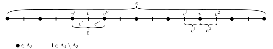
Figure 2: Illustration of the recursion $l\leadsto l-1$ for $l=4$ in the cases $\bar{e}=e_{3,3}$, $e^{\prime}=e_{5,4}$, $e^{\prime\prime}=e_{6,4}$, $v^{\prime}=v_{e,\frac{2}{8}}$, $v=v_{e,\frac{5}{16}}$, $v^{\prime\prime}=v_{e,\frac{3}{8}}$, $e^{1}=e_{12,4}$, $e^{2}=e_{13,4}$, $v^{1}=v_{e,\frac{11}{16}}$, $\bar{v}=v_{e,\frac{6}{8}}$, and $v^{2}=v_{e,\frac{13}{16}}$.

This lemma is an important ingredient in the proof of the induction step for the moments of $W_{e}^{(l)}$.

Proof of Lemma 1.7. Take $\bar{e}\in E_{l-1}$. Let $v$ be the midpoint of $\bar{e}$. It splits it into two edges, which we may call $e^{\prime},e^{\prime\prime}\in E_{l}$; cf. item 2 in Lemma 3.3. Using the recursion equation (3.6), one has

$${\mathbb{E}}[(W^{(l-1)}_{\bar{e}})^{\alpha}]= {\mathbb{E}}\left[\left(\frac{W_{e^{\prime}}^{(l)}W_{e^{\prime\prime}}^{(l)}}{2\beta_{v}^{(l)\neq}}\right)^{\alpha}\right]={\mathbb{E}}[(W_{e^{\prime}}^{(l)}W_{e^{\prime\prime}}^{(l)})^{\alpha}{\mathbb{E}}[(2\beta_{v}^{(l)\neq})^{-\alpha}|W^{(l)}]],$$ (3.10)

$${\mathbb{E}}[\log W^{(l-1)}_{\bar{e}}]= {\mathbb{E}}[\log W_{e^{\prime}}^{(l)}+\log W_{e^{\prime\prime}}^{(l)}+{\mathbb{E}}[\log((2\beta_{v}^{(l)\neq})^{-1})|W^{(l)}]].$$ (3.11)

By item 4 in Lemma 3.3, given $W^{(l)}$, the random variable $(2\beta_{v}^{(l)\neq})^{-1}$ has an inverse Gaussian distribution $\operatorname{IG}((W^{(l)}_{e^{\prime}}+W^{(l)}_{e^{\prime\prime}})^{-1},1)$, hence its conditional expectation equals the first parameter $(W^{(l)}_{e^{\prime}}+W^{(l)}_{e^{\prime\prime}})^{-1}$. In combination with Lemma A.2 and (A.11) in the appendix, we obtain

$${\mathbb{E}}[(2\beta_{v}^{(l)\neq})^{-\alpha}|W^{(l)}]\leq(W^{(l)}_{e^{\prime}}+W^{(l)}_{e^{\prime\prime}})^{-\alpha}\quad\text{for }\alpha\in[0,1],$$ (3.12)

$${\mathbb{E}}[(2\beta_{v}^{(l)\neq})^{-\alpha}|W^{(l)}]\leq C_{\alpha}\quad\text{for }\alpha\in[0,\tfrac{1}{2}),$$ (3.13)

$${\mathbb{E}}[\log((2\beta_{v}^{(l)\neq})^{-1})|W^{(l)}]\leq\min\{-\log(W^{(l)}_{e^{\prime}}+W^{(l)}_{e^{\prime\prime}}),{c_{2}}\}.$$ (3.14)

The next step uses the inequality between arithmetic and geometric mean of two numbers $x,y>0$ in the following form

$$\frac{xy}{x+y}=\frac{1}{2}\frac{\sqrt{xy}}{\frac{1}{2}(x+y)}\sqrt{xy}\leq\frac{1}{2}\sqrt{xy}.$$ (3.15)

Next, we insert these inequalities in (3.10) and (3.11). Using Cauchy Schwarz in (3.16) and independence and identical distribution of $W_{e^{\prime}}^{(l)}$ and $W_{e^{\prime\prime}}^{(l)}$ in (3.17), we conclude

$${\mathbb{E}}[(W^{(l-1)}_{\bar{e}})^{\alpha}]\leq {\mathbb{E}}\left[\left(\frac{W_{e^{\prime}}^{(l)}W_{e^{\prime\prime}}^{(l)}}{W^{(l)}_{e^{\prime}}+W^{(l)}_{e^{\prime\prime}}}\right)^{\alpha}\right]\leq{\mathbb{E}}\left[\left(\frac{1}{2}\sqrt{W_{e^{\prime}}^{(l)}W_{e^{\prime\prime}}^{(l)}}\right)^{\alpha}\right]$$

$$\leq 2^{-\alpha}{\mathbb{E}}[(W_{e^{\prime}}^{(l)})^{\alpha}]^{\frac{1}{2}}{\mathbb{E}}[(W_{e^{\prime\prime}}^{(l)})^{\alpha}]^{\frac{1}{2}}=2^{-\alpha}{\mathbb{E}}[(W_{e^{\prime}}^{(l)})^{\alpha}]\quad\text{for }\alpha\in[0,1],$$ (3.16)

$${\mathbb{E}}[(W^{(l-1)}_{\bar{e}})^{\alpha}]\leq C_{\alpha}{\mathbb{E}}[(W_{e^{\prime}}^{(l)}W_{e^{\prime\prime}}^{(l)})^{\alpha}]$$

$$\leq C_{\alpha}{\mathbb{E}}[(W_{e^{\prime}}^{(l)})^{\alpha}]{\mathbb{E}}[(W_{e^{\prime\prime}}^{(l)})^{\alpha}]=C_{\alpha}{\mathbb{E}}[(W_{e^{\prime}}^{(l)})^{\alpha}]^{2}\quad\text{for }\alpha\in[0,\tfrac{1}{2}),$$ (3.17)

$${\mathbb{E}}[\log W^{(l-1)}_{\bar{e}}]\leq {\mathbb{E}}\left[\log\frac{W_{e^{\prime}}^{(l)}W_{e^{\prime\prime}}^{(l)}}{W^{(l)}_{e^{\prime}}+W^{(l)}_{e^{\prime\prime}}}\right]\leq\frac{1}{2}({\mathbb{E}}[\log W_{e^{\prime}}^{(l)}]+{\mathbb{E}}[\log W_{e^{\prime\prime}}^{(l)}])-\log 2$$

$$= {\mathbb{E}}[\log W_{e^{\prime}}^{(l)}]-\log 2,$$ (3.18)

$${\mathbb{E}}[\log W^{(l-1)}_{\bar{e}}]\leq {\mathbb{E}}[\log W_{e^{\prime}}^{(l)}]+{\mathbb{E}}[\log W_{e^{\prime\prime}}^{(l)}]+{c_{2}}=2{\mathbb{E}}[\log W_{e^{\prime}}^{(l)}]+{c_{2}}.$$ (3.19)

 

One could alternatively obtain ${\mathbb{E}}[\log W^{(l-1)}_{\bar{e}}]\leq{\mathbb{E}}[\log W^{(l)}_{e^{\prime}}]-\log 2$ from (1.12) using $\lim_{\alpha\downarrow 0}(x^{\alpha}-1)/\alpha=\log x$ and interchanging the limit $\alpha\downarrow 0$ with the expectation.

The following proof is based on iteration of the bounds in Lemma 1.7.

Proof of Theorem 1.6. Iterating (1.12) $r-l$ times, we obtain (1.9). For $\alpha\in[0,\frac{1}{2})$, the idea of the proof is to iterate (1.12), starting with $l=r$, as long as it gives a better bound than (1.13), and then switching over to the other bound (1.13). Let $m\in\{l,\ldots,r\}$. Iterating (1.13) $m-l$ times yields

$$C_{\alpha}{\mathbb{E}}[(W^{(l)}_{\bar{e}})^{\alpha}] \leq(C_{\alpha}{\mathbb{E}}[(W^{(m)}_{\tilde{e}})^{\alpha}])^{2^{m-l}}$$ (3.20)

for $\tilde{e}\in E_{m}$. Applying (1.9) with $l$ replaced by $m$, i.e., ${\mathbb{E}}[(W^{(m)}_{\tilde{e}})^{\alpha}]\leq(2^{-\alpha})^{r-m}{\mathbb{E}}[(W^{(r)}_{e^{\prime}})^{\alpha}]$ gives

$$C_{\alpha}{\mathbb{E}}[(W^{(l)}_{\bar{e}})^{\alpha}]\leq\left(C_{\alpha}(2^{-\alpha})^{r-m}{\mathbb{E}}[(W^{(r)}_{e^{\prime}})^{\alpha}]\right)^{2^{m-l}}$$ (3.21)

and (1.10) follows using $W^{(r)}_{e^{\prime}}=W_{e^{\prime}}$. To identify a minimizer, let $X_{m}:=C_{\alpha}(2^{-\alpha})^{r-m}{\mathbb{E}}[W_{e^{\prime}}^{\alpha}]$. Note that the argument of the minimum in (1.10) is given by $X_{m}^{2^{m-l}}$. We observe the following equivalences

$$X_{m}^{2^{m-l}}<X_{m-1}^{2^{m-1-l}}\;\Leftrightarrow\;(X_{m}^{2})^{2^{m-1-l}}<(2^{-\alpha}X_{m})^{2^{m-1-l}}\;\Leftrightarrow\;X_{m}<2^{-\alpha}\;\Leftrightarrow$$

$$m<r-1-\alpha^{-1}\log_{2}(C_{\alpha}{\mathbb{E}}[W_{e^{\prime}}^{\alpha}])\;\Leftrightarrow\;m\leq r-2-\lfloor\alpha^{-1}\log_{2}(C_{\alpha}{\mathbb{E}}[W_{e^{\prime}}^{\alpha}])\rfloor$$ (3.22)

The claim about the minimizer $m_{0}$ in (1.10) follows.

Let $0\leq l\leq m\leq r$. Iterating $r-m$ times the inequality ${\mathbb{E}}[\log W^{(l-1)}_{\bar{e}}]\leq{\mathbb{E}}[\log W^{(l)}_{e^{\prime}}]-\log 2$ from (1.14) yields

$${\mathbb{E}}[\log W^{(m)}_{\tilde{e}}] \leq{\mathbb{E}}[\log W^{(r)}_{e^{\prime}}]-(r-m)\log 2.$$ (3.23)

Iterating $m-l$ times the estimate ${\mathbb{E}}[\log W^{(l^{\prime}-1)}_{\bar{e}}]+{c_{2}}\leq 2({\mathbb{E}}[\log W^{(l^{\prime})}_{e^{\prime}}]+{c_{2}})$ from (1.14), we obtain

$${\mathbb{E}}[\log W^{(l)}_{\bar{e}}]+{c_{2}} \leq 2^{m-l}({\mathbb{E}}[\log W^{(m)}_{\tilde{e}}]+{c_{2}}).$$ (3.24)

Inserting (3.23), the claim (1.11) follows. To identify a minimizer, set $Y_{m}:={\mathbb{E}}[\log W_{e^{\prime}}]-(r-m)\log 2+{c_{2}}=Y_{m-1}+\log 2$. Then, the argument of the minimum in (1.11) equals $2^{m-l}Y_{m}$. The following are equivalent.

$$2^{m-l}Y_{m}<2^{m-1-l}Y_{m-1}\;\Leftrightarrow\;Y_{m}<-\log 2\;\Leftrightarrow\;$$ (3.25)

$$m<r-1-(\log 2)^{-1}({\mathbb{E}}[\log W^{(r)}_{e^{\prime}}]+{c_{2}})\;\Leftrightarrow\;m\leq r-2-\lfloor(\log 2)^{-1}({\mathbb{E}}[\log W^{(r)}_{e^{\prime}}]+{c_{2}})\rfloor$$

The claim for the minimizer $m_{1}$ in (1.11) follows.   

3.2 Application to vrjp and errw

In this section, we apply the recursive construction of effective random weights from the last section to restrictions of vrjp and errw on subdivided graphs. In the following, we use the terms “discrete-time process associated with vrjp” and its abbreviation “discrete vrjp” as synonyms.

Since errw is a mixture of discrete vrjps with Gamma distributed i.i.d. weights, it makes sense not to start only with deterministic weights but more generally with i.i.d. weights, deterministic weights being a special case.

The next proof deals with an approximation of a possibly infinite graph by an increasing sequence of finite subgraphs.

Proof of Theorem 1.4. Consider an increasing sequence $\Lambda^{N}\uparrow\Lambda$, $N\in{\mathbb{N}}_{0}$, of finite connected vertex sets in $G$ with $\rho\in\Lambda_{0}$. Let $G^{N}$ be the subgraph of $G$ with vertex set $\Lambda^{N}$ and edge set $E^{N}=\{e\in E:\;e\subseteq\Lambda^{N}\}$, and $G^{N}_{r}=(\Lambda^{N}_{r},E^{N}_{r})$ be the corresponding subdivided graph, where every edge in $E^{N}$ has been replaced by a series of $2^{r}$ edges. Consider the discrete vrjp $X^{N}$ on $G^{N}_{r}$ with random weights $W_{e}$, $e\in E^{N}_{r}$. By Theorem 1.2, its restriction $(X^{N})^{\Lambda_{l}^{N}\neq}$ to $G^{N}_{l}$ is a mixture of discrete vrjps with random weights $W_{\bar{e}}^{(l)}$, $\bar{e}\in E_{l}^{N}$, fulfilling the properties in Lemma 3.3. We emphasize that the finite-dimensional marginals $(W_{\bar{e}}^{(l)})_{\bar{e}\in F}$, $F\subseteq E_{l}$ finite, do not depend on the size $N$ of the graph, whenever $N$ is large enough so that $F\subseteq E_{l}^{N}$. This allows us to take the same random variables $W_{\bar{e}}^{(l)}$ for all $N$. Moreover, by part 5 of Lemma 3.3, the family of weights $(W_{e}^{(l)})_{e\in E_{l}}$ is independent or i.i.d., respectively, if $(W_{e})_{e\in E}$ has this property.

Given $m\in{\mathbb{N}}$, consider only the first $m$ steps of the restrictions $X^{\Lambda_{l}\neq}$ and $(X^{N})^{\Lambda_{l}^{N}\neq}$. If $N$ is large enough, these two restrictions have the same law because they have no chance to enter $\Lambda_{l}\setminus\Lambda_{l}^{N}$. It follows that $X^{\Lambda_{l}\neq}$ is a mixture of discrete vrjp with random weights $W_{\bar{e}}^{(l)}$, $\bar{e}\in E_{l}$ because this is true for its restriction to any given number $m$ of steps. Using the estimate (1.9) from Theorem 1.6 and the assumption on ${\mathbb{E}}[W_{e}^{\alpha}]$ for some $\alpha\in(0,\frac{1}{4}]$, we obtain for all $\bar{e}\in E_{l}$ and $e\in E_{r}$,

$${\mathbb{E}}[(W^{(l)}_{\bar{e}})^{\alpha}] \leq(2^{-\alpha})^{r-l}{\mathbb{E}}[(W_{e})^{\alpha}]\leq{c_{1}}.$$ (3.26)

The claim follows from Fact 1.3.   

Finally, the result for errw is obtained by specializing the i.i.d. weights to i.i.d. Gamma distributed weights as follows.

Proof of Theorem 1.5. By [ST15, Theorem 1], the edge-reinforced random walk on $G_{r}$ is a mixture of the discrete vrjp with i.i.d. Gamma($a$,1)-distributed weights $W_{e}$, $e\in E_{r}$. We observe that for all $\alpha\geq 0$ one has ${\mathbb{E}}[W_{e}^{\alpha}]=\Gamma(a+\alpha)/\Gamma(a)$. Consequently, the claim follows from Theorem 1.4.   

4 Proofs for the non-linear hyperbolic sigma model

Recall the setup of Section 1.3. Set $H^{3|2}_{+}:=\{\sigma=(x,y,z,\xi,\eta)\in\mathcal{A}_{0}^{3}\times\mathcal{A}_{1}^{2}:\left\langle{\sigma,\sigma}\right\rangle<0,\operatorname{body}z>0\}$. For $\sigma\in H^{3|2}_{+}$, let $\|\sigma\|:=\sqrt{-\left\langle{\sigma,\sigma}\right\rangle}$. The following lemma describes the super-Laplace transform of the canonical superintegration form $\mathcal{D}\sigma$ on $H^{2|2}$. Recall from Section 1.3 that the graph $(\Lambda,E_{+})$ with edge set $E_{+}=\{\{i,j\}\subseteq\Lambda:W_{ij}>0\}$ is connected, which implies that at least one $W_{1i}$ is strictly positive for every vertex $1\in\Lambda$.

Lemma 4.1 (Integration of one variable)

Let $1\in\Lambda$ and set $1^{c}=\Lambda\setminus\{1\}$. One has

$$\int_{H^{2|2}}\mathcal{D}\sigma_{1}\,e^{\sum_{i\in 1^{c}}W_{1i}\left\langle{\sigma_{1},\sigma_{i}}\right\rangle}=e^{-\|\sum_{i\in 1^{c}}W_{1i}\sigma_{i}\|},$$ (4.1)

and consequently,

$$\int_{H^{2|2}}\mathcal{D}\sigma_{1}\,e^{\frac{1}{2}\sum_{i,j\in\Lambda}W_{ij}(1+\left\langle{\sigma_{i},\sigma_{j}}\right\rangle)}= e^{\frac{1}{2}\sum_{i,j\in 1^{c}}W_{ij}(1+\left\langle{\sigma_{i},\sigma_{j}}\right\rangle)+\sum_{i\in 1^{c}}W_{1i}-\|\sum_{i\in 1^{c}}W_{1i}\sigma_{i}\|}.$$ (4.2)

Proof. By the convexity of $H^{3|2}_{+}$, one has $\sum_{i\in 1^{c}}W_{1i}\sigma_{i}\in H^{3|2}_{+}$ and hence [DMR22, Lemma 3.2, second equality in (3.1)] is applicable and yields

$$\int_{H^{2|2}}\mathcal{D}\sigma_{1}\,e^{\sum_{i\in 1^{c}}W_{1i}\left\langle{\sigma_{1},\sigma_{i}}\right\rangle}= \int_{H^{2|2}}\mathcal{D}\sigma_{1}\,e^{\left\langle{\sigma_{1},\sum_{i\in 1^{c}}W_{1i}\sigma_{i}}\right\rangle}=e^{-\|\sum_{i\in 1^{c}}W_{1i}\sigma_{i}\|}.$$ (4.3)

The second claim (4.2) follows from (4.1) using $\left\langle{\sigma_{1},\sigma_{1}}\right\rangle=-1$ and decomposing the exponent as follows

$$\frac{1}{2}\sum_{i,j\in\Lambda}W_{ij}(1+\left\langle{\sigma_{i},\sigma_{j}}\right\rangle)=\frac{1}{2}\sum_{i,j\in 1^{c}}W_{ij}(1+\left\langle{\sigma_{i},\sigma_{j}}\right\rangle)+\sum_{i\in 1^{c}}W_{1i}+\sum_{i\in 1^{c}}W_{1i}\left\langle{\sigma_{1},\sigma_{i}}\right\rangle.$$ (4.4)

 

This lemma is the key ingredient for analyzing the restriction of the $H^{2|2}$ model.

Proof of Theorem 1.8. The second equation in (1.19) follows from the restriction property of the betas; see Remark 2.3. The proof of the first equation in (1.19) is by induction with respect to the cardinality of $I$. For $I=\emptyset$, there is nothing to prove. As induction hypothesis, assume that formula (1.19) holds for given $I\subsetneq\Lambda\setminus\{\rho\}$ and $J=\Lambda\setminus I$. For the induction step, take $i\in J$, $i\neq\rho$, and set $\tilde{I}=I\cup\{i\}$, $\tilde{J}=\Lambda\setminus\tilde{I}=J\setminus\{i\}$. For any superfunction $f$ on $(H^{2|2})^{\tilde{J}}$ being compactly supported or at least sufficiently fast decaying so that the integral on the left-hand side of (4.5) is well-defined, the induction hypothesis yields

$$\int_{(H^{2|2})^{\Lambda}}\mu_{\Lambda}^{W}(\sigma_{\Lambda})f(\sigma_{\tilde{J}})=\int_{{\mathbb{R}}^{\Lambda}}\nu_{\Lambda}^{W}(d\beta)\int_{(H^{2|2})^{J}}\mu_{J}^{W^{J}(\beta_{I})}(\sigma_{J})f(\sigma_{\tilde{J}}).$$ (4.5)

We fix $\beta\in{\mathbb{R}}^{\Lambda}$, abbreviate $W^{J}=W^{J}(\beta_{I})$ when there is no risk of confusion, and set $g(\sigma_{\tilde{J}})=e^{\frac{1}{2}\sum_{j,k\in\tilde{J}}W^{J}_{jk}(1+\left\langle{\sigma_{j},\sigma_{k}}\right\rangle)}f(\sigma_{\tilde{J}})$. We split the integrand into a part which does not involve $\sigma_{i}$ and the remaining part involving $\left\langle{\sigma_{i},\sigma_{j}}\right\rangle$, $j\in\tilde{J}$:

$$\int_{(H^{2|2})^{J}}\mu_{J}^{W^{J}(\beta_{I})}(\sigma_{J})f(\sigma_{\tilde{J}})=\int_{(H^{2|2})^{J}}\mathcal{D}\sigma_{J}\,e^{\frac{1}{2}\sum_{j,k\in J}W^{J}_{ij}(1+\left\langle{\sigma_{j},\sigma_{k}}\right\rangle)}f(\sigma_{\tilde{J}})$$

$$=\int_{(H^{2|2})^{\tilde{J}}}\mathcal{D}\sigma_{\tilde{J}}\,g(\sigma_{\tilde{J}})\int_{H^{2|2}}\mathcal{D}\sigma_{i}e^{\sum_{j\in\tilde{J}}W^{J}_{ij}(1+\left\langle{\sigma_{i},\sigma_{j}}\right\rangle)}.$$ (4.6)

Note that the term $W^{J}_{ii}(1+\left\langle{\sigma_{i},\sigma_{i}}\right\rangle)=0$ has been dropped. By formula (4.1) in Lemma 4.1 and using the abbreviation $W^{J}_{i}:=\sum_{j\in\tilde{J}}W^{J}_{ij}=\sum_{j\in J\setminus\{i\}}W^{J}_{ij}$, the single-spin integral in the last expression equals

$$\int_{H^{2|2}}\mathcal{D}\sigma_{i}e^{\sum_{j\in\tilde{J}}W^{J}_{ij}(1+\left\langle{\sigma_{i},\sigma_{j}}\right\rangle)}=e^{W^{J}_{i}-\left\|\sum_{j\in\tilde{J}}W^{J}_{ij}\sigma_{j}\right\|}=e^{W^{J}_{i}(1-\|\sum_{j\in\tilde{J}}\frac{W^{J}_{ij}}{W^{J}_{i}}\sigma_{j}\|)}.$$ (4.7)

Using auxiliary random variables $X\sim\operatorname{IG}\left(\frac{W^{J}_{i}}{2},\frac{(W^{J}_{i})^{2}}{2}\right)$ and $Y=\frac{2X}{(W^{J}_{i})^{2}}\sim\operatorname{IG}\left((W^{J}_{i})^{-1},1\right)$ with inverse Gaussian distributions, cf. Appendix A, on some auxiliary probability space with expectation operator denoted by $E$, Lemma A.1 allows us to rewrite the last expression in the form

$$\eqref{eq:Integrate-single-spin} =E\left[e^{X(1-\|\sum_{j\in\tilde{J}}\frac{W^{J}_{ij}}{W^{J}_{i}}\sigma_{j}\|^{2})}\right]=E\left[e^{\frac{X}{(W^{J}_{i})^{2}}\left((W^{J}_{i})^{2}+\sum_{j,k\in\tilde{J}}W^{J}_{ij}W^{J}_{ik}\left\langle{\sigma_{j},\sigma_{k}}\right\rangle\right)}\right]$$

$$=E\left[e^{\frac{Y}{2}\sum_{j,k\in\tilde{J}}W^{J}_{ij}W^{J}_{ik}\left(1+\left\langle{\sigma_{j},\sigma_{k}}\right\rangle\right)}\right].$$ (4.8)

Using the notation (1.1), we take the specific choice $({\mathbb{R}}^{J},\mathcal{B}({\mathbb{R}}^{J}),\nu_{J}^{W^{J}}(d\tilde{\beta}))$ and $Y=(2\tilde{\beta_{i}}-W^{J}_{ii})^{-1}=([H_{J,\tilde{\beta}}^{W^{J}}]_{ii})^{-1}$ for the auxiliary probability space and the auxiliary random variable $Y$, respectively. Indeed, $Y\sim\operatorname{IG}((W^{J}_{i})^{-1},1)$ for this choice is a consequence (2.13). Summarizing, this shows

$$\int_{H^{2|2}}\mathcal{D}\sigma_{i}e^{\sum_{j\in\tilde{J}}W^{J}_{ij}(1+\left\langle{\sigma_{i},\sigma_{j}}\right\rangle)}= \int_{{\mathbb{R}}^{J}}\nu_{J}^{W^{J}}(d\tilde{\beta})e^{\frac{1}{2}\sum_{j,k\in\tilde{J}}\frac{W^{J}_{ij}W^{J}_{ik}}{2\tilde{\beta_{i}}-W^{J}_{ii}}\left(1+\left\langle{\sigma_{j},\sigma_{k}}\right\rangle\right)}.$$ (4.9)

We substitute this in (4) to obtain

$$\int_{(H^{2|2})^{\tilde{J}}}\mu_{J}^{W^{J}(\beta_{I})}(\sigma_{J})f(\sigma_{\tilde{J}})=\int_{(H^{2|2})^{\tilde{J}}}\mathcal{D}\sigma_{\tilde{J}}\,g(\sigma_{\tilde{J}})\int_{{\mathbb{R}}^{J}}\nu_{J}^{W^{J}}(d\tilde{\beta})e^{\frac{1}{2}\sum_{j,k\in\tilde{J}}\frac{W^{J}_{ij}W^{J}_{ik}}{2\tilde{\beta_{i}}-W^{J}_{ii}}\left(1+\left\langle{\sigma_{j},\sigma_{k}}\right\rangle\right)}$$

$$=\int_{{\mathbb{R}}^{J}}\nu_{J}^{W^{J}}(d\tilde{\beta})\int_{(H^{2|2})^{\tilde{J}}}\mathcal{D}\sigma_{\tilde{J}}\,f(\sigma_{\tilde{J}})e^{\frac{1}{2}\sum_{j,k\in\tilde{J}}\left[W^{J}_{jk}+\frac{W^{J}_{ji}W^{J}_{ik}}{2\tilde{\beta_{i}}-W^{J}_{ii}}\right]\left(1+\left\langle{\sigma_{j},\sigma_{k}}\right\rangle\right)}$$

$$=\int_{{\mathbb{R}}^{J}}\nu_{J}^{W^{J}}(d\tilde{\beta})\int_{(H^{2|2})^{\tilde{J}}}\mu_{\tilde{J}}^{W^{\tilde{J}}(\beta_{I},\tilde{\beta}_{i})}(\sigma_{\tilde{J}})\,f(\sigma_{\tilde{J}})$$ (4.10)

because

$$\left(W^{J}_{jk}+\frac{W^{J}_{ji}W^{J}_{ik}}{2\tilde{\beta_{i}}-W^{J}_{ii}}\right)_{j,k\in\tilde{J}}= W^{J}_{\tilde{J}\tilde{J}}+W^{J}_{\tilde{J}i}\left[\left(H_{J,\tilde{\beta}}^{W^{J}}\right)_{ii}\right]^{-1}W^{J}_{i\tilde{J}}$$

$$= (W^{J})^{\tilde{J}}(\tilde{\beta}_{i})=W^{\tilde{J}}(\beta_{I},\tilde{\beta}_{i}),$$ (4.11)

where we used $W^{J}=W^{J}(\beta_{I})$ and (3.2) with $J\setminus\tilde{J}=\{i\}$. Taking now $\beta$ random, we insert the result in (4.5) and obtain

$$\int_{(H^{2|2})^{\Lambda}}\mu_{\Lambda}^{W}(\sigma_{\Lambda})f(\sigma_{\tilde{J}})=\int_{{\mathbb{R}}^{\Lambda}}\nu_{\Lambda}^{W}(d\beta)\int_{{\mathbb{R}}^{J}}\nu_{J}^{W^{J}(\beta_{I})}(d\tilde{\beta})\int_{(H^{2|2})^{\tilde{J}}}\mu_{\tilde{J}}^{W^{\tilde{J}}(\beta_{I},\tilde{\beta}_{i})}(\sigma_{\tilde{J}})\,f(\sigma_{\tilde{J}}).$$ (4.12)

By the conditioning property cited in Remark 2.3, the conditional law of $\beta_{J}$ given $\beta_{I}$ with respect to $\nu_{\Lambda}^{W}$ equals $\nu_{J}^{W^{J}(\beta_{I})}$. In other words, for any integrable function $h(\beta_{I},\beta_{J})$, one has

$$\int_{{\mathbb{R}}^{\Lambda}}\nu_{\Lambda}^{W}(d\beta)\int_{{\mathbb{R}}^{J}}\nu_{J}^{W^{J}(\beta_{I})}(d\tilde{\beta})\,h(\beta_{I},\tilde{\beta})=\int_{{\mathbb{R}}^{\Lambda}}\nu_{\Lambda}^{W}(d\beta)\,h(\beta_{I},\beta_{J}).$$ (4.13)

Recall $i\in J$. Applying the last identity with

$$h(\beta_{I},\beta_{J})=\int_{(H^{2|2})^{\tilde{J}}}\mu_{\tilde{J}}^{W^{\tilde{J}}(\beta_{I},(\beta_{J})_{i})}(\sigma_{\tilde{J}})\,f(\sigma_{\tilde{J}}),$$ (4.14)

and observing $(\beta_{I},(\beta_{J})_{i})=\beta_{\tilde{I}}$, we conclude the induction step with the calculation

$$\int_{(H^{2|2})^{\Lambda}}\mu_{\Lambda}^{W}(\sigma_{\Lambda})f(\sigma_{\tilde{J}})=\int_{{\mathbb{R}}^{\Lambda}}\nu_{\Lambda}^{W}(d\beta)\int_{(H^{2|2})^{\tilde{J}}}\mu_{\tilde{J}}^{W^{\tilde{J}}(\beta_{\tilde{I}})}(\sigma_{\tilde{J}})f(\sigma_{\tilde{J}}).$$ (4.15)

 

Appendix A Facts about inverse Gaussians

The density of an inverse Gaussian distribution $\operatorname{IG}(\mu,\lambda)$ with parameters $\mu,\lambda>0$ is given by

$$f(x)=\sqrt{\frac{\lambda}{2\pi x^{3}}}\exp\left(-\frac{\lambda(x-\mu)^{2}}{2\mu^{2}x}\right),\quad x>0.$$ (A.1)

For $X\sim\operatorname{IG}(\mu,\lambda)$, one has $E[X]=\mu$ and the Laplace transform is given by

$$\phi(t)=E[e^{tX}]=e^{\frac{\lambda}{\mu}\left(1-\sqrt{1-\frac{2\mu^{2}t}{\lambda}}\right)},\quad t\leq\frac{\lambda}{2\mu^{2}}.$$ (A.2)

The following special case of the Laplace transform is used in the proof of Theorem 1.8.

Lemma A.1 (Laplace transform)

If $X\sim\operatorname{IG}(\frac{a}{2},\frac{a^{2}}{2})$ for some $a>0$, then

$$E[e^{(1-s)X}]=e^{a(1-\sqrt{s})},\quad s\geq 0.$$ (A.3)

Proof. Setting $\mu=\frac{a}{2}$ and $\lambda=\frac{a^{2}}{2}$, this follows from (A.2) using $\frac{\lambda}{\mu}=a$ and $\frac{2\mu^{2}}{\lambda}=1$.   

Our estimates for the effective weights in Theorem 1.6 require the estimates in the following Lemmas A.2 and A.3.

Lemma A.2 (Estimates for some moments)

For $W>0$ and $X_{W}\sim\operatorname{IG}(W^{-1},1)$, with the constant $C_{\alpha}$ from Theorem 1.6, one has

$$E[X_{W}^{\alpha}]\leq W^{-\alpha}\hskip 65.44142pt\text{ for }\alpha\in[0,1],$$ (A.4)

$$E[X_{W}^{\alpha}]\leq C_{\alpha}\quad\text{ for }\alpha\in[0,\tfrac{1}{2}),\qquad\lim_{W\downarrow 0}E[X_{W}^{\alpha}]=C_{\alpha}.$$ (A.5)

Proof. Using Jensen’s inequality for the concave function $x^{\alpha}$, we obtain $E[X_{W}^{\alpha}]\leq E[X_{W}]^{\alpha}=W^{-\alpha}$ for $0\leq\alpha\leq 1$.

We prove now the second bound. By (A.1), one has

$$f_{\alpha}(W):=E[X_{W}^{\alpha}]=\frac{1}{\sqrt{2\pi}}\int_{0}^{\infty}x^{\alpha-\frac{3}{2}}e^{-\frac{(Wx-1)^{2}}{2x}}\,dx$$ (A.6)

for all $\alpha\in[0,\frac{1}{2})$. Taking the derivative with respect to $W$ and substituting first $y=Wx$ and then $z=1/y$ it follows

$$f_{\alpha}^{\prime}(W)= \frac{1}{\sqrt{2\pi}}\int_{0}^{\infty}x^{\alpha-\frac{3}{2}}(1-Wx)e^{-\frac{W}{2}(Wx+(Wx)^{-1}-2)}\,dx$$

$$= \frac{W^{\frac{1}{2}-\alpha}}{\sqrt{2\pi}}\int_{0}^{\infty}y^{\alpha-\frac{3}{2}}(1-y)e^{-\frac{W}{2}(y+y^{-1}-2)}\,dy$$

$$= -\frac{W^{\frac{1}{2}-\alpha}}{\sqrt{2\pi}}\int_{0}^{\infty}z^{-\alpha-\frac{3}{2}}(1-z)e^{-\frac{W}{2}(z+z^{-1}-2)}\,dz.$$ (A.7)

Taking the average of the last two expressions and using $(y^{\alpha}-y^{-\alpha})(1-y)\leq 0$ for $y\geq 0$ and $\alpha>0$ yields

$$f_{\alpha}^{\prime}(W)= \frac{W^{\frac{1}{2}-\alpha}}{2\sqrt{2\pi}}\int_{0}^{\infty}y^{-\frac{3}{2}}(y^{\alpha}-y^{-\alpha})(1-y)e^{-\frac{W}{2}(y+y^{-1}-2)}\,dy\leq 0.$$ (A.8)

Hence, the function $f_{\alpha}$ is decreasing, which implies $f_{\alpha}(W)\leq\lim_{w\downarrow 0}f_{\alpha}(w)$ for all $W>0$. For $0\leq\alpha<\frac{1}{2}$, we evaluate this limit as follows. Using dominated convergence with the integrable upper bound $x^{\alpha-\frac{3}{2}}e^{1-\frac{1}{2x}}$ for the integrand in (A.6) with $0<W\leq 1$ and then substituting $y=(2x)^{-1}$ , we conclude

$$f_{\alpha}(W)\leq\lim_{w\downarrow 0}f_{\alpha}(w)=\frac{1}{\sqrt{2\pi}}\int_{0}^{\infty}x^{\alpha-\frac{3}{2}}e^{-\frac{1}{2x}}\,dx=\frac{1}{2^{\alpha}\sqrt{\pi}}\int_{0}^{\infty}y^{-\alpha-\frac{1}{2}}e^{-y}\,dy=C_{\alpha}.$$ (A.9)

 

Lemma A.3 (Estimate for the logarithmic moment)

For $W>0$ and $X_{W}\sim\operatorname{IG}(W^{-1},1)$, one has

$$E[\log X_{W}]= -\log W-\int_{0}^{\infty}\frac{e^{-u}}{u+2W}\,du=e^{2W}\int_{0}^{2W}(\log t+\gamma)e^{-t}\,dt+{c_{2}}$$ (A.10)

with ${c_{2}}$ and $\gamma$ specified in Theorem 1.6. Furthermore, the following bounds hold

$$-\log(W+\tfrac{1}{2})\leq E[\log X_{W}] \leq\min\{-\log W,{c_{2}}\}\quad\text{for }W>0,$$ (A.11)

$${c_{2}}+4W(\log W+{c_{2}}-1)\leq E[\log X_{W}] \leq{c_{2}}\quad\text{for }0<W\leq\tfrac{1}{2}e^{-\gamma},$$ (A.12)

$$\lim_{W\to 0}E[\log X_{W}] ={c_{2}}.$$ (A.13)

Proof. By (A.1), the density of $X_{W}$ is given by

$$f(x)=\sqrt{\frac{1}{2\pi x^{3}}}e^{-\frac{(Wx-1)^{2}}{2x}},$$ (A.14)

$x>0$. Hence, $\log X_{W}$ has the density

$$g(u)=f(e^{u})e^{u}=\frac{1}{\sqrt{2\pi}}e^{-\frac{1}{2}(We^{u}-1)^{2}e^{-u}}e^{-\frac{u}{2}},$$ (A.15)

$u\in{\mathbb{R}}$, with respect to the Lebesgue measure on ${\mathbb{R}}$. Rewriting the exponent of the first exponential as

$$\frac{1}{2}(We^{u}-1)^{2}e^{-u}=\frac{1}{2}W(We^{u}+(We^{u})^{-1}-2)=W[\cosh(u+\log W)-1]$$ (A.16)

yields the density

$$g(u)=\frac{1}{\sqrt{2\pi}}e^{-W[\cosh(u+\log W)-1]-\frac{u}{2}},\quad u\in{\mathbb{R}}.$$ (A.17)

Using the substitution $v=u+\log W$, we obtain

$$E[\log X_{W}]= \frac{1}{\sqrt{2\pi}}\int_{\mathbb{R}}ue^{-W[\cosh(u+\log W)-1]-\frac{u}{2}}\,du$$

$$= -\log W+\sqrt{\frac{W}{2\pi}}e^{W}\int_{\mathbb{R}}ve^{-W\cosh v-\frac{v}{2}}\,dv.$$ (A.18)

Recall the modified Bessel function of second kind $K_{p}$, $p\in{\mathbb{R}}$. By [AS64, 9.6.24], for $w>0$, one has

$$K_{p}(w)=\int_{0}^{\infty}e^{-w\cosh v}\cosh(pv)\,dv=\frac{1}{2}\int_{\mathbb{R}}e^{-w\cosh v}e^{pv}\,dv.$$ (A.19)

Taking the derivative with respect to $p$ yields

$$\partial_{p}K_{p}(w)=\frac{1}{2}\int_{\mathbb{R}}ve^{-w\cosh v}e^{pv}\,dv.$$ (A.20)

Combining this with (A.18), we obtain

$$E[\log X_{W}]= -\log W+\sqrt{\frac{2W}{\pi}}e^{W}\partial_{p}K_{p}(W)|_{p=-\frac{1}{2}}.$$ (A.21)

By [Rya21, Page 1],

$$\partial_{p}K_{p}(w)|_{p=\frac{1}{2}}= K_{\frac{1}{2}}(w)\int_{0}^{\infty}\frac{e^{-u}}{u+2w}\,du.$$ (A.22)

Combining this with $K_{p}(w)=K_{-p}(w)$, cf. [AS64, 9.6.6], and $K_{\frac{1}{2}}(w)=\sqrt{\pi/(2w)}e^{-w}$, cf. [AS64, 10.2.17], yields

$$\partial_{p}K_{p}(w)|_{p=-\frac{1}{2}}(w)=-\partial_{p}K_{p}(w)|_{p=\frac{1}{2}}(w)= -\sqrt{\frac{\pi}{2w}}e^{-w}\int_{0}^{\infty}\frac{e^{-u}}{u+2w}\,du.$$ (A.23)

This proves the first equality in the claim (A.10). In particular, $E[\log X_{W}]\leq-\log W$.

To prove the second equality in (A.10), we observe that

$$\int_{0}^{\infty}(\log t+\gamma)e^{-t}\,dt=0$$ (A.24)

by the expression (1.8) for the Euler Mascheroni constant; note that the integrand is integrable both at $t=0$ and $t=\infty$. Thus, using integration by parts, we conclude

$$e^{2W}\int_{0}^{2W}(\log t+\gamma)e^{-t}\,dt=-e^{2W}\int_{2W}^{\infty}(\log t+\gamma)e^{-t}\,dt$$

$$= -(\log(2W)+\gamma)-\int_{2W}^{\infty}\frac{e^{2W-t}}{t}\,dt=-\log W-\log 2-\gamma-\int_{0}^{\infty}\frac{e^{-u}}{u+2W}\,du.$$ (A.25)

Next, we show $f(W):=\int_{0}^{2W}(\log t+\gamma)e^{-t}\,dt\leq 0$. Note that the integrand $(\log t+\gamma)e^{-t}$ is negative for $0<t<e^{-\gamma}$ and positive for $t>e^{-\gamma}$. Hence, the function $f$ is decreasing on the interval $[0,e^{-\gamma}]$ and increasing on $[e^{-\gamma},\infty]$. Since $f(0)=0=f(\infty)$ by (A.24), the claim $f\leq 0$ and hence $E[\log X_{W}]\leq{c_{2}}$ follow. We conclude that the upper bound in (A.11) is valid.

We proceed with the lower bound in (A.11). We have

$$\int_{0}^{\infty}\frac{e^{-u}}{u+2W}\,du=e^{2W}E_{1}(2W)\leq\log\left(1+\frac{1}{2W}\right)$$ (A.26)

with the exponential integral $E_{1}(x)=\int_{x}^{\infty}\frac{e^{-u}}{u}\,du$ using the known bound $e^{x}E_{1}(x)\leq\log(1+1/x)$ for all $x>0$, cf. [AS64, 5.1.20]. Substituting this in (A.10), we conclude

$$E[\log X_{W}]\geq-\log W-\log\left(1+\frac{1}{2W}\right)=-\log(W+\tfrac{1}{2}).$$ (A.27)

Assume now $0<W\leq\frac{1}{2}e^{-\gamma}$. The upper bound in (A.12) is already contained in (A.11); it remains to show the lower bound. We estimate the last integral in (A.10), using that $e^{2W}\leq\exp(e^{-\gamma})=1.753\ldots\leq 2$ and $\log t+\gamma\leq 0$ hold for $0<t\leq e^{-\gamma}$, to obtain

$$E[\log X_{W}]-{c_{2}}= e^{2W}\int_{0}^{2W}(\log t+\gamma)e^{-t}\,dt\geq 2\int_{0}^{2W}(\log t+\gamma)\,dt$$

$$= 4W(\log W+{c_{2}}-1).$$ (A.28)

This proves (A.12) and (A.13).   

We remark that the upper bound $E[\log X_{w}]\leq{c_{2}}$ in (A.12) can also be obtained from (A.5) in the form $E[(X_{W}^{\alpha}-1)/\alpha]\leq(C_{\alpha}-1)/\alpha$, taking the limit as $\alpha\downarrow 0$, interchanging limit and expectation, and using $\partial_{\alpha}C_{\alpha}|_{\alpha=0}={c_{2}}$.

Acknowledgements.

This work is funded by the Deutsche Forschungsgemeinschaft (DFG, German Research Foundation) within SPP 2265 Random Geometric Systems (Project number 443757604) and the Hausdorff Center for Mathematics (project ID 390685813). The authors would like to thank the Isaac Newton Institute for Mathematical Sciences, Cambridge, for support and hospitality during the programme Stochastic systems for anomalous diffusion (EPSRC grant no EP/R014604/1.34), where part of this work was undertaken.

References

- [ACK14] O. Angel, N. Crawford, and G. Kozma. Localization for linearly edge reinforced random walks. Duke Math. J., 163(5):889–921, 2014.
- [AS64] M. Abramowitz and I.A. Stegun. Handbook of mathematical functions with formulas, graphs, and mathematical tables, volume No. 55 of National Bureau of Standards Applied Mathematics Series. U. S. Government Printing Office, Washington, DC, 1964.
- [CD86] D. Coppersmith and P. Diaconis. Random walk with reinforcement. Unpublished manuscript, 1986.
- [Dia88] P. Diaconis. Recent progress on de Finetti’s notions of exchangeability. In Bayesian statistics, 3 (Valencia, 1987), pages 111–125. Oxford Univ. Press, New York, 1988.
- [DMR22] M. Disertori, F. Merkl, and S.W.W. Rolles. The non-linear supersymmetric hyperbolic sigma model on a complete graph with hierarchical interactions. ALEA Lat. Am. J. Probab. Math. Stat., 19(2):1629–1648, 2022.
- [DSZ10] M. Disertori, T. Spencer, and M.R. Zirnbauer. Quasi-diffusion in a 3D supersymmetric hyperbolic sigma model. Comm. Math. Phys., 300(2):435–486, 2010.
- [DV02] B. Davis and S. Volkov. Continuous time vertex-reinforced jump processes. Probab. Theory Related Fields, 123(2):281–300, 2002.
- [LW20] G. Letac and J. Wesołowski. Multivariate reciprocal inverse Gaussian distributions from the Sabot-Tarrès-Zeng integral. J. Multivariate Anal., 175:104559, 18, 2020.
- [MR06] F. Merkl and S.W.W. Rolles. Linearly edge-reinforced random walks. In Dynamics and stochastics. Festschrift in honor of M. S. Keane. Selected papers based on the presentations at the conference ‘Dynamical systems, probability theory, and statistical mechanics’, Eindhoven, The Netherlands, January 3–7, 2005, on the occasion of the 65th birthday of Mike S. Keane., pages 66–77. Beachwood, OH: IMS, Institute of Mathematical Statistics, 2006.
- [MR09] F. Merkl and S.W.W. Rolles. Recurrence of edge-reinforced random walk on a two-dimensional graph. Ann. Probab., 37(5):1679–1714, 2009.
- [PA24] R. Poudevigne-Auboiron. Monotonicity and phase transition for the VRJP and the ERRW. J. Eur. Math. Soc. (JEMS), 26(3):789–816, 2024.
- [Rya21] C. Ryavec. BesselK derivatives with respect to order at one half. Preprint, arxiv 2105.00869, 2021.
- [Sab21] C. Sabot. Polynomial localization of the 2D-vertex reinforced jump process. Electron. Commun. Probab., 26:Paper No. 1, 9, 2021.
- [ST15] C. Sabot and P. Tarrès. Edge-reinforced random walk, vertex-reinforced jump process and the supersymmetric hyperbolic sigma model. J. Eur. Math. Soc. (JEMS), 17(9):2353–2378, 2015.
- [STZ17] C. Sabot, P. Tarrès, and X. Zeng. The vertex reinforced jump process and a random Schrödinger operator on finite graphs. Ann. Probab., 45(6A):3967–3986, 2017.
- [Swa20] A. Swan. Superprobability on graphs (PhD thesis). University of Cambridge, https://doi.org/10.17863/CAM.72414, 2020.
- [SZ19] C. Sabot and X. Zeng. A random Schrödinger operator associated with the vertex reinforced jump process on infinite graphs. J. Amer. Math. Soc., 32(2):311–349, 2019.