Sensitivity Analysis of emissions Markets: A Discrete-Time Radner Equilibrium Approach

Abstract.

Emissions markets play a crucial role in reducing pollution by encouraging firms to minimize costs. However, their structure heavily relies on the decisions of policymakers, on the future economic activities, and on the availability of abatement technologies. This study examines how changes in regulatory standards, firms’ abatement costs, and emissions levels affect allowance prices and firms’ efforts to reduce emissions. This is done in a Radner equilibrium framework encompassing inter-temporal decision-making, uncertainty, and a comprehensive assessment of the market dynamics and outcomes. The results of this research have the potential to assist policymakers in enhancing the structure and efficiency of emissions trading systems, through an in-depth comprehension of the reactions of market stakeholders towards different market situations.

Keywords: emissions, carbon market, Radner equilibrium, sensitivity analysis.

2020 Mathematics Subject Classification: 91B76, 91B51, 93E20, 49K40.

1. Introduction

1.1. Motivation, Approach, and Theoretical Contribution

The global effort to combat climate change, as exemplified by the Paris Agreement (United Nations, 2015), has led to regulatory measures aimed at reducing greenhouse gas emissions. Market-based strategies, particularly emissions markets, have become a key approach. In Europe, carbon emissions are regulated through the Emissions Trading System (ETS), which follows a ”cap-and-trade” principle (Woerdman, Roggenkamp, and Holwerda, 2021). This system sets a cap on total emissions for each polluter, allowing them to trade their rights in the market, thereby enhancing cost-effectiveness. It has gained popularity, with over 46 cap-and-trade systems are active worldwide (Blanchard, Gollier, and Tirole, 2023).

Despite their popularity, emission markets are complex systems influenced by various factors, including regulatory policies, market behaviors, and economic conditions. Therefore, it is essential for regulators to have a deeper understanding of these market dynamics to maintain the effectiveness and efficiency of their policies. Polluters must also understand these dynamics to effectively manage the risk of carbon pricing. One effective way to analyze these market dynamics is through sensitivity analysis, which is the main focus of this research. Sensitivity analysis is important for examining how variations in key input factors impact market outcomes, including allowance prices and firms’ abatement efforts. By understanding these relationships, stakeholders can make more informed decisions and improve the overall functioning of emission markets.

To achieve our goal, a discrete-time Radner equilibrium cap-and-trade model is utilized. The Radner equilibrium is well-suited for incomplete markets, as it incorporates uncertainty, limited financial instruments, and firms’ expectations, providing a more realistic analysis of market dynamics and inefficiencies than complete market models. The study examines two main sources of uncertainty in the economy: the emission levels of firms and the emissions cap. Our sensitivity analysis focuses on a two-agent configuration, treating the power and industry sectors as single representative entities, and provides a comprehensive analysis of their interactions within the ETS market.

A key theoretical contribution of our work is the development of explicit formulas for allowance prices, their variance, and expected excess emissions, which enable us to conduct sensitivity analysis using derivatives. To the best of our knowledge, our elasticity analysis provides a novel contribution to the sensitivity analysis of emissions markets.

1.2. Related Literature

Our study bears similarities to the works of Seifert, Uhrig-Homburg, and Wagner (2008), Carmona, Fehr, and Hinz (2009), Carmona, Fehr, Hinz, and Porchet (2010), Hitzemann and Uhrig-Homburg (2018), Huang, Dong, and Jia (2022), and Aïd and Biagini (2023). Seifert et al. (2008) investigate the dynamics of allowance prices, highlighting the key characteristics of the EU ETS. Carmona et al. (2009) analyze the primary drivers of allowance prices when abatement costs are stochastic and linear, while Carmona et al. (2010) propose alternative designs and provide a numerical analysis of cap-and-trade schemes. Hitzemann and Uhrig-Homburg (2018) study the distinct properties of allowance prices across multiple compliance periods. Huang et al. (2022) develop an equilibrium model for allowance price based on population growth and climate change, examining how allowance prices are affected by GDP growth and global warming. Aïd and Biagini (2023, Section 5.2) present a model like ours, but in continuous time, with less mathematical detail and numerical analysis.

Most of the existing literature focuses on aggregate-level analysis, which overlooks the independent role of interactions between individual firms in the market. Additionally, sensitivity analyses typically center on allowance prices, with limited attention given to firms’ abatement behavior. In practice, abatement spending is the foundation of carbon reduction efforts in the private sector (see Barrage and Nordhaus, 2024). Our study addresses these gaps by analyzing the impact of changes in each individual firm’s input factors. Our approach is most closely related to the works of Carmona et al. (2009) and Carmona et al. (2010). Both studies utilize similar tools and definitions within the Radner equilibrium framework. In Carmona et al. (2009), the primary emphasis is on examining the impact of a stochastic linear abatement cost function on allowance prices. Our study employs a linear quadratic deterministic abatement cost and offers a comprehensive analysis of how each model parameter and the actions of individual firms influence allowance prices and the abatement efforts of other firms. In Carmona et al. (2010), there is no explicit abatement; instead, production levels are adjusted. While they adjust production in response to market conditions, we focus on direct abatement strategies, using similar equilibrium concepts to analyze the dynamics of emissions markets.

1.3. Operational Messages

This article delivers three key results. The first one discusses the impact of regulatory standards on carbon pricing. When firms face strict mitigation policies that include significant penalties for exceeding emissions caps, the average prices of allowances increase. Consequently, firms become more willing to reduce carbon emissions to avoid these penalties. In the absence of a credible penalty policy, the permits market would fail, as aggregate emissions would exceed the cap. The finding that higher allowance prices reduce emissions is consistent with cost-benefit analyses in integrated assessment models, like Barrage and Nordhaus (2024), which demonstrate how the level of a carbon tax directly impacts efforts to mitigate carbon emissions. Our findings also indicate that higher penalties not only increase the mean of allowance prices, but also result in greater price volatility. This suggests that while penalties can effectively drive firms to reduce emissions, they also introduce risk into the carbon market. In contrast, a lower emission cap stabilizes the market by reducing fluctuations in allowance prices, while still encouraging firms to decrease their carbon footprint.

The second key result examines how abatement costs affect firms’ decisions to reduce carbon emissions. An increase in abatement costs for any particular firm results in a corresponding rise in the price of allowances. Our elasticity analysis indicates that firms with higher abatement costs tend to be more responsive in adjusting their emissions reduction efforts when these costs fluctuate. Interestingly, an increase in abatement costs for a firm with initially lower costs may, paradoxically, lead to an overall increase in abatement efforts across the economy. Indeed, as the difference in abatement costs between firms widens, firms will increasingly rely on the ETS market to trade allowances, exploiting the lower-cost abatement opportunities available to other firms. Additionally, an increase in abatement costs leads to lower fluctuations in allowance prices. This aligns with the findings of Hitzemann and Uhrig-Homburg (2018), which highlight an inverse relationship between allowance prices and their volatility, commonly referred to as the ’leverage effect’ in economic literature.

The final key result addresses the impact of uncertainty in firms’ emissions levels. In our model, firms face stochastic variations in their emissions, which also introduces uncertainty about the amount of allowances they need to purchase to comply with the cap. We find that the expected value of firms’ business-as-usual (BAU) emissions is a primary factor driving allowance prices and abatement efforts. However, our elasticity analysis shows that variability factors—such as the standard deviation of firms’ BAU emissions and the correlations between emissions across firms—have minimal influence on both allowance prices and abatement strategies.

The reminder of the paper is structured as follows. Section 2 introduces a carbon pricing model with abatement efforts and establishes the existence and uniqueness of the corresponding Radner equilibrium. Section 3 provides explicit solutions in a Gaussian setup. Section 4 simplifies the findings in a two-agent setup and conducts a sensitivity analysis using the implicit function theorem. Section 5 presents a numerical evaluation of the model and analyzes the sensitivity of abatement level and allowance prices to specific parameters. Section 6 concludes the paper. Some auxiliary results of Section 2 are proven in Section A.

Standing notation

Let a filtered probability space $(\Omega,(\mathfrak{F}_{t})_{t=0}^{T},\mathbb{P})$ with $\mathfrak{F}_{0}=\{\emptyset,\Omega\}$ represent the views of a user on the future. We denote by $\mathbb{E}$, $\mathbb{V}\mathrm{ar}$ and $\mathrm{corr}$, the expectation, variance and correlation; by $\mathbb{E}_{t}$ and $\mathbb{P}_{t}$, the conditional expectation and probability given $\mathfrak{F}_{t}$. Let $L^{p}_{t}=\{(X_{s})_{s=0}^{t}\colon X_{s}\mbox{ is }\mathfrak{F}_{s}\mbox{ measurable and $p$ integrable },0\leq s\leq t\}$, for $p=1,2,\infty$ (by $\infty$ integrable mean essentially bounded). Inequalities between random variables are meant almost surely. We denote by $\left|x\right|$ the standard Euclidean norm of $x\in\mathbb{R}^{d}$.

2. General Radner Equilibrium Setup

We consider a group of $n$ firms indexed by $i$. Let $e^{i}=(e^{i}_{t})_{t=0}^{T-1}\in L^{2}_{T-1}$, where $e^{i}_{t}$ denotes the business-as-usual (BAU) emissions of firm $i$ at time $t$. The firm $i$ and the aggregated cumulative BAU emissions at time $T$ are

$$E^{i}_{T}=\sum_{t=0}^{T-1}e^{i}_{t}\quad\text{and}\quad E_{T}=\sum_{i}\sum_{t=0}^{T-1}e^{i}_{t}.$$ (2.1)

Consider a regulatory authority managing the total emissions permitted for firms by issuing allowances, where each allowance represents the right to pollute. Let $A=(A_{t})_{t=0}^{T}\in L^{2}_{T}$ denote the cumulative number of allowances distributed up to time $t$. Let $A^{i}=(A^{i}_{t})_{t=0}^{T}$ be the cumulative allowances allocated to firm $i$. If the firm’s emissions $E^{i}_{T}$ exceed the number of allowances $A^{i}_{T}$ it holds, it faces penalties at the end of the compliance period. This penalty $\lambda$€ is expressed per excess ton of emissions, where $\lambda$ is a positive constant. But firms can reduce their emissions by utilizing abatement technology.

Consistently with convex abatement cost curves from Barrage and Nordhaus (2024), firm $i$ has the ability to reduce its emission at time $t\in 0\,..\,T-1$ by $\alpha^{i}(t)e^{i}_{t}$ for a cost of

$$\mathrm{k}^{i}\alpha^{i}(t)e^{i}_{t}+\frac{\kappa^{i}}{2}\big{(}\alpha^{i}(t)e^{i}_{t}\big{)}^{2},$$ (2.2)

where $\mathrm{k}^{i}>0$ and $\kappa^{i}>0$ are constant parameters, while the abated proportion $\alpha^{i}(t)$ in $[0,1]$ is a control of firm $i$ at time $t$. Given an abatement plan $\alpha=(\alpha^{1},\dots,\alpha^{n})^{\top}$ in $\mathcal{A}=[0,1]^{nT}$ of all firms, where $\alpha^{i}=\big{(}\alpha^{i}(0),\dots,\alpha^{i}(T-1)\big{)}$ in $\mathcal{A}^{i}=[0,1]^{T}$, the firm $i$ and the aggregated cumulative emissions at the end of the compliance period are

$$E^{i,\alpha^{i}}_{T}=\sum_{t=0}^{T-1}\big{(}1-\alpha^{i}(t)\big{)}e^{i}_{t}\quad\text{and}\quad E^{\alpha}_{T}=\sum_{i}E^{i,\alpha^{i}}_{T}.$$ (2.3)

Consistent with the structure of carbon markets, firms can trade their allowances at any time $t\in 0,..,T$. Trading serves two main purposes: first, it enables firms to manage and smooth their emissions over time without having to rely solely on abatement. Second, it allows firms to take advantage of lower abatement costs by trading allowances with other firms, optimizing their compliance strategies. Let $P=(P_{t})_{t=0}^{T}\in L^{\infty}_{T}$, where the “allowance price” $P_{t}$ represents the price at which a buyer of a forward allowance contract issued at time $t$ agrees to purchase the allowance at time $T$. Let $Q^{i}=(Q^{i}_{t})_{t=0}^{T}\in L^{1}_{T}$, where $Q^{i}_{t}$ represents the number of allowances held by firm $i$ at time $t$. For firm $i$, the trading cost of the strategy $Q^{i}$ (with $Q^{i}_{-1}=0$) is

$$\sum_{t=0}^{T}(Q^{i}_{t}-Q^{i}_{t-1})P_{t}=-\sum_{t=0}^{T-1}Q^{i}_{t}\Delta P_{t}+Q^{i}_{T}P_{T},$$ (2.4)

where $\Delta P_{t}=P_{t+1}-P_{t},\;t\in 0\,..\,T-1$. The terminal penalty cost of firm $i$ is equal to

$$\lambda\big{(}E^{i,\alpha^{i}}_{T}-A^{i}_{T}-Q^{i}_{T}\big{)}^{+}.$$ (2.5)

The ensuing loss profile of firm $i$ is the sum of (2.2), (2.4) and (2.5), i.e.

$$C^{i,P}(\alpha^{i},Q^{i})=\sum_{t=0}^{T-1}\big{[}\mathrm{k}^{i}\alpha^{i}(t)e^{i}_{t}+\frac{\kappa^{i}}{2}\big{(}\alpha^{i}(t)e^{i}_{t}\big{)}^{2}-Q^{i}_{t}\Delta P_{t}\big{]}+Q^{i}_{T}P_{T}+\lambda\big{(}E^{i,\alpha^{i}}_{T}-A^{i}_{T}-Q^{i}_{T}\big{)}^{+}.$$ (2.6)

The price $P$, the abatement plan $\alpha$ and the trading strategy $Q^{i}$ are determined by a Radner equilibrium. Radner equilibrium quantities are represented by bold letters. A recapitulation of the notation is provided in Table 1.

Regulatory standard
$T$		end of the compliance period (in years)
$A^{i}_{t}$		firm $i$’s granted endowment of emissions allowances until time $t\in 0\,..\,T$
$\lambda$		penalty per ton of excess emissions at time $T$
Business-as-usual (BAU) emissions
$e^{i}_{t}$		BAU emissions of firm $i$ at time $t\in 0\,..\,T-1$
$E^{i}_{T}$		cumulative BAU emissions of firm $i$ at time $T$
Abatement plans and emissions after abatement
$\alpha^{i}(t)$		fractional abatement plan of firm $i$ at time $t\in 0\,..\,T-1$
$E^{i,\alpha^{i}}_{T}$		cumulative emissions (after abatement) of firm $i$ at time $T$
$\mathrm{k}^{i}$		linear abatement cost coefficient of firm $i$
$\kappa^{i}$		quadratic abatement cost coefficient of firm $i$
Trading strategies and allowance price
$P_{t}$		price of emissions allowances at time $t\in 0\,..\,T$
$Q^{i}_{t}$		quantity of emissions allowances traded by firm $i$ at time $t\in 0\,..\,T$

Table 1. Main notation. Deterministic and random time dependencies are denoted by $(t)$ and $\cdot_{t}$.

Definition 2.1.

The triple $\big{(}\bm{\alpha},(\mathbf{Q}^{i})_{i},\mathbf{P})\in\mathcal{A}\times(L^{1}_{T})^{n}\times L^{\infty}_{T}$ forms a Radner equilibrium, where $\mathbf{P}$ is the allowances price, $\bm{\alpha}^{i}$ and $\mathbf{Q}^{i}$ are the abatement plan and trading strategies of firm $i$ such that $\bullet$ (optimality condition relative to each market participant $i$)

$$\mathbb{E}\big{[}C^{i,\mathbf{P}}(\bm{\alpha}^{i},\mathbf{Q}^{i})\big{]}\leq\mathbb{E}\big{[}C^{i,\mathbf{P}}(\alpha^{i},Q^{i})\big{]},\;\alpha^{i}\in\mathcal{A}^{i},Q^{i}\in L^{1}_{T};$$ (2.7)

$\bullet$ (zero clearing condition)

$$\sum_{i}\mathbf{Q}^{i}_{t}=0,\quad t\in 0\,..\,T.$$ (2.8)

Assumption 2.2.

$E^{\alpha}_{T}-A_{T}$ has continuous distribution, i.e. $\mathbb{P}[E^{\alpha}_{T}-A_{T}=c]=0$, $\alpha\in\mathcal{A}$ and $c\in\mathbb{R}$.

Let $\alpha$ in $\mathcal{A}$ be an abatement plan of all firms. We denote further

$$\xi^{\alpha}=\lambda\;\bm{1}_{\{E^{\alpha}_{T}-A_{T}>0\}}.$$ (2.9)

Lemma 2.1.

For each $\bar{\alpha},\alpha\in\mathcal{A}$, we have

$$\xi^{\bar{\alpha}}(E^{i,\alpha^{i}}_{T}-A^{i}_{T})=\min_{Q^{i}_{T}\in L^{1}(\mathfrak{F}_{T})}\big{\{}Q^{i}_{T}\xi^{\bar{\alpha}}+\lambda\big{(}E^{i,\alpha^{i}}_{T}-A^{i}_{T}-Q^{i}_{T}\big{)}^{+}\big{\}}.$$ (2.10)

If $P$ is further a martingale closed by $\xi^{\bar{\alpha}}$, then for each $\alpha\in\mathcal{A}$ and firm $i$

$$\min_{Q^{i}\in L^{1}_{T}}\mathbb{E}[C^{i,P}(\alpha^{i},Q^{i})]=\mathbb{E}\Big{[}\sum_{t=0}^{T-1}k^{i}\alpha^{i}(t)e^{i}_{t}+\frac{\kappa^{i}}{2}\big{(}\alpha^{i}(t)e^{i}_{t}\big{)}^{2}+\xi^{\bar{\alpha}}\big{(}E^{i,\alpha^{i}}_{T}-A^{i}_{T}\big{)}\Big{]}.$$ (2.11)

Proof.  $Q^{i,\alpha^{i},\bar{\alpha}}_{T}\in L^{1}(\mathfrak{F}_{T})$ is a minimizer in (2.10) if and only if $Q^{i,\alpha^{i},\bar{\alpha}}_{T}(\omega)$ coincides with some minimizer $x^{i,\alpha^{i},\bar{\alpha}}(\omega)$ of

$$\mathbb{R}\ni x\stackrel{{\scriptstyle f^{i,\alpha^{i},\bar{\alpha}}_{\omega}}}{{\mapsto}}x\xi^{\bar{\alpha}}(\omega)+\lambda\big{(}E^{i,\alpha^{i}}_{T}(\omega)-A^{i}_{T}(\omega)-x\big{)}^{+}.$$ (2.12)

For $\omega\in\{\xi^{\bar{\alpha}}=0\}$, $f^{i,\alpha^{i},\bar{\alpha}}_{\omega}$ reduces to

$$f^{i,\alpha^{i},\bar{\alpha}}_{\omega}(x)=\lambda\big{(}E^{i,\alpha^{i}}_{T}(\omega)-A^{i}_{T}(\omega)-x\big{)}^{+},$$

with minimum equal to $0$, reached for any $x\geq E^{i,\alpha^{i}}_{T}(\omega)-A^{i}_{T}(\omega)$. If instead $\omega\in\{\xi^{\bar{\alpha}}=\lambda\}$, then

$$f^{i,\alpha^{i},\bar{\alpha}}_{\omega}(x) =\lambda x+\lambda\big{(}E^{i,\alpha^{i}}_{T}(\omega)-A^{i}_{T}(\omega)-x\big{)}^{+}$$

with minimum equal to $\lambda\big{(}E^{i,\alpha^{i}}_{T}(\omega)-A^{i}_{T}(\omega)\big{)}$, reached for any $x\leq E^{i,\alpha^{i}}_{T}(\omega)-A^{i}_{T}(\omega)$.

As $P$ is a martingale closed by $\xi^{\bar{\alpha}}$ and $Q^{i}$ is adapted, we have $\mathbb{E}[\sum_{t=0}^{T-1}Q^{i}_{t}\Delta P_{t}]=0$, $Q^{i}\in L^{1}_{T}$. A direct application of (2.10) yields (2.11). $\square$

Proposition 2.2 is a variant of Carmona et al. (2009, Theorem 1) and Carmona et al. (2010, Proposition 3.1), with similar proof provided in Section A.

Proposition 2.2.

If a price $\mathbf{P}$, abatement plan $\bm{\alpha}$ and trading strategies $(\mathbf{Q}^{i})_{i}$ form a Radner equilibrium, then $\mathbf{P}$ is a martingale closed by $\xi^{\bm{\alpha}}$ in (2.9). The optimal expected cost of firm $i$

$$\mathbb{E}\big{[}C^{i,\mathbf{P}}(\bm{\alpha}^{i},\mathbf{Q}^{i})\big{]}=\mathbb{E}\Big{[}\sum_{t=0}^{T-1}\mathrm{k}^{i}\bm{\alpha}^{i}(t)e^{i}_{t}+\frac{\kappa^{i}}{2}\big{(}\bm{\alpha}^{i}(t)e^{i}_{t}\big{)}^{2}+\xi^{\bm{\alpha}}\big{(}E^{i,\bm{\alpha}^{i}}_{T}-A^{i}_{T}\big{)}\Big{]}.$$ (2.13)

Proof.  See Section A.

Let $\displaystyle R(\alpha)=\sum_{i}\sum_{t=0}^{T-1}\Big{[}\mathrm{k}^{i}\alpha^{i}(t)e^{i}_{t}+\frac{\kappa^{i}}{2}\big{(}\alpha^{i}(t)e^{i}_{t}\big{)}^{2}\Big{]}+\xi^{\alpha}(E^{\alpha}_{T}-A_{T})$.

Theorem 2.3.

An abatement plan $\bm{\alpha}\in\mathcal{A}$ is optimal if and only if

$$\mathbb{E}[R(\bm{\alpha})]=\min_{\alpha\in\mathcal{A}}\mathbb{E}[R(\alpha)].$$ (2.14)

There exist unique optimal abatement plan and allowance price.

Proof.  Let $\big{(}\bm{\alpha},(\mathbf{Q}^{i})_{i},\mathbf{P}\big{)}$ form a Radner equilibrium. By (2.13),

$$\mathbb{E}[R(\bm{\alpha})]=\sum_{i}\mathbb{E}\big{[}C^{i,\mathbf{P}}(\bm{\alpha}^{i},\mathbf{Q}^{i})\big{]}\leq\sum_{i}\mathbb{E}\big{[}C^{i,\mathbf{P}}(\alpha^{i},Q^{i})\big{]},\alpha^{i}\in\mathcal{A}^{i},Q^{i}\in L^{1}_{T},$$ (2.15)

by optimality of $\bm{\alpha}^{i}$ and $\mathbf{Q}^{i}$. By Proposition 2.2, $\mathbf{P}$ is a martingale closed by $\xi^{\bm{\alpha}}$. Using $Q^{i}_{t}=0$, $t=0\,..\,T-1$ and $Q^{i}_{T}=E^{i,\alpha^{i}}_{T}-A^{i}_{T}-(E^{\alpha}_{T}-A_{T})/n$ in (2.6), we obtain

$$\sum_{i}\mathbb{E}\big{[}C^{i,\mathbf{P}}(\alpha^{i},Q^{i})\big{]} =\mathbb{E}\bigg{[}\sum_{i}\sum_{t=0}^{T-1}\Big{[}\mathrm{k}^{i}\alpha^{i}(t)e^{i}_{t}+\frac{\kappa^{i}}{2}\Big{(}\alpha^{i}(t)e^{i}_{t}\Big{)}^{2}\Big{]}+\lambda(E^{\alpha}_{T}-A_{T})^{+}\bigg{]}$$

$$=E[R(\alpha)].$$

This together with (2.15) implies (2.14).

Conversely, let $\bm{\alpha}$ satisfy (2.14). We need to show there exist a price $\mathbf{P}\in L^{\infty}_{T}$ and trading strategies $\mathbf{Q}^{i}\in L^{1}_{T}$ such that $(\bm{\alpha},(\mathbf{Q}^{i})_{i},\mathbf{P})$ forms a Radner equilibrium. Let $\mathbf{Q}^{i}_{t}=0,t<T$, $\mathbf{Q}^{i}_{T}=E^{i,\bm{\alpha}^{i}}_{T}-A^{i}_{T}-(E^{\bm{\alpha}}_{T}-A_{T})/n$, and $\mathbf{P}$ be the martingale closed by $\xi^{\bm{\alpha}}$. By construction, $\mathbf{Q}^{i}$ satisfy the clearing condition. We need to show the optimality condition for each $i$, i.e.

$$\mathbb{E}\big{[}C^{i,\mathbf{P}}(\bm{\alpha}^{i},\mathbf{Q}^{i})\big{]}\leq\mathbb{E}\big{[}C^{i,\mathbf{P}}(\alpha^{i},Q^{i})\big{]},\alpha^{i}\in\mathcal{A}^{i},Q^{i}\in L^{1}_{T}.$$ (2.16)

In view of (2.11), the inequality (2.16) is equivalent to

$$\mathbb{E}\Big{[}\sum_{t=0}^{T-1}\mathrm{k}^{i}\bm{\alpha}^{i}(t)e^{i}_{t}+\frac{\kappa^{i}}{2}\big{(}\bm{\alpha}^{i}(t)e^{i}_{t}\big{)}^{2}+\xi^{\bm{\alpha}}\big{(}E^{i,\bm{\alpha}^{i}}_{T}-A^{i}_{T}\big{)}\Big{]}$$

$$\qquad\leq\;\mathbb{E}\Big{[}\sum_{t=0}^{T-1}\mathrm{k}^{i}\alpha^{i}(t)e^{i}_{t}+\frac{\kappa^{i}}{2}\big{(}\alpha^{i}(t)e^{i}_{t}\big{)}^{2}+\xi^{\bm{\alpha}}\big{(}E^{i,\alpha^{i}}_{T}-A^{i}_{T}\big{)}\Big{]},\;\alpha^{i}\in\mathcal{A}^{i}.$$

Since $E^{i,\alpha^{i}}_{T}=E^{i}_{T}-\sum_{t=0}^{T-1}\alpha^{i}(t)e^{i}_{t}$, this inequality is also equivalent to

$$\bm{\alpha}^{i}\in\operatorname*{arg\,min}_{\alpha^{i}\in\mathcal{A}^{i}}\mathbb{E}\Big{[}\sum_{t=0}^{T-1}\mathrm{k}^{i}\alpha^{i}(t)e^{i}_{t}+\frac{\kappa^{i}}{2}\big{(}\alpha^{i}(t)e^{i}_{t}\big{)}^{2}-\xi^{\bm{\alpha}}\alpha^{i}(t)e^{i}_{t}\Big{]}.$$

Therefore, (2.16) is equivalent to the condition that for $t\in 0\,..\,T-1$,

$$\bm{\alpha}^{i}(t)\in\operatorname*{arg\,min}_{a\in[0,1]}f^{i}_{t}\big{(}a\big{)},$$ (2.17)

where $f^{i}_{t}\colon\mathbb{R}\to(-\infty,\infty]$ such that $f^{i}_{t}(a)=\infty$, $a\notin[0,1]$ and

$$f^{i}_{t}(a)=\mathrm{k}^{i}a\mathbb{E}[e^{i}_{t}]+\frac{\kappa^{i}}{2}a^{2}\mathbb{E}[(e^{i}_{t})^{2}]-a\lambda\mathbb{E}\big{[}e^{i}_{t}\bm{1}_{\{E^{\bm{\alpha}}_{T}-A_{T}>0\}}\big{]},\quad a\in[0,1].$$

By a classical convex analysis results, (2.17) holds if and only if

$$\begin{aligned} \big{(}f^{i}_{t})^{\prime}(\bm{\alpha}^{i}(t);a)\colon=\lim_{\epsilon\searrow 0}\Big{(}f^{i}_{t}\big{(}\bm{\alpha}^{i}(t)+\epsilon a\big{)}-f^{i}_{t}\big{(}\bm{\alpha}^{i}(t)\big{)}\Big{)}/\epsilon\geq 0,\quad a\in\mathbb{R}.\end{aligned}$$ (2.18)

For $a=0$, (2.18) is obvious. For the cases, $\bm{\alpha}^{i}(t)\in(0,1)$; $\bm{\alpha}^{i}(t)=0$ and $a>0$; $\bm{\alpha}^{i}(t)=1$ and $a<0$, we have

$$\big{(}f^{i}_{t})^{\prime}(\bm{\alpha}^{i}(t);a)=\mathrm{k}^{i}a\mathbb{E}[e^{i}_{t}]+\kappa^{i}\bm{\alpha}^{i}(t)a\mathbb{E}[(e^{i}_{t})^{2}]-a\lambda\mathbb{E}\big{[}e^{i}_{t}\bm{1}_{\{E^{\bm{\alpha}}_{T}-A_{T}>0\}}\big{]}.$$ (2.19)

For the cases, $\bm{\alpha}^{i}(t)=0$ and $a<0$; $\bm{\alpha}^{i}(t)=1$ and $a>0$, $\big{(}f^{i}_{t})^{\prime}(\bm{\alpha}^{i}(t);a)=\infty$ holds. Now, let’s verify (2.18) using the condition (2.14) for the cases $\bm{\alpha}^{i}(t)\in(0,1)$; $\bm{\alpha}^{i}(t)=0$ and $a>0$; $\bm{\alpha}^{i}(t)=1$ and $a<0$. Consider the map $g\colon\mathbb{R}^{Tn}\to(-\infty,\infty]$ such that $g(\alpha)=\mathbb{E}[R(\alpha)]$, $\alpha\in\mathcal{A}$ and $g(\alpha)=\infty$, $\alpha\notin\mathcal{A}$. Since $g$ is convex, $\displaystyle\bm{\alpha}\in\operatorname*{arg\,min}_{\alpha\in\mathcal{A}}g(\alpha)$ if and only if $g^{\prime}(\bm{\alpha};\alpha)\geq 0$, $\alpha\in\mathbb{R}^{Tn}$. Let $\alpha\in\mathbb{R}^{Tn}$ such that $\alpha^{j}(s)=0$ for $s\in 0\,..\,T-1$ and $j\neq i$, $\alpha^{i}(s)=0$ for $s\neq t$ and $\alpha^{i}(t)=a\in\mathbb{R}$. We need to show that $\big{(}f^{i}_{t})^{\prime}(\bm{\alpha}^{i}(t);a)=g^{\prime}(\bm{\alpha};\alpha)$ for each $a\in\mathbb{R}$. For $a=0$, it is obvious. Hence we assume $a\neq 0$. We allow $\epsilon\searrow 0$ along the set $\Big{(}0,-\frac{\bm{\alpha}^{i}(t)}{a}\vee\frac{1-\bm{\alpha}^{i}(t)}{a}\Big{)}$. This restriction of $\epsilon$ guarantees $\bm{\alpha}+\epsilon\alpha\in\mathcal{A}$. Hence, we obtain

$$g^{\prime}(\bm{\alpha};\alpha) =\lim_{\epsilon\searrow 0}\Big{(}\mathbb{E}[R(\bm{\alpha}+\epsilon\alpha)]-\mathbb{E}[R(\bm{\alpha})]\Big{)}/\epsilon=\mathrm{k}^{i}a\mathbb{E}[e^{i}_{t}]+\kappa^{i}\bm{\alpha}^{i}(t)a\mathbb{E}[(e^{i}_{t})^{2}]$$

$$+\;\lambda\lim_{\epsilon\searrow 0}\mathbb{E}\Big{[}\Big{(}\big{(}E^{\bm{\alpha}+\epsilon\alpha}_{T}-A_{T}\big{)}^{+}-\big{(}E^{\bm{\alpha}}_{T}-A_{T}\big{)}^{+}\Big{)}/\epsilon\Big{]}.$$ (2.20)

Let $(\epsilon_{k})_{k\geq 1}$ be a sequence in $\Big{(}0,-\frac{\bm{\alpha}^{i}(t)}{a}\vee\frac{1-\bm{\alpha}^{i}(t)}{a}\Big{)}$ such that $\epsilon_{k}\searrow 0$ as $k\nearrow\infty$. Consider a sequence $(X_{k})_{k\geq 1}$ with

$$X_{k}=\Big{(}\big{(}E^{\bm{\alpha}+\epsilon_{k}\alpha}_{T}-A_{T}\big{)}^{+}-\big{(}E^{\bm{\alpha}}_{T}-A_{T}\big{)}^{+}\Big{)}/\epsilon_{k}.$$

It implies that $\left|X_{k}\right|\leq\left|-ae^{i}_{t}\right|,\;k\geq 1$. In view of assumption 2.2, for almost all $\omega$,

$$\lim_{k\nearrow\infty}X_{k}(\omega) =\lim_{\epsilon_{k}\searrow 0}\Big{[}\big{(}E^{\bm{\alpha}}_{T}(\omega)-A_{T}(\omega)-a\epsilon_{k}e^{i}_{t}(\omega)\big{)}^{+}-\big{(}E^{\bm{\alpha}}_{T}(\omega)-A_{T}(\omega)\big{)}^{+}\Big{]}/\epsilon_{k}.$$

$$=-ae^{i}_{t}(\omega)\bm{1}_{\big{\{}E^{\bm{\alpha}}_{T}-A_{T}>0\big{\}}}(\omega).$$

By dominated convergence theorem, we obtain

$$\lim_{\epsilon_{k}\searrow 0}\mathbb{E}\left[\Big{(}\big{(}E^{\bm{\alpha}+\epsilon_{k}\alpha}_{T}-A_{T}\big{)}^{+}-\big{(}E^{\bm{\alpha}}_{T}-A_{T}\big{)}^{+}\Big{)}/\epsilon_{k}\right] =\lim_{k\nearrow\infty}\mathbb{E}[X_{k}]$$

$$=-a\mathbb{E}\big{[}e^{i}_{t}\bm{1}_{\{E^{\bm{\alpha}}_{T}-A_{T}>0\}}\big{]}.$$

This together with (2) and (2.19) yields (2.18). Consequently, $\bm{\alpha}$ is an optimal abatement plan.

Finally, let show that the map $\mathbb{R}^{nT}\ni\alpha\stackrel{{\scriptstyle f}}{{\mapsto}}\mathbb{E}[R(\alpha)]$ has a unique minimizer $\bm{\alpha}\in\mathcal{A}$. The set $\mathcal{A}$ on which $f$ is to be minimized is non-empty, bounded and convex. The map $f$ is convex and lower semi-continuous. By (Rockafellar, 1970, Theorem $27.3$, page $267$), (2.14) has a solution. $f$ is strictly convex, hence the minimizer is unique. Therefore, there exist a unique optimal abatement plan and equilibrium price.  $\square$

Remark 2.1.

If instead, firms purchase allowances directly on the market at the allowance price, then $A^{i}_{t}=0$, $t\in 0\,..\,T$. In this particular case, a regulator will supply $(A_{t})_{t=0}^{T}$ number of allowances in the market. Hence the clearing condition (2.8) becomes $\sum_{i}\mathbf{Q}^{i}_{t}=A_{t}$, $t\in 0\,..\,T$. It has been verified that all findings from the previous section remain valid for the equilibrium allocation of allowances, setting $A^{i}_{t}=0$, for $t\in 0\,..\,T$, in the analysis. For instance, the optimal expected cost of firm $i$ given by (2.13) reduces to

$$\mathbb{E}\big{[}C^{i,\mathbf{P}}(\bm{\alpha}^{i},\mathbf{Q}^{i})\big{]}=\mathbb{E}\Big{[}\sum_{t=0}^{T-1}\mathrm{k}^{i}\bm{\alpha}^{i}(t)e^{i}_{t}+\frac{\kappa^{i}}{2}\Big{(}\bm{\alpha}^{i}(t)e^{i}_{t}\Big{)}^{2}+\xi^{\bm{\alpha}}E^{i,\bm{\alpha}^{i}}_{T}\Big{]}.$$

It implies that the expected cost of firm $i$ rises by $\mathbb{E}[\xi^{\bm{\alpha}}A^{i}_{T}]$ , compared to the free allocation one. As a result, the equilibrium allocation will rises the costs by $\mathbb{E}[\xi^{\bm{\alpha}}A_{T}]$ in the economy. However, both the free and the equilibrium allocation of allowances yield the same firms’ abatement effort $\bm{\alpha}$ and allowance price $\mathbf{P}$. Accordingly, hereafter, we consider only the free allocation case.

Remark 2.2.

Theorem 2.3 remains valid in the scenario where abatements $\alpha$ are stochastic instead of deterministic. In this case, the abated volumes $\alpha^{i}(t)e^{i}_{t}$ remain stochastic due to the emission processes $e^{i}$. However, this adjustment would result in the loss of all explicit formulas for prices and sensitivities in subsequent analyses.

3. Explicit Formulas in a Gaussian Setup

In this section, we provide an explicit solutions in a Gaussian set up. We denote by $\Phi$ and $\upphi$ the cumulative probability and the probability density functions of the standard normal distribution and by $\mathcal{N}_{d}(\mu,\Gamma)$ the $d$-variate Gaussian distribution with mean $\mu$ and covariance matrix $\Gamma$. Let $\varepsilon_{0}=(\varepsilon^{0}_{0},\varepsilon^{1}_{0},\dots,\varepsilon^{n}_{0})^{\top}=0$, and $(\varepsilon_{t})_{t=1}^{T-1}$ be a sequence of independent standard Gaussian vectors $\varepsilon_{t}=(\varepsilon^{0}_{t},\varepsilon^{1}_{t},\dots,\varepsilon^{n}_{t})^{\top}$. We consider the natural filtration $(\mathfrak{F}_{t})_{t\in 0,..\,T-1}$ of the process $(\varepsilon_{t})_{t=0}^{T-1}$. We assume that the BAU emission of firm $i\in 1\,..\,n$ at time $t$ is

$$e^{i}_{t}=\mu^{i}+\sigma^{i}\sqrt{1-\rho^{i}}\;\varepsilon^{i}_{t}+\sigma^{i}\sqrt{\rho^{i}}\;\varepsilon^{0}_{t},\quad t\in 0\,..\,T-1,$$ (3.1)

where $\mu^{i}$, $\sigma^{i}$ and $\rho^{i}$ are positive constants such that $0<\rho^{i}<1$. Note that $\mathrm{corr}(e^{i}_{t},\varepsilon^{0}_{t})=\sqrt{\rho^{i}}$, $\mathrm{corr}(e^{i}_{t},\varepsilon^{i}_{t})=\sqrt{1-\rho^{i}}$ and $\mathrm{corr}(e^{i}_{t},e^{j}_{t})=\sqrt{\rho^{i}\rho^{j}}$.

Remark 3.1.

The Gaussian distribution assumption is for the sake of explicit solutions. The emission data in earlier stages of the implementation of the ETS suggests that this assumption is acceptable for well calibrated $\mu^{i}$ and $\sigma^{i}$, see Carmona et al. (2009), Hitzemann and Uhrig-Homburg (2018) or Aïd and Biagini (2023).

We assume that the regulator allocates allowances proportionally to BAU emissions levels, i.e.

$$A^{i}_{t}=\theta\sum_{s=0}^{t}e^{i}_{s},\quad t\in 0\,..\,T-1,\quad A^{i}_{T}=\theta E^{i}_{T}+(1-\theta)\varepsilon/n,$$

for some constant $\theta\in(0,1)$ and $\varepsilon\in\mathcal{N}(0,1)$ independent of the $e^{i}_{t}$, and we set $\mathfrak{F}_{T}=\mathfrak{F}_{T-1}\vee\mathfrak{F}^{\varepsilon}$, where $\mathfrak{F}^{\varepsilon}$ is a sigma algebra generated by $\varepsilon$. The term $(1-\theta)\varepsilon/n$ is a technical add-on needed to ensure Assumption 2.2 and the differentiablity of the expected excess emission $\mathrm{EE}$ at every $\alpha$, including $\alpha^{i}(t)\equiv 1-\theta$, in (3.5). Hence the total allowances issued by the regulator,

$$A_{T}=\theta\sum_{i}\sum_{t=0}^{T-1}e^{i}_{t}+(1-\theta)\varepsilon,$$ (3.2)

is uncertain and dependent on the economic activity.

Remark 3.2.

The model also works for time dependent emissions parameters $\mu^{i}(t)$, $\sigma^{i}(t)$ and $\rho^{i}(t)$ or allowance parameters $\theta^{i}(t)$.

Example 3.3.

If firm $i$ produces $Y^{i}_{t}$ goods with $b^{i}(t)$ tons of emissions per unit of good as a by-product, i.e. $e^{i}_{t}=b^{i}(t)Y^{i}_{t}$, and the regulator’s allocation benchmark is equal to $c(t)$ number of allowances per unit of good produced, then $A^{i}_{t}=\sum_{s=0}^{t}\theta^{i}(s)e^{i}_{s}$ holds with $\theta^{i}(t)=c(t)/b^{i}(t)$. See International Bank for Reconstruction and Development (2021) and Sato, Rafaty, Calel, and Grubb (2022) for more discussions on practical allowance distribution mechanisms.

Let the maps

$$\mathcal{A}\ni\alpha\stackrel{{\scriptstyle\mathrm{AC}}}{{\mapsto}}\sum_{i}\mathbb{E}\Big{[}\sum_{t=0}^{T-1}\mathrm{k}^{i}\alpha^{i}(t)e^{i}_{t}+\frac{\kappa^{i}}{2}\big{(}\alpha^{i}(t)e^{i}_{t}\big{)}^{2}\Big{]}\;\text{and}$$

$$\mathcal{A}\ni\alpha\stackrel{{\scriptstyle\mathrm{EE}}}{{\mapsto}}\mathbb{E}\big{[}\big{(}E^{\alpha}_{T}-A_{T}\big{)}^{+}\big{]}$$

denote the expected aggregate abatement cost and excess emissions corresponding to the abatement plan $\alpha\in\mathcal{A}$. Hence the expected aggregate cost for the abatement plan $\alpha\in\mathcal{A}$ and the penalty $\lambda$ is

$$\mathbb{E}[R(\alpha)]=\mathrm{AC}(\alpha)+\lambda\;\mathrm{EE}(\alpha).$$ (3.3)

Proposition 3.1.

In the Gaussian setup,

$$\mathrm{AC}(\alpha)=\sum_{i}\Big{[}\mathrm{k}^{i}\alpha^{i}(0)\mu^{i}+\frac{\kappa^{i}}{2}\big{(}\alpha^{i}(0)\mu^{i}\big{)}^{2}+\sum_{t=1}^{T-1}\mathrm{k}^{i}\alpha^{i}(t)\mu^{i}+\frac{\kappa^{i}}{2}(\alpha^{i}(t))^{2}\Big{(}(\mu^{i})^{2}+(\sigma^{i}\big{)}^{2}\Big{)}\Big{]},$$ (3.4)

$$\mathrm{EE}(\alpha)=m(\alpha)\Phi\left(\frac{m(\alpha)}{\nu(\alpha)}\right)+\nu(\alpha)\upphi\left(\frac{m(\alpha)}{\nu(\alpha)}\right),$$ (3.5)

where

$$m(\alpha)=\sum_{i}\sum_{t=0}^{T-1}\Big{(}1-\alpha^{i}(t)-\theta\Big{)}\mu^{i}\quad\text{and}$$

$$\nu^{2}(\alpha)=\sum_{t=1}^{T-1}\sum_{i}\Big{[}\sigma^{i}\big{(}1-\alpha^{i}(t)-\theta\big{)}\Big{]}^{2}(1-\rho^{i})+\sum_{t=1}^{T-1}\Big{[}\sum_{i}\sigma^{i}\sqrt{\rho^{i}}\big{(}1-\alpha^{i}(t)-\theta\big{)}\Big{]}^{2}$$

$$\qquad\quad+\;(1-\theta)^{2}.$$

Proof.  The relation (3.4) is straightforward. As for (3.5), by (2.1), (2.3), (3.1) and (3.2),

$$E^{\alpha}_{T}-A_{T}=\sum_{i}\sum_{t=0}^{T-1}\big{(}1-\alpha^{i}(t)-\theta\big{)}e^{i}_{t}-(1-\theta)\varepsilon$$

$$=\sum_{i}\sum_{t=0}^{T-1}\big{(}1-\alpha^{i}(t)-\theta\big{)}\big{(}\mu^{i}+\sigma^{i}\;\sqrt{1-\rho^{i}}\varepsilon^{i}_{t}\big{)}+\sum_{t=0}^{T-1}\Big{[}\sum_{i}\sigma^{i}\sqrt{\rho^{i}}\;\big{(}1-\alpha^{i}(t)-\theta\big{)}\Big{]}\varepsilon^{0}_{t}$$

$$\quad-\;(1-\theta)\varepsilon,$$

which is a sum of independent Gaussian random variables. Hence $E^{\alpha}_{T}-A_{T}\sim\mathcal{N}_{1}\big{(}m(\alpha),\nu^{2}(\alpha)\big{)}$. For $X\sim\mathcal{N}_{1}(\mu,\sigma^{2})$, (Horrace, 2015, Corollary $1$) yields

$$\mathbb{E}[X^{+}]=\mu\Phi\Big{(}\frac{\mu}{\sigma}\Big{)}+\sigma\upphi\Big{(}\frac{\mu}{\sigma}\Big{)},$$

which implies (3.5). $\square$

Notation 3.4.

We consider row vectors in $\mathbb{R}^{n+1}$ given by

$$b(t)\colon=\Big{(} \sum_{i}\sigma^{i}\sqrt{\rho^{i}}\big{[}1-\bm{\alpha}^{i}(t)-\theta\big{]},\;\sigma^{1}\sqrt{1-\rho^{1}}\big{[}1-\bm{\alpha}^{1}(t)-\theta\big{]},$$

$$\quad\;\dots\;,\quad\sigma^{n}\sqrt{1-\rho^{n}}\big{[}1-\bm{\alpha}^{n}(t)-\theta\big{]}\Big{)},\quad t\in 1\,..\,T-1,$$

$b(0)\colon=0\in\mathbb{R}^{n+1}$ and $b(T)\colon=(\theta-1,0,\dots,0)\in\mathbb{R}^{n+1}$. We denote by $\rm{B}(t)$ (resp. $\rm{E}_{t}$) the vector formed by concatenating $b(0),\dots,b(t)$ (resp. $\varepsilon_{0},\dots,\varepsilon_{t}$), where $\varepsilon_{T}\colon=(\varepsilon,0,\dots,0)^{\top}$.

Hence

$$Y^{\bm{\alpha}}\colon=E^{\bm{\alpha}}_{T}-A_{T}=m(\bm{\alpha})+\rm{B}(T)\rm{E}_{T}.$$ (3.6)

As seen in the proof of Proposition 3.1, $\displaystyle Y^{\bm{\alpha}}\sim\mathcal{N}_{1}\big{(}m(\bm{\alpha}),\nu^{2}(\bm{\alpha})\big{)}$, with probability density function

$$f_{Y^{\bm{\alpha}}}(y)=\frac{1}{\nu(\bm{\alpha})}\upphi\left(\frac{y-m(\bm{\alpha})}{\nu(\bm{\alpha})}\right),\;y\in\mathbb{R}.$$

Proposition 3.2.

The allowance price at time $t\in 0\,..\,T-1$ is

$$\mathbf{P}_{t}=\lambda\Phi\left(\frac{m(\bm{\alpha})+\rm{B}(t)\rm{E}_{t}}{\sqrt{\sum_{s=t+1}^{T}\left|b(s)\right|^{2}}}\right).$$ (3.7)

Proof.  For $Y^{\bm{\alpha}}$ in (3.6), we have $(Y^{\bm{\alpha}},\rm{E}_{t})\sim\mathcal{N}_{t(n+1)+1}\Big{(}\mu^{(Y^{\bm{\alpha}},\rm{E}_{t})},\Gamma^{(Y^{\bm{\alpha}},\rm{E}_{t})}\Big{)}$, $t\in 0\,..\,T-1$, with

$$\mu^{(Y^{\bm{\alpha}},\rm{E}_{t})}=\Big{(}m(\bm{\alpha}),0,\dots,0\Big{)}^{\top}\quad\text{and}\quad\Gamma^{(Y^{\bm{\alpha}},\rm{E}_{t})}=\begin{bmatrix}\nu^{2}(\bm{\alpha})&\rm{B}(t)\\ \rm{B}(t)^{\top}&I_{t(n+1)}\end{bmatrix},$$

where $I_{t(n+1)}$ is the $t(n+1)$-dimensional identity matrix. Block matrix computations yield

$$\det\big{(}\Gamma^{(Y^{\bm{\alpha}},\rm{E}_{t})}\big{)}=\nu^{2}(\bm{\alpha})-\left|\rm{B}(t)\right|^{2}\;\text{ and }\\ \Big{(}\Gamma^{(Y^{\bm{\alpha}},\rm{E}_{t})}\Big{)}^{-1}=\frac{1}{\det\big{(}\Gamma^{(Y^{\bm{\alpha}},\rm{E}_{t})}\big{)}}\begin{bmatrix}1&-\rm{B}(t)\\ -\rm{B}(t)^{\top}&\rm{B}(t)^{\top}\rm{B}(t)+\det(\Gamma^{(Y^{\bm{\alpha}},\rm{E}_{t})})I_{t(n+1)}\end{bmatrix},\hskip 36.98866pt$$

where $\det\big{(}\Gamma^{(Y^{\bm{\alpha}},\rm{E}_{t})}\big{)}$ is the determinant of $\Gamma^{(Y^{\bm{\alpha}},\rm{E}_{t})}$. Hence the joint probability density function $f_{(Y^{\bm{\alpha}},\rm{E}_{t})}$ of $(Y^{\bm{\alpha}},\rm{E}_{t})$ valued at $x=(y,z)\in\mathbb{R}\times\mathbb{R}^{t(n+1)}$ is

$$f_{(Y^{\bm{\alpha}},\rm{E}_{t})}(x)=\frac{1}{(2\pi)^{\frac{t(n+1)+1}{2}}\sqrt{\det\big{(}\Gamma^{(Y^{\bm{\alpha}},\rm{E}_{t})}\big{)}}}\;\times$$

$$\hskip 56.9055pt\exp\Big{(}\frac{-1}{2}\big{(}x-\mu^{(Y^{\bm{\alpha}},\rm{E}_{t})}\big{)}^{\top}\big{(}\Gamma^{(Y^{\bm{\alpha}},\rm{E}_{t})}\big{)}^{-1}\big{(}x-\mu^{(Y^{\bm{\alpha}},\rm{E}_{t})}\big{)}\Big{)}$$

$$=\frac{1}{(2\pi)^{\frac{t(n+1)+1}{2}}\sqrt{\det\big{(}\Gamma^{(Y^{\bm{\alpha}},\rm{E}_{t})}\big{)}}}\times$$

$$\exp\left(\frac{\big{(}y-m(\bm{\alpha})\big{)}^{2}-2\rm{B}(t)z\big{(}y-m(\bm{\alpha})\big{)}+\big{(}\rm{B}(t)z\big{)}^{2}+\det\big{(}\Gamma^{(Y^{\bm{\alpha}},\rm{E}_{t})}\big{)}\;\left|z\right|^{2}}{-2\det(\Gamma^{(Y^{\bm{\alpha}},\rm{E}_{t})})}\right).$$

Note that $\rm{E}_{t}\sim\mathcal{N}_{t(n+1)}\big{(}0,\emph{I}_{t(n+1)}\big{)}$, with density

$$f_{\rm{E}_{t}}(z)=\frac{1}{(2\pi)^{\frac{t(n+1)}{2}}}\exp\left(\frac{-\left|z\right|^{2}}{2}\right).$$

Hence the conditional probability density function of $Y^{\bm{\alpha}}$ given $\rm{E}_{t}$ is

$$f_{Y^{\bm{\alpha}}|\rm{E}_{t}=z}(y)=f_{(Y^{\bm{\alpha}},\rm{E}_{t})}(y,z)/f_{\rm{E}_{t}}(z)$$

$$\qquad=\frac{1}{\sqrt{2\pi}\sqrt{\nu^{2}(\bm{\alpha})-\left|\rm{B}(t)\right|^{2}}}\exp\left(-\frac{\big{(}y-m(\bm{\alpha})-\rm{B}(t)z\big{)}^{2}}{2\nu^{2}(\bm{\alpha})-2\left|\rm{B}(t)\right|^{2}}\right).$$

Therefore

$$\mathbf{P}_{t}=\lambda\;\mathbb{P}_{t}[Y^{\bm{\alpha}}>0]=\lambda\;\mathbb{P}[Y^{\bm{\alpha}}>0|\rm{E}_{t}]=\lambda\int_{0}^{\infty}f_{Y^{\bm{\alpha}}|\rm{E}_{t}}(y)dy$$

$$\qquad=\frac{\lambda}{\sqrt{2\pi}\sqrt{\nu^{2}(\bm{\alpha})-\left|\rm{B}(t)\right|^{2}}}\int_{0}^{\infty}\exp\left(-\frac{\big{(}y-m(\bm{\alpha})-\rm{B}(t)\rm{E}_{t}\big{)}^{2}}{2\nu^{2}(\bm{\alpha})-2\left|\rm{B}(t)\right|^{2}}\right)dy$$

$$\qquad=\lambda\,\Phi\left(\frac{m(\bm{\alpha})+\rm{B}(t)\rm{E}_{t}}{\sqrt{\nu^{2}(\bm{\alpha})-\left|\rm{B}(t)\right|^{2}}}\right).$$

Since $\left|\rm{B}(t)\right|^{2}=\sum_{s=1}^{t}\left|b(s)\right|^{2}$ and $\left|\rm{B}(T)\right|^{2}=\nu^{2}(\bm{\alpha})$, this yields (3.7). $\square$

Proposition 3.3.

The mean and variance of the allowance prices are

$$\mathbb{E}[\mathbf{P}_{t}]=\lambda\;\Phi\left(\frac{m(\bm{\alpha})}{\nu(\bm{\alpha})}\right)=\mathbf{P}_{0},\;t\in 0\;..\;T,$$

$$\mathbb{V}\mathrm{ar}(\mathbf{P}_{T})=\lambda^{2}\;\Phi\left(-\frac{m(\bm{\alpha})}{\nu(\bm{\alpha})}\right)\Phi\left(\frac{m(\bm{\alpha})}{\nu(\bm{\alpha})}\right)\;\text{and}\;\text{for}\;t\in 0\;..\;T-1,$$

$$\mathbb{V}\mathrm{ar}(\mathbf{P}_{t})=\lambda^{2}\;\mathbb{E}\left[\Phi^{2}\left(\frac{m(\bm{\alpha})+\left|\rm{B}(t)\right|\varepsilon}{\sqrt{\sum_{s=t+1}^{T}\left|b(s)\right|^{2}}}\right)\right]-\big{(}\mathbf{P}_{0}\big{)}^{2},$$

where $\varepsilon\sim\mathcal{N}(0,1)$.

Proof.  Since $E^{\bm{\alpha}}_{T}-A_{T}\sim\mathcal{N}_{1}\left(m(\bm{\alpha}),\nu^{2}(\bm{\alpha})\right)$, Proposition 2.2 together with (2.9) yield

$$\mathbb{E}[\mathbf{P}_{T}]=\lambda\;\mathbb{P}\big{[}E^{\bm{\alpha}}_{T}-A_{T}>0\big{]}=\lambda\;\Phi\left(\frac{m(\bm{\alpha})}{\nu(\bm{\alpha})}\right)=\mathbb{E}[\mathbf{P}_{t}]=\mathbf{P}_{0},$$

by the martingale property of $\mathbf{P}$. We also obtain

$$\mathbb{V}\mathrm{ar}(\mathbf{P}_{T})=\mathbb{E}[(\mathbf{P}_{T})^{2}]-(\mathbb{E}[\mathbf{P}_{T}])^{2}=\lambda^{2}\;\mathbb{P}\big{[}E^{\bm{\alpha}}_{T}-A_{T}>0\big{]}-\big{(}\mathbf{P}_{0}\big{)}^{2}$$

$$\hskip 42.67912pt=\lambda^{2}\;\Phi\left(-\frac{m(\bm{\alpha})}{\nu(\bm{\alpha})}\right)\Phi\left(\frac{m(\bm{\alpha})}{\nu(\bm{\alpha})}\right).$$

If $X\sim\mathcal{N}(\mu,\sigma^{2})$, then

$$\mathbb{E}[\Phi^{2}(X)]=\mathbb{E}[\Phi^{2}(\mu+\sigma\varepsilon)],$$ (3.8)

where $\varepsilon\sim\mathcal{N}(0,1)$. For $t\in 0\,..\,T-1$, in (3.7), the random variable

$$X_{t}\colon=\frac{m(\bm{\alpha})+\rm{B}(t)\rm{E}_{t}}{\sqrt{\sum_{s=t+1}^{T}\left|b(s)\right|^{2}}}\sim\mathcal{N}\left(\frac{m(\bm{\alpha})}{\sqrt{\sum_{s=t+1}^{T}\left|b(s)\right|^{2}}},\;\frac{\left|\rm{B}(t)\right|^{2}}{\sum_{s=t+1}^{T}\left|b(s)\right|^{2}}\right),$$

hence

$$\mathbb{V}\mathrm{ar}(\mathbf{P}_{t})=\mathbb{E}[(\mathbf{P}_{t})^{2}]-\mathbb{E}[\mathbf{P}_{t}]^{2}=\lambda^{2}\;\mathbb{E}[\Phi^{2}(X_{t})]-(\mathbf{P}_{0})^{2}.$$

Applying (3.8) to $X_{t}$ yields the required expression for $\mathbb{V}\mathrm{ar}(\mathbf{P}_{t})$.  $\square$

Notation 3.5.

We denote by $\partial_{x}f$ the Jacobian matrix of a vector valued function $f$, and by $\nabla_{x}f$ and $\nabla^{2}_{x}f$ the gradient and Hessian matrix of a real valued function $f$.

Consider a penalty $\lambda>0$ with a corresponding optimal abatement plan $\bm{\alpha}\in\mathrm{int}(\mathcal{A})$ (interior of $\mathcal{A}$). In view of (3.3), the first order conditions corresponding to the minimization (2.14) are

$$\nabla_{\alpha}L(\bm{\alpha})=0\;\text{where}\;L(\bm{\alpha})=\mathrm{AC}(\bm{\alpha})+\lambda\ \mathrm{EE}(\bm{\alpha}).$$ (3.9)

Lemma 3.4.

The first order conditions (3.9) reduce to

$$\begin{aligned} &\mathrm{k}^{i}\mu^{i}+\kappa^{i}(\mu^{i})^{2}\bm{\alpha}^{i}(0)-\lambda\;\Phi\left(\frac{m(\bm{\alpha})}{\nu(\bm{\alpha})}\right)\mu^{i}=0,\;i\in 1\,..\,n,\;\text{and,}\;\text{for }\;t\in 1\,..\,T-1,\\ &\mathrm{k}^{i}\mu^{i}+\kappa^{i}\big{[}(\mu^{i})^{2}+(\sigma^{i})^{2}\big{]}\bm{\alpha}^{i}(t)-\lambda\;\Phi\left(\frac{m(\bm{\alpha})}{\nu(\bm{\alpha})}\right)\mu^{i}-\lambda f_{Y^{\bm{\alpha}}}(0)r^{i}(t)=0,\;i\in 1\,..\,n,\end{aligned}$$ (3.10)

where

$$r^{i}(t)=(\sigma^{i})^{2}(1-\rho^{i})\big{[}1-\bm{\alpha}^{i}(t)-\theta\big{]}+\sigma^{i}\sqrt{\rho^{i}}\;\sum_{j}\sigma^{j}\sqrt{\rho^{j}}\;\big{[}1-\bm{\alpha}^{j}(t)-\theta\big{]},\;t\in 1\,..\,T-1.$$

Proof.  In view of (3.5), we obtain

$$\begin{aligned} \nabla_{\alpha}\mathrm{EE}(\bm{\alpha})&=\Phi\left(\frac{m(\bm{\alpha})}{\nu(\bm{\alpha})}\right)\nabla_{\alpha}m(\bm{\alpha})+m(\bm{\alpha})\nabla_{\alpha}\Phi\left(\frac{m(\bm{\alpha})}{\nu(\bm{\alpha})}\right)\\ &\quad+\;\upphi\left(\frac{m(\bm{\alpha})}{\nu(\bm{\alpha})}\right)\nabla_{\alpha}\nu(\bm{\alpha})+\nu(\bm{\alpha})\nabla_{\alpha}\upphi\left(\frac{m(\bm{\alpha})}{\nu(\bm{\alpha})}\right).\end{aligned}$$ (3.11)

We compute

$$\nabla_{\alpha}\upphi\left(\frac{m(\bm{\alpha})}{\nu(\bm{\alpha})}\right)=-\frac{m(\bm{\alpha})}{\nu(\bm{\alpha})}\nabla_{\alpha}\Phi\left(\frac{m(\bm{\alpha})}{\nu(\bm{\alpha})}\right)\quad\text{and}\quad\nabla_{\alpha}\nu(\bm{\alpha})=-\frac{1}{2}f_{Y^{\bm{\alpha}}}(0)\nabla_{\alpha}\nu^{2}(\bm{\alpha}),$$

where the first identity uses $\upphi^{\prime}(x)=-x\upphi(x)$. Hence (3.11) reduces to

$$\nabla_{\alpha}\mathrm{EE}(\bm{\alpha})=\Phi\left(\frac{m(\bm{\alpha})}{\nu(\bm{\alpha})}\right)\nabla_{\alpha}m(\bm{\alpha})-\frac{1}{2}f_{Y^{\bm{\alpha}}}(0)\nabla_{\alpha}\nu^{2}(\bm{\alpha}).$$ (3.12)

The computations of $\nabla_{\alpha}g$, $\nabla_{\alpha}m$ and $\nabla_{\alpha}\nu^{2}$ are straightforward. Setting $\nabla_{\alpha}L=\nabla_{\alpha}\mathrm{AC}+\lambda\nabla_{\alpha}\mathrm{EE}=0$ yields (3.10). $\square$

Given an abatement plan $\alpha\in\mathcal{A}$, the expected abated volume of firm $i$ at time $t$ is $a^{i}(t):=\mathbb{E}[\alpha^{i}(t)e^{i}_{t}]=\mu^{i}\alpha^{i}(t)$, with the corresponding expected abatement costs

$$\begin{aligned} \mathbb{E}\Big{[}\mathrm{k}^{i}\alpha^{i}(t)e^{i}_{t}+\frac{\kappa^{i}}{2}\big{(}\alpha^{i}(t)e^{i}_{t}\big{)}^{2}\Big{]}=\begin{cases}\mathrm{k}^{i}a^{i}(0)+\frac{\kappa^{i}}{2}\big{(}a^{i}(0)\big{)}^{2}&t=0,\\ \mathrm{k}^{i}a^{i}(t)+\frac{\kappa^{i}}{2}\Big{[}\big{(}a^{i}(t)\big{)}^{2}+\Big{(}\frac{\sigma^{i}}{\mu^{i}}a^{i}(t)\Big{)}^{2}\Big{]}&t>0.\end{cases}\end{aligned}$$ (3.13)

Definition 3.1.

At time $t$, the marginal expected abatement cost of firm $i$ is the derivative of the expected abatement cost with respect to the expected abated volume $a^{i}(t)$, so

$$\mathrm{MAC}^{i}_{t}\Big{(}a^{i}(t)\Big{)}=\begin{cases}\mathrm{k}^{i}+\kappa^{i}a^{i}(0),&t=0\\ \mathrm{k}^{i}+\kappa^{i}a^{i}(t)\Big{(}1+\big{(}\frac{\sigma^{i}}{\mu^{i}}\big{)}^{2}\Big{)},&t>0.\end{cases}$$ (3.14)

Remark 3.6.

If $L$ is considered as a function of expected abated volume $a=(a^{1},\dots,a^{n})^{\top}$, where $a^{i}=\Big{(}a^{i}(0),\dots,a^{i}(T-1)\Big{)}$, then by (3.10) and (3.13), the first order condition (4.1) is equivalently written as

$$\partial_{a^{i}(0)}L=\mathrm{k}^{i}+\kappa^{i}\mu^{i}\bm{\alpha}^{i}(0)-\lambda\Phi\left(\frac{m(\bm{\alpha})}{\nu(\bm{\alpha})}\right)=0,\;i\in 1\,..\,n,\;\text{and for }\;t\in 1\,..\,T-1,$$

$$\partial_{a^{i}_{t}}L=\mathrm{k}^{i}+\kappa^{i}\bm{\alpha}^{i}(t)\left(\mu^{i}+\frac{(\sigma^{i})^{2}}{\mu^{i}}\right)-\lambda\Phi\left(\frac{m(\bm{\alpha})}{\nu(\bm{\alpha})}\right)-\frac{\lambda}{\mu^{i}}\;f_{Y^{\bm{\alpha}}}(0)r^{i}(t)=0,\;i\in 1\,..\,n.$$

4. Two Firms Analysis

From now on, we set $i\in c,d$, so $n=2$ firms, where $c$ and $d$ stand for ”cheap” and ”dear” firm. The emissions parameters are the same across firms, i.e. $\mu^{i}=\mu$, $\sigma^{i}=\sigma$ and $\rho^{i}=\rho$, $i\in c,d$, but abatement is cheaper for firm $c$, i.e. $\mathrm{k}^{c}\leq\mathrm{k}^{d}$ and $\kappa^{c}\leq\kappa^{d}$. From the first order conditions (3.10) corresponding to the minimization (2.14), we see that $\bm{\alpha}^{i}(1)=\bm{\alpha}^{i}(t)$, $t\in 1\;\dots\,T-1$ holds for each $i\in c,d$. Hence $\bm{\alpha}=\big{(}\bm{\alpha}^{c}(0),\bm{\alpha}^{c}(1),\dots,\bm{\alpha}^{c}(1),\bm{\alpha}^{d}(0),\bm{\alpha}^{d}(1),\dots,\bm{\alpha}^{d}(1)\big{)}^{\top}\in\mathcal{A}\subset\mathbb{R}^{2T}$. Hereafter we can thus simplify the notation into $\alpha=\big{(}\alpha^{c}(0),\alpha^{c}(1),\alpha^{d}(0),\alpha^{d}(1)\big{)}^{\top}\in\mathcal{A}\subseteq\mathbb{R}^{4}$. Let $\lambda>0$ be given such that the corresponding $\bm{\alpha}\in\mathrm{int}(\mathcal{A})$. In this two firms set up, the optimality conditions (3.10) corresponding to the minimization (2.14) reduce to

$$\begin{aligned} &\mathrm{k}^{c}\mu+\kappa^{c}\mu^{2}\bm{\alpha}^{c}(0)-\mathbf{P}_{0}\mu=0,\\ &\mathrm{k}^{c}\mu+\big{[}\kappa^{c}\big{(}\mu^{2}+\sigma^{2}\big{)}+\lambda\sigma^{2}f_{Y^{\bm{\alpha}}}(0)\big{]}\bm{\alpha}^{c}(1)+\lambda\sigma^{2}f_{Y^{\bm{\alpha}}}(0)\big{[}\rho\;\bm{\alpha}^{d}(1)-(1+\rho)(1-\theta)\big{]}\\ &-\;\mathbf{P}_{0}\mu=0,\\ &\mathrm{k}^{d}\mu+\kappa^{d}\mu^{2}\bm{\alpha}^{d}(0)-\mathbf{P}_{0}\mu=0,\\ &\mathrm{k}^{d}\mu+\big{[}\kappa^{d}\big{(}\mu^{2}+\sigma^{2}\big{)}+\lambda\sigma^{2}f_{Y^{\bm{\alpha}}}(0)\big{]}\bm{\alpha}^{d}(1)+\lambda\sigma^{2}f_{Y^{\bm{\alpha}}}(0)\big{[}\rho\;\bm{\alpha}^{c}(1)-(1+\rho)(1-\theta)\big{]}\\ &-\;\mathbf{P}_{0}\mu=0,\end{aligned}$$ (4.1)

where $\mathbf{P}_{0}=\lambda\Phi\left(\frac{m(\bm{\alpha})}{\nu(\bm{\alpha})}\right)$, with

$$\begin{aligned} &m(\bm{\alpha})=\big{[}2T(1-\theta)-\bm{\alpha}^{c}(0)-(T-1)\bm{\alpha}^{c}(1)-\bm{\alpha}^{d}(0)-(T-1)\bm{\alpha}^{d}(1)\big{]}\mu,\\ &\nu^{2}(\bm{\alpha})=(T-1)\sigma^{2}\left[\big{(}1-\rho)\big{[}(1-\bm{\alpha}^{c}(1)-\theta\big{)}^{2}+\big{(}1-\bm{\alpha}^{d}(1)-\theta\big{)}^{2}\big{]}\right.\\ &\qquad\quad\left.+\;\rho\big{[}2(1-\theta)-\bm{\alpha}^{c}(1)-\bm{\alpha}^{d}(1)\big{]}^{2}\right]+(1-\theta)^{2}.\end{aligned}$$ (4.2)

We recognize that (4.1) is the first order optimality condition corresponding to the following problem in $\mathbb{R}^{4}$:

$$\inf_{\alpha\in\mathcal{A}}\{\mathrm{AC}(\alpha)+\lambda\;\mathrm{EE}(\alpha)\},$$ (4.3)

for

$$\mathrm{AC}(\alpha)= \mathrm{k}^{c}\mu\,\alpha^{c}(0)+\frac{\kappa^{c}}{2}\big{(}\mu\,\alpha^{c}(0)\big{)}^{2}+(T-1)\Big{[}\mathrm{k}^{c}\mu\,\alpha^{c}(1)+\frac{\kappa^{c}}{2}\big{(}\mu^{2}+\sigma^{2}\big{)}\big{(}\alpha^{c}(1)\big{)}^{2}\Big{]}$$

$$+\mathrm{k}^{d}\mu\,\alpha^{d}(0)+\frac{\kappa^{d}}{2}\big{(}\mu\,\alpha^{d}(0)\big{)}^{2}+(T-1)\Big{[}\mathrm{k}^{d}\mu\,\alpha^{d}(1)+\frac{\kappa^{d}}{2}\big{(}\mu^{2}+\sigma^{2}\big{)}\big{(}\alpha^{d}(1)\big{)}^{2}\Big{]}$$

and $\mathrm{EE}(\alpha)$ defined by (3.5) for $m(\bm{\alpha})$ and $\nu(\bm{\alpha})$ as per (4.2). Therefore, finding the optimal abatement plan $\bm{\alpha}$ for the given penalty $\lambda$ is reduced to solving the optimization (4.3) in $\mathbb{R}^{4}$.

Let $\bm{\mathrm{MAC}}^{i}(t)$ denote the marginal expected abatement cost of firm $i$ at time $t$ valued at $a^{i}_{t}=(1-\theta)\mu$, i.e., by (3.14),

$$\bm{\mathrm{MAC}}^{i}(t)=\mathrm{MAC}^{i}_{t}\big{(}(1-\theta)\mu\big{)}=\begin{cases}\mathrm{k}^{i}+\kappa^{i}\;(1-\theta)\mu,&t=0\\ \mathrm{k}^{i}+\kappa^{i}\;(1-\theta)\big{(}\mu+\frac{\sigma^{2}}{\mu}\big{)},&t>0,\end{cases}$$ (4.4)

so that $\bm{\mathrm{MAC}}^{c}(t)<\bm{\mathrm{MAC}}^{d}(t)$ holds for each $t$. The first version refers to the deterministic realization of the marginal abatement cost, while the second for $t>0$ refers to the stochastic counterpart.

Proposition 4.1.

Let $\lambda>0$ be given such that $\bm{\alpha}=\big{(}\bm{\alpha}^{c}(0),\bm{\alpha}^{c}(1),\bm{\alpha}^{d}(0),\bm{\alpha}^{d}(1)\big{)}^{\top}\in\mathrm{int}(\mathcal{A})$. The following holds:

(i) Firm $c$ abates better than firm $d$, i.e., $\bm{\alpha}^{d}(t)<\bm{\alpha}^{c}(t)$, $t\in 0,1$.

(ii) If $\lambda\leq\bm{\mathrm{MAC}}^{d}(0)$, then $\bm{\alpha}^{d}(t)\leq 1-\theta$, $t\in 0,1$.

Proof.  (i) By the first and the third equations in (4.1),

$$\mathrm{k}^{c}+\kappa^{c}\mu\bm{\alpha}^{c}(0)=\mathrm{k}^{d}+\kappa^{d}\mu\bm{\alpha}^{d}(0).$$

Since $\mathrm{k}^{c}<\mathrm{k}^{d}$ and $\kappa^{c}\leq\kappa^{d}$, this implies that $\bm{\alpha}^{d}(0)<\bm{\alpha}^{c}(0)$. Likewise, using the second and the fourth equations in (4.1), we obtain

$$\mathrm{k}^{c}\mu+\big{[}\kappa^{c}\big{(}\mu^{2}+\sigma^{2}\big{)}+\lambda\;\sigma^{2}(1-\rho)f_{Y^{\bm{\alpha}}}(0)\big{]}\bm{\alpha}^{c}(1)$$

$$\quad=\mathrm{k}^{d}\mu+\big{[}\kappa^{d}\big{(}\mu^{2}+\sigma^{2}\big{)}+\lambda\;\sigma^{2}(1-\rho)f_{Y^{\bm{\alpha}}}(0)\big{]}\bm{\alpha}^{d}(1),$$

which implies that $\bm{\alpha}^{d}(1)<\bm{\alpha}^{c}(1)$.

(ii) By the first equation in (4.1), $\mathrm{k}^{d}+\kappa^{d}\mu\,\bm{\alpha}^{d}(0)=\mathbf{P}_{0}$. Since $\mathbf{P}_{0}\leq\lambda$, if $\lambda\leq\bm{\mathrm{MAC}}^{d}(0)=\mathrm{k}^{d}+\kappa^{d}(1-\theta)\mu$, then

$$\mathrm{k}^{d}+\kappa^{d}\mu\,\bm{\alpha}^{d}(0)\leq\lambda\leq\mathrm{k}^{d}+\kappa^{d}(1-\theta)\mu,$$

which implies that $\bm{\alpha}^{d}(0)\leq 1-\theta$. Besides, we have

$$\mathrm{k}^{d}\mu+\big{[}\kappa^{d}\big{(}\mu^{2}+\sigma^{2}\big{)}+\lambda\;\sigma^{2}f_{Y^{\bm{\alpha}}}(0)(1+\rho)\big{]}\bm{\alpha}^{d}(1)$$

$$<\mathrm{k}^{d}\mu+\big{[}\kappa^{d}\big{(}\mu^{2}+\sigma^{2}\big{)}+\lambda\;\sigma^{2}f_{Y^{\bm{\alpha}}}(0)\big{]}\bm{\alpha}^{d}(1)+\lambda\;\sigma^{2}\rho\;f_{Y^{\bm{\alpha}}}(0)\bm{\alpha}^{c}(1)$$

$$=\;\mathbf{P}_{0}\mu+\lambda\;\sigma^{2}f_{Y^{\bm{\alpha}}}(0)(1+\rho)(1-\theta)$$

$$\leq\;\mathrm{k}^{d}\mu+\big{[}\kappa^{d}\big{(}\mu^{2}+\sigma^{2}\big{)}+\lambda\;\sigma^{2}f_{Y^{\bm{\alpha}}}(0)(1+\rho)\big{]}(1-\theta),$$

where the first inequality holds due to $\bm{\alpha}^{d}(1)<\bm{\alpha}^{c}(1)$, the equality is due to the fourth equations in (4.1), and the second inequality is due to $\mathbf{P}_{0}\leq\lambda$ and the assumption $\lambda\leq\bm{\mathrm{MAC}}^{d}(0)=\mathrm{k}^{d}+\kappa^{d}(1-\theta)\mu$. Hence $\bm{\alpha}^{d}(1)<1-\theta$.  $\square$

Notation 4.1.

Let $\bar{\mu}$ and $\bar{\sigma}$ denote the mean and standard deviation of the aggregate BAU emissions $E_{T}=\sum_{i}\sum_{t=0}^{T-1}e^{i}_{t}$.

In view of (3.1) with $n=2$, we obtain $\bar{\mu}=2T\mu$ and $\bar{\sigma}^{2}=2(T-1)\sigma^{2}(1+\rho)$, i.e.

$$\mu=\frac{\bar{\mu}}{2T}\quad\text{and}\quad\sigma^{2}=\frac{\bar{\sigma}^{2}}{2(T-1)(1+\rho)}.$$ (4.5)

Table 2 summarizes the mean and variance of the cumulative BAU emissions, the emissions reduction goal set by a regulator, and the actual abated volume at the firm and aggregated level.

		Cumulative emissions at time $T$
	Firm	BAU emissions ($E^{i}_{T}$)	Reduced emission goal ($E^{i}_{T}-A^{i}_{T}$ )	Abated volume $\displaystyle\Big{(}\sum_{t=0}^{T-1}\bm{\alpha}^{i}(t)e^{i}_{t}\Big{)}$
	$c$	$\displaystyle\frac{\bar{\mu}}{2}$	$\displaystyle\frac{(1-\theta)\bar{\mu}}{2}$	$\displaystyle\Big{[}\bm{\alpha}^{c}(0)+(T-1)\bm{\alpha}^{c}(1)\Big{]}\frac{\bar{\mu}}{2T}$
Mean	$d$	$\displaystyle\frac{\bar{\mu}}{2}$	$\displaystyle\frac{(1-\theta)\bar{\mu}}{2}$	$\displaystyle\Big{[}\bm{\alpha}^{d}(0)+(T-1)\bm{\alpha}^{d}(1)\Big{]}\frac{\bar{\mu}}{2T}$
	aggregate	$\bar{\mu}$	$(1-\theta)\bar{\mu}$	$\displaystyle\Big{[}\bm{\alpha}^{c}(0)+(T-1)\bm{\alpha}^{c}(1)+\bm{\alpha}^{d}(0)+(T-1)\bm{\alpha}^{d}(1)\Big{]}\frac{\bar{\mu}}{2T}$
	$c$	$\displaystyle\frac{\bar{\sigma}^{2}}{2(1+\rho)}$	$\displaystyle\frac{(1-\theta)^{2}(2\bar{\sigma}^{2}+\rho+1)}{4(1+\rho)}$	$\displaystyle\frac{\big{(}\bm{\alpha}^{c}(1)\bar{\sigma}\big{)}^{2}}{2(1+\rho)}$
Variance	$d$	$\displaystyle\frac{\bar{\sigma}^{2}}{2(1+\rho)}$	$\displaystyle\frac{(1-\theta)^{2}(2\bar{\sigma}^{2}+\rho+1)}{4(1+\rho)}$	$\displaystyle\frac{\big{(}\bm{\alpha}^{d}(1)\bar{\sigma}\big{)}^{2}}{2(1+\rho)}$
	aggregate	$\displaystyle\bar{\sigma}^{2}$	$(1-\theta)^{2}(\bar{\sigma}^{2}+1)$	$\displaystyle\Big{[}(\bm{\alpha}^{c}(1))^{2}+(\bm{\alpha}^{d}(1))^{2}+2\rho\bm{\alpha}^{c}(1)\bm{\alpha}^{d}(1)\Big{]}\frac{\bar{\sigma}^{2}}{2(1+\rho)}$

Table 2. The mean and variance of the cumulative BAU emissions, the emissions reduction goal set by a regulator and the actual abated emissions volume at the firm and aggregate level.

4.1. Sensitivity Analysis

We are now in a position to provide the sensitivity analysis of the firms’ optimal abatement plan $\bm{\alpha}^{i}$ and of the allowance prices $\mathbf{P}_{t}$ with respect to $\epsilon=(\lambda,\mathrm{k}^{c},\mathrm{k}^{d},\kappa^{c},\kappa^{d},\bar{\mu},\bar{\sigma},\rho,\theta)^{\top}$. In order to indicate the dependence of the functions $m$, $\nu$, $\mathrm{AC}$, $\mathrm{EE}$ and $L$ on the exogenous parameter $\epsilon$, from now on we write $m(\alpha;\epsilon)$, $\nu(\alpha;\epsilon)$, $\mathrm{AC}(\alpha;\epsilon)$, $\mathrm{EE}(\alpha;\epsilon)$ and $L(\alpha;\epsilon)$, where $L(\alpha;\epsilon)=\mathrm{AC}(\alpha;\epsilon)+\lambda\;\mathrm{EE}(\alpha;\epsilon)$.

For a given value of $\epsilon$, the first order conditions (4.1) relative to the minimization problem (4.3) are

$$\nabla_{\alpha}L(\bm{\alpha};\epsilon)=0.$$ (4.6)

Consider

$$\mathrm{int}(\mathcal{A})\times\mathcal{V}\ni(\alpha;\epsilon)\stackrel{{\scriptstyle f}}{{\mapsto}}\nabla_{\alpha}L(\alpha;\epsilon)\in\mathbb{R}^{4},$$ (4.7)

where $\mathcal{V}=(0,\infty)^{7}\times(0,1)^{2}$. The Jacobian matrices of $f$ with respect to $\alpha$ and $\epsilon$ are given by

$$\nabla^{2}_{\alpha}L(\alpha;\epsilon)\quad\text{ and }\quad\partial_{\epsilon}\nabla_{\alpha}L(\alpha;\epsilon).$$

Let $\bm{\epsilon}\in\mathcal{V}$ be a fixed value of the considered exogenous parameters. Suppose $\bm{\alpha}$ is the optimal abatement plan corresponding to $\bm{\epsilon}$.

Proposition 4.2.

Let $\bm{\epsilon}\in\mathcal{V}$ with the corresponding optimal abatement plan $\bm{\alpha}\in\mathrm{int}(\mathcal{A})$. If $\;\nabla^{2}_{\alpha}L(\bm{\alpha};\bm{\epsilon})$ is invertible, then for each neighborhood $\mathcal{O}_{\bm{\alpha}}$ of $\bm{\alpha}$ in $\mathrm{int}(\mathcal{A})$, there exists a neighborhood $\mathcal{O}_{\bm{\epsilon}}$ of $\bm{\epsilon}$ in $\mathcal{V}$ and a continuously differentiable function $\bm{\alpha}:\mathcal{O}_{\bm{\epsilon}}\to\mathcal{O}_{\bm{\alpha}}$ such that $\bm{\alpha}(\epsilon)$ is an optimal abatement plan corresponding to $\epsilon$, for each $\epsilon\in\mathcal{O}_{\bm{\epsilon}}$.

Moreover, for $\epsilon\in\mathcal{O}_{\bm{\epsilon}}$,

$$\partial_{\epsilon}\bm{\alpha}(\epsilon)=-\big{(}\nabla^{2}_{\alpha}L(\alpha;\epsilon)\big{)}^{-1}\partial_{\epsilon}\nabla_{\alpha}L(\alpha;\epsilon)\big{|}_{\alpha=\bm{\alpha}(\epsilon)}.$$ (4.8)

Proof.  The map $f$ in (4.7) is differentiable and continuous on $\mathrm{int}(\mathcal{A})\times\mathcal{V}$. The first order conditions in (4.6) yield $f\big{(}\bm{\alpha};\bm{\epsilon}\big{)}=0$. By assumption the Jacobian matrix $\;\nabla^{2}_{\alpha}L(\bm{\alpha};\bm{\epsilon})$ of $f$ with respect to $\alpha$ is invertible. Then $f$ in (4.7) satisfies the assumptions of the implicit function theorem, see e.g. (Zeidler, 1986, Theorem 4.B) which proves the result. $\square$

Remark 4.2.

A first order expansion using (4.8) yields

$$\bm{\alpha}(\epsilon)=\bm{\alpha}-\big{(}\nabla^{2}_{\alpha}L(\bm{\alpha}(\epsilon);\epsilon)\big{)}^{-1}\partial_{\epsilon}\nabla_{\alpha}L(\bm{\alpha}(\epsilon);\epsilon)\big{(}\epsilon-\bm{\epsilon}\big{)}+\mathrm{o}(|\epsilon-\bm{\epsilon}|).$$

Corollary 4.3.

Suppose the the assumptions of Proposition 4.2 hold. (i) The expected aggregate abatement cost $\mathrm{AC}(\bm{\alpha}(\epsilon);\epsilon)$ is differentiable with respect to $\epsilon$ and we have

$$\partial_{\epsilon}\mathrm{AC}\big{(}\bm{\alpha}(\epsilon);\epsilon\big{)}=\big{[}\partial_{\epsilon}\mathrm{AC}(\alpha;\epsilon)-\partial_{\alpha}\mathrm{AC}(\alpha;\epsilon)\big{(}\nabla^{2}_{\alpha}L(\alpha;\epsilon)\big{)}^{-1}\partial_{\epsilon}\nabla_{\alpha}L(\alpha;\epsilon)\big{]}\big{|}_{\alpha=\bm{\alpha}(\epsilon)},\epsilon\in\mathcal{O}_{\bm{\epsilon}}.$$

(ii) The expected aggregate cost $L(\bm{\alpha}(\epsilon);\epsilon)$ is differentiable with respect to $\epsilon$ and

$$\partial_{\epsilon}L\big{(}\bm{\alpha}(\epsilon);\epsilon\big{)}=\partial_{\epsilon}L(\alpha;\epsilon)\big{|}_{\alpha=\bm{\alpha}(\epsilon)},\quad\epsilon\in\mathcal{O}_{\bm{\epsilon}}.$$

(iii) The expected excess emissions $\mathrm{EE}(\bm{\alpha}(\epsilon);\epsilon)$ is differentiable with respect to $\epsilon$ and

$$\partial_{\epsilon}\mathrm{EE}(\bm{\alpha}(\epsilon);\epsilon)= \Big{[}\partial_{\epsilon}\mathrm{EE}(\alpha;\epsilon)-\partial_{\alpha}\mathrm{EE}(\alpha;\epsilon)\big{(}\nabla^{2}_{\alpha}L(\alpha;\epsilon)\big{)}^{-1}\partial_{\epsilon}\nabla_{\alpha}L(\alpha;\epsilon)\Big{]}\Big{|}_{\alpha=\bm{\alpha}(\epsilon)},$$

$$\;\epsilon\in\mathcal{O}_{\bm{\epsilon}}.$$

(iv) The price $\mathbf{P}_{0}\big{(}{\bm{\alpha}(\epsilon)}\big{)}$ is differentiable with respect to $\epsilon$ and

$$\partial_{\epsilon}\mathbf{P}_{0}(\bm{\alpha}\big{(}\epsilon)\big{)}=\left[\partial_{\epsilon}\left(\lambda\Phi\left(\frac{m(\alpha;\epsilon)}{\nu(\alpha;\epsilon)}\right)\right)\right.\\ \left.-\lambda\partial_{\alpha}\Phi\left(\frac{m(\alpha;\epsilon)}{\nu(\alpha;\epsilon)}\right)\big{(}\nabla^{2}_{\alpha}L(\alpha;\epsilon)\big{)}^{-1}\partial_{\epsilon}\nabla_{\alpha}L(\alpha;\epsilon)\right]\Big{|}_{\alpha=\bm{\alpha}(\epsilon)},\quad\epsilon\in\mathcal{O}_{\bm{\epsilon}}.$$

Proof.  Using the expression of $\partial_{\epsilon}\bm{\alpha}(\epsilon)$ given by (4.8) and applying the chain rule yields the required result. $\square$

5. Numerical Case Study

In this section, we analyze the dynamic properties of the model numerically. The time horizon, interpreted as the duration of the compliance period, is five years. This time-frame allows the model to analyze the decline in carbon emissions up to 2030, in line with the intermediate objective of a 50% reduction in carbon emissions outlined in the Paris Agreement. To analyze the short-term implications of carbon reduction, we adopt a monthly frequency, splitting each year into twelve periods. The overall time path of the simulations therefore comprises $t\in 0\,..\,60$ months.

Parameters	Description	Value
$T$	the end of the compliance period	$5$y
$\lambda$	the penalty price	$100\text{€{}}/\mathrm{ton}$
$\theta$	emissions cap percentage allowed by a regulator at time $t\in 0\,..\,T$	$0.49$
$\mathrm{k}^{c}$	linear coefficient of abatement cost for the cheap firm	$30$€$/\mathrm{ton}$
$\mathrm{k}^{d}$	linear coefficient of abatement cost for the dear firm	$40$ €$/\mathrm{ton}$
$\kappa^{c}$	quadratic coefficient of abatement cost for the cheap firm	$6\times 10^{-7}$€$/\mathrm{ton}^{2}$
$\kappa^{d}$	quadratic coefficient of abatement cost for the dear firm	$8\times 10^{-7}$€$/\mathrm{ton}^{2}$
$\bar{\mu}$	the mean of the aggregate BAU emissions	$13\mathrm{Gton}$
$\bar{\sigma}$	the standard deviation of the aggregate BAU emissions	$0.45\mathrm{Gton}$
$\rho$	the coefficient of correlation between firms emissions	$0.85$

Table 3. A summary of the baseline input parameter values.

We consider a two-agent setup, representing the power and industry sectors treated as single representative firms with superscripts $c$ and $d$, respectively. Note that these two sectors are covered by the ETS market. They represent a substantial fraction of carbon emissions in the EU and exhibit heterogeneous abatement costs, providing potential avenues for exploiting the cheapest abatement efforts through allowance trade. According to McKinsey Company (2009, page 154), the EU’s BAU emissions in 2030 are projected to be $4.9\,\mathrm{Gton}$, with an average abatement potential of $51\%$. The two sectors account for $53\%$ of the projected emissions (power $27\%$, industry $26\%$), making our model cover half of the expected emissions in the European Union. As a result, we set $\bar{\mu}=53\%\times 5\times 4.9\,\mathrm{Gton}=13\,\mathrm{Gton}$ and $\theta=1-0.51=0.49$ as baseline values for the mean of the aggregate BAU emissions $\bar{\mu}$ and the emissions cap level $\theta$.

To capture cyclical changes in the EU carbon market, we follow Aïd and Biagini (2023), where the standard deviation of the EU emissions is set to $0.2\mathrm{Gton}/\mathrm{year}$ while the coefficient of correlation between EU emissions and their common driving factor is estimated to $0.92$. The latter capture the volatility of carbon emissions in the EU. Hence $\bar{\sigma}=\sqrt{5}\times 0.2\mathrm{Gton}=0.45\mathrm{Gton}$ and $\sqrt{\rho}=0.92$ are our baseline values for the parameters $\bar{\sigma}$ and $\rho$.

Consistently with current ETS law, the penalty $\lambda$ is of $100$€ per ton of carbon. Based on the McKinsey Company (2009)’s abatement cost curve (see Ackerman and Bueno (2011)), the quadratic cost coefficient for the EU industry sector is estimated to $9.02\times 10^{-7}\$/\mathrm{ton}^{2}$. Therefore, we fix $\kappa^{d}=8\times 10^{-7}\text{€{}}/\mathrm{ton}^{2}$. Consistently with the evidence of McKinsey that the power sector enjoys cheaper abatement actions than the industry sectors, we assume that $\kappa^{c}=6\times 10^{-7}\text{€{}}/\mathrm{ton}^{2}$. For an average allowance price $\mathbf{P}_{0}$ of $75$€ in line with the one observed in $2024$, a time $0$ abatement potential of the power sector $\bm{\alpha}^{c}(0)$ of $69\%$, and a time $0$ abatement potential of the industry sector $\bm{\alpha}^{d}(0)$ of $40\%$, we pin down from the first order condition (4.1) the corresponding values $\mathrm{k}^{c}=30$€ and $\mathrm{k}^{d}=40$€. As shown in Table 4, this calibration yield $\bm{\alpha}^{c}(t)=64\%$ and $\bm{\alpha}^{d}(t)=38\%$ for $t>0$. Table 3 outlines the baseline values of the parameters and Tables 4-5 summarize the outputs based on these baseline input values.

Output	Description	Value
$\bm{\alpha}^{c}(0)$	firm $c$ optimal abatement plan at time $t=0$	$0.6929$
$\bm{\alpha}^{c}(1)$	firm $c$ optimal abatement plan at times $t\in 1\,..\,T-1$	$0.6383$
$\bm{\alpha}^{d}(0)$	firm $d$ optimal abatement plan at time $t=0$	$0.4043$
$\bm{\alpha}^{d}(1)$	firm $d$ optimal abatement plan at times $t\in 1\,..\,T-1$	$0.3786$
$\mathbf{P}_{0}$	the allowance price at time $t=0$	$75.04$€
$\mathrm{EE}(\bm{\alpha})$	expected excess emissions (see, Eqn.  (3.5) )	$0.0137\mathrm{Gton}$

Table 4. Main output variables for input parameters set as in Table 3.

Firm	BAU emissions ($E^{i}_{T}$)	Reduced emissions goal ($E^{i}_{T}-A^{i}_{T}$ )	Actual abated volume $\big{(}\sum_{t=0}^{T-1}\bm{\alpha}^{i}(t)e^{i}_{t}\big{)}$
$c$	$6.5000\;(0.2339)$	$3.3150\;(0.1193)$	$4.1550\;(0.1493)$
$d$	$6.5000\;(0.2339)$	$3.3150\;(0.1193)$	$2.4637\;(0.0886)$
aggregate	$13.0000\;(0.4500)$	$6.6300\;(0.2295)$	$6.6187\;(0.2294)$

Table 5. The mean (standard deviation) of the total BAU emissions, the emissions reduction goal set by the regulator, and the actual abated volume, computed in $\mathrm{Gton}$ from Table 2 for input parameters in Table 3.

To understand the main drivers of allowance prices during the transition to a low carbon economy, we perform a sensitivity analysis of the firms’ optimal abatement plans $\bm{\alpha}$ and of the allowance price $\mathbf{P}_{t}$ to a change in the most critical parameters in Table 3. For every parameter $\epsilon$ listed in the table, we compute the $\epsilon$-elasticities $\eta_{\epsilon}\big{(}\bm{\alpha}^{i}(t)\big{)}=\frac{\partial\bm{\alpha}^{i}}{\partial\epsilon}/(\frac{\bm{\alpha}^{i}}{\epsilon})$ and $\eta_{\epsilon}\big{(}\mathbf{P}_{0}\big{)}=\frac{\partial\mathbf{P}_{0}}{\partial\epsilon}/(\frac{\mathbf{P}_{0}}{\epsilon})$, where $i\in c,d$ and $t\in 0,1$.

5.1. Dependence on the Penalty $\lambda$

The penalty $\lambda$ is a policy parameter of the ETS market. The decision to set $\lambda$ at 100€ per ton of CO₂ is discretionary and has not been validated by any quantitative model; it is primarily a political decision. In this section, we propose to investigate how varying the penalty level, affects the outcome.

$\lambda$ (€ )	$60$	$70$	$80$	$90$	$100$	$110$	$120$	$130$
$\mathrm{EE}(\bm{\alpha})$ ($\mathrm{Gton}$)	$2.4541$	$0.8302$	$0.0265$	$0.0177$	$0.0137$	$0.0113$	$0.0095$	$0.0083$
$\mathbf{P}_{0}$ (€)	$60.00$	$70.00$	$74.94$	$75.00$	$75.04$	$75.07$	$75.10$	$75.12$
$\eta_{\lambda}\big{(}\mathbf{P}_{0}\big{)}$	$1.000$	$1.000$	$0.010$	$0.005$	$0.004$	$0.004$	$0.004$	$0.004$
$\eta_{\lambda}\big{(}\bm{\alpha}^{c}(0)\big{)}$	$2.000$	$1.750$	$0.017$	$0.009$	$0.007$	$0.007$	$0.006$	$0.006$
$\eta_{\lambda}\big{(}\bm{\alpha}^{c}(1)\big{)}$	$2.000$	$1.750$	$-0.006$	$-0.010$	$-0.010$	$-0.010$	$-0.010$	$-0.009$
$\eta_{\lambda}\big{(}\bm{\alpha}^{d}(0)\big{)}$	$3.000$	$2.333$	$0.022$	$0.012$	$0.009$	$0.009$	$0.008$	$0.008$
$\eta_{\lambda}\big{(}\bm{\alpha}^{d}(1)\big{)}$	$3.000$	$2.333$	$0.063$	$0.041$	$0.034$	$0.030$	$0.027$	$0.025$

Table 6. The expected excess emissions $\mathrm{EE}(\bm{\alpha})$, the mean of the allowance prices $\mathbf{P}_{0}$, and the elasticities $\eta_{\lambda}\big{(}\mathbf{P}_{0}\big{)}$ and $\eta_{\lambda}\big{(}\bm{\alpha}^{i}(t)\big{)}$ of $\mathbf{P}_{0}$ and of the optimal abatement plans $\bm{\alpha}^{i}(t)$ with respect to the penalty $\lambda$.

As shown in Table 6, when the penalty $\lambda$ increases, there is a substantial reduction in expected excess emissions $\mathrm{EE}(\bm{\alpha})$. The level of effort exerted by both firms to decrease emissions rises with $\lambda$. As time passes, firm $c$ initially steps up its effort but eventually decrease it (see the sign of $\eta_{\lambda}\big{(}\bm{\alpha}^{c}(1)\big{)}$ in the table. On the other hand, firm $d$ consistently escalates its efforts according to $\lambda$ at all times $t\geq 0$ until it reaches to the target. The expected allowance price $\mathbf{P}_{0}$ also increases with $\lambda$.

A computation of the marginal abatement costs based on Eqn.  (4.4) yields $\bm{\mathrm{MAC}}^{c}(0)=63.15$, $\bm{\mathrm{MAC}}^{c}(1)=65.77$, $\bm{\mathrm{MAC}}^{d}(0)=84.20$ and $\bm{\mathrm{MAC}}^{d}(1)=87.69$. When the penalty $\lambda$ exceeds these values, the impact on $\mathbf{P}_{0}$ and $\bm{\alpha}^{i}(t)$ of increasing $\lambda$ diminishes, while expected excess emissions decrease. As shown in Table 6, much of the reduction in the expected excess emissions is achieved with a penalty up to $80$€, suggesting that the $100$€ penalty considered by regulators is consistent with reaching the desired reduction target.

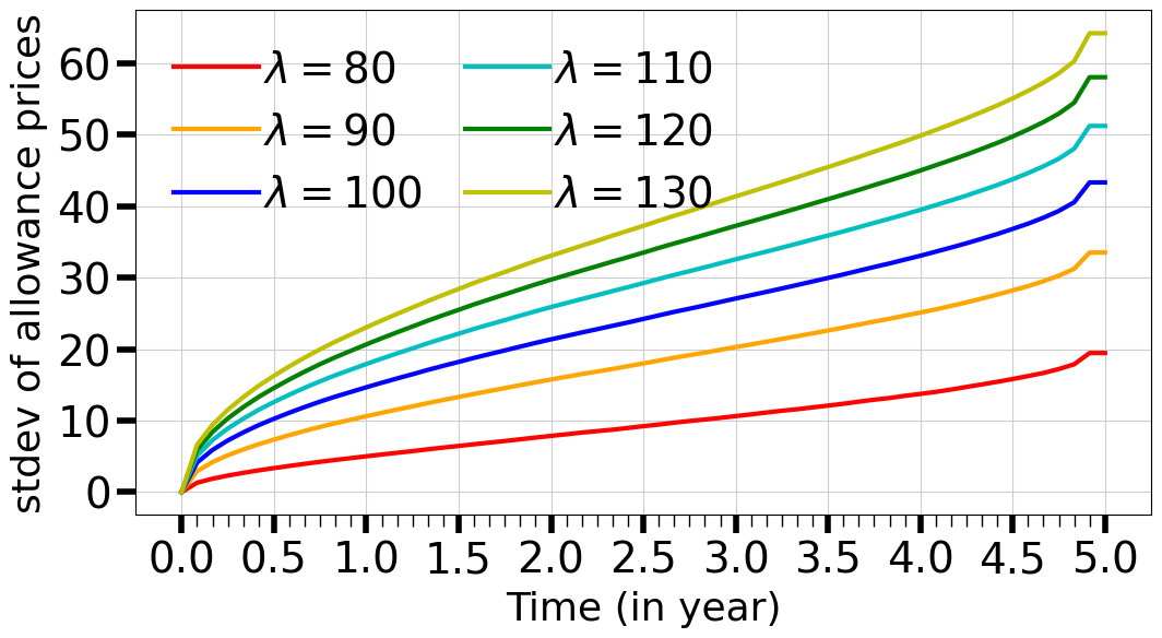
(a) Dependence on $\lambda$.

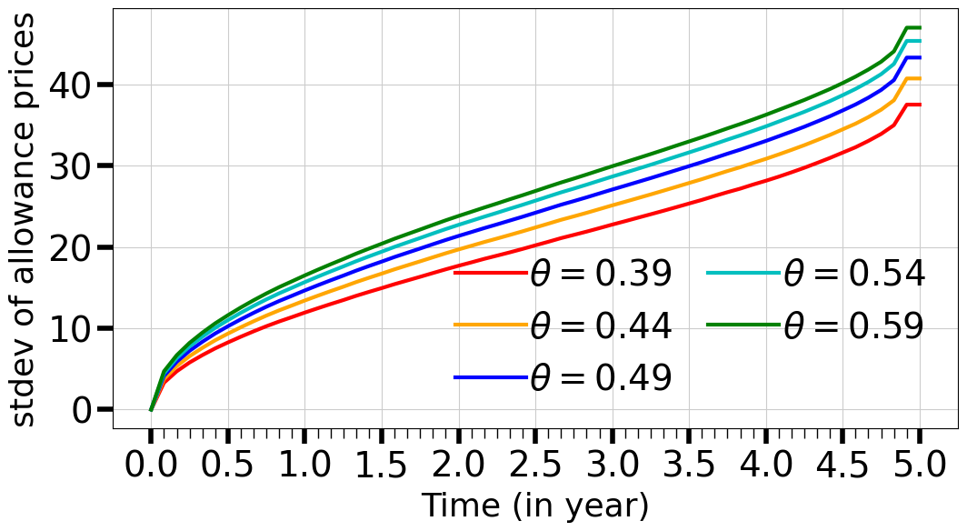
(b) Dependence on $\theta$.

Figure 1. Standard deviations of the allowance prices $\mathbf{P}_{t}$ depending on the penalty $\lambda$ (in € ) and the emission cap $\theta$.

It is also important to stress that $\lambda$ affects not only the average levels of the allowance prices $\mathbf{P}_{t}$, but also their standard deviations: see Figures 11 (a) and 2. In Figure 2, we show how changes in $\lambda$ distort the shape of the distribution of the allowance prices $\mathbf{P}_{t}$. This figure provides the means and quartiles of their distributions over time. In panel (a), the skewness of the distributions ranges from $-1.79$ to $-0.37$, while in panel (b), it ranges from $-0.32$ to $-0.07$. This suggests that the left skewness of the distribution of the prices $\mathbf{P}_{t}$ decreases in $\lambda$. Hence, the likelihood of the allowance prices $\mathbf{P}_{t}$ being greater than the average value $\mathbf{P}_{0}$ decreases as $\lambda$ rises.

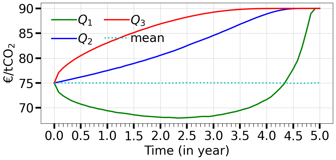
(a) $\lambda=90$€

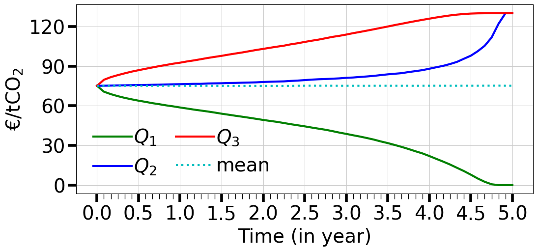
(b) $\lambda=130$€

Figure 2. The first, second, and third quartiles ($Q_{1}$, $Q_{2}$ and $Q_{3}$) and the mean of the allowance prices $\mathbf{P}_{t}$ for two values of the penalty $\lambda$.

5.2. Dependence on the Emissions Cap $\theta$

Future emissions reduction will be achieved by the ETS market through a reduction in the allowances cap $\theta$. The regulator aims for each individual firm $i$ to lower their BAU emissions from $e^{i}_{t}$ to $\theta e^{i}_{t}$ at time $t$.

$\theta$	$0.39$	$0.44$	$0.49$	$0.54$	$0.59$
$\mathrm{EE}(\bm{\alpha})$ ($\mathrm{Gton}$)	$0.0194$	$0.0163$	$0.0137$	$0.0116$	$0.0097$
$\mathbf{P}_{0}$ (€)	$83.00$	$79.02$	$75.04$	$71.06$	$67.08$
$\eta_{\theta}\big{(}\mathbf{P}_{0}\big{)}$	$-0.37$	$-0.44$	$-0.52$	$-0.61$	$-0.70$
$\eta_{\theta}\big{(}\bm{\alpha}^{c}(0)\big{)}$	$-0.59$	$-0.71$	$-0.87$	$-1.05$	$-1.27$
$\eta_{\theta}\big{(}\bm{\alpha}^{c}(1)\big{)}$	$-0.59$	$-0.72$	$-0.88$	$-1.06$	$-1.29$
$\eta_{\theta}\big{(}\bm{\alpha}^{d}(0)\big{)}$	$-0.72$	$-0.90$	$-1.11$	$-1.38$	$-1.74$
$\eta_{\theta}\big{(}\bm{\alpha}^{d}(1)\big{)}$	$-0.71$	$-0.88$	$-1.09$	$-1.36$	$-1.70$

Table 7. The expected excess emissions $\mathrm{EE}(\bm{\alpha})$, the mean of the allowance prices $\mathbf{P}_{0}$, and the elasticities $\eta_{\theta}\big{(}\mathbf{P}_{0}\big{)}$ and $\eta_{\theta}\big{(}\bm{\alpha}^{i}(t)\big{)}$ of $\mathbf{P}_{0}$ and of the optimal abatement plans $\bm{\alpha}^{i}(t)$ with respect to emissions cap $\theta$.

To illustrate how allowance markets are sensitive to $\theta$, we consider a situation where a regulator increases the emissions cap $\theta$ by issuing more allowances. This kind of policy has been implemented in 2023 by the UK to reduce the emissions of the private sector.

The expected excess emissions $\mathrm{EE}(\bm{\alpha})$ decrease as it provides more pollution possibilities for firms, as illustrated in Table 7. In view of Eqn.  (4.4), a rise in $\theta$ leads to a reduction in the expected marginal abatement costs $\bm{\mathrm{MAC}}^{i}(t)$ for firms. Hence, as $\theta$ increases, there is a corresponding reduction in the allowance price $\mathbf{P}_{0}$: see Table 7. This market mechanism is underscored by the negative elasticity between the emission cap $\theta$ and the mean of allowance prices $\mathbf{P}_{0}$. With the rise in $\theta$, the sensitivity of $\mathbf{P}_{0}$ to $\theta$ also grows. Both firms tend to reduce their efforts in emissions reduction as $\theta$ increases, as they are allowed to pollute more without additional effort. The optimal abatement plans $\bm{\alpha}$ shows a high level of elasticities to $\theta$. Due to the higher cost of abatement for firms in the industry sector compared to those in the power sector, their sensitivity of abatement share $\bm{\alpha}^{d}$ is relatively higher in absolute terms.

Figure 11 (b) shows how the standard deviation of the allowance prices $\mathbf{P}_{t}$ increases in $\theta$. To understand why, one can consider the quartiles reported in Figure 3, which shows the shape of the distributions of the allowance prices $\mathbf{P}_{t}$. In the presence of a larger cap, in Figure 33 (b), in some scenarios, one can see that the increase in the price of allowances is less significant as the horizon grows. The reason is that firms are less constrained when the cap is high, so that the allowance price can even fall to zero if the market exhibits an excess of allowances, as underlined by the first quartile $Q_{1}$ at the end of the period.

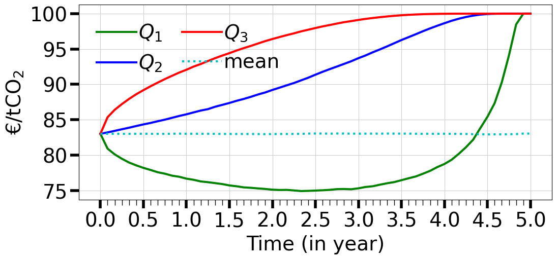
(a) $\theta=0.39$

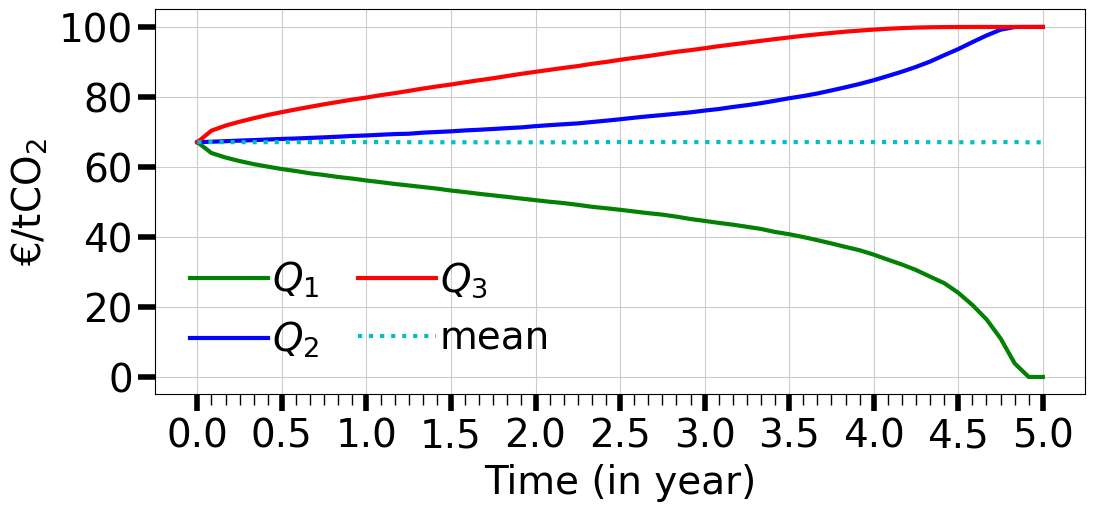
(b) $\theta=0.59$

Figure 3. The first, second, and third quartiles ($Q_{1}$, $Q_{2}$ and $Q_{3}$) and the mean of the allowance prices $\mathbf{P}_{t}$ for two values of emissions cap $\theta$.

5.3. Dependence on the Linear Abatement Cost Coefficient $\mathrm{k}^{c}$

Another key parameter is the cheaper firm linear abatement cost coefficient $\mathrm{k}^{c}$. In general, the abatement cost parameters (liner/quadratic) remain quite uncertain in the literature, as their empirical measurement is difficult. A baseline model for optimal transition is the DICE model from Barrage and Nordhaus (2024). From its first version to the most recent, the backstop price (the abatement cost coefficients in our context) has consistently increased with each revision of DICE. In the latest version, this value has more than doubled, underscoring the uncertainty surrounding this parameter and making it a suitable candidate for robustness analysis. This section evaluates the sensitivity to alternative assumptions regarding $\mathrm{k}^{c}$.

$\mathrm{k}^{c}$ (€)	$20$	$25$	$30$	$35$	$40$
$\mathrm{EE}(\bm{\alpha})$ ($\mathrm{Gton}$)	$0.0171$	$0.0156$	$0.0137$	$0.0114$	$0.0087$
$\mathbf{P}_{0}$ (€)	$69.33$	$72.19$	$75.04$	$77.90$	$80.76$
$\eta_{\mathrm{k}^{c}}\big{(}\mathbf{P}_{0}\big{)}$	$0.16$	$0.20$	$0.23$	$0.26$	$0.28$
$\eta_{\mathrm{k}^{c}}\big{(}\bm{\alpha}^{c}(0)\big{)}$	$-0.17$	$-0.23$	$-0.29$	$-0.35$	$-0.42$
$\eta_{\mathrm{k}^{c}}\big{(}\bm{\alpha}^{c}(1)\big{)}$	$-0.17$	$-0.23$	$-0.28$	$-0.35$	$-0.42$
$\eta_{\mathrm{k}^{c}}\big{(}\bm{\alpha}^{d}(0)\big{)}$	$0.39$	$0.44$	$0.49$	$0.53$	$0.56$
$\eta_{\mathrm{k}^{c}}\big{(}\bm{\alpha}^{d}(1)\big{)}$	$0.38$	$0.44$	$0.48$	$0.52$	$0.55$

Table 8. The expected excess emissions $\mathrm{EE}(\bm{\alpha})$, the mean of the allowance prices $\mathbf{P}_{0}$, and the elasticities $\eta_{\mathrm{k}^{c}}\big{(}\mathbf{P}_{0}\big{)}$ and $\eta_{\mathrm{k}^{c}}\big{(}\bm{\alpha}^{i}(t)\big{)}$ of $\mathbf{P}_{0}$ and of the optimal abatement plans $\bm{\alpha}^{i}(t)$ with respect to the linear abatement cost coefficient $\mathrm{k}^{c}$.

The expected excess emissions $\mathrm{EE}(\bm{\alpha})$ may decline with an increase in $\mathrm{k}^{c}$: see Table 8. The main rationale behind this paradoxical outcome is that both firms are willing to take on a higher level of risk in surpassing the emissions cap when $\mathrm{k}^{c}$ is low. However, for higher values of $\mathrm{k}^{c}$, both firms become more cautious in managing their risk of exceeding the emissions cap, as evidenced by the elasticities $\eta_{\mathrm{k}^{c}}\big{(}\bm{\alpha}^{i}(t)\big{)}$ of their efforts in the table. Nevertheless, if $\lambda$ is low, for instance $\lambda=80$€, we checked that the mitigation effort $\bm{\alpha}^{c}(t)$ of a cheaper firm $c$ becomes highly sensitive to $\mathrm{k}^{c}$, in contrast to the dirty firm’s mitigation effort. Hence, in this case, the expected excess emissions $\mathrm{EE}(\bm{\alpha})$ are increasing in $\mathrm{k}^{c}$, as expected.

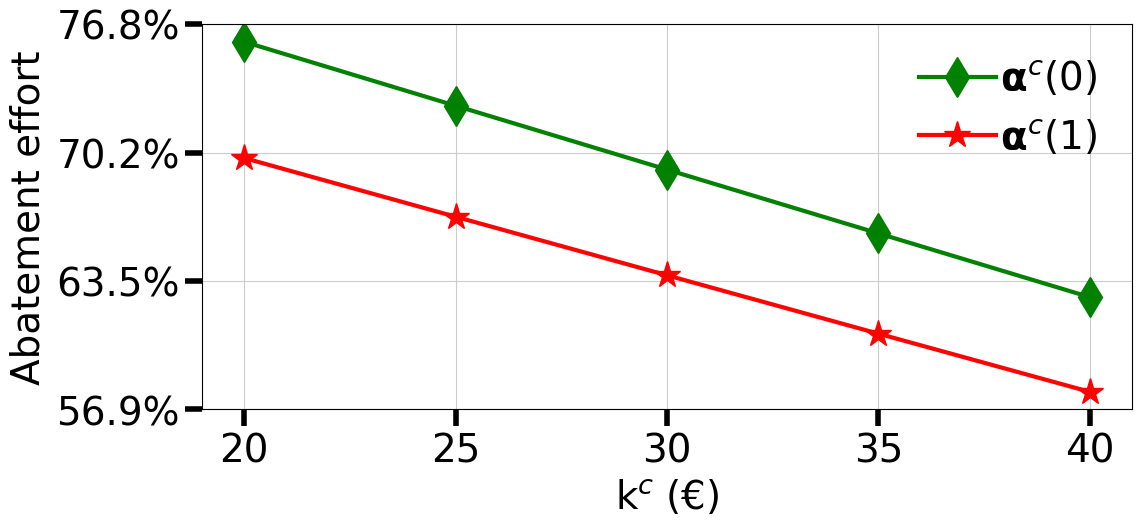
(a) Firm $c$.

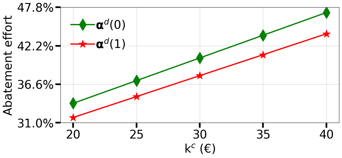
(b) Firm $d$.

Figure 4. Firms optimal abatement plan $\bm{\alpha}^{i}(t)$ as a function of the cheaper firm linear abatement cost coefficient $\mathrm{k}^{c}$.

As the value of $\mathrm{k}^{c}$ grows, the costs borne by firm $c$ for emissions reduction also increase, consequently diminishing the significance of allowance market transactions between the clean and dirty firms. The effort $\bm{\alpha}^{c}(t)$ exerted by firm $c$ to reduce emissions decreases towards the baseline target $1-\theta=0.51$, as shown in Figure 44 (a). In contrast, firm $d$ increases its effort $\bm{\alpha}^{d}(t)$ to meet the same target, as the gain from purchasing allowances from the clean sector reduces, as depicted in Figure 44 (b).

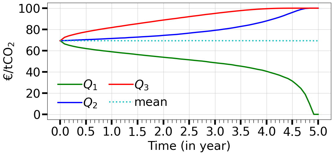
(a) $\mathrm{k}^{c}=20$ €.

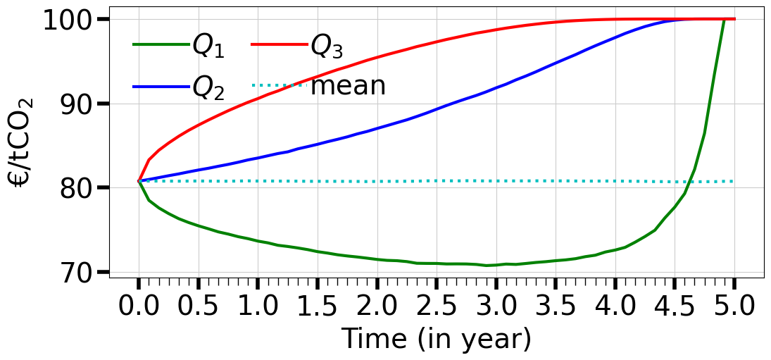
(b) $\mathrm{k}^{c}=40$ €.

Figure 5. The first, second, and third quartiles ($Q_{1}$, $Q_{2}$ and $Q_{3}$) and the mean of the allowance prices $\mathbf{P}_{t}$ for two values of the linear abatement cost coefficient $\mathrm{k}^{c}$.

The market of allowances clears by an increase in the mean of the allowance price $\mathbf{P}_{0}$ as $\mathrm{k}^{c}$ rise: see Table 8. Figure 5 also provides the means and quartiles of the distributions of the allowance prices $\mathbf{P}_{t}$ over time. In panel (a), the left skewness of the distributions increases from $-0.19$ to $-0.84$ as time progress, while in panel (b), it increases from $-0.33$ to $-1.56$. This suggest that the distribution of $\mathbf{P}_{t}$ skews more to the left as $\mathrm{k}^{c}$ increases. This occurs because the supply of permits from firm $c$ on the market becomes larger for low $\mathrm{k}^{c}$, potentially driving the allowance price to zero if the number of permits exceeds the cap before the compliance period. In contrast, for higher $\mathrm{k}^{c}$ the gain from trading between the two firms diminishes significantly. Both firms struggle to sufficiently reduce their emissions, causing the allowance price to increase, until it would reach $\lambda$. For relatively higher value of $\mathrm{k}^{c}$, the economy also experiences permit shortages, and resulting in lower price volatility. Hence, an inverse relationship exists between $\mathrm{k}^{c}$ and allowance price volatility: see Figure 66 (a).

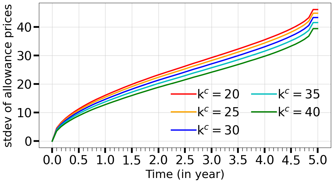
(a) Dependence on $\mathrm{k}^{c}$.

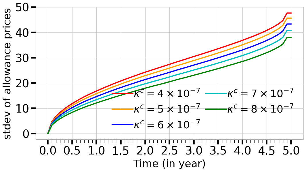
(b) Dependence on $\kappa^{c}$.

Figure 6. The standard deviation of the allowance prices $\mathbf{P}_{t}$ for different values of the linear $\mathrm{k}^{c}$ (in €$/\mathrm{ton}$) and quadratic $\kappa^{c}$ (in €$/\mathrm{ton}^{2}$) abatement cost coefficients.

5.4. Dependence on the Linear Abatement Cost Coefficient $\mathrm{k}^{d}$

Let us now turn to the cost parameter $\mathrm{k}^{d}$ of the dirty firm. Since the results are quite similar to those for $\mathrm{k}^{c}$, we focus only on the differences, which are highlighted in Table 9.

$\mathrm{k}^{d}$ (€)	$30$	$35$	$40$	$45$	$50$
$\mathrm{EE}(\bm{\alpha})$ ($\mathrm{Gton}$)	$0.0064$	$0.0099$	$0.0137$	$0.0180$	$0.0229$
$\mathbf{P}_{0}$ (€)	$70.78$	$72.92$	$75.04$	$77.16$	$79.27$
$\eta_{\mathrm{k}^{d}}\big{(}\mathbf{P}_{0}\big{)}$	$0.18$	$0.20$	$0.23$	$0.25$	$0.27$
$\eta_{\mathrm{k}^{d}}\big{(}\bm{\alpha}^{c}(0)\big{)}$	$0.32$	$0.35$	$0.38$	$0.40$	$0.43$
$\eta_{\mathrm{k}^{d}}\big{(}\bm{\alpha}^{c}(1)\big{)}$	$0.32$	$0.35$	$0.38$	$0.41$	$0.43$
$\eta_{\mathrm{k}^{d}}\big{(}\bm{\alpha}^{d}(0)\big{)}$	$-0.42$	$-0.53$	$-0.66$	$-0.81$	$-0.99$
$\eta_{\mathrm{k}^{d}}\big{(}\bm{\alpha}^{d}(1)\big{)}$	$-0.42$	$-0.53$	$-0.65$	$-0.80$	$-0.98$

Table 9. The expected excess emissions $\mathrm{EE}(\bm{\alpha})$, the mean of the allowance prices $\mathbf{P}_{0}$, and the elasticities $\eta_{\mathrm{k}^{d}}\big{(}\mathbf{P}_{0}\big{)}$ and $\eta_{\mathrm{k}^{d}}\big{(}\bm{\alpha}^{i}(t)\big{)}$ of $\mathbf{P}_{0}$ and of the optimal abatement plans $\bm{\alpha}^{i}(t)$ with respect to the dirty firm linear abatement cost coefficient $\mathrm{k}^{d}$.

An increase in $\mathrm{k}^{d}$ leads to a higher demand for permit trading with the clean sector. As the gap between $\mathrm{k}^{c}$ and $\mathrm{k}^{d}$ widens, the potential gains from trading between the two sectors increase. Hence, the abatement plans of the clean and dirty firms have elasticities with respect to $\mathrm{k}^{d}$ of opposite signs. As $\mathrm{k}^{d}$ gets higher, the dirty firm prefer to pay the penalty instead of abating, which leads to an increase in the expected excess emission.

5.5. Dependence on the Quadratic Abatement Cost Coefficient $\kappa^{c}$

This section investigates how the convexity abatement cost coefficient $\kappa^{c}$ of the clean firm affects the equilibrium patterns.

$\kappa^{c}$ (€/$\mathrm{ton}^{2}$)	$4\times 10^{-7}$	$5\times 10^{-7}$	$6\times 10^{-7}$	$7\times 10^{-7}$	$8\times 10^{-7}$
$\mathrm{EE}(\bm{\alpha})$ ($\mathrm{Gton}$)	$0.0188$	$0.0166$	$0.0137$	$0.0104$	$0.0067$
$\mathbf{P}_{0}$ (€)	$65.12$	$70.46$	$75.04$	$79.03$	$82.52$
$\eta_{\kappa^{c}}\big{(}\mathbf{P}_{0}\big{)}$	$0.35$	$0.35$	$0.34$	$0.33$	$0.32$
$\eta_{\kappa^{c}}\big{(}\bm{\alpha}^{c}(0)\big{)}$	$-0.34$	$-0.39$	$-0.43$	$-0.47$	$-0.50$
$\eta_{\kappa^{c}}\big{(}\bm{\alpha}^{c}(1)\big{)}$	$-0.33$	$-0.38$	$-0.42$	$-0.46$	$-0.49$
$\eta_{\kappa^{c}}\big{(}\bm{\alpha}^{d}(0)\big{)}$	$0.92$	$0.81$	$0.73$	$0.67$	$0.62$
$\eta_{\kappa^{c}}\big{(}\bm{\alpha}^{d}(1)\big{)}$	$0.90$	$0.80$	$0.72$	$0.66$	$0.61$

Table 10. The expected excess emissions $\mathrm{EE}(\bm{\alpha})$, the mean of the allowance prices $\mathbf{P}_{0}$, and the elasticities $\eta_{\kappa^{c}}\big{(}\mathbf{P}_{0}\big{)}$ and $\eta_{\kappa^{c}}\big{(}\bm{\alpha}^{i}(t)\big{)}$ of $\mathbf{P}_{0}$ and of the optimal abatement plans $\bm{\alpha}^{i}(t)$ with respect to the quadratic abatement cost coefficient $\kappa^{c}$.

The impact on firms’ abatement plans and on allowance prices is quite similar to the influence of the linear cost coefficient $\mathrm{k}^{c}$, as shown in Table 10. The abatement plans of the dirty firm appear more sensitive to $\kappa^{c}$ than the ones of the clean firm. Indeed, the dirty firm must compensate for the reduction in permit availability by increasing its abatement efforts, as shown in Table 10. The firm $c$ gradually decreases its optimal abatement plan $\bm{\alpha}^{c}(t)$ towards the baseline target $1-\theta$; the allowance become more expensive and hence firm $d$ increases its efforts $\bm{\alpha}^{d}(t)$ to meet the same target of $0.51$. The elasticity of firm $d$’s optimal abatement plan to $\kappa^{c}$ appears greater than the one of firm $c$: see Table 10.

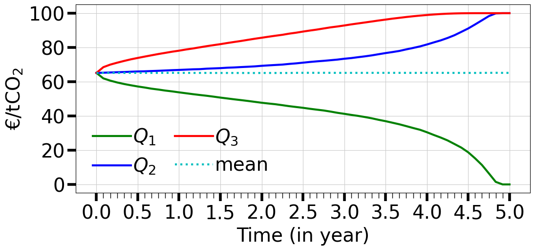
(a) $\kappa^{c}=4\times 10^{-7}$€$/\mathrm{ton}^{2}$

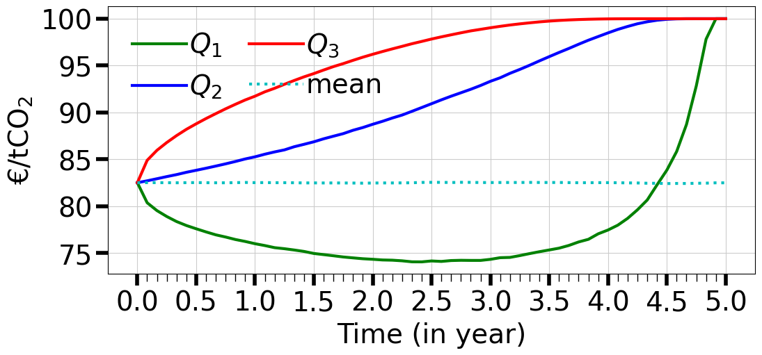
(b) $\kappa^{c}=8\times 10^{-7}$€$/\mathrm{ton}^{2}$

Figure 7. The first, second, and third quartiles ($Q_{1}$, $Q_{2}$ and $Q_{3}$) and the mean of the allowance prices $\mathbf{P}_{t}$ for two values of the quadratic abatement cost coefficient $\kappa^{c}$.

As visible in Figure 77 (a), a low $\kappa^{c}$ can potentially lead to an oversupply of permits by the clean firm, resulting in some realizations of the allowance price in the lower tail (Q1) where the market price is very low or even zero. Conversely, in less favorable states of nature (Q3), the supply of permits is depleted faster than expected, forcing firms to exceed the cap and pay penalty. In contrast, as shown in Figure 77 (b), when abatement costs are more convex, the supply of permits by the clean firm is lower. The market is then severely constrained by this limited supply, causing the permit price to equal the penalty price across all realizations of the stochastic variables. For the same reason as in the case of the linear abatement cost parameter $\mathrm{k}^{c}$, an inverse relationship exists between $\kappa^{c}$ and the standard deviations of the allowance prices: see Figure 66 (b).

5.6. Dependence on the Quadratic Abatement Cost Coefficient $\kappa^{d}$

The cost parameter $\kappa^{d}$ has an effect on both firms’ optimal abatement plans and allowance prices similar to $\kappa^{c}$. In this section, we focus specifically on the differences, which are highlighted in Table 11.

An increase in the cost parameter $\kappa^{d}$ leads to additional demand for trading permits from the dirty firm. In response to this increased demand, the clean firm raises its optimal abatement plan, as shown in Table 11. As highlighted by the elasticities, abatements tend to respond more strongly in the dirty sector, which directly experiences the effects of a change in $\kappa^{d}$. The increased demand for allowances from the dirty firm is cleared by the market through a relative rise in the price of allowances. However, as the market becomes more tense, excess emissions also increase in $\kappa^{d}$.

$\kappa^{d}$ (€/$\mathrm{ton}^{2}$)	$6\times 10^{-7}$	$7\times 10^{-7}$	$8\times 10^{-7}$	$9\times 10^{-7}$	$1\times 10^{-6}$
$\mathrm{EE}(\bm{\alpha})$ ($\mathrm{Gton}$)	$0.0062$	$0.0100$	$0.0137$	$0.0173$	$0.0206$
$\mathbf{P}_{0}$ (€)	$70.63$	$73.01$	$75.04$	$76.79$	$78.32$
$\eta_{\kappa^{d}}\big{(}\mathbf{P}_{0}\big{)}$	$0.22$	$0.21$	$0.20$	$0.19$	$0.18$
$\eta_{\kappa^{d}}\big{(}\bm{\alpha}^{c}(0)\big{)}$	$0.38$	$0.36$	$0.33$	$0.31$	$0.30$
$\eta_{\kappa^{d}}\big{(}\bm{\alpha}^{c}(1)\big{)}$	$0.38$	$0.36$	$0.34$	$0.32$	$0.30$
$\eta_{\kappa^{d}}\big{(}\bm{\alpha}^{d}(0)\big{)}$	$-0.49$	$-0.54$	$-0.57$	$-0.60$	$-0.63$
$\eta_{\kappa^{d}}\big{(}\bm{\alpha}^{d}(1)\big{)}$	$-0.51$	$-0.55$	$-0.58$	$-0.61$	$-0.63$

Table 11. The expected excess emissions $\mathrm{EE}(\bm{\alpha})$, the mean of the allowance prices $\mathbf{P}_{0}$, and the elasticities $\eta_{\kappa^{d}}\big{(}\mathbf{P}_{0}\big{)}$ and $\eta_{\kappa^{d}}\big{(}\bm{\alpha}^{i}(t)\big{)}$ of $\mathbf{P}_{0}$ and of the optimal abatement plans $\bm{\alpha}^{i}(t)$ with respect to the quadratic abatement cost coefficient $\kappa^{d}$.

5.7. Dependence on the Mean $\bar{\mu}$ of the Aggregate BAU Emissions

This section analyzes the impacts of a change in the mean $\bar{\mu}$ of the business-as-usual (BAU) emissions, as described in Eqn.  (4.5). An increase in $\bar{\mu}$ results in firms facing higher costs for abatement. Consequently, the clean firm reduces its abatement efforts towards the baseline target $1-\theta=0.51$ and offers a smaller quantity of allowances in the market: see Figure 88 (a).

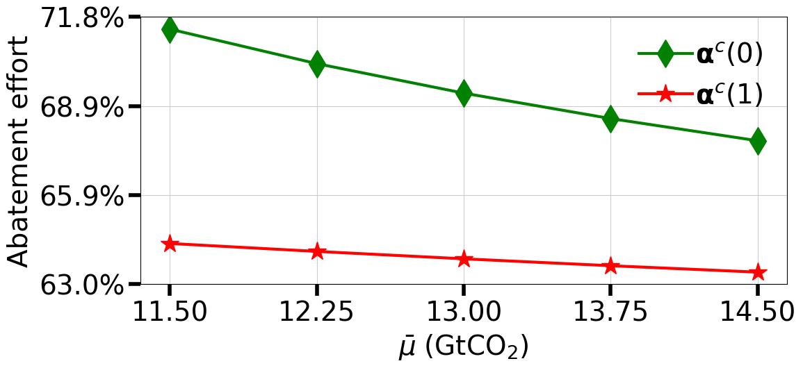
(a) Firm $c$.

(b) Firm $d$.

Figure 8. Firms optimal abatement plan $\bm{\alpha}^{i}(t)$ as a function of mean $\bar{\mu}$ of the aggregate BAU emissions.

This outcome is somewhat unexpected for the clean firm, as one could expect an increase in abatement efforts to counter the escalating emissions. The dirty firm, on the other hand, decreases its abatement efforts initially at time $0$ and subsequently intensifies its efforts towards the same target of $0.51$ as $\bar{\mu}$ rises, as depicted in Figure 88 (b). Hence, the expected excess emission $\mathrm{EE}(\bm{\alpha})$ is increasing in $\bar{\mu}$: see Table 12, which also shows that the market responds to an increase in $\bar{\mu}$ by clearing at a higher mean of the allowances prices $\mathbf{P}_{0}$.

$\bar{\mu}$ ($\mathrm{Gton}$)	$11.5$	$12.25$	$13.00$	$13.75$	$14.50$
$\mathrm{EE}(\bm{\alpha})$ ($\mathrm{Gton}$)	$0.0128$	$0.0132$	$0.0137$	$0.0143$	$0.0149$
$\mathbf{P}_{0}$ (€)	$71.06$	$73.04$	$75.04$	$77.06$	$79.10$
$\eta_{\bar{\mu}}\big{(}\mathbf{P}_{0}\big{)}$	$0.42$	$0.45$	$0.46$	$0.48$	$0.50$
$\eta_{\bar{\mu}}\big{(}\bm{\alpha}^{c}(0)\big{)}$	$-0.27$	$-0.24$	$-0.23$	$-0.21$	$-0.19$
$\eta_{\bar{\mu}}\big{(}\bm{\alpha}^{c}(1)\big{)}$	$-0.06$	$-0.06$	$-0.06$	$-0.06$	$-0.06$
$\eta_{\bar{\mu}}\big{(}\bm{\alpha}^{d}(0)\big{)}$	$-0.03$	$-0.01$	$-0.00$	$0.00$	$0.01$
$\eta_{\bar{\mu}}\big{(}\bm{\alpha}^{d}(1)\big{)}$	$0.12$	$0.12$	$0.11$	$0.11$	$0.11$

Table 12. The expected excess emissions $\mathrm{EE}(\bm{\alpha})$, the mean of the allowance prices $\mathbf{P}_{0}$, and the elasticities $\eta_{\bar{\mu}}\big{(}\mathbf{P}_{0}\big{)}$ and $\eta_{\bar{\mu}}\big{(}\bm{\alpha}^{i}(t)\big{)}$ of $\mathbf{P}_{0}$ and of the optimal abatement plans $\bm{\alpha}^{i}(t)$ with respect to the mean $\bar{\mu}$ of the aggregate BAU emissions.

Figure 99 (a) displays the inverse relationship exists between $\bar{\mu}$ and the standard deviations of the allowance prices $\mathbf{P}_{t}$. Figure 10 provides the means and quartiles of the distributions of the allowance prices $\mathbf{P}_{t}$ over time. The patterns of the Figures 7 and 10 are similar. A comparable rationale can be applied to explain the impact of $\bar{\mu}$ on the volatility of allowance prices, akin to the argument presented for the abatement cost coefficients $\mathrm{k}^{c}$ and $\kappa^{c}$ of the clean firm in Sections 5.3 and 5.5.

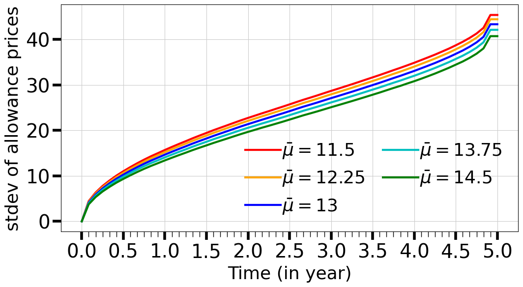
(a) Dependence on $\bar{\mu}$ .

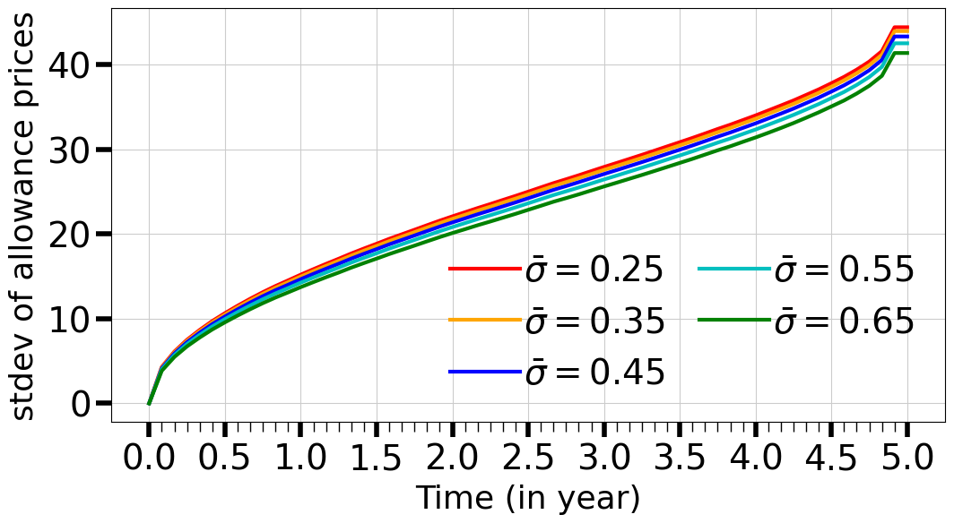
(b) Dependence on $\bar{\sigma}$.

Figure 9. The standard deviation of the allowance prices $\mathbf{P}_{t}$ for different values of a mean $\bar{\mu}$ and a standard deviation $\bar{\sigma}$ of the aggregate BAU emissions (in $\mathrm{Gton}$).

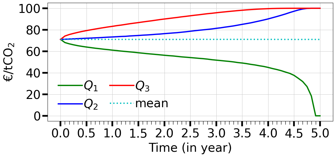
(a) $\bar{\mu}=11.5\mathrm{Gton}$.

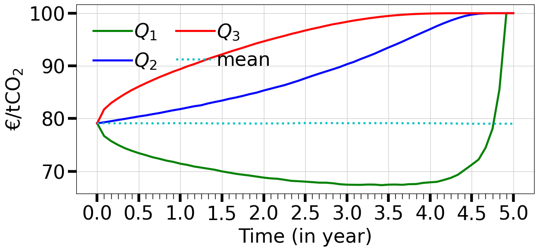
(b) $\bar{\mu}=14.5\mathrm{Gton}$.

Figure 10. The first, second, and third quartiles ($Q_{1}$, $Q_{2}$ and $Q_{3}$) and the mean of the allowance prices $\mathbf{P}_{t}$ for two values of the mean $\bar{\mu}$ of aggregate BAU emissions.

5.8. Dependence on the Standard Deviation $\bar{\sigma}$ of the Aggregate BAU Emissions

We now evaluate the impacts of a change in the volatility $\bar{\sigma}$ of BAU emissions. The latter provides a measure of uncertainty that firms have to deal with along the transition up to the compliance period.

As shown in Table 13, an increase in $\bar{\sigma}$ raises the expected excess emissions $\mathrm{EE}(\bm{\alpha})$, as firms must cope with larger, unexpected fluctuations, increasing the likelihood of exceeding the cap. In response to this heightened risk of exceeding the cap and incurring penalty, the mean allowance price $\mathbf{P}_{0}$ rises accordingly. Nevertheless, the responsiveness of $\mathbf{P}_{0}$ to $\bar{\sigma}$ appears to be minimal.

$\bar{\sigma}$ ($\mathrm{Gton}$)	$0.25$	$0.35$	$0.45$	$0.55$	$0.65$
$\mathrm{EE}(\bm{\alpha})$ ($\mathrm{Gton}$)	$0.0075$	$0.0105$	$0.0137$	$0.0171$	$0.0208$
$\mathbf{P}_{0}$ (€)	$73.06$	$73.91$	$75.04$	$76.45$	$78.12$
$\eta_{\bar{\sigma}}\big{(}\mathbf{P}_{0}\big{)}$	$0.03$	$0.05$	$0.08$	$0.11$	$0.14$
$\eta_{\bar{\sigma}}\big{(}\bm{\alpha}^{c}(0)\big{)}$	$0.05$	$0.08$	$0.13$	$0.18$	$0.23$
$\eta_{\bar{\sigma}}\big{(}\bm{\alpha}^{c}(1)\big{)}$	$-0.06$	$-0.08$	$-0.10$	$-0.12$	$-0.13$
$\eta_{\bar{\sigma}}\big{(}\bm{\alpha}^{d}(0)\big{)}$	$0.06$	$0.11$	$0.16$	$0.23$	$0.29$
$\eta_{\bar{\sigma}}\big{(}\bm{\alpha}^{d}(1)\big{)}$	$0.09$	$0.13$	$0.16$	$0.18$	$0.20$

Table 13. The expected excess emissions $\mathrm{EE}(\bm{\alpha})$, the mean of the allowance prices $\mathbf{P}_{0}$, and the elasticities $\eta_{\bar{\sigma}}\big{(}\mathbf{P}_{0}\big{)}$ and $\eta_{\bar{\sigma}}\big{(}\bm{\alpha}^{i}(t)\big{)}$ of $\mathbf{P}_{0}$ and of the optimal abatement plans $\bm{\alpha}^{i}(t)$ with respect to standard deviation $\bar{\sigma}$ of the aggregate BAU emissions.

Using Eqn. (3.13), for each $i$ in $\{c,d\}$, the expected abatement cost is simplified to

$$\begin{cases}\mathrm{k}^{i}\alpha^{i}(0)\mu+\frac{\kappa^{i}}{2}\big{(}\alpha^{i}(0)\mu\big{)}^{2}&t=0\\ \mathrm{k}^{i}\alpha^{i}(t)\mu+\frac{\kappa^{i}}{2}\big{(}\alpha^{i}(t)\mu\big{)}^{2}+\big{(}\alpha^{i}(t)\sigma\big{)}^{2}&t>0,\end{cases}$$

where $\mu$ and $\sigma$ are given as a function of $\bar{\mu}$ and $\bar{\sigma}$ in (4.5). As a result, the expected abatement costs at time $t=0$ do not depend on $\bar{\sigma}$, whereas expected abatement costs at later times $t>0$ are increasing in $\bar{\sigma}$ and greater than the time $0$ costs. Hence, an increase in $\bar{\sigma}$ makes abatement cheaper at time $0$ relative to the later times $t>0$. Therefore, the abatement efforts of both firms at time $0$ increase in $\bar{\sigma}$ (see the sign of $\eta_{\bar{\sigma}}\big{(}\bm{\alpha}^{i}(t)\big{)}$ in Table 13 ). The table also shows, at time 1 and beyond, as $\bar{\sigma}$ increases, the abatement effort $\bm{\alpha}^{c}(t)$ of the clean firm declines, while the dirty firm intensifies its efforts $\bm{\alpha}^{d}(t)$ until it reaches to the target of $1-\theta$.

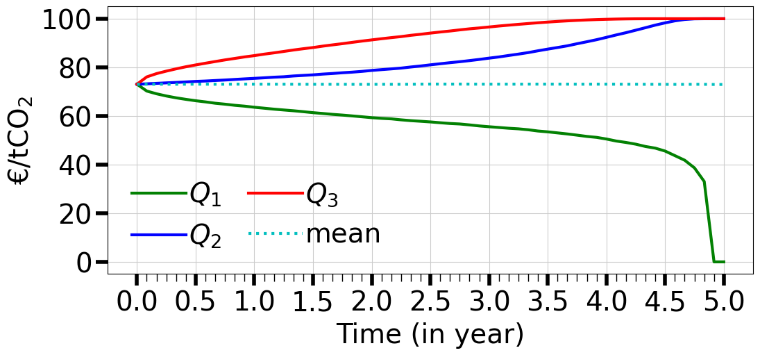
(a) $\bar{\sigma}=0.25\mathrm{Gton}$.

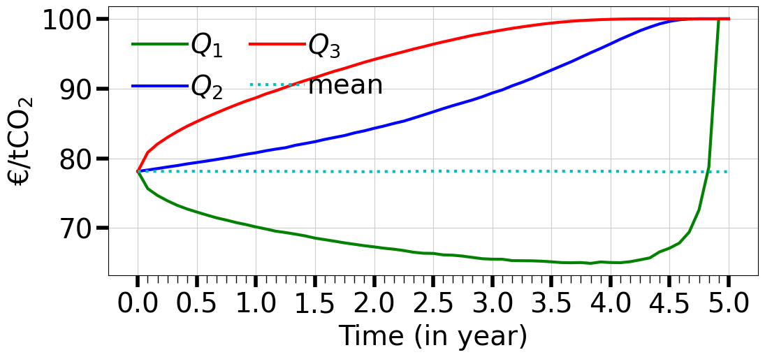
(b) $\bar{\sigma}=0.65\mathrm{Gton}$.

Figure 11. The first, second, and third quartiles ($Q_{1}$, $Q_{2}$ and $Q_{3}$) and the mean of the allowance prices $\mathbf{P}_{t}$ for two values of the standard deviation $\bar{\sigma}$ of the aggregate BAU emissions.

The standard deviations of the allowance prices $\mathbf{P}_{t}$ are (very slowly) decreasing in $\bar{\sigma}$, see Figure 99 (b). This finding contrasts with the results of Seifert et al. (2008), which suggest that an increase in $\bar{\sigma}$ leads to higher volatility in allowance prices. The patterns shown in Figures 7, 10 and 11 are similar. A comparable rationale can be applied to explain the impact of $\bar{\sigma}$ on the volatility of allowance prices, akin to the argument presented in Sections 5.3, 5.5 and 5.7.

5.9. Dependence on the Coefficient of Correlation $\rho$ between Firms Emissions

The final parameter we analyze is the correlation coefficient $\rho$ between emission shocks across the two firms. Table 14 presents the impact of an increase in $\rho$.

$\rho$	$0.71$	$0.78$	$0.85$	$0.92$	$0.99$
$\mathrm{EE}(\bm{\alpha})$ ($\mathrm{Gton}$)	$0.0197$	$0.0169$	$0.0137$	$0.0099$	$0.0035$
$\mathbf{P}_{0}$ (€)	$75.28$	$75.15$	$75.04$	$74.94$	$74.80$
$\sigma_{\mathbf{P}_{T}}$	$43.14$	$43.21$	$43.28$	$43.34$	$43.41$
$\eta_{\rho}\big{(}\mathbf{P}_{0}\big{)}$	$-0.02$	$-0.02$	$-0.02$	$-0.02$	$-0.06$
$\eta_{\rho}\big{(}\bm{\alpha}^{c}(0)\big{)}$	$-0.03$	$-0.03$	$-0.03$	$-0.03$	$-0.10$
$\eta_{\rho}\big{(}\bm{\alpha}^{c}(1)\big{)}$	$0.02$	$0.02$	$0.03$	$0.04$	$0.10$
$\eta_{\rho}\big{(}\bm{\alpha}^{d}(0)\big{)}$	$-0.04$	$-0.04$	$-0.04$	$-0.04$	$-0.13$
$\eta_{\rho}\big{(}\bm{\alpha}^{d}(1)\big{)}$	$-0.02$	$-0.02$	$-0.03$	$-0.04$	$-0.11$

Table 14. The expected excess emissions $\mathrm{EE}(\bm{\alpha})$, the mean of the allowance prices $\mathbf{P}_{0}$, the standard deviation $\sigma_{\mathbf{P}_{T}}$ of the price $\mathbf{P}_{T}$, and the elasticities $\eta_{\rho}\big{(}\mathbf{P}_{0}\big{)}$ and $\eta_{\rho}\big{(}\bm{\alpha}^{i}(t)\big{)}$ of $\mathbf{P}_{0}$ and of the optimal abatement plans $\bm{\alpha}^{i}(t)$ with respect to the coefficient of correlation $\rho$ between firms emission.

It is worth noting that the magnitude of the effects is relatively small, despite the significant increase in $\rho$. A higher correlation implies that when emissions rise in one firm, the other firm experiences similar dynamics. As a result, neither sector can provide a form of insurance to the other. Therefore, as $\rho$ increases, the mutual insurance mechanism between firms is reduced. The clean firm reduces its abatement, but the effect on the allowance price is however quantitatively small.

6. Conclusion

In this paper, we investigate the impact of key factors on the prices of allowances and the mitigation efforts of firms in reducing emissions. We extend the standard cap and trade model in a Gaussian framework that internally calculates allowance prices, trading strategies, and firms’ emission reduction endeavors through Radner equilibrium. An explicit formula is established to determine the price of allowances and its variance. These formulas clearly illustrate how parameters influence the price of allowances. Furthermore, it allows for a sensitivity analysis based on the implicit function theorem to investigate the elasticity of firms’ abatement efforts and the expected allowance price in relation to the fundamental parameters.

The sensitivity analysis results in our model are important for both regulatory bodies and polluters in gaining a deeper understanding of the extent to which firms engage in initiatives aimed at reducing emissions, as well as how changes in input variables affect allowance prices. While our findings are grounded in a Gaussian, risk-neutral framework, future research could explore models that account for varying risk preferences and baseline emissions distribution, potentially enriching the applicability of this work in diverse market settings.

Appendix A Proof of Proposition 2.2

Let $\mathbf{P}$, $\bm{\alpha}$ and $(\mathbf{Q}^{i})_{i}$ be a Radner equilibrium. If $\mathbf{P}$ is not a martingale, then $\mathbb{E}[\Delta\mathbf{P}_{t}1_{B}]>0$ or $<0$ holds for some $t\in 0\,..\,T-1$ and $B\in\mathfrak{F}_{t}$ with $\mathbb{P}[B]>0$. Assuming $\mathbb{E}[\Delta\mathbf{P}_{t}1_{B}]>0$, for $\hat{Q}^{i}_{s}=\mathbf{Q}^{i}_{s}$, $s\neq t$, and $\hat{Q}^{i}_{t}=\mathbf{Q}^{i}_{t}+\bm{1}_{B}$, we obtain

$$\mathbb{E}\big{[}C^{i,\mathbf{P}}(\bm{\alpha}^{i},\hat{Q}^{i})\big{]}=\mathbb{E}\big{[}C^{i,\mathbf{P}}(\bm{\alpha}^{i},\mathbf{Q}^{i})\big{]}-\mathbb{E}[\Delta\mathbf{P}_{t}1_{B}]<\mathbb{E}\big{[}C^{i,\mathbf{P}}(\bm{\alpha}^{i},\mathbf{Q}^{i})\big{]},$$

which contradicts (2.7). If instead $\mathbb{E}[\Delta\mathbf{P}_{t}1_{B}]<0$, using $\hat{Q}^{i}_{s}=\mathbf{Q}^{i}_{s}$, $s\neq t$, $\hat{Q}^{i}_{t}=\mathbf{Q}^{i}_{t}-\bm{1}_{B}$ entails likewise a contradiction to (2.7). Hence $\mathbf{P}$ is martingale.

Observe that $\mathbf{Q}^{i}_{T}$ almost surely coincides with some minimizer of

$$\mathbb{R}\ni x\stackrel{{\scriptstyle g^{i,\bm{\alpha}^{i}}_{\omega}}}{{\mapsto}}x\mathbf{P}_{T}(\omega)+\lambda\big{(}E^{i,\bm{\alpha}^{i}}_{T}(\omega)-A^{i}_{T}(\omega)-x\big{)}^{+}.$$ (A.1)

By convexity of $g^{i,\bm{\alpha}^{i}}_{\omega}$, $0\in\partial g^{i,\bm{\alpha}^{i}}_{\omega}(\mathbf{Q}^{i}_{T})=\big{[}\big{(}g^{i,\bm{\alpha}^{i}}_{\omega}\big{)}^{\prime}_{-}(\mathbf{Q}^{i}_{T}),\big{(}g^{i,\bm{\alpha}^{i}}_{\omega}\big{)}^{\prime}_{+}(\mathbf{Q}^{i}_{T})\big{]}$ holds where $\big{(}g^{i,\bm{\alpha}^{i}}_{\omega}\big{)}^{\prime}_{-}$ and $\big{(}g^{i,\bm{\alpha}^{i}}_{\omega}\big{)}^{\prime}_{+}$ are the left and right hand derivatives of $g^{i,\bm{\alpha}^{i}}_{\omega}$, i.e.

$$\lambda\;\bm{1}_{\big{(}-\infty,\;E^{i,\bm{\alpha}^{i}}_{T}-A^{i}_{T}\big{)}}\big{(}\mathbf{Q}^{i}_{T}\big{)}\leq\mathbf{P}_{T}\leq\lambda\;\bm{1}_{\big{(}-\infty,\;E^{i,\bm{\alpha}^{i}}_{T}-A^{i}_{T}\big{]}}\big{(}\mathbf{Q}^{i}_{T}\big{)}.$$

As a result, $\mathbf{P}_{T}\in[0,\lambda]$. Also using the clearing condition (2.8), we obtain

$$\big{\{}\mathbf{P}_{T}\in(0,\lambda]\big{\}}\subseteq\cap_{i}\Big{\{}\mathbf{Q}^{i}_{T}\leq E^{i,\bm{\alpha}^{i}}_{T}-A^{i}_{T}\Big{\}}\subseteq\big{\{}0\leq E^{\bm{\alpha}}_{T}-A_{T}\big{\}}$$ (A.2)

and

$$\big{\{}\mathbf{P}_{T}\in[0,\lambda)\big{\}}\subseteq\cap_{i}\Big{\{}\mathbf{Q}^{i}_{T}\geq E^{i,\bm{\alpha}^{i}}_{T}-A^{i}_{T}\Big{\}}\subseteq\big{\{}0\geq E^{\bm{\alpha}}_{T}-A_{T}\big{\}}.$$ (A.3)

By (A.2), $\big{\{}\mathbf{P}_{T}\in(0,\lambda]\big{\}}\cap\big{\{}E^{\bm{\alpha}}_{T}-A_{T}<0\big{\}}=\emptyset$, i.e. $\big{\{}E^{\bm{\alpha}}_{T}-A_{T}<0\big{\}}\subseteq\big{\{}\mathbf{P}_{T}=0\big{\}}$. Likewise (A.3) yields $\big{\{}E^{\bm{\alpha}}_{T}-A_{T}>0\big{\}}\subseteq\big{\{}\mathbf{P}_{T}=\lambda\big{\}}$. This together with Assumption 2.2 implies $\mathbf{P}_{T}=\xi^{\bm{\alpha}}$. Hence $\mathbf{P}$ is a martingale closed by $\xi^{\bm{\alpha}}$. Application of (2.11) yields (2.13).

References

Ackerman and
Bueno (2011)
Ackerman, F. and R. Bueno (2011).
Use of McKinsey abatement cost curves for climate economics
modeling.
Stockholm Environment Institute.
Aïd and
Biagini (2023)
Aïd, R. and S. Biagini (2023).
Optimal dynamic regulation of carbon emissions market.
Mathematical Finance33(1), 80–115.
Barrage and
Nordhaus (2024)
Barrage, L. and W. Nordhaus (2024).
Policies, projections, and the social cost of carbon: Results from
the DICE-2023 model.
Proceedings of the National Academy of Sciences of the United
States of America121(13), e2312030121.
Blanchard
et al. (2023)
Blanchard, O., C. Gollier, and J. Tirole (2023).
The portfolio of economic policies needed to fight climate change.
Annual Review of Economics15(Volume 15, 2023),
689–722.
Carmona
et al. (2009)
Carmona, R., M. Fehr, and J. Hinz (2009).
Optimal stochastic control and carbon price formation.
SIAM Journal on Control and Optimization48(4),
2168–2190.
Carmona
et al. (2010)
Carmona, R., M. Fehr, J. Hinz, and A. Porchet (2010).
Market design for emission trading schemes.
SIAM Review52(3), 403–452.
Hitzemann and
Uhrig-Homburg (2018)
Hitzemann, S. and M. Uhrig-Homburg (2018).
Equilibrium price dynamics of emission permits.
Journal of Financial and Quantitative Analysis53(4),
1653–1678.
Horrace (2015)
Horrace, W. C. (2015).
Moments of the truncated normal distribution.
Journal of Productivity Analysis33(2), 133–138.
Huang
et al. (2022)
Huang, Z., H. Dong, and S. Jia (2022).
Equilibrium pricing for carbon emission in response to the target of
carbon emission peaking.
Energy Economics112, 106160.
International Bank for Reconstruction and
Development (2021)
International Bank for Reconstruction and Development (2021).
Emissions trading in practice: A handbook on design and
implementation (2 ed.).
The World Bank.
McKinsey
Company (2009)
McKinsey Company (2009).
Pathways to a low-carbon economy: Version 2 of the global greenhouse
gas abatement cost curve.
Rockafellar (1970)
Rockafellar, R. T. (1970).
Convex Analysis.
Princeton University Press.
Sato
et al. (2022)
Sato, M., R. Rafaty, R. Calel, and M. Grubb (2022).
Allocation, allocation, allocation! The political economy of the
development of the European Union Emissions Trading System.
WIREs Climate Change13(5).
Seifert
et al. (2008)
Seifert, J., M. Uhrig-Homburg, and M. Wagner (2008).
Dynamic behavior of CO2 spot prices.
Journal of Environmental Economics and Management56(2), 180–194.
United Nations (2015)
United Nations (2015).
Adoption of the Paris agreement.
Framework convention on climate change.
21st conference of the parties.
Woerdman
et al. (2021)
Woerdman, E., M. Roggenkamp, and M. Holwerda (2021).
Essential EU Climate Law.
Edward Elgar Publishing.
Zeidler (1986)
Zeidler, E. (1986).
Nonlinear functional analysis and its applications: I:
Fixed-Point Theorems.
Springer.