Learning Mixtures of Experts with EM

Abstract

Mixtures of Experts (MoE) are Machine Learning models that involve partitioning the input space, with a separate “expert” model trained on each partition. Recently, MoE have become popular as components in today’s large language models as a means to reduce training and inference costs. There, the partitioning function and the experts are both learnt jointly via gradient descent on the log-likelihood. In this paper we focus on studying the efficiency of the Expectation Maximization (EM) algorithm for the training of MoE models. We first rigorously analyze EM for the cases of linear or logistic experts, where we show that EM is equivalent to Mirror Descent with unit step size and a Kullback-Leibler Divergence regularizer. This perspective allows us to derive new convergence results and identify conditions for local linear convergence based on the signal-to-noise ratio (SNR). Experiments on synthetic and (small-scale) real-world data show that EM outperforms the gradient descent algorithm both in terms of convergence rate and the achieved accuracy.

1 Introduction

Mixtures of Experts (MoE)[JJ94] are a crucial class of parametric latent variable models that have gained significant popularity in deep learning for their ability to reduce both training and inference costs [CDWGL22]. MoE are particularly effective when the feature space can be divided and processed by specialized models, known as experts. Instead of relying on a single, large model to handle all input-output mappings, MoE utilize an ensemble of specialized experts. Each expert is responsible for a specific subset of the input space, allowing the system to efficiently route inputs to the most appropriate expert. This partitioning enables each expert to focus on mapping its designated inputs to outputs using a separate, optimized model. By leveraging multiple specialized experts rather than a monolithic model, MoE can achieve greater scalability and flexibility. This modular approach not only enhances computational efficiency but also allows for improved performance, as each expert can be finely tuned to handle its particular segment of the input space effectively. Real-world applications of Mixture of Experts span across various domains, including language translation, speech recognition, recommendation systems, and more [FZS22, MZYCHC18, Hin+12].

Training an MoE model involves training both (a) the parameters in the individual experts, and (b) the gating function that routes inputs to the appropriate expert. Typically, these are both learnt jointly by first formulating the final loss function as applied to the ensembled output, and then minimizing this joint loss function (via SGD or its variants) over the parameters of the gate and the experts.

In this paper we investigate, primarily from a theoretical perspective, the training of MoE using a classic algorithm: Expectation Maximization (EM). As opposed to SGD-based methods which are agnostic to whether a parameter is in the gate or in an expert, EM first formulates two separate problems – one for the router, and another for the experts – in a specific way. It then solves each problem in isolation and in parallel, and then collates the outputs to arrive at the updated set of gate and expert parameters.

For our theoretical results, we consider two simple instances of MoE models: Mixture of Linear Experts (where each expert is a linear regressor) and Mixture of Logistic Experts (where each expert is a logisitic regressor). The router in each case is a linear softmax.

Main Contributions:

• A recent but cornerstone result in EM [KKS22] showed that for exponential families, EM corresponds to Mirror Descent with unit step size and KL divergence regularizer. MoE models (inlcuding the ones we focus on) are generally not exponential families; however, we show that nonetheless this correspondence still holds.

• Armed with this perspective, we study our linear and logistic MoE when there are two experts. We provide sufficient conditions for EM to converge to the true model parameters at sub-linear or linear rates; we also characterize under what parameter regimes these conditions will hold. To our knowledge, no similar such characterizations are known for SGD-based methods.

• Finally we show, both on synthetic and small scale proof of concept real world datasets, that EM outperforms gradient descent both in terms of convergence rate and the achieved performance.

1.1 Related Work

The EM algorithm [DLR77] is a powerful method for fitting latent variable models. Previous research on EM has demonstrated that, under mild smoothness assumptions, its parameter iterates converge to a stationary point of the log-likelihood objective [DLR77, Wu83, Tse04]. Subsequent research on EM introduced new analytical frameworks to provide specialized guarantees, particularly regarding the convergence of EM iterates to the true model parameters and the rate of this convergence. An adopted framework in the past decade, introduced by [BWY17], interprets EM as a variant of the gradient descent algorithm. For latent variable models with a strongly convex EM objective that satisfies a condition known as “first-order stability,” it was shown that EM iterates converge linearly to the true parameters. Subsequent works utilized this framework to show a local linear rate for Mixtures of Gaussians and Mixtures of Linear Regressions [BWY17, DTZ17, DHKWJ18, KQCCD18, KC20a, KHC21, KC20].

In a recent work, [KKS22] proved that EM – for exponential families – is equivalent to the mirror descent algorithm with unit step-size and Kullback–Leibler (KL) divergence regularizer:

$$\text{KL}\left[p(\bm{x};\bm{\theta})||p(\bm{x},\bm{\phi})\right]=\mathbb{E}_{X}\left[\log\left(\frac{p(\bm{x};\bm{\theta})}{p(\bm{x};\bm{\phi})}\right)\right].$$ (1)

This led to the first non-asymptotic convergence rates for EM, independent of parameterization. While this characterization of EM included Mixtures of Gaussians, it failed to extend to Mixtures of Regression or Mixtures of Experts.

There has also been works attempting to understand how to fit MoE. [JX95] showed that for MoE with strongly convex negative log-likelihood objective, EM iterations converge linearly to the true parameters. However, the objective is generally nonconvex, raising doubts about whether the necessary assumptions for their result hold, even locally. Other works have remarked that the nature of the gating function creates a form of competition between the experts during training that can lead to local minima. Bayesian methods for MoE include variational learning and maximum aposteriori (MAP) estimation. But, [YWG12] notes that these solutions are not trivial due to the softmax gate not admitting a conjugate prior and are prone to getting stuck at local minima. [MOKV19] analyzed a variant of the EM algorithm for MoE where they first recover the expert parameters using a tensor decomposition method. They proved that, for proper initialization, they recover the true parameters at a nearly linear rate.

2 Mixture of Experts

Next, we formally describe the setting under consideration for the Mixture of $k$ Experts (MoE).

Data Generation Model: First, the input or feature vector variable $\bm{x}\in\mathbb{R}^{d}$ is sampled based on a probability density function $p(\bm{x})$. Second, given the feature vector $\bm{x}$, a latent variable $z\in[k]$, responsible for routing $\bm{x}$ to the appropriate expert is sampled with probability mass function $P(z|\bm{x})$. Finally, given the pair $(\bm{x},z)$, the output or label $y$ is generated according to the probability distribution $p(y|\bm{x},z)$. Hence, the complete data distribution is $p(\bm{x},y,z)=p(y|\bm{x},z)p(z|\bm{x})p(\bm{x})$ and the joint input-output probability distribution can be written as

$$p(\bm{x},y)=p(\bm{x})\sum_{z\in[k]}p(y|\bm{x},z)P(z|\bm{x}).$$ (2)

This is indeed the most general form of data generation under mixture of $k$-experts, but here we focus on the case where $\bm{x}$ is sampled from a unit spherical Gaussian distribution, i.e. $\bm{x}\sim\mathcal{N}(\bm{0},\bm{I}_{d})$, and $P(z|\bm{x})=P(z|\bm{x};\bm{w}^{*})$ is parameterized by a set of vectors $(\bm{w}_{1}^{*},\dots,\bm{w}_{k}^{*})$ and can be written as

$$P(z=i|\bm{x};\bm{w}^{*})=\frac{e^{\bm{x}^{\top}\bm{w}_{i}^{*}}}{\sum_{j\in[k]}e^{\bm{x}^{\top}\bm{w}_{j}^{*}}},\qquad i\in[k].$$ (3)

In other words, the probability mass function of the latent variable is the softmax function between the inner product of $\bm{x}$ with the parameter vectors concatenated as $\bm{w}^{*}=(\bm{w}^{*}_{1},...,\bm{w}^{*}_{k})\in\mathbb{R}^{d\times k}$.

Regarding $p(y|\bm{x},z)$, the probability distribution of the output variable $y$ conditioned on the input variable $x$ and latent routing variable $z\!=\!i$ (i.e., expert $i$), we also assume that it is parameterized by a vector $\bm{\beta}_{i}^{*}$ and we have $p(y|\bm{x},z\!=\!i)=p(y|\bm{x},z\!=\!i;\bm{\beta}_{i}^{*})$. Thus, for the concatenated vector $\bm{\beta}^{*}=(\bm{\beta}^{*}_{1},...,\bm{\beta}^{*}_{k})\in\mathbb{R}^{s\times k}$, then $p(y|\bm{x},z)=p(y|\bm{x},z;\bm{\beta}^{*})$.

To benefit the understanding of the reader in later sections, we focus on two special cases of experts. In the first case, we have

$$p(y|\bm{x},z=i;\bm{\beta}_{i}^{*})\propto\exp\left\{\frac{(y-\bm{x}^{\top}\bm{\beta}_{i}^{*})^{2}}{2}\right\}$$ (4)

as the density function of the normal distribution. This is equivalent to assume that the output $y=\bm{x}^{\top}\beta_{i}^{*}+\epsilon$ where $\epsilon$ is additive zero mean Gaussian noise with unit variance. For future reference, we will refer to this special case as a Mixture of Linear Experts.

In the second case, we assume a logistic model for each expert. Thus, the density function $p(y|\bm{x},z=i;\bm{\beta}_{i}^{*})$ can be written as

$$P(y=1|\bm{x},z=i;\bm{\beta}_{i}^{*})=\frac{\exp(\bm{x}^{\top}\bm{\beta}_{i}^{*})}{1+\exp(\bm{x}^{\top}\bm{\beta}_{i}^{*})}$$ (5)

and indeed $P(y=-1|\bm{x},z\!=\!i;\bm{\beta}_{i}^{*})=1-P(y=1|\bm{x},z\!=\!i;\bm{\beta}_{i}^{*})$. For future reference, we will refer to this special case as a Mixture of Logistic Experts.

Maximum Likelihood Loss: Given the assumed data distribution of $(\bm{x},y)$, our goal is to find the set of feasible parameters $\bm{\beta}\in\mathbb{R}^{d\times k}$ and $\bm{w}\in\mathbb{R}^{d\times k}$ that maximize the log likelihood function. For ease of notation we define $\bm{\theta}:=(\bm{\beta},\bm{w})\in\mathbb{R}^{2d\times k}$ as the concatenation of all the parameters. Specifically, from (2), the expected log likelihood is given by

$$\mathbb{E}_{\bm{X}}\left[\log p(\bm{x})\right]+\mathbb{E}_{\bm{X},Y}\left[\log\left(\sum_{z\in[k]}p(y|\bm{x},z)P(z|\bm{x})\right)\right].$$

Given the fact that only the last term of the sum depends on parameters $\bm{\theta}=(\bm{w},\bm{\beta})^{\top}$ the negative log-likelihood objective function, ${\cal{L}}(\bm{\theta})$, that we aim to minimize can be written as

$$-\mathbb{E}_{\bm{X},Y}\left[\log\left(\sum_{z\in[k]}p(y|\bm{x},z;\bm{\beta})P(z|\bm{x};\bm{w})\right)\right]$$ (6)

Note that as we will discuss in detail, for both mixtures of linear or logistic experts, the above objective function is known to be non convex with respect to $\bm{\theta}$. In fact, this is generally true for Mixtures of Gaussian, Mixtures of Regressions, and Mixtures of Experts. In the next section we will discuss the use of the Expectation-Maximization (EM) algorithm for solving this optimization problem.

3 EM for Mixtures of Experts

Next, we present the Expectation-Maximization (EM) algorithm for MoE. EM takes a structured approach to minimizing the objective $\mathcal{L}(\bm{\theta})$ given in (6). Each iteration of the EM algorithm is decomposed into two steps as follows. The first step is called “expectation”: For current parameter estimate $\bm{\theta}^{t}$, we compute the expectation of the complete-data log-likelihood with respect to the hidden variables, using the current parameter estimates $\bm{\theta}^{t}$ and denote it by $Q(\bm{\theta}|\bm{\theta}^{t})$, i.e.,

$$Q(\bm{\theta}|\bm{\theta}^{t})=-\mathbb{E}_{X,Y}\left[\mathbb{E}_{Z|\bm{x},y;\bm{\theta}^{t}}[\log p(\bm{x},y,z;\bm{\theta})]\right].$$ (7)

Then, in the second step called “maximization”, we simply minimize the objective $Q(\bm{\theta}|\bm{\theta}^{t})$ (or maximize $-Q(\bm{\theta}|\bm{\theta}^{t})$) with respect to $\bm{\theta}\in\Omega$ and obtain our new parameter iterate as

$$\bm{\theta}^{t+1} :=\operatorname*{arg\,min}_{\bm{\theta}\in\Omega}Q(\bm{\theta}|\bm{\theta}^{t}).$$ (8)

Since $\log p(y,z|\bm{x};\bm{\theta})=\log p(y|z,\bm{x};\beta)+\log p(z|\bm{x};\bm{w})$, it follows that the EM objective (7) is linearly separable in the parameters $\bm{\beta}$ and $\bm{w}$. Thus, we can re-write $Q(\bm{\theta}|\bm{\phi})$ as the sum of $2$ functions that depend only on $\bm{\beta}$ and $\bm{w}$ respectively. Subsequently, the EM update (8) is obtained as the concatenation $\bm{\theta}^{t+1}=(\bm{w}^{t+1},\bm{\beta}^{t+1})^{\top}$ where

$$\bm{w}^{t+1}=\operatorname*{arg\,min}_{\bm{w}\in\mathbb{R}^{d}}-\mathbb{E}_{\bm{X},Y}\left[\mathbb{E}_{Z|\bm{x},y;\bm{\theta}^{t}}\left[\log p(z|\bm{x};\bm{w})\right]\right]$$

$$\bm{\beta}^{t+1}=\operatorname*{arg\,min}_{\bm{\beta}\in\mathbb{R}^{d}}-\mathbb{E}_{\bm{X},Y}\left[\mathbb{E}_{Z|\bm{x},y;\bm{\theta}^{t}}\left[\log p(y|z,\bm{x};\bm{\beta})\right]\right]$$

are both strongly convex minimization problems for the special cases of mixture of linear experts and mixture of logistic experts.

EM has two well understood characteristics: (a) its update always minimize an objective that is an upper bound on the likelihood, and (b) fixed points of the EM update are also stationary points of the likelihood. We now show this below. The original objective function, $\mathcal{L}(\bm{\theta})$, can be decomposed into the difference between the EM objective and another function that is bounded below by $0$. Specifically, for any $\bm{\theta},\bm{\phi}\in\Omega$,

$$\mathcal{L}(\bm{\theta}) =-\mathbb{E}_{\bm{X},Y}\left[\log(p(y|\bm{x};\bm{\theta}))\right]$$

$$=-\mathbb{E}_{\bm{X},Y}\mathbb{E}_{Z|\bm{x},y,\bm{\phi}}\left[\log(p(y|\bm{x};\bm{\theta}))\right]$$

$$=-\mathbb{E}_{\bm{X},Y}\mathbb{E}_{Z|\bm{x},y,\bm{\phi}}\left[\log\left(\frac{p(y,z|\bm{x};\bm{\theta})}{p(z|y,\bm{x};\bm{\theta})}\right)\right].$$

Denoting $H(\bm{\theta}|\bm{\phi}):=-\mathbb{E}_{\bm{X},Y}\mathbb{E}_{Z|\bm{x},y,\bm{\phi}}\left[\log p(z|\bm{x},y;\bm{\theta})\right]$, it follows that

$$\mathcal{L}(\bm{\theta})=Q(\bm{\theta}|\bm{\phi})-H(\bm{\theta}|\bm{\phi}).$$ (9)

where $H(\bm{\theta}|\bm{\phi})$ is bounded below by $0$. Thus, $Q(\bm{\theta}|\bm{\phi})$ acts as an upper bound on the negative log-likelihood.

Next, applying Jensen’s inequality shows that $H(\bm{\theta}|\bm{\phi})$ is minimized at $\bm{\theta}=\bm{\phi}$ where $H(\bm{\theta}|\bm{\theta})=0$. Consequently, it follows that the gradient of the negative log-likelihood objective matches that of the surrogate EM objective at $\bm{\phi}=\bm{\theta}$, i.e., $\nabla\mathcal{L}(\bm{\theta})=\nabla Q(\bm{\theta}|\bm{\theta})$. This suggests that any stationary point of $\mathcal{L}(\bm{\theta})$ is also a stationary point of the EM algorithm and vice versa.

3.1 EM for Symmetric Mixture of 2-Experts

We define the special case of Symmetric Mixture of Experts (SMoE), the focus of our analysis in the following sections. SMoE is a simplified version of MoE where (i) the number of experts is restricted to $2$, represented as $z\in\{-1,1\}$, and (ii) the experts are symmetric around the linear separator, i.e., $\bm{\tilde{\beta}^{*}}:=\bm{\beta}_{1}^{*}=-\bm{\beta}_{-1}^{*}$. This symmetric structure simplifies the probability density functions introduced earlier, making the subsequent analysis easier to follow. We explore these simplifications in detail below.

As we are restricted to two experts, the expression for $P(z=1|\bm{x};\bm{w}^{*})=1-P(z=-1|\bm{x};\bm{w}^{*})$ is

$$P(z=1|\bm{x};\bm{w}^{*})=\frac{e^{\bm{x}^{\top}\bm{w}_{1}^{*}}}{e^{\bm{x}^{\top}{\bm{w}_{1}^{*}}}+e^{\bm{x}^{\top}{\bm{w}_{2}^{*}}}}.$$

For the ease of notation, we define ${\bm{\tilde{w}^{*}}}:=\bm{w}_{1}^{*}-\bm{w}_{2}^{*}$ and re-parameterize the probability mass function of $z$ given $\bm{x}$ as

$$P(z|\bm{x};{\bm{\tilde{w}^{*}}}) =\frac{\exp\{\frac{z+1}{2}\bm{x}^{\top}{\bm{\tilde{w}^{*}}}\}}{1+e^{\bm{x}^{\top}{\bm{\tilde{w}^{*}}}}}.$$ (10)

Thus, under this simplification, the EM update of the gating parameter $\bm{w}$ is now given as

$$\bm{w}^{t+1}=\operatorname*{arg\,min}_{\bm{w}\in\mathbb{R}^{d}}\mathbb{E}_{\bm{X},Y}\mathbb{E}_{Z|\bm{x},y;\bm{\theta}^{t}}\left[\log\left(\frac{1+e^{\bm{x}^{\top}\bm{w}}}{e^{\frac{z+1}{2}\bm{x}^{\top}\bm{w}}}\right)\right].$$

While the above minimization problem is strongly convex, it does not have a closed form solution. In our synthetic and small scale proof of concept real world experiments, we use gradient descent to obtain $\bm{w}^{t+1}$.

For the special case of a symmetric mixture of linear experts (SMoLinE), the expression for $p(y|\bm{x},z;\bm{\beta}^{*})$ given in (4) can be simplified as

$$p(y|\bm{x},z;\bm{\beta}^{*})\propto\exp\left\{\frac{(y-z\bm{x}^{\top}\bm{\tilde{\beta}^{*}})^{2}}{2}\right\}.$$ (11)

Under this simplification, the EM update of the expert parameter $\bm{\beta}$ is now obtained more compactly as

$$\bm{\beta}^{t+1}=\mathbb{E}_{X,Y}\left[\left(2p(z=1|\bm{x},y;\bm{\theta}^{t})-1\right)\bm{x}y\right].$$

Similarly, for symmetric mixtures of logistic experts (SMoLogE) with $y\in\{-1,1\}$, the expression of $p(y|\bm{x},z;\bm{\beta}^{*})$ given in (5) can also be simplified as

$$P(y|\bm{x},z;\bm{\beta}^{*})=\frac{\exp\{\bm{\left missing}(\frac{yz+1}{2}\right)x^{\top}\bm{\beta}^{*}\}}{1+e^{\bm{x}^{\top}\bm{\beta}^{*}}}.$$ (12)

Under this simplification, the EM update of the expert parameter $\bm{\beta}$ is now given as

$$\bm{\beta}^{t+1}=\operatorname*{arg\,min}_{\bm{\beta}\in\mathbb{R}^{d}}\mathbb{E}_{\bm{X},Y}\left[\mathbb{E}_{Z|\bm{x},y,\bm{\theta}^{t}}\left[\log\left(\frac{1+e^{\bm{x}^{\top}\bm{\beta}}}{e^{\frac{yz+1}{2}\bm{x}^{\top}\bm{\beta}}}\right)\right]\right].$$

4 Main Result

In the previous section, we derived the EM update for both MoE and SMoE as the solution to minimizing the EM objective in (7). We further demonstrated that this solution can be decomposed into the concatenation of the respective solutions to two minimization sub-problems. In this section, we will show that this update is exactly equivalent to performing a single step of the Mirror Descent (MD) update on $\mathcal{L}(\bm{\theta})$ with a unit step size and the KL divergence as a regularizer.

To illustrate more clearly that minimizing $Q(\bm{\theta}|\bm{\theta}^{t})$ in (7) corresponds to a MD step on the loss $\mathcal{L}(\bm{\theta})$ at the point $\bm{\theta}^{t}$, we first provide a brief overview of the core concept behind the MD update.

In most gradient-based methods, the next iteration is obtained by minimizing an upper bound of the objective function. For example, in Gradient Descent (GD), the next iterate is found by minimizing the first-order Taylor expansion of the objective at $\bm{\theta}^{t}$, with a squared norm regularizer. Specifically, for minimizing the loss $\mathcal{L}(.)$, the GD update with step size $\eta$ at $\bm{\theta}^{t}$ is equivalent to minimizing the following quadratic function:

$$\mathcal{L}(\bm{\theta}^{t})+\langle\nabla\mathcal{L}(\bm{\theta}^{t}),\bm{\theta}-\bm{\theta}^{t}\rangle+\frac{1}{2\eta}\|\bm{\theta}-\bm{\theta}^{t}\|_{2}^{2}.$$

This function indeed serves as an upper bound for $\mathcal{L}(.)$ if $\eta\leq 1/L$, where $L$ is the Lipschitz constant of $\nabla\mathcal{L}(\bm{\theta})$.

Mirror Descent solves a similar sub-problem where instead of a squared norm regularizer, we employ the Bregman Divergence regularizer: The Bregman divergence induced by a differentiable, convex function $h:\mathbb{R}^{d}\to\mathbb{R}$, measures the difference between $h(\bm{\theta})$ and its first-order approximation at $\bm{\theta}^{t}$,i.e.,

$$D_{h}(\bm{\theta},\bm{\theta}^{t})=h(\bm{\theta})-h(\bm{\theta}^{t})-\langle\nabla h(\bm{\theta}^{t}),\bm{\theta}-\bm{\theta}^{t}\rangle.$$ (13)

Thus, the iterations of MD are derived by minimizing the following expression:

$$\mathcal{L}(\bm{\theta}^{t})+\langle\nabla\mathcal{L}(\bm{\theta}^{t}),\bm{\theta}-\bm{\theta}^{t}\rangle+\frac{1}{\eta}D_{h}(\bm{\theta}^{t},\bm{\theta}).$$ (14)

As mentioned, this scheme is reasonable if the function approximation using the Bregman divergence serves as an upper bound for the function $\mathcal{L}(\bm{\theta})$. This can be ensured when the step size $\eta$ is sufficiently small, and the condition of relative smoothness is satisfied.

In the upcoming theorem, we formally establish that for the Symmetric Mixture of Linear Experts (SMoLinE) and the Symmetric Mixture of Logistic Experts (SMoLogE) models, minimizing the EM objective function defined in equation (8) is exactly equivalent to minimizing the subproblem associated with a single step of MD, as defined in equation (14), with a step size of $\eta=1$. This result demonstrates that the EM update in these specific models is essentially performing a MD step on $\cal L$. The proof of this result is quite technical and is deferred to Appendix A.

Theorem 4.1.

For SMoLinE and SMoLogE, there is a mirror map $A(\bm{\theta})$ such that the EM update in (8) simplifies and is equivalent to

$$\operatorname*{arg\,min}_{\bm{\theta}\in\Omega}\langle\nabla\mathcal{L}(\bm{\theta}^{t}),\bm{\theta}-\bm{\theta}^{t}\rangle+D_{A}(\bm{\theta},\bm{\theta}^{t}),$$ (15)

where $\forall\bm{\phi},\bm{\theta}\in\Omega$ the divergence function $D_{A}(\bm{\theta},\bm{\theta}^{t})$ is equal to the $KL$ divergence on the complete data:

$$D_{A}(\bm{\phi},\bm{\theta})=\text{KL}[p(\bm{x},y,z;\bm{\theta})\|p(\bm{x},y,z;\bm{\phi})].$$ (16)

In particular, in the case of SMoLinE,

$$A(\bm{\theta})=\mathbb{E}_{\bm{X}}\left[\frac{(\bm{x}^{\top}\bm{\beta})^{2}}{2}+\log\left(1+e^{\bm{x}^{\top}\bm{w}}\right)\right],$$ (17)

while in the case of SMoLogE,

$$A(\bm{\theta})=\mathbb{E}_{\bm{X}}\left[\log\left(\left(1+e^{\bm{x}^{\top}\bm{\beta}}\right)\left(1+e^{\bm{x}^{\top}\bm{w}}\right)\right)\right].$$ (18)

Finally, in both cases, the map $A(\bm{\theta})$ is strictly convex in $\bm{\theta}$ and $\mathcal{L}(\bm{\theta})$ is $1$-smooth relative to $A(\bm{\theta})$.

As the loss is is 1-relative smooth with respect to $A$, this validates the choice of $\eta=1$ for the Mirror Descent Update, and subsequent convergence results from the MD literature.

4.1 Discussion of Main Result

The results show that the EM update (8) for MoE is equivalent to mirror descent with a unit step-size and KL divergence regularizer on the complete data distribution. We offer the following additional remarks.

First, as shown in the proof of Theorem 4.1 in Appendix A.1, it is evident from (30) and (34) that $p(\bm{x},y,z;\bm{\theta})$ does not belong to an exponential family of distributions for either SMoLinE or SMoLogE. Therefore, this result does not simply follow as a corollary of [KKS22, Proposition 1], but stands as an independent finding, introducing another class of latent variable models where EM is equivalent to MD. Moreover, it suggests the possibility of a broader class of latent variable models—beyond those with complete data in an exponential family—where EM can be generalized to MD.

Second, if we have oracle access to the EM updates for $\bm{w}$ and $\bm{\beta}$, EM requires no hyper-parameters, unlike GD, which is sensitive to the step size. This is especially advantageous for SMoLinE, where the $\bm{\beta}$-update has a closed-form solution, making EM’s benefits over GD more evident. Additionally, while GD regularizes progress based on the Euclidean distance between iterates, EM adjusts progress based on the divergence between probability distributions across iterations. This is often more suitable for latent variable models, where small Euclidean changes may cause large shifts in the mixture distribution, and vice versa.

Finally, whereas previous analysis of EM for various settings hinged on various types of analyses ranging from verifying obscure conditions to – less reproducible at scale – direct proofs, the connection to MD greatly unifies the process of analysis. In particular, as we will discuss in Section 5 MD boasts general yet powerful guarantees of convergence. Specifically, some guarantees stand out from previous analyses for MoE as they do not hinge on problem specific constants or choice of parameterization.

5 Convergence Analysis

This section presents robust convergence guarantees for EM on SMoLinE and SMoLogE, starting with a review of Mirror Descent guarantees for context. We then examine how these conditions relate to concrete statistical metrics and the true model parameters.

5.1 Convergence Guarantees

Building on prior work [LFN17], we contextualize convergence properties of MD for SMoLinE and SMoLogE. Before presenting the result, we briefly review key concepts. We say $\bm{\theta}^{1}$ is initialized in a locally convex region of $\mathcal{L}(\bm{\theta})$ if there exists a convex set $\Theta\subseteq\Omega$ containing $\bm{\theta}^{1},\bm{\theta}^{*}$ such that for all $\bm{\phi},\bm{\theta}\in\Theta$,

$$\mathcal{L}(\bm{\phi})\geq\mathcal{L}(\bm{\theta})+\langle\nabla\mathcal{L}(\bm{\theta}),\bm{\phi}-\bm{\theta}\rangle.$$ (19)

Furthermore, $\Theta$ is called strongly convex relative to $h$ if

$$\mathcal{L}(\bm{\phi})\geq\mathcal{L}(\bm{\theta})+\langle\nabla\mathcal{L}(\bm{\theta}),\bm{\phi}-\bm{\theta}\rangle+\alpha D_{h}(\bm{\phi},\bm{\theta}).$$ (20)

The corollary that follows provides conditions for convergence of EM to (1) a stationary point in the KL divergence, (2) the true parameters at a sub-linear rate, and (3) the true parameters at a linear rate. The proof is adapted from [KKS22, Proposition 2, Corollary 1, and Corollary 3] and [LFN17, Theorem 3.1]; we include it in Appendix B.1 for completeness.

Corollary 5.1 (Convergence of EM).

For SMoLinE, SMoLogE with mirror map $A(\bm{\theta})$ given as (17) (18) respectively, and denoting $D_{A}(\bm{\theta}^{t},\bm{\theta}^{t+1})\!:=\!\text{KL}[p(\bm{x},y,z;\bm{\theta}^{t+1})\|p(\bm{x},y,z;\bm{\theta}^{t})]$, the EM iterates $\{\bm{\theta}^{t}\}_{t\in[T]}$ satisfy:

• Stationarity. For no additional conditions,

  $$\min_{t\in[T]}D_{A}(\bm{\theta}^{t+1},\bm{\theta}^{t})\leq\frac{\mathcal{L}(\bm{\theta}^{1})-\mathcal{L}(\bm{\theta}^{*})}{T};$$ (21)

• Sub-linear Rate to $\bm{\theta}^{*}$. If $\bm{\theta}^{1}$ is initialized in $\Theta$, a locally convex region of $\mathcal{L}(\bm{\theta})$ containing $\bm{\theta}^{*}$, then

  $$\mathcal{L}(\bm{\theta}^{T})-\mathcal{L}(\bm{\theta}^{*})\leq\frac{D_{A}(\bm{\theta}^{*},\bm{\theta}^{1})}{T}$$ (22)

• Linear Rate to $\bm{\theta}^{*}$. If $\bm{\theta}^{1}$ is initialized in $\Theta\subseteq\Omega$, a locally strongly convex region of $\mathcal{L}(\bm{\theta})$ relative to $A(\bm{\theta})$ that contains $\bm{\theta}^{*}$, then

  $$\mathcal{L}(\bm{\theta}^{T})-\mathcal{L}(\bm{\theta}^{*})\leq(1-\alpha)^{T}(\mathcal{L}(\bm{\theta}^{1})-\mathcal{L}(\bm{\theta}^{*})).$$ (23)

As noted in the literature, EM’s convergence is sensitive to initialization. If $\bm{\theta}^{1}$ is initialized within a locally convex region of $\mathcal{L}(\bm{\theta})$, the EM iterates for the MoE problem will converge sub-linearly to the true parameter. However, if $\bm{\theta}^{1}$ is in a region where $\mathcal{L}(\bm{\theta})$ is strongly convex relative to $A$, the iterates will converge linearly. This assumption is weaker than those in prior work, which typically require $\bm{\theta}^{1}$ to be initialized in a locally strongly convex region.

5.2 Satisfiability of Conditions

The above result raises an important question: when does a locally convex or relatively strongly convex region of $\mathcal{L}(\bm{\theta})$ containing $\bm{\theta}^{*}$ exist? Interestingly, this is closely tied to the Signal-to-Noise Ratio (SNR). Before exploring this connection, we first introduce the concept of the Missing Information Matrix (MIM) introduced in [OW72].

The MIM relates the level of information the pair $(\bm{x},y)$ holds about the latent expert label $z$ given parameters $\bm{\theta}$, and it is formally defined as

$$\bm{M}(\theta)=\bm{I}_{\bm{x},z,y|\bm{\theta}}^{-1}\bm{I}_{z|\bm{x},y,\bm{\theta}}.$$ (24)

Here, $\bm{I}_{\bm{x},z,y|\bm{\theta}}$ is the Fisher information matrix of the complete data distribution and $\bm{I}_{z|\bm{x},y,\bm{\theta}}$ is the Fisher information matrix of the conditional distribution of the latent unobserved variable given the observed ones, denoted by

$$\bm{I}_{\bm{x},z,y|\bm{\theta}}: =-\mathbb{E}_{\bm{X},Y,Z|\bm{\theta}}\left[\frac{\partial^{2}}{\partial\bm{\theta}^{2}}\log p(\bm{x},z,y;\bm{\theta})\right]$$

$$\bm{I}_{z|\bm{x},y,\bm{\theta}}: =-\mathbb{E}_{\bm{X},Y}\mathbb{E}_{Z|\bm{x},y,\bm{\theta}}\left[\frac{\partial^{2}}{\partial\bm{\theta}^{2}}\log P(z|\bm{x},y;\bm{\theta})\right]$$

Due to the pairwise independence of $\bm{X}$ and its rotational invariance, there exists an orthonormal matrix $R$ such that $\Delta:=R\bm{I}_{\bm{x},z,y|\bm{\theta}}^{-1}R^{\top}$ is positive semi-definite and diagonal and $J:=R\bm{I}_{z|\bm{x},y,\theta}R^{\top}$ is symmetric positive semi-definite (see Appendix B.2). As such, the MIM in (24) is also symmetric and positive semi-definite: $M(\bm{\theta})=R^{\top}\Delta RR^{\top}JR=R^{\top}\Delta JR$. Note that the MIM quantifies the difficulty of estimating parameters when only $\bm{x},y$ are observed. To understand its significance, consider the following: large eigenvalues of $\bm{M}$ indicate that $\bm{x},y$ contain little information about the true value of the latent variable $z$, making estimation more difficult. Conversely, small eigenvalues suggest that $\bm{x},y$ provide enough information to effectively constrain the possible values of $z$. Thus, the MIM can be seen as analogous to the Signal-to-Noise Ratio (SNR).

In the theorem below, we show how the eigenvalues of $\bm{M}(\bm{\theta})$ are related to the satisfiability of the conditions for Corollary 5.1 regarding the relative strong convexity of $\cal L(\bm{\theta})$ with respect to the mirror map $A(\bm{\theta})$.

Theorem 5.2.

For SMoLinE and SMoLogE and their respective mirror mappings (17) and (18), the objective $\mathcal{L}(\bm{\theta})$ is $\alpha$-strongly convex relative to the mirror map $A(\bm{\theta})$ on the convex set $\Theta$ if and only if

$$\lambda_{\max}(\bm{M}(\bm{\theta}))\leq(1-\alpha)\text{ for all }\bm{\theta}\in\Theta.$$ (25)

The above result states if $\bm{M}(\bm{\theta})\prec\bm{I}_{2d}$ for all $\bm{\theta}\in\Theta$ and $\bm{\theta}^{*}\in\Theta$, then the EM updates will converge linearly to $\bm{\theta}^{*}$. This offers a unified framework for analyzing EM for MoE, linking the rate of convergence to a classical statistical metric. To determine whether EM achieves linear or sub-linear convergence, we need to understand the behavior of $\bm{M}(\bm{\theta})$ and $\bm{M}(\bm{\theta}^{*})$, which indicates the existence and size of the local region where EM enjoys such convergence. The following theorem is technical, and its proof is provided in Appendix B.3.

Theorem 5.3.

For SMoLinE, the eigenvalues of $\bm{I}_{\bm{x},z,y|\bm{\theta}}^{-1}$ belong to the set

$$\lambda\left(\bm{I}_{\bm{x},z,y|\bm{\theta}}^{-1}\right)=\{\Theta(\|\bm{w}\|_{2}^{3}),\Theta(\|\bm{w}\|_{2}),1\}$$ (26)

and $\bm{I}_{z|\bm{x},y,\bm{\theta}}$, is given as the expectation over $(\bm{X},Y)$ of a function that is decreasing as a function of $\|\bm{\theta}\|_{2}$:

$$\bm{I}_{z|\bm{x},y,\bm{\theta}}=\mathbb{E}_{\bm{X},Y}\left[\frac{\exp{\left\langle\begin{bmatrix}\bm{x}\\ 2y\bm{x}\end{bmatrix},\bm{\theta}\right\rangle}\begin{bmatrix}\bm{x}\\ 2y\bm{x}\end{bmatrix}\begin{bmatrix}\bm{x}\\ 2y\bm{x}\end{bmatrix}^{\top}}{\left(1+\exp{\left\langle\begin{bmatrix}\bm{x}\\ 2y\bm{x}\end{bmatrix},\bm{\theta}\right\rangle}\right)^{2}}\right].$$ (27)

Similarly, For SMoLogE, the eigenvalues of $\bm{I}_{\bm{x},z,y|\bm{\theta}}^{-1}$ belong to the set

$$\!\lambda\left(\bm{I}_{\bm{x},z,y|\bm{\theta}}^{-1}\right)=\{\Theta(\|\bm{w}\|_{2}^{3}),\Theta(\|\bm{w}\|_{2}),\Theta(\|\bm{\beta}\|_{2}^{3}),\Theta(\|\bm{\beta}\|_{2})\}$$ (28)

and $\bm{I}_{z|\bm{x},y,\bm{\theta}}$ is given as the expectation over $(\bm{X},Y)$ of a function that is decreasing as a function of $\|\bm{\theta}\|_{2}$:

$$\!\bm{I}_{z|\bm{x},y,\bm{\theta}}=\mathbb{E}_{\bm{X},Y}\!\left[\frac{\exp{\left\langle\begin{bmatrix}\bm{x}\\ y\bm{x}\end{bmatrix},\bm{\theta}\right\rangle}\begin{bmatrix}\bm{x}\\ y\bm{x}\end{bmatrix}\begin{bmatrix}\bm{x}\\ y\bm{x}\end{bmatrix}^{\top}}{\left(1+\exp{\left\langle\begin{bmatrix}\bm{x}\\ y\bm{x}\end{bmatrix},\bm{\theta}\right\rangle}\right)^{2}}\right]\!.$$ (29)

The theorem above provides an upper bound for $\lambda_{\max}(M(\bm{\theta}))$ as a function of $\bm{\theta}$ and $\bm{\theta}^{*}$. The advantage of this bound is that it can be reliably estimated from the observed data $(\bm{x},y)$. To gain an intuition for how (27) and (29) scale with $\bm{\theta}$, consider a simplified scenario where $\begin{bmatrix}\bm{x}\\ y\bm{x}\end{bmatrix}$ is parallel to $\bm{\theta}$ with probability 1. In this case, it can be shown that

$$\bm{I}_{z|\bm{x},y,\bm{\theta}} \leq\int_{0}^{\infty}\|\bm{u}\|_{2}^{2}\exp\{-\|\bm{u}\|_{2}\|\bm{\theta}\|_{2}\}d\|\bm{u}\|_{2}$$

$$=\frac{2}{\|\bm{\theta}\|_{2}^{3}}=\frac{2}{(\|\bm{w}\|_{2}+\|\bm{\beta}\|_{2})^{3}}.$$

and as a result $\bm{I}_{z|\bm{x},y,\bm{\theta}}\preceq\mathcal{O}\left(\frac{1}{\|\bm{\theta}\|_{2}^{3}}\right)$. Substituting back into the definition of the MIM and using the tight bounds on the eigenvalues of $\bm{I}_{x,y,z|\bm{\theta}}^{-1}$, we can see that in a best case scenario, the maximum eigenvalue of the MIM is $\mathcal{O}(\|\bm{w}\|_{2}^{3}/\|\bm{\theta}\|_{2}^{3})$. When this upper bound is in the interval $[0,1]$, Theorem 5.2 and part 3) of Corollary 5.1 guarantee our parameter iterates to converge at the rate of $\mathcal{O}\left(\left(\frac{\|\bm{w}\|_{2}}{\|\bm{w}\|_{2}+\|\bm{\beta}\|_{2}}\right)^{3}\right)$. Moreover, when $\bm{\beta}^{*}$ is large, we can expect $\bm{\theta}^{*}$ to belong in a region that is strongly convex for $\mathcal{L}(\bm{\theta})$ relative to $A(\bm{\theta})$. For further interpretations of the former result, we provide a more thorough discussion in Appendix B.3.

6 Experiments

In this section, we empirically validate our theoretical results by comparing the performance of EM with Gradient EM (Algorithm 1), and Gradient Descent (Algorithm 2). Recall that EM for MoE obtains its next parameter iterate as the concatenation to the solutions of two minimization problems; Instead, Gradient EM obtains its next parameter iterate as the concatenation of a single gradient update on the respective sub-minimization problems of EM. This differs from Gradient Descent (GD) that obtains its next parameter iterate as the gradient update on the negative log-likelihood objective $\mathcal{\bm{\theta}}$. We evaluate these methods on both a synthetic dataset and the real-world Fashion MNIST dataset, consistently showing significant improvements for EM and Gradient EM over GD. Note that our aim is not to achieve state-of-the-art accuracy, but to demonstrate that EM is more suitable than GD for fitting specific models.

Synthetic Dataset. We created the synthetic dataset so as to simulate a population setting of SMoLinE. We sampled $10^{3}$ data points from an SMoLinE with known additive unit Gaussian noise (i.e. $\mathcal{N}(0,1)$) and true parameters $\bm{\beta}^{*},\bm{w}^{*}\in\mathbb{R}^{10}$ that sastisfy $\|\bm{\beta}^{*}\|_{2}=\|\bm{w}^{*}\|_{2}=4$. Subsequently, we run EM, Gradient EM, and GD for $50$ iterations and report the results on the training set averaged over $50$ instances. Each time, re-sampling the true parameters, initial parameters, and whole dataset. The initial parameters, are randomly initialize within a neighborhood of the true parameters, and are consistent across all benchmarks.

(a)

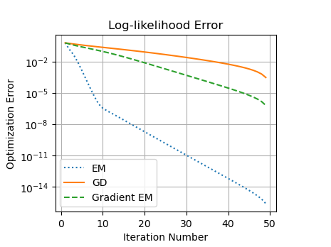
(b)

Figure 1: Convergence of objective errors $\mathcal{L}(\bm{\theta}^{t})-\mathcal{L}(\bm{\theta}^{*})$ and $\mathcal{L}(\bm{\theta}^{t})-\mathcal{L}(\bm{\theta}^{T})$ in Fig 1(a) and Fig 1(b), respectively, averaged over $50$ instances when fitting a SMoLinE.

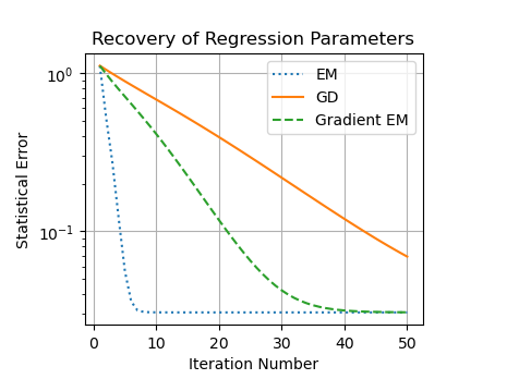
(a)

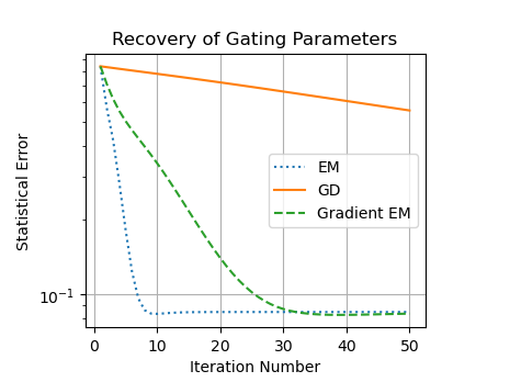
(b)

Figure 2: This figure shows the progress made towards the true parameters, $\frac{\|\bm{\beta}^{t}-\bm{\beta}^{*}\|_{2}}{\|\bm{\beta}^{*}\|_{2}}$ and $\frac{\|\bm{w}^{t}-\bm{w}^{*}\|_{2}}{\|\bm{w}^{*}\|_{2}}$ in figures 2(a) and 2(b) respectively, averaged over $50$ instances when fitting a SMoLinE

Figure 1 shows the objective function progress. EM requires fewer iterations to fit the mixture compared to both Gradient EM and GD, with Gradient EM also outperforming GD in fitting time. Figure 2 illustrates the progress toward recovering the true SMoLinE parameters. Once again, EM requires significantly fewer iterations to fit the mixture compared to both Gradient EM and GD, with Gradient EM also taking considerably less time than GD.

Overall, we observe that all three algorithms exhibit a linear convergence rate, both in optimizing the objective function and fitting the true parameters. This aligns with our theoretical results for MoE and is consistent with findings for Mixtures of Gaussians and Mixtures of Linear Regression in high SNR scenarios.

Validation Experiment on Fashion MNIST. For the small scale proof of concept experiment on Fashion MNIST [XRV17], we alter the dataset so as to simulate a mixture of $2$ Logistic Experts. To do this, we simply perform an inversion transformation on the images at random with probability $\frac{1}{2}$. Effectively, the transformation inverts the images from a white article of clothing on a black background to a black article of clothing on a white background. As can be seen in Table 1, the single expert on the original Fashion MNIST dataset reaches an accuracy of $83.2\%$ on the test set. Meanwhile, the single expert cannot achieve better than an accuracy of $10.2\%$ on the altered dataset. This suggests a $2$-component MoLogE is appropriate for fitting the altered dataset, so long as the ground truth partitioning is linear in image space.

The $2$-component MoLogE to be trained consists of one Linear gating layer of dimension $2\times 28\times 28$, and $2$ logistic experts of dimension $10\times 28\times 28$ each. We randomly initialize each linear layer to be unit norm and execute the algorithms on the same datasets and with the same initializations. For Gradient EM, the only additional code needed over GD is to define the EM Loss function appropriately, and then perform a Gradient Step on the Gating parameters and the Expert parameters separately as describe in Algorithm 1. For EM, for each iteration, we perform several gradient steps in an inner loop to approximately recover the solutions to the sub-problems described in (8). We report our findings in Table 2 and Figure 3.

In Table 2, we report the respective final test accuracy and cross-entropy loss values after $100$ iterations of EM, Gradient EM and GD for fitting a $2$-component MoLogE on the altered Fashion MNIST dataset, averaged over $25$ instances. We see that EM boasts a much improved final test accuracy that nearly recovers the single expert accuracy on the original unaltered Fashion MNIST dataset of $79.2\%$. Meanwhile, Gradient EM also registers an improvement over GD. In Figure 3, we report the progress made on the accuracy and objective function for the test set over the $100$ iterations, averaged over $25$ instances. As was observed in our synthetic experiment, EM takes considerably less iterations to fit the mixture than both Gradient EM and GD, where the former also takes considerably less time to fit the mixture than GD.

Table 1: Performance for single Logistic Expert

	Accuracy	Random Invert
Single Expert	83.2%	No
Single Expert	10.2%	Yes

Table 2: Performance for $2$-Component MoLogE

	Accuracy​	Cross Entropy​
EM	79.2%	0.801
Gradient EM	65.7%	1.30
Gradient Descent​​	61.9%	1.33

(a)

(b)

Figure 3: Test accuracy and objective function, $\frac{1}{n}\sum_{i=1}^{n}\mathbbm{1}_{\hat{y_{i}}=y_{i}}$ and $\mathcal{L}(\bm{\theta}^{t})$ in 3(a) and 3(b), respectively, averaged over $25$ instances for a $2$-component MoLogE.

7 Conclusion

In this paper, we addressed the problem of Mixtures of Experts (MoE), focusing on the use of the EM method to solve these problems. We first showed that the EM update for MoE could be interpreted as a Mirror Descent step on the log-likelihood with a unit step size and a KL divergence regularizer, extending the result of [KKS22] beyond the exponential family. Building on this, we characterized different convergence rates for EM in this setting under various assumptions about the log-likelihood function and specified when these assumptions held. We also compared EM with gradient descent empirically and showed that EM outperformed gradient descent in both convergence rate and final performance.

Appendix A EM is Mirror Descent for SMoLogE and SMoLinE

In this section, we provide the full and detailed proof of the main result, Theorem 4.1. For ease of comprehension and in the hope that this will provide useful insights into other types of non-exponential family mixtures for which EM is also connected to MD, we prove our result following the same general ideas as that of [KKS22, Proposition 1]. We split the proof into two parts (SMoLinE and SMoLogE) which can be found in Appendix A.1 and A.2.

For ease of reading, we re-state the theorem below:
Theorem 4.1: For SMoLinE and SMoLogE, there is a mirror map $A(\bm{\theta})$ such that the EM update in (8) simplifies and is equivalent to

$$\operatorname*{arg\,min}_{\bm{\theta}\in\Omega}\langle\mathcal{\nabla L(\bm{\theta})},\bm{\theta}-\bm{\theta}^{t}\rangle+D_{A}(\bm{\theta},\bm{\theta}^{t}),$$

where $\forall\bm{\phi},\bm{\theta}\in\Omega$ the divergence function $D_{A}(\bm{\theta},\bm{\theta}^{t})$ is equal to the $KL$ divergence on the complete data:

$$D_{A}(\bm{\phi},\bm{\theta})=\text{KL}[p(\bm{x},y,z;\bm{\theta})\|p(\bm{x},y,z;\bm{\phi})].$$

In particular, in the case of SMoLinE,

$$A(\bm{\theta})=\mathbb{E}_{\bm{X}}\left[\frac{(\bm{x}^{\top}\bm{\beta})^{2}}{2}+\log\left(1+e^{\bm{x}^{\top}\bm{w}}\right)\right],$$

while in the case of SMoLogE,

$$A(\bm{\theta})=\mathbb{E}_{\bm{X}}\left[\log\left(\left(1+e^{\bm{x}^{\top}\bm{\beta}}\right)\left(1+e^{\bm{x}^{\top}\bm{w}}\right)\right)\right].$$

Finally, in both cases, the map $A(\bm{\theta})$ is strictly convex in $\bm{\theta}$ and $\mathcal{L}(\bm{\theta})$ is $1$-smooth relative to $A(\bm{\theta})$.

A.1 Proof of Theorem 4.1 for SMoLinE

Proof.

Recall that we consider a $2$ component SMoLinE (see Section 3.1) where $z\in\{-1,1\}$ is the latent unobserved variable, and

• $\bm{x}\sim\mathcal{N}(\bm{0},\bm{I}_{d})$,

• $P(z|\bm{x};\bm{w})=\frac{\exp\{\frac{z+1}{2}\bm{x}^{\top}{\bm{w}}\}}{1+e^{\bm{x}^{\top}{\bm{w}}}}$,

• $p(y|\bm{x},z;\bm{\beta})=\frac{\exp\left\{-\frac{(y-z\bm{x}^{\top}\bm{\beta})^{2}}{2}\right\}}{\sqrt{2\pi}}$.

We begin by deriving a near exponential form of the complete data probability density function $p(\bm{x},z,y;\bm{\theta})$:

$$p(\bm{x},y,z;\bm{\theta})$$

$$=p(y|\bm{x},z;\bm{\theta})P(z|\bm{x};\bm{\theta})p(\bm{x})$$

$$=\exp\{\log p(y|\bm{x},z;\bm{\beta})+\log P(z|\bm{x};\bm{w})+\log p(\bm{x})\}$$

$$=\exp\left\{\frac{-(y-z\bm{x}^{\top}\bm{\beta})^{2}}{2}-\frac{1}{2}\log(2\pi)+\left(\frac{z+1}{2}\right)\bm{x}^{\top}\bm{w}-\log(1+e^{\bm{x}^{\top}\bm{w}})+\log p(\bm{x})\right\}$$

$$=\exp\left\{\frac{-y^{2}}{2}+yz\bm{x}^{\top}\bm{\beta}-\frac{z^{2}(\bm{x}^{\top}\bm{\beta})^{2}}{2}+\left(\frac{z+1}{2}\right)\bm{x}^{\top}\bm{w}-\log(1+e^{\bm{x}^{\top}\bm{w}})+\log p(\bm{x})-\frac{1}{2}\log(2\pi)\right\}$$

$$=\exp\left\{\left\langle\begin{bmatrix}yz\bm{x}\\ \frac{z\bm{x}}{2}\end{bmatrix},\begin{bmatrix}\bm{\beta}\\ \bm{w}\end{bmatrix}\right\rangle+\frac{\bm{x}^{\top}\bm{w}}{2}-\frac{(\bm{x}^{\top}\bm{\beta})^{2}}{2}-\log(1+e^{\bm{x}^{\top}\bm{w}})+\log p(\bm{x})-\frac{y^{2}}{2}-\frac{1}{2}\log(2\pi)\right\}.$$

Thus we have recovered the decomposition,

$$p(\bm{x},y,z;\bm{\theta})=\exp\left\{\left\langle\underbrace{\begin{bmatrix}\frac{z\bm{x}}{2}\\ yz\bm{x}\end{bmatrix}}_{S(\bm{x},y,z)},\begin{bmatrix}\bm{w}\\ \bm{\beta}\end{bmatrix}\right\rangle+a(\bm{x},y,\bm{\theta})\right\},$$ (30)

where in $a(\bm{x},y,\bm{\theta})$, the feature variable $\bm{x}$ cannot be linearly separated from the parameter $\bm{\theta}$:

$$a(\bm{x},y,\bm{\theta})=\frac{\bm{x}^{\top}\bm{w}}{2}-\frac{(\bm{x}^{\top}\bm{\beta})^{2}}{2}-\log\left(1+e^{\bm{x}^{\top}\bm{w}}\right)+\log p(\bm{x})-\frac{y^{2}}{2}-\frac{1}{2}\log(2\pi).$$

At this point, we pause and discuss the implications of the obtained form. First we recall that for a random variable $\bm{U}$ to belong to an exponential family, it must satisfy

$$p(\bm{u};\bm{\theta})=h(\bm{u})\exp\left\{{\langle s(\bm{u}),\bm{\theta}\rangle-A(\bm{\theta})}\right\}$$

for some $h(\cdot),s(\cdot),\bm{\theta},A(\cdot)$ that are called the normalization function, sufficient statistics, natural parameters, and log-partition function respectively. To clarify, we note that 1) $A(\bm{\theta})$ must be a function of the parameters only and cannot depend on $\bm{u}$ and 2) $h(\bm{u})$ must be a function of the variable $\bm{u}$ only and cannot depend on the parameters. In other words, it must be that $h(\bm{u})$ and $A(\bm{\theta})$ are linearly separated inside the $\exp$. With the above in mind, we see that SMoLinE is not an exponential family. Further, we remark that the above formulation showing $S(\bm{x},y,z)$ is linear with $(\bm{w},\bm{\beta})^{\top}$ does not extend beyond the symmetric setting of the Mixture of Linear Experts; for $k\geq 3$, this relationships becomes non-linear. This turns out to be problematic for showing EM is equivalent to MD for $k\geq 3$. Lastly, note that taking the expectation of $a(\bm{x},y,\bm{\theta})$ over $(\bm{x},y)\sim p(\bm{x},y;\bm{\theta}^{*})$ yields,

$$\mathbb{E}_{\bm{X},Y}[a(\bm{x},y,\bm{\theta})] =-\mathbb{E}_{\bm{X}}\left[\frac{(\bm{x}^{\top}\bm{\beta})^{2}}{2}+\log\left(1+e^{\bm{x}^{\top}\bm{w}}\right)\right]-C$$

$$=-A(\bm{\theta})-C,$$

where the above follows from $\mathbb{E}_{\bm{X}}[\frac{\bm{x}^{\top}\bm{w}}{2}]=0$ and $C:=-\mathbb{E}_{\bm{X},Y}[\log p(\bm{x})-\frac{y^{2}}{2}-\frac{1}{2}\log(2\pi)]$ is not a function of the parameter $\bm{\theta}$. With the obtained form (30), we now continue with the proof.

Part a): Show EM is MD, i.e., $\operatorname*{arg\,min}_{\bm{\theta}\in\Omega}Q(\bm{\theta}|\bm{\theta}^{t})=\operatorname*{arg\,min}_{\bm{\theta}\in\Omega}\langle\mathcal{\nabla L(\bm{\theta})},\bm{\theta}-\bm{\theta}^{t}\rangle+D_{A}(\bm{\theta},\bm{\theta}^{t})$.

Taking the appropriate expectation, the EM objective $Q$ can be written as

$$Q(\bm{\theta}|\bm{\theta}^{t}) =-\mathbb{E}_{\bm{X},Y}\left[\mathbb{E}_{Z|\bm{x},y;\bm{\theta}^{t}}\left[\log p(\bm{x},y,z;\bm{\theta})\right]\right]$$

$$=-\mathbb{E}_{\bm{X},Y}\left[\mathbb{E}_{Z|\bm{x},y;\bm{\theta}^{t}}\left[\langle S(\bm{x},y,z),\bm{\theta}\rangle+a(\bm{x},y,\bm{\theta})\right]\right]$$

$$=-\mathbb{E}_{\bm{X},Y}\left[a(\bm{x},y,\bm{\theta})\right]-\mathbb{E}_{\bm{X},Y}\left[\mathbb{E}_{Z|\bm{x},y;\bm{\theta}^{t}}\left[\langle S(\bm{x},y,z),\bm{\theta}\rangle\right]\right]$$

$$=A(\bm{\theta})-\left\langle s(\bm{\theta}^{t}),\bm{\theta}\right\rangle+C$$

where $s(\bm{\theta}^{t}):=\mathbb{E}_{\bm{X},Y}\mathbb{E}_{Z|\bm{x},y;\bm{\theta}^{t}}[S(\bm{x},y,z)]$. As a consequence, it is also true that

$$\nabla Q(\bm{\theta}^{t}|\bm{\theta}^{t})=\nabla A(\bm{\theta}^{t})-s(\bm{\theta}^{t}).$$ (31)

Continuing, we use the above to simplify the expression for $Q(\bm{\theta}|\bm{\theta}^{t})-Q(\bm{\theta}^{t}|\bm{\theta}^{t})$ that will subsequently give us the MD loss:

$$Q(\bm{\theta}|\bm{\theta}^{t})-Q(\bm{\theta}^{t}|\bm{\theta}^{t}) =A(\bm{\theta})-\left\langle s(\bm{\theta}^{t}),\bm{\theta}\right\rangle-A(\bm{\theta}^{t})+\left\langle s(\bm{\theta}^{t}),\bm{\theta}^{t}\right\rangle$$

$$=-\left\langle s(\bm{\theta}^{t}),\bm{\theta}-\bm{\theta}^{t}\right\rangle+\langle\nabla A(\bm{\theta}^{t}),\bm{\theta}-\bm{\theta}^{t}\rangle-\langle\nabla A(\bm{\theta}^{t}),\bm{\theta}-\bm{\theta}^{t}\rangle+A(\bm{\theta})-A(\bm{\theta}^{t})$$

$$\stackrel{{\scriptstyle i)}}{{=}}\left\langle\nabla Q(\bm{\theta}^{t}|\bm{\theta}^{t}),\bm{\theta}-\bm{\theta}^{t}\right\rangle+D_{A}(\bm{\theta},\bm{\theta}^{t})$$

$$\stackrel{{\scriptstyle ii)}}{{=}}\left\langle\nabla\mathcal{L}(\bm{\theta}^{t}),\bm{\theta}-\bm{\theta}^{t}\right\rangle+D_{A}(\bm{\theta},\bm{\theta}^{t})$$

where we first adding and subtracting $\langle\nabla A(\bm{\theta}^{t}),\bm{\theta}-\bm{\theta}^{t}\rangle$ then $i)$ follows from (31) and $ii)$ follows from $\nabla\mathcal{L}(\bm{\theta})=\nabla Q(\bm{\theta}|\bm{\theta})$ (see Section 3 for the derivation).

Finally, the first part of our result follows trivially as

$$\operatorname*{arg\,min}_{\bm{\theta}\in\Omega}Q(\bm{\theta}|\bm{\theta}^{t})=\operatorname*{arg\,min}_{\bm{\theta}\in\Omega}Q(\bm{\theta}|\bm{\theta}^{t})-Q(\bm{\theta}^{t}|\bm{\theta}^{t}).$$

Part b): Show $D_{A}(\bm{\phi},\bm{\theta})=\text{KL}[p(\bm{x},y,z;\bm{\theta})\|p(\bm{x},y,z;\bm{\phi})]$

This result follows simply from decomposing $\text{KL}[p(\bm{x},y,z;\bm{\theta})\|p(\bm{x},y,z;\bm{\phi})]$ as follows:

$$\text{KL}[p(\bm{x},y,z;\bm{\theta})\|p(\bm{x},y,z;\bm{\phi})]=\mathbb{E}_{\bm{X},Y,Z|\bm{\theta}}\left[\log\frac{p(\bm{x},y,z;\bm{\theta})}{p(\bm{x},y,z;\bm{\phi})}\right]$$

$$\stackrel{{\scriptstyle\eqref{eqn: Not Exp SMOLINE}}}{{=}}\langle s(\bm{\theta}),\bm{\theta}-\bm{\phi}\rangle-A(\bm{\theta})+A(\phi)\pm\mathbb{E}_{\bm{X},Y|\bm{\theta}}\left[\log p(\bm{x})-\frac{y^{2}}{2}-\frac{1}{2}\log(2\pi)\right]$$

$$=A(\bm{\phi})-A(\bm{\theta})-\langle s(\bm{\theta}),\bm{\phi}-\bm{\theta}\rangle$$

$$\stackrel{{\scriptstyle i)}}{{=}}A(\bm{\phi})-A(\bm{\theta})-\langle\nabla A(\bm{\theta}),\bm{\phi}-\bm{\theta}\rangle.$$

where $i)$ follows from the fact that $\bm{\phi}=\bm{\theta}$ minimizes $-\mathbb{E}_{\bm{X},Z,Y|\bm{\theta}}\left[\log p(\bm{x},y,z;\bm{\phi})\right]$. To see this, we use Jensen’s inequality:

$$0 \leq-\mathbb{E}_{\bm{X},Z,Y|\bm{\theta}}\left[\log p(\bm{x},y,z;\bm{\theta})\right]$$

$$\stackrel{{\scriptstyle\text{Jensen's}}}{{\leq}}-\log\mathbb{E}_{\bm{X},Z,Y|\bm{\theta}}\left[p(\bm{x},y,z;\bm{\theta})\right]=-\log\int_{\bm{x},y,z}p(\bm{x},y,z:\bm{\theta})^{2}d\bm{x}dzdy$$

$$\stackrel{{\scriptstyle\text{Jensen's}}}{{\leq}}-\log\left(\int_{\bm{x},y,z}p(\bm{x},y,z;\bm{\theta})d\bm{x}dzdy\right)^{2}=-\log(1)=0.$$

Finally, taking the derivative with respect to $\phi$ and setting equal to $0$ completes the proof:

$$\bm{0} =\frac{\partial}{\partial\bm{\theta}}\mathbb{E}_{\bm{X},Z,Y|\bm{\theta}}\left[\log p(\bm{x},y,z;\bm{\phi})\right]|_{\bm{\phi}=\bm{\theta}}$$

$$=\mathbb{E}_{\bm{X},Z,Y|\bm{\theta}}\left[S(\bm{x},y,z)+\frac{\partial}{\partial\bm{\phi}}a(\bm{x},y,\bm{\phi})|_{\bm{\phi}=\bm{\theta}}\right]$$

$$=s(\bm{\theta})-\nabla A(\bm{\theta}).$$

Part c): Show $\mathcal{L}(\bm{\theta})$ is $1$-smooth relative to $A(\bm{\theta})$.
The function $\mathcal{L}(\bm{\theta})$ is said to be $1$-smooth relative to $A(\bm{\theta})$ if for all $\bm{\phi},\bm{\theta}$, it holds that

$$\mathcal{L}(\bm{\theta})\leq\mathcal{L}(\bm{\phi})+\left\langle\nabla\mathcal{L}(\bm{\phi},\bm{\theta}-\bm{\phi}\right\rangle+D_{A}(\bm{\theta},\bm{\phi}).$$

Recall the following from Section 3. The objective function $\mathcal{L}(\bm{\theta})$ is related to the EM objective $Q(\bm{\phi}|\bm{\theta})$ by (9),

$$\mathcal{L}(\bm{\theta})=Q(\bm{\theta}|\bm{\phi})-H(\bm{\theta}|\bm{\phi}),$$

where $H(\bm{\phi}|\bm{\theta})\geq 0$ and $H(\bm{\theta}|\bm{\theta})=0$ for all $\bm{\phi},\bm{\theta}\in\Omega$. Consequently, it then holds that for all $\bm{\phi},\bm{\theta}\in\Omega$,

$$\mathcal{L}(\bm{\theta}) =Q(\bm{\theta}|\bm{\theta})$$ (32)

$$\mathcal{L}(\bm{\theta}) \leq Q(\bm{\theta}|\bm{\phi}).$$ (33)

Recall also from part a) that $Q(\bm{\theta}|\bm{\phi})-Q(\bm{\phi}|\bm{\phi})=\left\langle\nabla\mathcal{L}(\bm{\phi}),\bm{\theta}-\bm{\phi}\right\rangle+D_{A}(\bm{\theta},\bm{\phi})$. Then, the claim follows naturally from the above as follows:

$$\mathcal{L}(\bm{\theta}) \stackrel{{\scriptstyle\eqref{eqn: Q is upper bound}}}{{\leq}}Q(\bm{\theta}|\bm{\phi})$$

$$\stackrel{{\scriptstyle a)}}{{=}}Q(\bm{\phi}|\bm{\phi})+\left\langle\nabla\mathcal{L}(\bm{\phi}),\bm{\theta}-\bm{\phi}\right\rangle+D_{A}(\bm{\theta},\bm{\phi})$$

$$\stackrel{{\scriptstyle\eqref{eqn: Q equality to L}}}{{=}}\mathcal{L}(\bm{\phi})+\left\langle\nabla\mathcal{L}(\bm{\phi}),\bm{\theta}-\bm{\phi}\right\rangle+D_{A}(\bm{\theta},\bm{\phi})$$

It follows that $\mathcal{L}(\bm{\theta})$ is $1$-smooth relative to $A(\bm{\theta})$.

Part d): $A(\bm{\theta})$ and the MD objective is convex with respect to $\bm{\theta}$.
Here, we will show that the mirror descent objective is strongly convex in $\bm{\theta}$. It is important for this to hold so that the iterations of MD are well-defined; the minimizer of a strongly convex objective exists and is unique.

Note that the mirror descent objective, $\langle\mathcal{\nabla L(\bm{\theta})},\bm{\theta}-\bm{\theta}^{t}\rangle+D_{A}(\bm{\theta},\bm{\theta}^{t})$, is strongly convex in $\bm{\theta}$ if $A(\bm{\theta})$ is strongly convex in $\bm{\theta}$. Therefore, since $A(\bm{\theta})$ given in (17) is twice continuously differentiable, it is strongly convex with respect to $\bm{\theta}$ if and only if $\nabla^{2}A(\bm{\theta})\succeq r\bm{I}_{2d}$, for some $r>0$. We begin:

$$\nabla^{2}A(\bm{\theta}) =\frac{\partial^{2}}{\partial\bm{\theta}^{2}}\mathbb{E}_{\bm{X}}\left[\frac{(\bm{x}^{\top}\bm{\beta})^{2}}{2}+\log\left(1+e^{\bm{x}^{\top}\bm{w}}\right)\right]$$

$$=\mathbb{E}_{\bm{X}}\left[\frac{\partial^{2}}{\partial\bm{\theta}^{2}}\left(\frac{(\bm{x}^{\top}\bm{\beta})^{2}}{2}+\log\left(1+e^{\bm{x}^{\top}\bm{w}}\right)\right)\right]$$

$$=\begin{pmatrix}\mathbb{E}_{\bm{X}}\left[\bm{x}\bm{x}^{\top}\frac{e^{\bm{x}^{\top}\bm{w}}}{\left(1+e^{\bm{x}^{\top}\bm{w}}\right)^{2}}\right]&\bm{0}\\ \bm{0}&\mathbb{E}_{\bm{X}}\left[\bm{x}\bm{x}^{\top}\right]\end{pmatrix}$$

$$=\begin{pmatrix}\mathbb{E}_{\bm{X}}\left[\bm{x}\bm{x}^{\top}\frac{e^{\bm{x}^{\top}\bm{w}}}{\left(1+e^{\bm{x}^{\top}\bm{w}}\right)^{2}}\right]&\bm{0}\\ \bm{0}&\bm{I}_{d}\end{pmatrix}$$

where the last line follows from the assumption that $\bm{x}$ is sampled from a unit spherical Gaussian distribution: $\mathbb{E}_{\bm{X}}\left[\bm{x}\bm{x}^{\top}\right]=\bm{I}_{d}$ for $\bm{x}\sim\mathcal{N}(\bm{0},\bm{I}_{d})$.

From the above, we see that $A(\bm{\theta})$ is strictly convex, and it is strongly convex if $\mathbb{E}_{\bm{X}}\left[\bm{x}\bm{x}^{\top}\frac{e^{\bm{x}^{\top}\bm{w}}}{\left(1+e^{\bm{x}^{\top}\bm{w}}\right)^{2}}\right]\succeq r\bm{I}_{d}$ for some $r>0$. This follows from Lemma B.2 where we show its eigenvalues are bounded below by $\min\left\{\Omega\left(\frac{1}{\|\bm{w}\|_{2}}\right),\Omega\left(\frac{1}{\|\bm{w}\|_{2}^{3}}\right)\right\}$. Thus, it holds that

$$\nabla^{2}A(\bm{\theta})\succeq\min\left\{\Omega\left(\frac{1}{\|\bm{w}\|_{2}}\right),\Omega\left(\frac{1}{\|\bm{w}\|_{2}^{3}}\right),1\right\}\bm{I}_{2d}.$$

Restricting the feasible set $\Omega$ to be all $\bm{\theta}\in\mathbb{R}^{2d}$ with $\|\bm{\theta}\|_{2}\leq N$ for some $N\in[0,\infty)$, it holds that $A(\bm{\theta})$ is strongly convex with respect to $\bm{\theta}$ on $\Omega$.

With part d) proven, this concludes the proof of Theorem 4.1 for SMoLinE. We now prove the same for SMoLogE, referring to this section where necessary.

∎

A.2 Proof of Theorem 4.1 for SMoLogE

Proof.

Recall that we consider a $2$ component SMoLogE (see Section 3.1) where $z\in\{-1,1\}$ is the latent unobserved variable, and

• $\bm{x}\sim\mathcal{N}(\bm{0},\bm{I}_{d})$,

• $P(z|\bm{x};\bm{w})=\frac{\exp\{\frac{z+1}{2}\bm{x}^{\top}{\bm{w}}\}}{1+e^{\bm{x}^{\top}{\bm{w}}}}.$

• $P(y|\bm{x},z;\bm{\beta})=\frac{\exp\{\bm{\left missing}(\frac{yz+1}{2}\right)x^{\top}\bm{\beta}\}}{1+e^{\bm{x}^{\top}\bm{\beta}}}$.

We begin by deriving a near exponential form of the complete data probability density function $p(\bm{x},z,y;\bm{\theta})$:

$$p(\bm{x},z,y;\bm{\theta})$$

$$=P(y|\bm{x},z;\bm{\theta})P(z|\bm{x};\bm{\theta})p(\bm{x})$$

$$=\exp\{\log P(y|\bm{x},z;\bm{\beta})+\log P(z|\bm{x};\bm{w})+\log p(\bm{x})\}$$

$$=\exp\left\{\log\left(\left(\frac{\exp\{\bm{x}^{\top}\bm{\beta}\}}{1+e^{\bm{x}^{\top}\bm{\beta}}}\right)^{\frac{yz+1}{2}}\left(\frac{1}{1+e^{\bm{x}^{\top}\bm{\beta}}}\right)^{1-\frac{yz+1}{2}}\right)+\left(\frac{z+1}{2}\right)\bm{x}^{\top}\bm{w}-\log(1+e^{\bm{x}^{\top}\bm{w}})+\log p(\bm{x})\right\}$$

$$=\exp\left\{{\frac{yz+1}{2}}\log\left(\frac{\exp\{\bm{x}^{\top}\bm{\beta}\}}{1+e^{\bm{x}^{\top}\bm{\beta}}}\right)+\left(1-\frac{yz+1}{2}\right)\log\left(\frac{1}{1+e^{\bm{x}^{\top}\bm{\beta}}}\right)+\left(\frac{z+1}{2}\right)\bm{x}^{\top}\bm{w}-\log(1+e^{\bm{x}^{\top}\bm{w}})+\log p(\bm{x})\right\}$$

$$=\exp\left\{\left(\frac{yz+1}{2}\right)\bm{x}^{\top}\bm{\beta}-\log\left(1+e^{\bm{x}^{\top}\bm{\beta}}\right)+\left(\frac{z+1}{2}\right)\bm{x}^{\top}\bm{w}-\log(1+e^{\bm{x}^{\top}\bm{w}})+\log p(\bm{x})\right\}$$

$$=\exp\left\{\left\langle\begin{bmatrix}\frac{yz\bm{x}}{2}\\ \frac{z\bm{x}}{2}\end{bmatrix},\begin{bmatrix}\beta\\ w\end{bmatrix}\right\rangle+\frac{\bm{x}^{\top}(\bm{w}+\bm{\beta})}{2}-\log\left[\left(1+e^{\bm{x}^{\top}\bm{\beta}}\right)\left(1+e^{\bm{x}^{\top}\bm{w}}\right)\right]+\log p(\bm{x})\right\}.$$

Thus we have recovered the decomposition,

$$p(\bm{x},y,z;\bm{\theta})=\exp\left\{\left\langle\begin{bmatrix}\frac{yz\bm{x}}{2}\\ \frac{z\bm{x}}{2}\end{bmatrix},\begin{bmatrix}\bm{\beta}\\ \bm{w}\end{bmatrix}\right\rangle+a(\bm{x},y,\bm{\theta})\right\},,$$ (34)

where in $a(\bm{x},y,\bm{\theta})$, $\bm{x}$ cannot be linearly separated from the parameter $\bm{\theta}$:

$$a(\bm{x},y,\bm{\theta})=\frac{\bm{x}^{\top}(\bm{w}+\bm{\beta})}{2}-\log\left[\left(1+e^{\bm{x}^{\top}\bm{\beta}}\right)\left(1+e^{\bm{x}^{\top}\bm{w}}\right)\right]+\log p(\bm{x}).$$

Similar to SMoLinE, we can see that $p(\bm{x},y,z;\bm{\theta})$ does not belong to an exponential family of distribution. Also, note that taking the expectation of $a(\bm{x},y,\bm{\theta})$ over $(\bm{x},y)\sim p(\bm{x},y;\bm{\theta}^{*})$ yields,

$$\mathbb{E}_{\bm{X},Y}[a(\bm{x},y,\bm{\theta})] =-\mathbb{E}_{\bm{X}}\left[\log\left[\left(1+e^{\bm{x}^{\top}\bm{\beta}}\right)\left(1+e^{\bm{x}^{\top}\bm{w}}\right)\right]\right]-C$$

$$=-A(\bm{\theta})-C,$$

where the above follows from $\mathbb{E}_{\bm{X}}[\frac{\bm{x}^{\top}(\bm{w}+\bm{\beta})}{2}]=0$ and $C:=-\mathbb{E}_{\bm{X},Y|\bm{\theta}^{*}}[\log p(\bm{x})]$ is not a function of the parameter $\bm{\theta}$. We now continue with the proof.

From here on, the proofs of part a), part b) and part c) follow identically from that of SMoLinE, so we will refer to Appendix A.1 for those proofs. We will now show part d).

Part d):$A(\bm{\theta})$ and the MD objective is convex with respect to $\bm{\theta}$.
Here, we will show that the mirror descent objective is strongly convex in $\bm{\theta}$. It is important for this to hold so that the iterations of MD are well-defined; the minimizer of a strongly convex objective exists and is unique.

Note that the mirror descent objective, $\langle\mathcal{\nabla L(\bm{\theta})},\bm{\theta}-\bm{\theta}^{t}\rangle+D_{A}(\bm{\theta},\bm{\theta}^{t})$, is strongly convex in $\bm{\theta}$ if $A(\bm{\theta})$ is strongly convex in $\bm{\theta}$. Therefore, since $A(\bm{\theta})$ given in (17) is twice continuously differentiable, it is strongly convex with respect to $\bm{\theta}$ if and only if $\nabla^{2}A(\bm{\theta})\succeq r\bm{I}_{2d}$, for some $r>0$. We begin:

$$\nabla^{2}A(\bm{\theta}) =\frac{\partial^{2}}{\partial\bm{\theta}^{2}}\mathbb{E}_{\bm{X}}\left[\log\left(\left(1+e^{\bm{x}^{\top}\bm{\beta}}\right)\left(1+e^{\bm{x}^{\top}\bm{w}}\right)\right)\right]$$

$$=\mathbb{E}_{\bm{X}}\left[\frac{\partial^{2}}{\partial\bm{\theta}^{2}}\left(\log\left(1+e^{\bm{x}^{\top}\bm{\beta}}\right)+\log\left(1+e^{\bm{x}^{\top}\bm{w}}\right)\right)\right]$$

$$=\begin{pmatrix}\mathbb{E}_{\bm{X}}\left[\bm{x}\bm{x}^{\top}\frac{e^{\bm{x}^{\top}\bm{w}}}{\left(1+e^{\bm{x}^{\top}\bm{w}}\right)^{2}}\right]&\bm{0}\\ \bm{0}&\mathbb{E}_{\bm{X}}\left[\bm{x}\bm{x}^{\top}\frac{e^{\bm{x}^{\top}\bm{\beta}}}{\left(1+e^{\bm{x}^{\top}\bm{\beta}}\right)^{2}}\right]\end{pmatrix}$$

$$=\begin{pmatrix}\mathbb{E}_{\bm{X}}\left[\bm{x}\bm{x}^{\top}\frac{e^{\bm{x}^{\top}\bm{w}}}{\left(1+e^{\bm{x}^{\top}\bm{w}}\right)^{2}}\right]&\bm{0}\\ \bm{0}&\mathbb{E}_{\bm{X}}\left[\bm{x}\bm{x}^{\top}\frac{e^{\bm{x}^{\top}\bm{\beta}}}{\left(1+e^{\bm{x}^{\top}\bm{\beta}}\right)^{2}}\right]\end{pmatrix}.$$

From the above, we see that $A(\bm{\theta})$ is strictly convex, and it is strongly convex if $\mathbb{E}_{\bm{X}}\left[\bm{x}\bm{x}^{\top}\frac{e^{\bm{x}^{\top}\bm{w}}}{\left(1+e^{\bm{x}^{\top}\bm{w}}\right)^{2}}\right]\succeq r\bm{I}_{d}$ and $\mathbb{E}_{\bm{X}}\left[\bm{x}\bm{x}^{\top}\frac{e^{\bm{x}^{\top}\bm{\beta}}}{\left(1+e^{\bm{x}^{\top}\bm{\beta}}\right)^{2}}\right]\succeq r\bm{I}_{d}$ for some $r>0$. This follows from Lemma B.2 where we show their respective eigenvalues are bounded below by, $\min\left\{\Omega\left(\frac{1}{\|\bm{w}\|_{2}}\right),\Omega\left(\frac{1}{\|\bm{w}\|_{2}^{3}}\right)\right\}$ and $\min\left\{\Omega\left(\frac{1}{\|\bm{\beta}\|_{2}}\right),\Omega\left(\frac{1}{\|\bm{\beta}\|_{2}^{3}}\right)\right\}$. Thus, it holds that

$$\nabla^{2}A(\bm{\theta})\succeq\min\left\{\Omega\left(\frac{1}{\|\bm{w}\|_{2}}\right),\Omega\left(\frac{1}{\|\bm{w}\|_{2}^{3}}\right),\Omega\left(\frac{1}{\|\bm{\beta}\|_{2}}\right),\Omega\left(\frac{1}{\|\bm{\beta}\|_{2}^{3}}\right)\right\}\bm{I}_{2d}.$$

Restricting $\Omega$ to be all $\bm{\theta}$ with $\|\bm{\theta}\|_{2}\leq N$ for some $N\in[0,\infty)$, it holds that $A(\bm{\theta})$ is strongly convex with respect to $\bm{\theta}$ on $\Omega$.

With part d) proven, this concludes the proof of Theorem 4.1 for SMoLinE. We now prove the same for SMoLogE, referring to this section where necessary.

∎

Appendix B Convergence Analysis

In this section, we provide the proofs of Corollary 5.1, Theorem 5.2 and Theorem 5.3. As well, in the last subsection, we discuss the consequences of these results.

B.1 Convergence Properties of Mirror Descent: Corollary 5.1

In this section, we provide a contextual proof for Corollary 5.1 which follows trivially from previous work on MD (see [KKS22, Proposition 2, Corollary 1, and Corollary 3] and [LFN17, Theorem 3.1] for a comprehensive overview of the many convergence properties of MD). The proof is divided into three parts that correspond to each of the three sub-results of the corollary.

For ease of reading, we re-state the Corollary below:
Corollary 5.1: For SMoLinE, SMoLogE with mirror map $A(\bm{\theta})$ given as (17) (18) respectively, and denoting $D_{A}(\bm{\theta}^{t},\bm{\theta}^{t+1})\!:=\!\text{KL}[p(\bm{x},y,z;\bm{\theta}^{t+1})\|p(\bm{x},y,z;\bm{\theta}^{t})]$, the EM iterates $\{\bm{\theta}^{t}\}_{t\in[T]}$ satisfy:

• Stationarity. For no additional conditions,

  $$\min_{t\in[T]}D_{A}(\bm{\theta}^{t+1},\bm{\theta}^{t})\leq\frac{\mathcal{L}(\bm{\theta}^{1})-\mathcal{L}(\bm{\theta}^{*})}{T};$$ (35)

• Sub-linear Rate to $\bm{\theta}^{*}$. If $\bm{\theta}^{1}$ is initialized in $\Theta$, a locally convex region of $\mathcal{L}(\bm{\theta})$ containing $\bm{\theta}^{*}$, then

  $$\mathcal{L}(\bm{\theta}^{T})-\mathcal{L}(\bm{\theta}^{*})\leq\frac{D_{A}(\bm{\theta}^{*},\bm{\theta}^{1})}{T}$$ (36)

• Linear Rate to $\bm{\theta}^{*}$. If $\bm{\theta}^{1}$ is initialized in $\Theta\subseteq\Omega$, a locally strongly convex region of $\mathcal{L}(\bm{\theta})$ relative to $A(\bm{\theta})$ that contains $\bm{\theta}^{*}$, then

  $$\mathcal{L}(\bm{\theta}^{T})-\mathcal{L}(\bm{\theta}^{*})\leq(1-\alpha)^{T}(\mathcal{L}(\bm{\theta}^{1})-\mathcal{L}(\bm{\theta}^{*})).$$ (37)

Proof.

The proof is divided into three parts that correspond to each of the three sub-results of the corollary.

Part 1): Stationarity.
Given Theorem 4.1, this proof follows from identical arguments to that of [KKS22, Proposition 2]. We write it below for completeness.

Recall from Theorem 4.1 that $\bm{\theta}^{t+1}$ is obtained as the minimizer of the convex objective, (14):

$$\langle\nabla\mathcal{L}(\bm{\theta}^{t}),\bm{\theta}-\bm{\theta}^{t}\rangle+D_{A}(\bm{\theta},\bm{\theta}^{t}).$$

As such, differentiating and setting equal to $0$, it holds that $\bm{\theta}^{t+1}$ satisfies

$$\nabla\mathcal{L}(\bm{\theta}^{t})=\nabla A(\bm{\theta}^{t})-\nabla A(\bm{\theta}^{t+1})$$ (38)

Further, by the above together with relative smoothness, it holds that

$$\mathcal{L}(\bm{\theta}^{t+1}) \leq\mathcal{L}(\bm{\theta}^{t})+\langle\nabla\mathcal{L}(\bm{\theta}^{t}),\bm{\theta}^{t+1}-\bm{\theta}^{t}\rangle+D_{A}(\bm{\theta}^{t+1},\bm{\theta}^{t})$$

$$=\mathcal{L}(\bm{\theta}^{t})+\langle\nabla A(\bm{\theta}^{t})-\nabla A(\bm{\theta}^{t+1}),\bm{\theta}^{t+1}-\bm{\theta}^{t}\rangle+D_{A}(\bm{\theta}^{t+1},\bm{\theta}^{t})$$

$$=\mathcal{L}(\bm{\theta}^{t})-\langle\nabla A(\bm{\theta}^{t+1}),\bm{\theta}^{t+1}-\bm{\theta}^{t}\rangle+A(\bm{\theta}^{t+1})-A(\bm{\theta}^{t})$$

$$=\mathcal{L}(\bm{\theta}^{t})-D_{A}(\bm{\theta}^{t},\bm{\theta}^{t+1}).$$

Thus it we have shown that

$$D_{A}(\bm{\theta}^{t},\bm{\theta}^{t+1})\leq\mathcal{L}(\bm{\theta}^{t})-\mathcal{L}(\bm{\theta}^{t+1}).$$ (39)

The claim then follows from taking the mean over $T$ iterations:

$$\min_{t\leq T}D_{A}(\bm{\theta}^{t},\bm{\theta}^{t+1})\leq\frac{1}{T}\sum_{t=1}^{T}D_{A}(\bm{\theta}^{t},\bm{\theta}^{t+1})\leq\frac{1}{T}\sum_{t=1}^{T}\mathcal{L}(\bm{\theta}^{t})-\mathcal{L}(\bm{\theta}^{t+1})=\frac{\mathcal{L}(\bm{\theta}^{1})-\mathcal{L}(\bm{\theta}^{T})}{T}\leq\frac{\mathcal{L}(\bm{\theta}^{1})-\mathcal{L}(\bm{\theta}^{*})}{T}.$$

Part 2): Sub-linear Rate to $\bm{\theta}^{*}$.
Given Theorem 4.1, this proof follows from identical arguments to that of [KKS22, Corollary 1] and [LFN17, Theorem 3.1]. We write it below for completeness.

Here, we assume that $\mathcal{L}(\bm{\theta})$ is convex on the set $\Theta$. In part 1), we used (38) to show,

$$\langle\nabla\mathcal{L}(\bm{\theta}^{t}),\bm{\theta}^{t+1}-\bm{\theta}^{t}\rangle+D_{A}(\bm{\theta}^{t+1},\bm{\theta}^{t})=-D_{A}(\bm{\theta}^{t},\bm{\theta}^{t+1}),$$

where the right hand side is non-positive since the Bregman divergence is non-negative if the inducing function $A$ is convex – which it is. Now, starting from relative smoothness, we see that

$$\mathcal{L}(\bm{\theta}^{t+1}) \leq\mathcal{L}(\bm{\theta}^{t})+\langle\nabla\mathcal{L}(\bm{\theta}^{t}),\bm{\theta}^{t+1}-\bm{\theta}^{t}\rangle+D_{A}(\bm{\theta}^{t+1},\bm{\theta}^{t})$$

$$=\mathcal{L}(\bm{\theta}^{t})+\langle\nabla\mathcal{L}(\bm{\theta}^{t}),\bm{\theta}^{t+1}-\bm{\theta}^{*}+\bm{\theta}^{*}-\bm{\theta}^{t}\rangle+D_{A}(\bm{\theta}^{t+1},\bm{\theta}^{t})$$

$$=\mathcal{L}(\bm{\theta}^{t})+\langle\nabla\mathcal{L}(\bm{\theta}^{t}),\bm{\theta}^{t+1}-\bm{\theta}^{*}\rangle+\langle\nabla\mathcal{L}(\bm{\theta}^{t}),\bm{\theta}^{*}-\bm{\theta}^{t}\rangle+D_{A}(\bm{\theta}^{t+1},\bm{\theta}^{t})$$

$$\stackrel{{\scriptstyle i)}}{{\leq}}\mathcal{L}(\bm{\theta}^{*})+\langle\nabla\mathcal{L}(\bm{\theta}^{t}),\bm{\theta}^{t+1}-\bm{\theta}^{*}\rangle+D_{A}(\bm{\theta}^{t+1},\bm{\theta}^{t})$$

$$\stackrel{{\scriptstyle\eqref{eqn:first order cond MD}}}{{=}}\mathcal{L}(\bm{\theta}^{*})+\langle\nabla A(\bm{\theta}^{t})-\nabla A(\bm{\theta}^{t+1}),\bm{\theta}^{t+1}-\bm{\theta}^{*}\rangle+D_{A}(\bm{\theta}^{t+1},\bm{\theta}^{t})$$

where i) follows from convexity of $\mathcal{L}(\bm{\theta})$ on the set $\Theta$. Subsequently, we apply the $3$-point lemma, $D_{A}(\bm{\theta}^{*},\bm{\theta}^{t})=D_{A}(\bm{\theta}^{*},\bm{\theta}^{t+1})+\langle\bm{\theta}^{*}-\bm{\theta}^{t+1},\nabla A(\bm{\theta}^{t+1})-A(\bm{\theta}^{t})\rangle+D_{A}(\bm{\theta}^{t+1},\bm{\theta}^{t})$, and obtain,

$$\mathcal{L}(\bm{\theta}^{t+1})\leq\mathcal{L}(\bm{\theta}^{*})+D_{A}(\bm{\theta}^{*},\bm{\theta}^{t})-D_{A}(\bm{\theta}^{*},\bm{\theta}^{t+1}).$$ (40)

Finally, the result follows from summing the left and right hand side over $T$ iterations:

$$T(\mathcal{L}(\bm{\theta}^{T})-\mathcal{L}(\bm{\theta}^{*}))\leq\sum_{t=1}^{T}\mathcal{L}(\bm{\theta}^{t+1})-\mathcal{L}(\bm{\theta}^{*})\leq\sum_{t=1}^{T}D_{A}(\bm{\theta}^{*},\bm{\theta}^{t})-D_{A}(\bm{\theta}^{*},\bm{\theta}^{t+1})\leq D_{A}(\bm{\theta}^{*},\bm{\theta}^{1})$$

Part 3): Linear Rate to $\bm{\theta}^{*}$.
Given Theorem 4.1, this proof follows from identical arguments to that of [KKS22, Corollary 3] and [LFN17, Theorem 3.1]. We write it below for completeness.

In addition to convexity, we now assume that $\mathcal{L}(\bm{\theta})$ is $\alpha$-strongly convex relative to $A(\bm{\theta})$ on the set $\Theta$. Specifically, we have that for any $\bm{\phi},\bm{\theta}\in\Theta$,

$$\mathcal{L}(\bm{\theta})\geq\mathcal{L}(\bm{\phi})+\langle\nabla\mathcal{L}(\bm{\phi}),\bm{\theta}-\bm{\phi}\rangle+\alpha D_{A}(\bm{\theta},\bm{\phi}).$$ (41)

Using the three point lemma again, we have

$$D_{A}(\bm{\theta}^{*},\bm{\theta}^{t+1}) =D_{A}(\bm{\theta}^{*},\bm{\theta}^{t})+\langle\bm{\theta}^{*}-\bm{\theta}^{t},\nabla A(\bm{\theta}^{t})-\nabla A(\bm{\theta}^{t+1})\rangle+D_{A}(\bm{\theta}^{t},\bm{\theta}^{t+1})$$

$$\stackrel{{\scriptstyle\eqref{eqn:first order cond MD}}}{{=}}D_{A}(\bm{\theta}^{*},\bm{\theta}^{t})+\langle\nabla\mathcal{L}(\bm{\theta}^{t}),\bm{\theta}^{*}-\bm{\theta}^{t}\rangle+D_{A}(\bm{\theta}^{t},\bm{\theta}^{t+1})$$

$$\stackrel{{\scriptstyle\eqref{eqn:relative strong convexity}}}{{\leq}}D_{A}(\bm{\theta}^{*},\bm{\theta}^{t})+\mathcal{L}(\bm{\theta}^{*})-\mathcal{L}(\bm{\theta}^{t})-\alpha D_{A}(\bm{\theta}^{*},\bm{\theta}^{t})+D_{A}(\bm{\theta}^{t},\bm{\theta}^{t+1})$$

$$=(1-\alpha)D_{A}(\bm{\theta}^{*},\bm{\theta}^{t})+\mathcal{L}(\bm{\theta}^{*})-\mathcal{L}(\bm{\theta}^{t})+D_{A}(\bm{\theta}^{t},\bm{\theta}^{t+1})$$

$$\stackrel{{\scriptstyle\eqref{eqn:Progress Bound}}}{{\leq}}(1-\alpha)D_{A}(\bm{\theta}^{*},\bm{\theta}^{t})+\mathcal{L}(\bm{\theta}^{*})-\mathcal{L}(\bm{\theta}^{t})+\mathcal{L}(\bm{\theta}^{t})-\mathcal{L}(\bm{\theta}^{t+1})$$

$$\leq(1-\alpha)D_{A}(\bm{\theta}^{*},\bm{\theta}^{t})$$

$$\leq(1-\alpha)^{T}D_{A}(\bm{\theta}^{*},\bm{\theta}^{1}).$$

Finally, from (40), we see that

$$\mathcal{L}(\bm{\theta}^{t+1})-\mathcal{L}(\bm{\theta}^{*}) \leq D_{A}(\bm{\theta}^{*},\bm{\theta}^{t})-D_{A}(\bm{\theta}^{*},\bm{\theta}^{t+1})$$

$$\leq(1-\alpha)^{T}D_{A}(\bm{\theta}^{*},\bm{\theta}^{1})-D_{A}(\bm{\theta}^{*},\bm{\theta}^{t+1})$$

$$\leq(1-\alpha)^{T}D_{A}(\bm{\theta}^{*},\bm{\theta}^{1}).$$

∎

B.2 Proof of Theorem 5.2

In this section, we provide the complete and detailed proof of Theorem 5.2. Before we begin, we make the additional useful remark that the respective Fischer information matrices introduce in Section 5 satisfy the following equalities:

$$I_{\bm{x},y,z|\bm{\theta}} =\nabla^{2}Q(\bm{\phi}|\bm{\theta})|_{\bm{\phi}=\bm{\theta}}=\nabla^{2}A(\bm{\theta})$$ (42)

$$I_{z|\bm{x},y,\bm{\theta}} =\nabla^{2}H(\bm{\phi}|\bm{\theta})|_{\bm{\phi}=\bm{\theta}}.$$ (43)

Thus, it also holds that the MIM is a function of $A(\bm{\theta})$ and $H(\bm{\phi}|\bm{\theta})$, i.e.,

$$\bm{M}(\bm{\theta})={\nabla^{2}A(\bm{\theta})}^{-1}\nabla^{2}H(\bm{\phi}|\bm{\theta})|_{\bm{\phi}=\bm{\theta}}.$$ (44)

For ease of reading, we re-state the theorem below:
Theorem 5.2: For SMoLinE and SMoLogE and their respective mirror mappings (17) and (18), the objective $\mathcal{L}(\bm{\theta})$ is $\alpha$-strongly convex relative to the mirror map $A(\bm{\theta})$ on the convex set $\Theta$ if and only if

$$\lambda_{\max}(\bm{M}(\bm{\theta}))\leq(1-\alpha)\text{ for all }\bm{\theta}\in\Theta.$$

Proof.

Recall from Section 5 that $\mathcal{L}(\bm{\theta})$ is strongly convex relative to $A(\bm{\theta})$ on $\Theta$ if for all $\bm{\theta},\bm{\phi}\in\Theta$, it holds that

$$\mathcal{L}(\bm{\phi})\geq\mathcal{L}(\bm{\theta})+\langle\nabla\mathcal{L}(\bm{\theta}),\bm{\phi}-\bm{\theta}\rangle+\alpha D_{A}(\bm{\phi},\bm{\theta}).$$

For $\mathcal{L}(\bm{\theta})$ and $A(\bm{\theta})$ twice continuously differentiable, it was shown by [LFN17] that this is equivalent to the following bound on the Hessian:

$$\nabla^{2}\mathcal{L}(\bm{\theta})\succeq\alpha\nabla^{2}A(\bm{\theta}).$$

Now, using $\mathcal{L}(\bm{\phi})=Q(\bm{\phi}|\bm{\theta})-H(\bm{\phi}|\bm{\theta})$, we see that

$$\nabla^{2}\mathcal{L}(\bm{\theta}) =\nabla^{2}(Q(\bm{\phi}|\bm{\theta})-H(\bm{\phi}|\bm{\theta}))|_{\bm{\phi}=\bm{\theta}}$$

$$=\nabla^{2}Q(\bm{\phi}|\bm{\theta})|_{\bm{\phi}=\bm{\theta}}-\nabla^{2}H(\bm{\phi}|\bm{\theta})|_{\bm{\phi}=\bm{\theta}}$$

$$=\nabla^{2}A(\bm{\theta})-\nabla^{2}H(\bm{\phi}|\bm{\theta})|_{\bm{\phi}=\bm{\theta}}$$

Therefore, since $\nabla^{2}A(\bm{\theta})$ is symmetric positive definite (proven in Appendix A), our condition simplifies to

$$(1-\alpha)\nabla^{2}A(\bm{\theta})\succeq\nabla^{2}H(\bm{\phi}|\bm{\theta})|_{\bm{\phi}=\bm{\theta}}$$

$$\iff (1-\alpha)\bm{I}_{2d}\succeq\nabla^{2}A(\bm{\theta})^{-1}\nabla^{2}H(\bm{\phi}|\bm{\theta})|_{\bm{\phi}=\bm{\theta}}=\bm{M}(\bm{\theta}).$$

Finally, for $\bm{x}$ from a unit spherical Gaussian distribution, we know that $\bm{M}(\bm{\theta})$ is symmetric positive-definite (see Lemma B.1). As a result, the above inequality is equivalent to the following bound on the eigenvalues of the MIM:

$$1-\alpha\geq\lambda_{\max}(\bm{M}(\bm{\theta})).$$

∎

We now provide the simple Lemma that the MIM is a symmetric matrix for SMoLinE and SMoLogE.

Lemma B.1 ($\bm{M}(\bm{\theta})$ is symmetric).

For SMoLinE and SMoLogE, the MIM is a symmetric matrix, i.e. $\bm{M}(\bm{\theta})=\bm{M}(\bm{\theta})^{\top}$.

Proof.

Recall the assumption that $\bm{x}$ is sampled from a unit spherical Gaussian distribution: $\bm{x}\sim\mathcal{N}(\bm{0},\bm{I}_{d})$. As such, for any orthonormal $d\times d$ matrix $\bm{R}$, we know that $\bm{R}\bm{X}\sim\mathcal{N}(\bm{0},\bm{I}_{d})$; this is called rotational invariance of the Gaussian distribution. Thus, consider orthonormal $\bm{R}_{\bm{u}}\in\mathbb{R}^{d\times d}$, such that $R_{\bm{u}}\bm{u}=\bm{e}_{1}\|\bm{u}\|_{2}$ where $\bm{e}_{j}\in\mathbb{R}^{d}$ is the $\bm{0}$ vector with a $1$ at index $j$. Now, we can observe that for any $\bm{w}\in\mathbb{R}^{d}$, $\mathbb{E}_{\bm{X}}\left[\bm{x}\bm{x}^{\top}\frac{e^{\bm{x}^{\top}\bm{u}}}{\left(1+e^{\bm{x}^{\top}\bm{u}}\right)^{2}}\right]$, is diagonalizable by an orthonormal matrix $\bm{R}$:

$$\bm{R}_{\bm{u}}\left(\mathbb{E}_{\bm{X}}\left[\bm{x}\bm{x}^{\top}\frac{e^{\bm{x}^{\top}\bm{u}}}{\left(1+e^{\bm{x}^{\top}\bm{u}}\right)^{2}}\right]\right)\bm{R}_{\bm{u}}^{\top} =\mathbb{E}_{\bm{X}}\left[\bm{R}_{\bm{u}}\bm{x}\bm{x}^{\top}\bm{R}_{\bm{u}}^{\top}\frac{e^{\bm{x}^{\top}R_{\bm{u}}^{\top}R_{\bm{u}}\bm{u}}}{\left(1+e^{\bm{x}^{\top}R_{\bm{u}}^{\top}R_{\bm{u}}\bm{u}}\right)^{2}}\right]$$

$$=\mathbb{E}_{\bm{R}_{\bm{u}}\bm{x}}\left[\bm{\tilde{}}{x}\bm{\tilde{}}{x}^{\top}\frac{e^{\bm{\tilde{}}{x}^{\top}\bm{e}_{1}\|\bm{u}\|_{2}}}{\left(1+e^{\bm{\tilde{}}{x}^{\top}\bm{e}_{1}\|\bm{u}\|_{2}}\right)^{2}}\right]$$

$$=\begin{pmatrix}\mathbb{E}_{\bm{R}_{\bm{u}}\bm{x}}\left[\tilde{x}_{1}^{2}\frac{e^{\bm{\tilde{}}{x}_{1}\|\bm{u}\|_{2}}}{\left(1+e^{\bm{\tilde{}}{x}_{1}\|\bm{u}\|_{2}}\right)^{2}}\right]&\bm{0}&\bm{0}\\ \bm{0}&\dots&\bm{0}\\ \bm{0}&\bm{0}&\mathbb{E}_{\bm{R}_{\bm{u}}\bm{x}}\left[\tilde{x}_{d}^{2}\frac{e^{\bm{\tilde{}}{x}_{1}\|\bm{u}\|_{2}}}{\left(1+e^{\bm{\tilde{}}{x}_{1}\|\bm{u}\|_{2}}\right)^{2}}\right]\end{pmatrix}$$

Where in the above, 1) $\bm{R}^{\top}\bm{R}=I_{d}$ since $\bm{R}^{\top}=\bm{R}^{-1}$ for orthonormal matrices and 2) non diagonal elements evaluate to $0$ because for all $i\neq j$, the $0$ mean random variables $\bm{\tilde{}}{X}_{j}$ is independent from $\bm{\tilde{}}{X}_{i}$.

Finally, we put the above together to show $\bm{M}(\bm{\theta})$ is symmetric. We define the block diagonal orthonormal matrix $\bm{R}_{\bm{M}}$ as

$$\bm{R}_{\bm{M}}:=\begin{pmatrix}\bm{R}_{\bm{w}}&\bm{0}\\ \bm{0}&\bm{R}_{\bm{\beta}}\end{pmatrix}.$$

From the above, it follows that both for SMoLinE and SMoLogE, $\bm{R}_{\bm{M}}\nabla^{2}A(\bm{\theta})^{-1}\bm{R}_{\bm{M}}^{\top}$ is a diagonal matrix. We can now use this change of basis matrix to show the MIM is a symmetric matrix:

$$\bm{M}(\bm{\theta}) ={\nabla^{2}A(\bm{\theta})}^{-1}\nabla^{2}H(\bm{\theta}|\bm{\theta})$$

$$=\bm{R}_{\bm{M}}^{\top}\left(\bm{R}_{\bm{M}}{\nabla^{2}A(\bm{\theta})}^{-1}\bm{R}_{\bm{M}}^{\top}\right)\left(\bm{R}_{\bm{M}}\bm{\nabla}^{2}H(\bm{\theta}|\bm{\theta})R_{\bm{M}}^{\top}\right)\bm{R}_{\bm{M}}$$

$$=\bm{R}_{\bm{M}}^{\top}\left(\bm{R}_{\bm{M}}\bm{\nabla}^{2}H(\bm{\theta}|\bm{\theta})R_{\bm{M}}^{\top}\right)\left(\bm{R}_{\bm{M}}{\nabla^{2}A(\bm{\theta})}^{-1}\bm{R}_{\bm{M}}^{\top}\right)\bm{R}_{\bm{M}}$$

$$=\nabla^{2}H(\bm{\theta}|\bm{\theta})^{\top}(\nabla^{2}A(\bm{\theta})^{-1})^{\top}$$

$$=\bm{M}(\bm{\theta})^{\top}.$$

∎

B.3 Proof of Theorem 5.3

For ease of reading, we re-state the theorem below:
For SMoLinE, the eigenvalues of $\bm{I}_{\bm{x},y,z|\bm{\theta}}^{-1}$ belong to the set

$$\lambda\left(\bm{I}_{\bm{x},y,z|\bm{\theta}}^{-1}\right)=\{\Theta(\|\bm{w}\|_{2}^{3}),\Theta(\|\bm{w}\|_{2}),1\}$$

and $\bm{I}_{z|\bm{x},y,\bm{\theta}}$, is given as the expectation over $(\bm{X},Y)$ of a function that is decreasing as a function of $\|\bm{\theta}\|_{2}$:

$$\bm{I}_{z|\bm{x},y,\bm{\theta}}=\mathbb{E}_{\bm{X},Y}\left[\frac{\exp{\left\langle\begin{bmatrix}\bm{x}\\ 2y\bm{x}\end{bmatrix},\bm{\theta}\right\rangle}\begin{bmatrix}\bm{x}\\ 2y\bm{x}\end{bmatrix}\begin{bmatrix}\bm{x}\\ 2y\bm{x}\end{bmatrix}^{\top}}{\left(1+\exp{\left\langle\begin{bmatrix}\bm{x}\\ 2y\bm{x}\end{bmatrix},\bm{\theta}\right\rangle}\right)^{2}}\right].$$

Similarly, For SMoLogE, the eigenvalues of $\bm{I}_{\bm{x},z,y|\bm{\theta}}^{-1}$ belong to the set

$$\!\lambda\left(\bm{I}_{\bm{x},z,y|\bm{\theta}}^{-1}\right)=\{\Theta(\|\bm{w}\|_{2}^{3}),\Theta(\|\bm{w}\|_{2}),\Theta(\|\bm{\beta}\|_{2}^{3}),\Theta(\|\bm{\beta}\|_{2})\}$$

and $\bm{I}_{z|\bm{x},y,\bm{\theta}}$ is given as the expectation over $(\bm{X},Y)$ of a function that is decreasing as a function of $\|\bm{\theta}\|_{2}$:

$$\!\bm{I}_{z|\bm{x},y,\bm{\theta}}=\mathbb{E}_{\bm{X},Y}\!\left[\frac{\exp{\left\langle\begin{bmatrix}\bm{x}\\ y\bm{x}\end{bmatrix},\bm{\theta}\right\rangle}\begin{bmatrix}\bm{x}\\ y\bm{x}\end{bmatrix}\begin{bmatrix}\bm{x}\\ y\bm{x}\end{bmatrix}^{\top}}{\left(1+\exp{\left\langle\begin{bmatrix}\bm{x}\\ y\bm{x}\end{bmatrix},\bm{\theta}\right\rangle}\right)^{2}}\right]\!.$$

Proof.

We divide the proof into two parts. In the first part, we consider the SMoLinE setting and, in the second part, we consider the SMoLogE setting.

Part a): SMoLinE.
For $\bm{I}_{\bm{x},z,y|\bm{\theta}}$, recall that is has the following form:

$$\bm{I}_{\bm{x},y,z|\bm{\theta}}=\begin{pmatrix}\mathbb{E}_{\bm{X}}\left[\bm{x}\bm{x}^{\top}\frac{e^{\bm{x}^{\top}\bm{w}}}{\left(1+e^{\bm{x}^{\top}\bm{w}}\right)^{2}}\right]&\bm{0}\\ \bm{0}&\bm{I}_{d}\end{pmatrix}.$$

By Lemma B.2, we see that $\bm{I}_{\bm{x},z,y|\bm{\theta}}$ can be diagonalized into the following form:

$$\bm{I}_{\bm{x},y,z|\bm{\theta}}=\bm{R}_{\bm{M}}\begin{pmatrix}\lambda_{1}&\bm{0}&\bm{0}&\bm{0}\\ \bm{0}&\dots&\bm{0}&\bm{0}\\ \bm{0}&\bm{0}&\lambda_{2}&\bm{0}\\ \bm{0}&\bm{0}&\bm{0}&\bm{I}_{d}\end{pmatrix}\bm{R}_{\bm{M}}^{\top}$$

where $R_{\bm{M}}$ is an orthonormal rotation matrix and $\lambda_{1}=\Theta\left(\frac{1}{\|\bm{w}\|_{2}^{3}}\right)$ and $\lambda_{2}=\Theta\left(\frac{1}{\|\bm{w}\|_{2}}\right)$. Therefore, $\bm{I}_{\bm{x},z,y|\bm{\theta}}$ has three eigenvalues given as $\left\{\Theta\left(\frac{1}{\|\bm{w}\|_{2}^{3}}\right),\Theta\left(\frac{1}{\|\bm{w}\|_{2}}\right),1\right\}$. It follows that $\bm{I}_{\bm{x},z,y|\bm{\theta}}^{-1}$ has the form

$$\bm{I}_{\bm{x},y,z|\bm{\theta}}^{-1}=\bm{R}_{\bm{M}}^{\top}\begin{pmatrix}1/\lambda_{1}&\bm{0}&\bm{0}&\bm{0}\\ \bm{0}&\dots&\bm{0}&\bm{0}\\ \bm{0}&\bm{0}&1/\lambda_{2}&\bm{0}\\ \bm{0}&\bm{0}&\bm{0}&\bm{I}_{d}\end{pmatrix}\bm{R}_{\bm{M}}.$$

Therefore, $\bm{I}_{\bm{x},y,z|\bm{\theta}}^{-1}$ has three eigenvalues given as $\left\{\Theta\left(\|\bm{w}\|_{2}^{3}\right),\Theta\left(\|\bm{w}\|_{2}\right),1\right\}$.

Now, for $I_{z|\bm{x},y,\bm{\theta}}$, we first derive a more compact form for the conditional distribution of the latent variable, $p(z|\bm{x},y;\bm{\theta})$. From simple Bayes rule and algebraic manipulation, we see that

$$p(z|\bm{x},y;\bm{\theta}) =\frac{p(y|\bm{x},z;\bm{\theta})p(z|\bm{x};\bm{\theta})p(\bm{x})}{p(\bm{x},y;\bm{\theta})}$$

$$=\frac{\frac{1}{\sqrt{2\pi}}\exp\left\{-\frac{(y-z\bm{x}^{\top}\bm{\beta})^{2}}{2}\right\}\frac{\exp\{\frac{z+1}{2}\bm{x}^{\top}{\bm{w}}\}}{1+e^{\bm{x}^{\top}{\bm{w}}}}}{\frac{1}{\sqrt{2\pi}}\exp\left\{-\frac{(y-\bm{x}^{\top}\bm{\beta})^{2}}{2}\right\}\frac{\exp\{\bm{x}^{\top}{\bm{w}}\}}{1+e^{\bm{x}^{\top}{\bm{w}}}}+\frac{1}{\sqrt{2\pi}}\exp\left\{-\frac{(y+\bm{x}^{\top}\bm{\beta})^{2}}{2}\right\}\frac{1}{1+e^{\bm{x}^{\top}{\bm{w}}}}}$$

$$=\frac{\exp\left\{-\frac{(y-z\bm{x}^{\top}\bm{\beta})^{2}}{2}+\frac{z+1}{2}\bm{x}^{\top}{\bm{w}}\right\}}{\exp\left\{-\frac{(y-\bm{x}^{\top}\bm{\beta})^{2}}{2}+\bm{x}^{\top}{\bm{w}}\right\}+\exp\left\{-\frac{(y+\bm{x}^{\top}\bm{\beta})^{2}}{2}\right\}}$$

$$=\frac{\exp\left\{zy\bm{x}^{\top}\bm{\beta}+\frac{z+1}{2}\bm{x}^{\top}{\bm{w}}\right\}}{\exp\left\{y\bm{x}^{\top}\bm{\beta}+\bm{x}^{\top}{\bm{w}}\right\}+\exp\left\{-y\bm{x}^{\top}\bm{\beta}\right\}}$$

$$=\frac{\exp\left\{\frac{z+1}{2}(2y\bm{x}^{\top}\bm{\beta}+\bm{x}^{\top}\bm{w})\right\}}{\exp\left\{2y\bm{x}^{\top}\bm{\beta}+\bm{x}^{\top}{\bm{w}}\right\}+1}$$

$$=\frac{\exp\left\{\frac{z+1}{2}\left\langle\begin{bmatrix}\bm{x}\\ 2y\bm{x}\end{bmatrix},\begin{bmatrix}\bm{w}\\ \bm{\beta}\end{bmatrix}\right\rangle\right\}}{\exp\left\{\left\langle\begin{bmatrix}\bm{x}\\ 2y\bm{x}\end{bmatrix},\begin{bmatrix}\bm{w}\\ \bm{\beta}\end{bmatrix}\right\rangle\right\}+1}$$

Now that we have this simplified form, we are able to derive (27) for $I_{z|\bm{x},y,\bm{\theta}}$:

$$I_{z|\bm{x},y,\bm{\theta}} =-\mathbb{E}_{\bm{X},Y}\mathbb{E}_{Z|\bm{x},y,\bm{\theta}}\left[\frac{\partial^{2}}{\partial\bm{\theta}^{2}}\log p(z|\bm{x},y;\bm{\theta})\right]$$

$$=-\mathbb{E}_{\bm{X},Y}\mathbb{E}_{Z|\bm{x},y,\bm{\theta}}\left[\frac{\partial^{2}}{\partial\bm{\theta}^{2}}\left(\frac{z+1}{2}\left\langle\begin{pmatrix}\bm{x}\\ 2y\bm{x}\end{pmatrix},\bm{\theta}\right\rangle-\log\left(1+\exp{\left\langle\begin{bmatrix}\bm{x}\\ 2y\bm{x}\end{bmatrix},\bm{\theta}\right\rangle}\right)\right)\right]$$

$$=\mathbb{E}_{\bm{X},Y}\mathbb{E}_{Z|\bm{x},y,\bm{\theta}}\left[\frac{\partial^{2}}{\partial\bm{\theta}^{2}}\log\left(1+\exp{\left\langle\begin{bmatrix}\bm{x}\\ 2y\bm{x}\end{bmatrix},\bm{\theta}\right\rangle}\right)\right]$$

$$=\mathbb{E}_{\bm{X},Y}\left[\frac{\partial^{2}}{\partial\bm{\theta}^{2}}\log\left(1+\exp{\left\langle\begin{bmatrix}\bm{x}\\ 2y\bm{x}\end{bmatrix},\bm{\theta}\right\rangle}\right)\right]$$

$$=\mathbb{E}_{\bm{X},Y}\left[\frac{\exp{\left\langle\begin{bmatrix}\bm{x}\\ 2y\bm{x}\end{bmatrix},\bm{\theta}\right\rangle}\begin{bmatrix}\bm{x}\\ 2y\bm{x}\end{bmatrix}\begin{bmatrix}\bm{x}\\ 2y\bm{x}\end{bmatrix}^{\top}}{\left(1+\exp{\left\langle\begin{bmatrix}\bm{x}\\ 2y\bm{x}\end{bmatrix},\bm{\theta}\right\rangle}\right)^{2}}\right].$$

This expression depends only on the random variable $(\bm{X},Y)$ and the parameter iterate $\bm{\theta}$.

Part b): SMoLogE.
Recall that for SMoLogE, $\bm{I}_{\bm{x},z,y|\bm{\theta}}$ has the following form:

$$\bm{I}_{\bm{x},z,y|\bm{\theta}}=\begin{pmatrix}\mathbb{E}_{\bm{X}}\left[\bm{x}\bm{x}^{\top}\frac{e^{\bm{x}^{\top}\bm{w}}}{\left(1+e^{\bm{x}^{\top}\bm{w}}\right)^{2}}\right]&\bm{0}\\ \bm{0}&\mathbb{E}_{\bm{X}}\left[\bm{x}\bm{x}^{\top}\frac{e^{\bm{x}^{\top}\bm{\beta}}}{\left(1+e^{\bm{x}^{\top}\bm{\beta}}\right)^{2}}\right]\end{pmatrix}.$$

By Lemma B.2, we see that $\bm{I}_{\bm{x},z,y|\bm{\theta}}$ can be diagonalized into the following form:

$$\bm{I}_{\bm{x},z,y|\bm{\theta}}=\bm{R}_{\bm{M}}\begin{pmatrix}\lambda_{1}&\bm{0}&\bm{0}&\bm{0}&\bm{0}\\ \bm{0}&\lambda_{2}&\bm{0}&\bm{0}&\bm{0}\\ \bm{0}&\bm{0}&\dots&\bm{0}&\bm{0}\\ \bm{0}&\bm{0}&\bm{0}&\lambda_{3}&\bm{0}\\ \bm{0}&\bm{0}&\bm{0}&\bm{0}&\lambda_{4}\end{pmatrix}\bm{R}_{\bm{M}}^{\top}$$

where $R_{\bm{M}}$ is an orthonormal rotation matrix and $\lambda_{1}=\Theta\left(\frac{1}{\|\bm{w}\|_{2}^{3}}\right)$, $\lambda_{2}=\Theta\left(\frac{1}{\|\bm{w}\|_{2}}\right)$, $\lambda_{3}=\Theta\left(\frac{1}{\|\bm{\beta}\|_{2}^{3}}\right)$, and $\lambda_{4}=\Theta\left(\frac{1}{\|\bm{\beta}\|_{2}^{3}}\right)$. Therefore, $\bm{I}_{\bm{x},z,y|\bm{\theta}}$ has four eigenvalues given as
$\left\{\Theta\left(\frac{1}{\|\bm{w}\|_{2}^{3}}\right),\Theta\left(\frac{1}{\|\bm{w}\|_{2}}\right),\Theta\left(\frac{1}{\|\bm{\beta}\|_{2}^{3}}\right),\Theta\left(\frac{1}{\|\bm{\beta}\|_{2}}\right)\right\}$. It follows that $\bm{I}_{\bm{x},z,y|\bm{\theta}}^{-1}$ has the form

$$\bm{I}_{\bm{x},z,y|\bm{\theta}}^{-1}=\bm{R}_{\bm{M}}\begin{pmatrix}1/\lambda_{1}&\bm{0}&\bm{0}&\bm{0}&\bm{0}\\ \bm{0}&1/\lambda_{2}&\bm{0}&\bm{0}&\bm{0}\\ \bm{0}&\bm{0}&\dots&\bm{0}&\bm{0}\\ \bm{0}&\bm{0}&\bm{0}&1/\lambda_{3}&\bm{0}\\ \bm{0}&\bm{0}&\bm{0}&\bm{0}&1/\lambda_{4}\end{pmatrix}\bm{R}_{\bm{M}}^{\top}.$$

Therefore, $\bm{I}_{\bm{x},z,y|\bm{\theta}}^{-1}$ has four eigenvalues given as $\left\{\Theta\left(\|\bm{w}\|_{2}^{3}\right),\Theta\left(\|\bm{w}\|_{2}\right),\Theta\left(\|\bm{\beta}\|_{2}^{3}\right),\Theta\left(\|\bm{\beta}\|_{2}\right)\right\}$.

Now, for $I_{z|\bm{x},y,\bm{\theta}}$, we first derive a more compact form for the conditional distribution of the latent variable, $P(z|\bm{x},y;\bm{\theta})$. From simple Bayes rule and algebraic manipulation, we see that

$$P(z|\bm{x},y;\bm{\theta}) =\frac{P(y|\bm{x},z;\bm{\theta})P(z|\bm{x};\bm{\theta})p(\bm{x})}{p(\bm{x},y;\bm{\theta})}$$

$$=\frac{\frac{\exp\{\frac{yz+1}{2}\bm{x}^{\top}{\bm{\beta}}\}}{1+e^{\bm{x}^{\top}{\bm{\beta}}}}\frac{\exp\{\frac{z+1}{2}\bm{x}^{\top}{\bm{w}}\}}{1+e^{\bm{x}^{\top}{\bm{w}}}}}{\frac{\exp\{\frac{y+1}{2}\bm{x}^{\top}{\bm{\beta}}\}}{1+e^{\bm{x}^{\top}{\bm{\beta}}}}\frac{\exp\{\bm{x}^{\top}{\bm{w}}\}}{1+e^{\bm{x}^{\top}{\bm{w}}}}+\frac{\exp\{\frac{-y+1}{2}\bm{x}^{\top}{\bm{\beta}}\}}{1+e^{\bm{x}^{\top}{\bm{\beta}}}}\frac{1}{1+e^{\bm{x}^{\top}{\bm{w}}}}}$$

$$=\frac{\exp\left\{\frac{yz+1}{2}\bm{x}^{\top}{\bm{\beta}}+\frac{z+1}{2}\bm{x}^{\top}{\bm{w}}\right\}}{\exp\left\{\frac{y+1}{2}\bm{x}^{\top}{\bm{\beta}}+\bm{x}^{\top}{\bm{w}}\right\}+\exp\left\{\frac{-y+1}{2}\bm{x}^{\top}{\bm{\beta}}\right\}}$$

$$=\frac{\exp\left\{\frac{z+1}{2}\left(y\bm{x}^{\top}{\bm{\beta}}+\bm{x}^{\top}{\bm{w}}\right)\right\}}{\exp\left\{y\bm{x}^{\top}\beta+\bm{x}^{\top}{\bm{w}}\right\}+1}$$

$$=\frac{\exp\left\{\frac{z+1}{2}\left\langle\begin{bmatrix}\bm{x}\\ y\bm{x}\end{bmatrix},\begin{bmatrix}\bm{w}\\ \bm{\beta}\end{bmatrix}\right\rangle\right\}}{\exp\left\{\left\langle\begin{bmatrix}\bm{x}\\ y\bm{x}\end{bmatrix},\begin{bmatrix}\bm{w}\\ \bm{\beta}\end{bmatrix}\right\rangle\right\}+1}$$

Now that we have this simplified form, we are able to derive (29) for $I_{z|\bm{x},y,\bm{\theta}}$:

$$I_{z|\bm{x},y,\bm{\theta}} =-\mathbb{E}_{\bm{X},Y}\mathbb{E}_{Z|\bm{x},y,\bm{\theta}}\left[\frac{\partial^{2}}{\partial\bm{\theta}^{2}}\log P(z|\bm{x},y;\bm{\theta})\right]$$

$$=-\mathbb{E}_{\bm{X},Y}\mathbb{E}_{Z|\bm{x},y,\bm{\theta}}\left[\frac{\partial^{2}}{\partial\bm{\theta}^{2}}\left(\frac{z+1}{2}\left\langle\begin{pmatrix}\bm{x}\\ y\bm{x}\end{pmatrix},\bm{\theta}\right\rangle-\log\left(1+\exp{\left\langle\begin{bmatrix}\bm{x}\\ y\bm{x}\end{bmatrix},\bm{\theta}\right\rangle}\right)\right)\right]$$

$$=\mathbb{E}_{\bm{X},Y}\mathbb{E}_{Z|\bm{x},y,\bm{\theta}}\left[\frac{\partial^{2}}{\partial\bm{\theta}^{2}}\log\left(1+\exp{\left\langle\begin{bmatrix}\bm{x}\\ y\bm{x}\end{bmatrix},\bm{\theta}\right\rangle}\right)\right]$$

$$=\mathbb{E}_{\bm{X},Y}\left[\frac{\partial^{2}}{\partial\bm{\theta}^{2}}\log\left(1+\exp{\left\langle\begin{bmatrix}\bm{x}\\ y\bm{x}\end{bmatrix},\bm{\theta}\right\rangle}\right)\right]$$

$$=\mathbb{E}_{\bm{X},Y}\left[\frac{\exp{\left\langle\begin{bmatrix}\bm{x}\\ y\bm{x}\end{bmatrix},\bm{\theta}\right\rangle}\begin{bmatrix}\bm{x}\\ y\bm{x}\end{bmatrix}\begin{bmatrix}\bm{x}\\ y\bm{x}\end{bmatrix}^{\top}}{\left(1+\exp{\left\langle\begin{bmatrix}\bm{x}\\ y\bm{x}\end{bmatrix},\bm{\theta}\right\rangle}\right)^{2}}\right]$$

This expression depends only on the random variable $(\bm{X},Y)$ and the parameter iterate $\bm{\theta}$. ∎

Lemma B.2.

For $\bm{x}\sim\mathcal{N}(\bm{0},\bm{I}_{d})$ and $\bm{u}\in\mathbb{R}^{d}$ and $\|\bm{u}\|_{2}\geq\sqrt{2}$, the symmetric positive definite matrix

$$\mathbb{E}_{\bm{X}}\left[\bm{x}\bm{x}^{\top}\frac{e^{\bm{x}^{\top}\bm{u}}}{\left(1+e^{\bm{x}^{\top}\bm{u}}\right)^{2}}\right]$$ (45)

is diagonalizable by an orthonormal matrix $\bm{R}_{\bm{u}}\in\mathbb{R}^{d\times d}$ and has two eigenvalues, $\lambda_{1},\lambda_{2}\geq 0$, that satisfy

$$\lambda_{1} =\Theta\left(\frac{1}{\|\bm{u}\|_{2}^{3}}\right)$$ (46)

$$\lambda_{2} =\Theta\left(\frac{1}{\|\bm{u}\|_{2}}\right).$$ (47)

Proof.

Recall that Gaussian random variables are rotationally invariant. Specifically, for orthonormal matrix $\bm{R}\in\mathbb{R}^{d\times d}$ and $\bm{X}\sim\mathcal{N}(\bm{0},\bm{I}_{d})$, it follows that $\bm{R}\bm{X}\sim\mathcal{N}(\bm{0},\bm{I}_{d})$. Moreover, $\bm{R}^{\top}\bm{R}=\bm{R}\bm{R}^{\top}=\bm{I}_{d}$. Using this notion, we will 1) diagonalize (45), then 2) evaluate the eigenvalues of (45) as the diagonal elements.

Consider the orthonormal rotation matrix $\bm{R}_{\bm{u}}\in\mathbb{R}^{d\times d}$ that is such that $\bm{R}_{\bm{u}}\bm{u}=\bm{e}_{1}\|\bm{u}\|_{2}$ where $\bm{e}_{j}$ is the $j^{th}$ canonical vector of $\mathbb{R}^{d}$. Using this change of basis matrix, we can now obtain the diagonal matrix,

$$\bm{R}_{\bm{u}}\left(\mathbb{E}_{\bm{X}}\left[\bm{x}\bm{x}^{\top}\frac{e^{\bm{x}^{\top}\bm{u}}}{\left(1+e^{\bm{x}^{\top}\bm{u}}\right)^{2}}\right]\right)\bm{R}_{\bm{u}}^{\top} =\mathbb{E}_{\bm{X}}\left[\bm{R}_{\bm{u}}\bm{x}\bm{x}^{\top}\bm{R}_{\bm{u}}^{\top}\frac{e^{\bm{x}^{\top}R_{\bm{u}}^{\top}R_{\bm{u}}\bm{u}}}{\left(1+e^{\bm{x}^{\top}R_{\bm{u}}^{\top}R_{\bm{u}}\bm{u}}\right)^{2}}\right]$$

$$=\mathbb{E}_{\bm{R}_{\bm{u}}\bm{x}}\left[\bm{\tilde{}}{x}\bm{\tilde{}}{x}^{\top}\frac{e^{\bm{\tilde{}}{x}^{\top}\bm{e}_{1}\|\bm{u}\|_{2}}}{\left(1+e^{\bm{\tilde{}}{x}^{\top}\bm{e}_{1}\|\bm{u}\|_{2}}\right)^{2}}\right]$$

$$=\begin{pmatrix}\mathbb{E}_{\bm{R}_{\bm{u}}\bm{x}}\left[\frac{\tilde{x}_{1}^{2}e^{\bm{\tilde{}}{x}_{1}\|\bm{u}\|_{2}}}{\left(1+e^{\bm{\tilde{}}{x}_{1}\|\bm{u}\|_{2}}\right)^{2}}\right]&\bm{0}&\bm{0}\\ \bm{0}&\dots&\bm{0}\\ \bm{0}&\bm{0}&\mathbb{E}_{\bm{R}_{\bm{u}}\bm{x}}\left[\frac{e^{\bm{\tilde{}}{x}_{1}\|\bm{u}\|_{2}}}{\left(1+e^{\bm{\tilde{}}{x}_{1}\|\bm{u}\|_{2}}\right)^{2}}\right]\end{pmatrix}.$$

It has only two eigenvalues given in closed form as

$$\lambda_{1} =\mathbb{E}_{\tilde{X}_{1}}\left[\frac{\tilde{x}_{1}^{2}e^{\bm{\tilde{}}{x}_{1}\|\bm{u}\|_{2}}}{\left(1+e^{\bm{\tilde{}}{x}_{1}\|\bm{u}\|_{2}}\right)^{2}}\right]=\int_{-\infty}^{\infty}\frac{\tilde{x}_{1}^{2}e^{\bm{\tilde{}}{x}_{1}\|\bm{u}\|_{2}}}{\left(1+e^{\bm{\tilde{}}{x}_{1}\|\bm{u}\|_{2}}\right)^{2}}p(\tilde{\bm{x}}_{1})d\tilde{\bm{x}}_{1}$$

$$\lambda_{2} =\mathbb{E}_{\tilde{X}_{1}}\left[\frac{e^{\bm{\tilde{}}{x}_{1}\|\bm{u}\|_{2}}}{\left(1+e^{\bm{\tilde{}}{x}_{1}\|\bm{u}\|_{2}}\right)^{2}}\right]=\int_{-\infty}^{\infty}\frac{e^{\bm{\tilde{}}{x}_{1}\|\bm{u}\|_{2}}}{\left(1+e^{\bm{\tilde{}}{x}_{1}\|\bm{u}\|_{2}}\right)^{2}}p(\tilde{\bm{x}}_{1})d\tilde{\bm{x}}_{1}.$$

The rest of the proof is spent evaluating tight lower and upper bounds on $\lambda_{1},\lambda_{2}$ in terms of $\|\bm{u}\|_{2}$.

Part a): Bounds for $\lambda_{1}$.
For $\bm{\tilde{}}{x}_{1}\sim\mathcal{N}(0,1)$ the probability density function is bounded above by $1$: $p(\bm{\tilde{}}{x}_{1})\leq 1$. Then we can upper bound $\lambda_{1}$ as follows:

$$\lambda_{1} =\int_{-\infty}^{\infty}\frac{\tilde{x}_{1}^{2}e^{\bm{\tilde{}}{x}_{1}\|\bm{u}\|_{2}}}{\left(1+e^{\bm{\tilde{}}{x}_{1}\|\bm{u}\|_{2}}\right)^{2}}p(\tilde{\bm{x}}_{1})d\tilde{\bm{x}}_{1}$$

$$\leq\int_{-\infty}^{\infty}\frac{\tilde{x}_{1}^{2}e^{\bm{\tilde{}}{x}_{1}\|\bm{u}\|_{2}}}{\left(1+e^{\bm{\tilde{}}{x}_{1}\|\bm{u}\|_{2}}\right)^{2}}d\tilde{\bm{x}}_{1}$$

$$=2\int_{0}^{\infty}\tilde{x}_{1}^{2}e^{-\bm{\tilde{}}{x}_{1}\|\bm{u}\|_{2}}d\tilde{\bm{x}}_{1}$$

$$=\frac{4}{\|\bm{u}\|_{2}^{3}}$$

$$=\mathcal{O}\left(\frac{1}{\|\bm{u}\|_{2}^{3}}\right)$$

For the lower bounds, we will use the fact that $e^{-(\|\bm{u}\|_{2}\tilde{\bm{x}}+\tilde{\bm{x}}_{1}^{2}/2)}\geq e^{-\|\bm{u}\|_{2}^{2}\tilde{\bm{x}}^{2}/2}$ for $x\in\left[\frac{4}{\|\bm{u}\|_{2}},\infty\right]$ and $\|\bm{u}\|_{2}\geq\sqrt{2}$. Then, we can lower bound $\lambda_{1}$ as follows:

$$\lambda_{1} =\int_{-\infty}^{\infty}\frac{\tilde{x}_{1}^{2}e^{\bm{\tilde{}}{x}_{1}\|\bm{u}\|_{2}}}{\left(1+e^{\bm{\tilde{}}{x}_{1}\|\bm{u}\|_{2}}\right)^{2}}p(\tilde{\bm{x}}_{1})d\tilde{\bm{x}}_{1}$$

$$\geq 2\int_{0}^{\infty}\frac{\tilde{x}_{1}^{2}e^{\bm{\tilde{}}{x}_{1}\|\bm{u}\|_{2}}}{\left(2e^{\bm{\tilde{}}{x}_{1}\|\bm{u}\|_{2}}\right)^{2}}\left(\frac{e^{-\frac{\tilde{\bm{x}}_{1}^{2}}{2}}}{\sqrt{2\pi}}\right)d\tilde{\bm{x}}_{1}$$

$$=\frac{1}{2\sqrt{2\pi}}\int_{0}^{\infty}\tilde{x}_{1}^{2}e^{-\bm{\tilde{}}{x}_{1}\|\bm{u}\|_{2}-\frac{\tilde{\bm{x}}_{1}^{2}}{2}}d\tilde{\bm{x}}_{1}$$

$$\geq\frac{1}{2\sqrt{2\pi}}\int_{\frac{4}{\|\bm{u}\|_{2}}}^{\infty}\tilde{x}_{1}^{2}e^{-\|\bm{u}\|_{2}^{2}\tilde{\bm{x}}^{2}/2}d\tilde{\bm{x}}_{1}$$

$$\geq\frac{1}{4\sqrt{2\pi}\|\bm{u}\|_{2}^{3}}\left(\sqrt{\pi}\text{erf}(\tilde{\bm{x}}_{1}\|\bm{u}\|_{2})-2\|\bm{u}\|_{2}\tilde{\bm{x}}_{1}e^{-\|\bm{u}\|_{2}^{2}\tilde{\bm{x}}_{1}^{2}}\right)_{\frac{4}{\|\bm{u}\|_{2}}}^{\infty}$$

$$\geq\Omega\left(\frac{1}{\|\bm{u}\|_{2}^{3}}\right).$$

Therefore, it holds that $\lambda_{1}=\Theta\left(\frac{1}{\|\bm{u}\|_{2}^{3}}\right)$.

Part b): Bounds for $\lambda_{2}$.
For $\bm{\tilde{}}{x}_{1}\sim\mathcal{N}(0,1)$ the probability density function is bounded above by $1$: $p(\bm{\tilde{}}{x}_{1})\leq 1$. Then we can upper bound $\lambda_{2}$ as follows:

$$\lambda_{2} =\int_{-\infty}^{\infty}\frac{e^{\bm{\tilde{}}{x}_{1}\|\bm{u}\|_{2}}}{\left(1+e^{\bm{\tilde{}}{x}_{1}\|\bm{u}\|_{2}}\right)^{2}}p(\tilde{\bm{x}}_{1})d\tilde{\bm{x}}_{1}$$

$$\leq\int_{-\infty}^{\infty}\frac{e^{\bm{\tilde{}}{x}_{1}\|\bm{u}\|_{2}}}{\left(1+e^{\bm{\tilde{}}{x}_{1}\|\bm{u}\|_{2}}\right)^{2}}d\tilde{\bm{x}}_{1}$$

$$=2\int_{0}^{\infty}e^{-\bm{\tilde{}}{x}_{1}\|\bm{u}\|_{2}}d\tilde{\bm{x}}_{1}$$

$$=\frac{1}{\|\bm{u}\|_{2}}$$

$$=\mathcal{O}\left(\frac{1}{\|\bm{u}\|_{2}}\right)$$

For the lower bounds, we will use the fact that $e^{-(\|\bm{u}\|_{2}\tilde{\bm{x}}_{1}+\tilde{\bm{x}}_{1}^{2}/2)}\geq e^{-\|\bm{u}\|_{2}^{2}\tilde{\bm{x}}_{1}^{2}/2}$ for $x\in\left[\frac{4}{\|\bm{u}\|_{2}},\infty\right]$ and $\|\bm{u}\|_{2}\geq\sqrt{2}$. Then, we can lower bound $\lambda_{2}$ as follows:

$$\lambda_{2} =\int_{-\infty}^{\infty}\frac{e^{\bm{\tilde{}}{x}_{1}\|\bm{u}\|_{2}}}{\left(1+e^{\bm{\tilde{}}{x}_{1}\|\bm{u}\|_{2}}\right)^{2}}p(\tilde{\bm{x}}_{1})d\tilde{\bm{x}}_{1}$$

$$\geq 2\int_{0}^{\infty}\frac{e^{\bm{\tilde{}}{x}_{1}\|\bm{u}\|_{2}}}{\left(2e^{\bm{\tilde{}}{x}_{1}\|\bm{u}\|_{2}}\right)^{2}}\left(\frac{e^{-\frac{\tilde{\bm{x}}_{1}^{2}}{2}}}{\sqrt{2\pi}}\right)d\tilde{\bm{x}}_{1}$$

$$=\frac{1}{2\sqrt{2\pi}}\int_{0}^{\infty}e^{-\bm{\tilde{}}{x}_{1}\|\bm{u}\|_{2}-\frac{\tilde{\bm{x}}_{1}^{2}}{2}}d\tilde{\bm{x}}_{1}$$

$$\geq\frac{1}{2\sqrt{2\pi}}\int_{\frac{4}{\|\bm{u}\|_{2}}}^{\infty}e^{-\|\bm{u}\|_{2}^{2}\tilde{\bm{x}}^{2}/2}d\tilde{\bm{x}}_{1}$$

$$\geq\frac{1}{4\sqrt{2\pi}\|\bm{u}\|_{2}}\left(\sqrt{\pi}\text{erf}(\tilde{\bm{x}}_{1}\|\bm{u}\|_{2})\right)_{\frac{4}{\|\bm{u}\|_{2}}}^{\infty}$$

$$\geq\Omega\left(\frac{1}{\|\bm{u}\|_{2}}\right).$$

Therefore, it holds that $\lambda_{2}=\Theta\left(\frac{1}{\|\bm{u}\|_{2}}\right)$. ∎

B.4 Existence of Locally Convex Region

In this section, we further discuss the consequences of Corollary 5.1, Theorem 5.2, and Theorem 5.3.

To begin, we will discuss the sufficient condition for Gradient Descent to converge linearly to the true parameters $\bm{\theta}^{*}$ and compare it to that of EM. For Gradient Descent, it is well understood that if $\bm{\theta}^{1}$ is initialized in a convex set $\Theta$ that contains $\bm{\theta}^{*}$ and where $\mathcal{L}(\bm{\theta})$ is strongly convex, i.e.

$$\nabla^{2}\mathcal{L}(\bm{\theta})\succeq\alpha\bm{I}_{2d}\qquad\text{for all }\bm{\theta}\in\Theta,$$ (48)

then the parameter iterates converge linearly to $\bm{\theta}^{*}$. However, as we have shown for SMoLinE and SMoLogE, the sufficient condition for EM to converge linearly to $\bm{\theta}^{*}$ is slightly different. Instead, we require $\Theta$ to satisfy that $\mathcal{L}(\bm{\theta})$ is strongly convex relative to $\bm{A}(\bm{\theta})$, i.e.,

$$\nabla^{2}\mathcal{L}(\bm{\theta})\succeq\alpha\nabla^{2}A(\bm{\theta})\qquad\text{for all }\bm{\theta}\in\Theta.$$ (49)

Interestingly, if it holds that $A(\bm{\theta})$ is $1$-smooth, we see that (49) is weaker than (48), i.e.,

$$\nabla^{2}A(\bm{\theta})\preceq I_{2d}\text{ and \eqref{eqn:Grad suff cond} holds}\implies\eqref{eqn:EM suff cond}.$$ (50)

But more interestingly, as long as $A(\bm{\theta})$ is $\mu$-smooth for some $\mu>0$, it will hold that any set $\Theta$ satisfying (48) for some $\alpha>0$ will also satisfy (49) with $\tilde{\alpha}=\frac{\alpha}{\mu}>0$. We note that the converse holds for $A(\bm{\theta})$ strongly convex. In summary, it then holds that, for SMoLinE and SMoLogE, EM’s sufficient conditions for a linear rate is strictly weaker than that of Gradient Descent when the mirror map $A(\bm{\theta})$ is convex, but not strongly convex.

Next, we will further discuss the implications of Theorem 5.3. In the theorem, we obtain clear lower and upper bounds for the eigenvalues of $\bm{I}_{\bm{x},y,z|\bm{\theta}}$. However, it is not clear how to do the same for $\bm{I}_{z|\bm{x},y,\bm{\theta}}$ as the trick to rotate the axis with an orthonormal matrix $R$ to simplify the expression will not work here because the distribution of the vector $(\bm{x},y\bm{x})^{\top}$ is not invariant to rotation. Still, there are some things that we can say for special cases. For this discussion, we will constrain ourselves to SMoLogE. However, the same lines of reasoning also apply to SMoLinE. First we recall from Theorem 5.3 that

$$\bm{I}_{z|\bm{x},y,\bm{\theta}}=\mathbb{E}_{\bm{X},Y}\left[\frac{\exp{\left\langle\begin{bmatrix}\bm{x}\\ y\bm{x}\end{bmatrix},\bm{\theta}\right\rangle}\begin{bmatrix}\bm{x}\\ y\bm{x}\end{bmatrix}\begin{bmatrix}\bm{x}\\ y\bm{x}\end{bmatrix}^{\top}}{\left(1+\exp{\left\langle\begin{bmatrix}\bm{x}\\ y\bm{x}\end{bmatrix},\bm{\theta}\right\rangle}\right)^{2}}\right].$$

From here, one easy way to approach bounding the above is to 1) recall that any outer product of the form $\bm{u}\bm{u}^{\top}$ has a single eigenvalue given as $\|\bm{u}\|_{2}^{2}$, and 2) the inner product between two vectors is equal to the product of their norms and the cosine of the angle between them, i.e. $\bm{s}^{\top}\bm{u}=\|\bm{s}\|_{2}\|\bm{u}\|_{2}\cos(\phi_{\bm{s},\bm{u}})$. Thus, denoting $\phi$ to be the angle between $\bm{\theta}$ and the vector $(\bm{x},y\bm{x})^{\top}$, we obtain

$$\bm{I}_{z|\bm{x},y,\bm{\theta}} \preceq\mathbb{E}_{\bm{X},Y,\Phi}\left[\frac{e^{\sqrt{(1+y^{2})\|\bm{x}\|_{2}^{2}}\|\bm{\theta}\|_{2}\cos(\phi)}(1+y^{2})\|\bm{x}\|_{2}^{2}}{\left(1+e^{\sqrt{(1+y^{2})\|\bm{x}\|_{2}^{2}}\|\bm{\theta}\|_{2}\cos(\phi)}\right)^{2}}\right]\bm{I}_{2d}$$

$$\preceq\mathbb{E}_{\bm{X},Y,\Phi}\left[e^{-\left|\sqrt{(1+y^{2})\|\bm{x}\|_{2}^{2}}\|\bm{\theta}\|_{2}\cos(\phi)\right|}(1+y^{2})\|\bm{x}\|_{2}^{2}\right]\bm{I}_{2d}.$$

Denoting $s:=\left|\sqrt{(1+y^{2})\|\bm{x}\|_{2}^{2}}\right|$, we can write the above expectation as

$$8\int_{0}^{\pi/2}\int_{0}^{\infty}s^{2}e^{-s\|\bm{\theta}\|_{2}\cos(\phi)}p(s,\phi)dsd\phi.$$

Subsequently, the idea is bound $p(s,\phi)=p(s)p(\phi|s)$ in a way that makes integration easy.

The case where $x,w,\beta\in\mathbb{R}$ is fairly easy. Under this scenario, $\bm{x}\sim\mathcal{N}(0,1)$ and $\bm{I}_{\bm{x},y,z|\bm{\theta}}$ can be upper-bounded as

$$\bm{I}_{z|\bm{x},y,\bm{\theta}} =\mathbb{E}_{X,Y}\left[\begin{pmatrix}x^{2}&yx^{2}\\ yx^{2}&y^{2}x^{2}\end{pmatrix}\frac{e^{x(w+y\beta)}}{\left(1+e^{x(w+y\beta)}\right)^{2}}\right]$$

$$\leq\mathbb{E}_{X,Y}\left[x^{2}(1+y^{2})e^{-\left|x(w+y\beta)\right|}\right]\bm{I}_{2}.$$

Now, recall that $y\in\{-1,1\}$, $P(y|x)\leq 1$, $p(x)=\frac{e^{-x^{2}/2}}{\sqrt{2\pi}}\leq\frac{2e^{-|x|}}{\sqrt{2\pi}}$, and see that

$$\bm{I}_{z|\bm{x},y,\bm{\theta}} =\mathbb{E}_{X}\left[2x^{2}\left(e^{-\left|x(w-\beta)\right|}P(y=1|x)+e^{-\left|x(w+\beta)\right|}P(y=-1|x)\right)\right]$$

$$\leq\mathbb{E}_{X}\left[2x^{2}\left(e^{-\left|x(w-\beta)\right|}+e^{-\left|x(w+\beta)\right|}\right)\right]$$

$$=4\int_{0}^{\infty}x^{2}\left(e^{-\left|x(w-\beta)\right|}+e^{-\left|x(w+\beta)\right|}\right)p(x)dx$$

$$\leq 4\int_{0}^{\infty}x^{2}\left(e^{-x(|w-\beta|+1)}+e^{-x(|w+\beta|+1)}\right)dx$$

$$\leq 8\left(\frac{1}{(1+|w-\beta|)^{3}}+\frac{1}{(1+|w+\beta|)^{3}}\right)$$

$$\leq\mathcal{O}\left(\frac{1}{(1+|w-\beta|)^{3}}+\frac{1}{(1+|w+\beta|)^{3}}\right).$$

Subsequently, together with the fact that $\bm{I}_{\bm{x},y,z,\bm{\theta}}^{-1}\leq\max\left\{\mathcal{O}\left(\|\bm{w}\|^{3}_{2}\right),\left(\|\bm{\beta}\|^{3}_{2}\right)\right\}$, it holds that the eigenvalues of the MIM are upper-bounded by

$$\max\left\{\mathcal{O}\left(\left(\frac{w}{1+|w-\beta|}\right)^{3}+\left(\frac{w}{1+|w+\beta|}\right)^{3}\right),\mathcal{O}\left(\left(\frac{\beta}{1+|w-\beta|}\right)^{3}+\left(\frac{\beta}{1+|w+\beta|}\right)^{3}\right)\right\}.$$

This special case is closely related to the case where $\bm{\beta}$ is parallel to $\bm{w}$; a similar approach will work.

Appendix C Experiments

In this section, we provide explicit formulations of Gradient EM and Gradient Descent, as they relate to the experiments we perform in Section 6.

Gradient EM. Whereas EM performs the global minimization of the EM objective given in (7), Gradient EM (see Algorithm 1) obtains its next parameter iterate as the concatenation of two gradient updates on the sub objectives,

$$-\mathbb{E}_{\bm{X},Y}\left[\mathbb{E}_{Z|\bm{x},y;\bm{\theta}^{t}}\left[\log P(z|\bm{x};\bm{w})\right]\right]$$ (51)

$$-\mathbb{E}_{\bm{X},Y}\left[\mathbb{E}_{Z|\bm{x},y;\bm{\theta}^{t}}\left[\log p(y|z,\bm{x};\bm{\beta})\right]\right]$$ (52)

where the EM objective is given as the summation of (51) and (52).

Algorithm 1 Gradient EM for MOE

Input: Initial $\bm{\theta}^{1}\in\Omega$, data: $(\bm{X},Y)\sim p(\bm{x},y;\bm{\theta}^{*})$), step-size: $\gamma_{1},\gamma_{2}\in(0,\infty)$.

for $t=1,\dots,T$: do

     $\bm{\beta}$-Update: Obtain $\bm{\beta}^{t+1}$ as

$$\bm{\beta}^{t+1}=\bm{\beta}^{t}+\gamma_{1}\mathbb{E}_{\bm{X},Y}\mathbb{E}_{Z|\bm{x},y;\bm{\theta}^{t}}\left[\frac{\partial}{\partial\bm{\beta}}\log p(y|z,\bm{x};\bm{\beta})\right].$$

     $\bm{w}$-Update: Obtain $\bm{w}^{t+1}$ as

$$\bm{w}^{t+1}=\bm{w}^{t}+\gamma_{2}\mathbb{E}_{\bm{X},Y}\mathbb{E}_{Z|\bm{x},y;\bm{\theta}^{t}}\left[\frac{\partial}{\partial\bm{w}}\log P(z|\bm{x};\bm{w})\right].$$

end for

Output: $\bm{\theta}^{T}=(\bm{w}^{T},\bm{\beta}^{T})$

Gradient Descent. Gradient descent is given as the global minimizer of the first order approximation of $\mathcal{L}(\bm{\theta})$ at $\bm{\theta}$ plus a quadratic regularizer, i.e.,

$$\mathcal{L}(\bm{\theta}^{t})+\langle\nabla\mathcal{L}(\bm{\theta}^{t}),\bm{\theta}-\bm{\theta}^{t}\rangle+\frac{1}{2\eta}\|\bm{\theta}-\bm{\theta}^{t}\|_{2}^{2}.$$

Differentiating, and solving for equality at $0$ yields the well known gradient update (53).

Algorithm 2 Gradient Descent for MOE

Input: Initial $\bm{\theta}^{1}\in\Omega$, data: $(\bm{X},Y)\sim p(\bm{x},y;\bm{\theta}^{*})$), step-size: $\gamma\in\mathbb{R^{+}}$.

for $t=1,\dots,T$: do

     $\bm{\theta}$-Update: Obtain $\bm{\theta}^{t+1}$ as

$$\bm{\theta}^{t+1}=\bm{\theta}^{t}-\gamma\nabla\mathcal{L}(\bm{\theta}^{t}).$$ (53)

end for

Output: $\bm{\theta}^{T}=(\bm{w}^{T},\bm{\beta}^{T})$

References

• [BWY17] Sivaraman Balakrishnan, Martin J. Wainwright and Bin Yu “Statistical guarantees for the EM algorithm: From population to sample-based analysis” In The Annals of Statistics 45.1 Institute of Mathematical Statistics, 2017, pp. 77–120 DOI: 10.1214/16-AOS1435
• [CDWGL22] Zixiang Chen, Yihe Deng, Yue Wu, Quanquan Gu and Yuanzhi Li “Towards Understanding Mixture of Experts in Deep Learning”, 2022 arXiv: https://arxiv.org/abs/2208.02813
• [DTZ17] Constantinos Daskalakis, Christos Tzamos and Manolis Zampetakis “Ten Steps of EM Suffice for Mixtures of Two Gaussians” In Proceedings of the 2017 Conference on Learning Theory 65, Proceedings of Machine Learning Research PMLR, 2017, pp. 704–710 URL: https://proceedings.mlr.press/v65/daskalakis17b.html
• [DLR77] A.. Dempster, N.. Laird and D.. Rubin “Maximum Likelihood from Incomplete Data Via the EM Algorithm” In Journal of the Royal Statistical Society: Series B (Methodological) 39.1, 1977, pp. 1–22 DOI: https://doi.org/10.1111/j.2517-6161.1977.tb01600.x
• [DHKWJ18] Raaz Dwivedi, Nhat Ho, Koulik Khamaru, Martin J Wainwright and Michael I Jordan “Theoretical guarantees for EM under misspecified Gaussian mixture models” In Advances in Neural Information Processing Systems 31 Curran Associates, Inc., 2018 URL: https://proceedings.neurips.cc/paper_files/paper/2018/file/acc21473c4525b922286130ffbfe00b5-Paper.pdf
• [FZS22] William Fedus, Barret Zoph and Noam Shazeer “Switch transformers: scaling to trillion parameter models with simple and efficient sparsity” In J. Mach. Learn. Res. 23.1 JMLR.org, 2022
• [Hin+12] Geoffrey Hinton, Li Deng, Dong Yu, George E. Dahl, Abdel-rahman Mohamed, Navdeep Jaitly, Andrew Senior, Vincent Vanhoucke, Patrick Nguyen, Tara N. Sainath and Brian Kingsbury “Deep Neural Networks for Acoustic Modeling in Speech Recognition: The Shared Views of Four Research Groups” In IEEE Signal Processing Magazine 29.6, 2012, pp. 82–97 DOI: 10.1109/MSP.2012.2205597
• [JJ94] Michael Jordan and Robert Jacobs “Hierarchical mixtures of experts and the” In Neural computation 6, 1994, pp. 181–
• [JX95] Michael I. Jordan and Lei Xu “Convergence results for the EM approach to mixtures of experts architectures” In Neural Networks 8.9, 1995, pp. 1409–1431 DOI: https://doi.org/10.1016/0893-6080(95)00014-3
• [KKS22] Frederik Kunstner, Raunak Kumar and Mark Schmidt “Homeomorphic-Invariance of EM: Non-Asymptotic Convergence in KL Divergence for Exponential Families via Mirror Descent”, 2022 arXiv: https://arxiv.org/abs/2011.01170
• [KC20] Jeongyeol Kwon and Constantine Caramanis “EM Converges for a Mixture of Many Linear Regressions” In Proceedings of the Twenty Third International Conference on Artificial Intelligence and Statistics 108, Proceedings of Machine Learning Research PMLR, 2020, pp. 1727–1736 URL: https://proceedings.mlr.press/v108/kwon20a.html
• [KC20a] Jeongyeol Kwon and Constantine Caramanis “The EM Algorithm gives Sample-Optimality for Learning Mixtures of Well-Separated Gaussians” In Proceedings of Thirty Third Conference on Learning Theory 125, Proceedings of Machine Learning Research PMLR, 2020, pp. 2425–2487 URL: https://proceedings.mlr.press/v125/kwon20a.html
• [KHC21] Jeongyeol Kwon, Nhat Ho and Constantine Caramanis “On the Minimax Optimality of the EM Algorithm for Learning Two-Component Mixed Linear Regression” In Proceedings of The 24th International Conference on Artificial Intelligence and Statistics 130, Proceedings of Machine Learning Research PMLR, 2021, pp. 1405–1413 URL: https://proceedings.mlr.press/v130/kwon21b.html
• [KQCCD18] Jeongyeol Kwon, Wei Qian, Constantine Caramanis, Yudong Chen and Damek Davis “Global Convergence of EM Algorithm for Mixtures of Two Component Linear Regression” arXiv, 2018 DOI: 10.48550/ARXIV.1810.05752
• [LFN17] Haihao Lu, Robert M. Freund and Yurii Nesterov “Relatively-Smooth Convex Optimization by First-Order Methods, and Applications”, 2017 arXiv: https://arxiv.org/abs/1610.05708
• [MZYCHC18] Jiaqi Ma, Zhe Zhao, Xinyang Yi, Jilin Chen, Lichan Hong and Ed Chi “Modeling Task Relationships in Multi-task Learning with Multi-gate Mixture-of-Experts”, 2018, pp. 1930–1939 DOI: 10.1145/3219819.3220007
• [MOKV19] Ashok Vardhan Makkuva, Sewoong Oh, Sreeram Kannan and Pramod Viswanath “Breaking the gridlock in Mixture-of-Experts: Consistent and Efficient Algorithms”, 2019 arXiv: https://arxiv.org/abs/1802.07417
• [OW72] Terence Orchard and Max A. Woodbury “A MISSING INFORMATION PRINCIPLE: THEORY AND APPLICATIONS” In Volume 1 Theory of Statistics University of California Press, 1972, pp. 697–716 DOI: doi:10.1525/9780520325883-036
• [Tse04] Paul Tseng “An Analysis of the EM Algorithm and Entropy-Like Proximal Point Methods” In Mathematics of Operations Research 29.1 INFORMS, 2004, pp. 27–44 URL: http://www.jstor.org/stable/30035630
• [Wu83] C.. Wu “On the Convergence Properties of the EM Algorithm” In The Annals of Statistics 11.1 Institute of Mathematical Statistics, 1983, pp. 95–103 DOI: 10.1214/aos/1176346060
• [XRV17] Han Xiao, Kashif Rasul and Roland Vollgraf “Fashion-MNIST: a Novel Image Dataset for Benchmarking Machine Learning Algorithms”, 2017 arXiv: https://arxiv.org/abs/1708.07747
• [YWG12] Seniha Yuksel, Joseph Wilson and Paul Gader “Twenty Years of Mixture of Experts” In Neural Networks and Learning Systems, IEEE Transactions on 23, 2012, pp. 1177–1193 DOI: 10.1109/TNNLS.2012.2200299