Personalized Hierarchical Split Federated Learning in Wireless Networks

Abstract

Extreme resource constraints make large-scale machine learning (ML) with distributed clients challenging in wireless networks. On the one hand, large-scale ML requires massive information exchange between clients and server(s). On the other hand, these clients have limited battery and computation powers that are often dedicated to operational computations. sfl is emerging as a potential solution to mitigate these challenges, by splitting the ML model into client-side and server-side model blocks, where only the client-side block is trained on the client device. However, practical applications require personalized models that are suitable for the client’s personal task. Motivated by this, we propose a personalized hierarchical split federated learning (PHSFL) algorithm that is specially designed to achieve better personalization performance. More specially, owing to the fact that regardless of the severity of the statistical data distributions across the clients, many of the features have similar attributes, we only train the body part of the federated learning (FL) model while keeping the (randomly initialized) classifier frozen during the training phase. We first perform extensive theoretical analysis to understand the impact of model splitting and hierarchical model aggregations on the global model. Once the global model is trained, we fine-tune each client classifier to obtain the personalized models. Our empirical findings suggest that while the globally trained model with the untrained classifier performs quite similarly to other existing solutions, the fine-tuned models show significantly improved personalized performance.

I Introduction

Given the massive number of wireless devices that are packed with onboard computation chips, we are one step closer to a connected world. While these devices perform many onboard computations, they usually have limited computational and storage resources that can be dedicated to training ML models. Conversely, cloud computing for ML models raises severe privacy questions. Among various distributed learning approaches, FL [1] is widely popular as it lets the devices keep their data private. These distributed learning algorithms are not confined to theory anymore; we have seen their practical usage in many real-world applications, such as the Google keyboard (Gboard) [2].

fl, however, has its own challenges [3], which are mostly the results of diverse system configurations, commonly known as system heterogeneity, and statistical data distributions of the client devices. On top of these common issues, varying wireless network conditions also largely affect the FL training process when the devices are wireless: the model has to be exchanged using the wireless channel between the devices and server(s). While such difficulties are often addressed jointly by optimizing the networking and computational resources (e.g., see [4, 5] and the references therein), traditional FL may not be applied directly in many practical resource-constrained applications if the end devices need to train the entire model [6].

sl [7] brings a potential solution to the limited-resource constraints problem by dividing the model into two parts: (a) a much smaller front-end part and (b) a bulky back-end part. The front-end part --- also called the client-side model --- is trained on the user device, while the bulky back-end part --- also called the server-side model --- is trained on the server. sl thus can enable training extremely bulky models at the wireless network edge, which typically incurs significant computational and communication overheads in traditional FL (e.g., see [8] and the references therein). For example, as large foundation models [9] --- that can have billions of trainable model parameters --- are becoming a part of our day-to-day life and are also envisioned to be an integral part of wireless networks [10], split learning (SL) can facilitate training these large models at the wireless edge.

While SL can be integrated into the FL framework [11], it still has several key challenges, particularly when the clients’ data distributions are highly non-IID (independent and identically distributed). While FL typically seeks a single global model that can be used for all users, the performance reduces drastically under severe non-IID data distributions. This is due to the fact that general FL algorithms, like the widely popular federated averaging (FedAvg) [1], may inherently push the global model toward the local model weights of a client who has more training samples: these samples, however, may not be statistically significant. A such-trained global model underperforms in other clients’ test datasets, raising severe concerns about this ‘‘one model fits all" approach. To empirically illustrate this, we implemented a simple hierarchical split federated learning (HSFL) algorithm with $100$ clients and $4$ edge servers that follows the general architecture of [12] and performs $5$ local epochs $3$ edge rounds and $100$ global rounds. The test performances, as shown in Fig. 1, show that the globally trained model yields very different test accuracies in different clients’ test datasets.

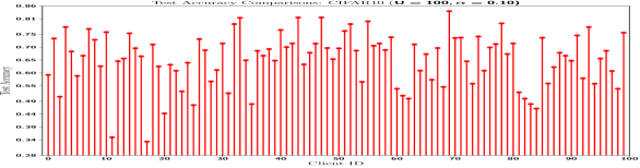
Figure 1: Globally trained model’s performance on CIFAR$10$: $65.36\%$, $83.93\%$ and $33.33\%$ mean, maximum and minimum test accuracy, respectively, across $100$ clients, when data samples are distributed following $\mathrm{Dir}(\boldsymbol{\alpha}=\mathbf{0.1})$ [4]

I-A State of the Art

Many recent works extended the idea of SL [7] into variants of FL [1] algorithms [11, 13, 12, 14, 15, 16, 17]. Xu et al. proposed a split federated learning (SFL) algorithm leveraging a single server with distributed clients [11]. In particular, the authors assumed that the client-side model is aggregated only after finishing the local rounds, while the server can aggregate the server-side models in each local training round. Liu et al. proposed hybrid SFL, where a part of the clients train their entire models locally, while others collaborate with their serving base station (BS) to train their respective model following SL [13]. Ao et al. proposed SFL assuming the BS selects a subset of the clients to participate in model training [16]. In particular, [16] jointly optimizes client scheduling, power allocation, and cut layer selection to minimize a weighted utility function that strikes a balance between the training time and energy overheads.

Khan et al. proposed an HSFL algorithm leveraging hierarchical federated learning (HFL) and SL [12]. In particular, the authors aimed at optimizing the latency and energy cost associated with HSFL. Liao et al. proposed a similar HSFL algorithm that partitioned clients into different clusters [14]. The authors leveraged grouping the clients into appropriate clusters to tame the system heterogeneity. However, statistical data heterogeneity is well known to cause client drifts [18]. Lin et al. proposed a parallel SL algorithm that jointly optimized the cut layer splitting strategy, radio allocation, and power control to minimize per-round training latency [17]. As opposed to SFL, parallel SL did not aggregate client-side models.

On the personalized SFL side, Han et al. proposed weighted aggregation of the local and global models during the local model synchronization phase [19]. Similar ideas were also explored in [20], where the authors mixed partial global model parameters with the local model parameters during the local model synchronization. However, [20] did not explore SL. Chen et al. proposed a 3-stage U-shape split learning algorithm [21]. More specifically, the authors divided the model into front, middle and back parts, where the clients retained the front and back parts, while the server had the bulky middle part. Such U-shape architecture incurs additional communication burden compared to [19].

I-B Research Gaps and Our Contributions

The existing studies [11, 13, 12, 14, 15, 16, 17] considered SFL, HSFL and parallel SL extensively without addressing the need for personalization. While [19, 21] addressed joint personalization and split FL, these works were based on a traditional single server with distributed clients case. Therefore, weighted aggregation in multi-tier/hierarchical networks may lose personalization ability if the learning rate is not significantly low. Moreover, training the entire model is proven to have poor personalization capability [22]: even though the model was split into client-side and server-side parts, all model blocks on both sides of the models were updated in [19, 21].

Motivated by the above facts, we propose a PHSFL algorithm that integrates HFL and SL. The designed algorithm lets distributed clients train only the body part of the ML model to learn feature representations while keeping the output layer (e.g., the classifier) frozen during the training process inspired by the fact that globally trained model works great for generalization, while performs poorly for personalization. Besides, we perform extensive theoretical analysis to find the theoretical bound of the average global gradient norm of the global loss function. Our simulation results suggest that while the global trained model performs similarly to HSFL in generalization, with the similarly fine-tuned models for both cases, our proposed solution achieves significantly better personalization performance.

II System Model and Preliminaries

II-A Network Model

We consider a hierarchical wireless network with $\mathcal{B}=\{b\}_{b=0}^{B-1}$ edge servers and a central server (CS). Each ES has $\mathcal{U}_{b}=\{u\}_{u=0}^{U_{b}-1}$ (wireless) clients. Besides, we have $\mathcal{U}_{b}\bigcap\mathcal{U}_{b^{\prime}\neq b}=\varnothing$ and $\mathcal{U}\coloneqq\bigcup_{b=0}^{B-1}\mathcal{U}_{b}$. Denote client $u$’s local dataset by $\mathcal{D}_{u,\mathrm{ft}}=\{\mathbf{x}_{n}\}_{n=0}^{\mathrm{D}_{u}-1}$ that only contains the feature set. Furthermore, let us denote the corresponding label set by $\mathcal{D}_{u,\mathrm{lb}}=\{\mathbf{y}_{n}\}_{n=0}^{\mathrm{D}_{u}-1}$, which belongs to the ES. Moreover, we assume that the clients are resource-constrained and do not own the entire dataset or ML model. We also assume that the clients have perfect communications with the ESs.

II-B Preliminaries: Hierarchical Federated Learning (HFL)

Similar to the typical single-server-based FL, we want to train a ML model $\mathbf{w}$ collaboratively using the clients $\mathcal{U}$ and ESs $\mathcal{B}$ in HFL. In particular, each global round has $\kappa_{1}$ edge rounds, and each of these edge rounds has $\kappa_{0}$ local training rounds, i.e., mini-batch stochastic gradient descent (SGD) steps. Let us denote the indices of the global, edge and local rounds by $t_{2}$, $t_{1}$ and $t_{0}$, respectively. We thus keep track of the SGD steps by

$$t\coloneqq t_{2}\kappa_{1}\kappa_{0}+t_{1}\kappa_{0}+t_{0}.$$ (1)

Denote the global ML model at the CS, the edge model at the $b^{\mathrm{th}}$ BS/ES and the local model of user $u\in\mathcal{U}_{b}$ by $\mathbf{w}^{t}$, $\mathbf{w}_{b}^{t}$, and $\mathbf{w}_{u}^{t}$ respectively. It is worth noting that the global and edge models are not updated in every SGD step in HFL, as described below.

At the start of each global round $t_{2}$, i.e., $(t\mod[t_{2}\kappa_{1}\kappa_{0}+t_{1}\kappa_{0}+t_{0}])=0$, the global model $\mathbf{w}^{t}$ is broadcasted to all ESs. These ESs then start their respective edge rounds $t_{1}\ni t=t_{2}\kappa_{1}\kappa_{0}+t_{1}\kappa_{0}$ by synchronizing their edge models $\mathbf{w}_{b}^{t}\leftarrow\mathbf{w}^{t}$, followed by broadcasting their edge models to their respective clients $\mathcal{U}_{b}$. Before the local training, the clients synchronize their local models at $\bar{t}_{0}\coloneqq t_{2}\kappa_{2}\kappa_{1}+t_{1}\kappa_{0}$, as $\mathbf{w}_{u}^{\bar{t}_{0}}\leftarrow\mathbf{w}_{b}^{\bar{t}_{0}}$. The clients want to minimize

$$f_{u}\big{(}\mathbf{w}_{u}^{\bar{t}_{0}}|\mathcal{D}_{u}\big{)}\coloneqq\frac{1}{|\mathcal{D}_{u,\mathrm{ft}}|}\sum\nolimits_{{\mathbf{x}_{a},y_{a}}\in\mathcal{D}_{u}}l(\mathbf{w}_{u}^{\bar{t}_{0}}|(\mathbf{x}_{a},y_{a})),$$ (2)

where $\mathcal{D}_{u}\coloneqq\{\mathcal{D}_{u,\mathrm{ft}},\mathcal{D}_{u,\mathrm{lb}}\}$ and $l(\mathbf{w}_{u}^{\bar{t}_{0}}|(\mathbf{x}_{a},y_{a})$ the loss function (e.g., cross entropy, mean square error, etc.) evaluated using ML model $\mathbf{w}_{u}^{\bar{t}_{0}}$ and training sample $(\mathbf{x}_{a},y_{a})$. Each user takes $\kappa_{0}$ SGD steps to minimize (2) as

$$\mathbf{w}_{u}^{\bar{t}_{0}+\kappa_{0}}=\mathbf{w}_{u}^{\bar{t}_{0}}-\eta\sum\nolimits_{t_{0}=0}^{\kappa_{0}-1}g_{u}(\mathbf{w}_{u}^{t_{0}}),$$ (3)

where $\eta$ is the step size and $g_{u}(\cdot)$ is the stochastic gradient Once $\kappa_{0}$ SGD steps get completed, each client offloads the trained model $\mathbf{w}_{u,b}^{\bar{t}_{0}+\kappa_{0}}$ to their respective associated ES, and the ES then aggregates the updated models as

$$\mathbf{w}_{b}^{\bar{t}_{0}+\kappa_{0}}=\sum\nolimits_{u\in\mathcal{U}_{b}}\alpha_{u}\cdot\mathbf{w}_{u}^{{\bar{t}_{0}}+\kappa_{0}},$$ (4)

where $0\leq\alpha_{u}\leq 1$ and $\sum_{u\in\mathcal{U}_{b}}\alpha_{u}=1$ for all $b\in\mathcal{B}$. This completes one edge round and hence, ES minimizes the following loss function

$$f_{b}(\mathbf{w})=\sum\nolimits_{u\in\mathcal{U}_{b}}\alpha_{u}f_{u}(\mathbf{w}).$$ (5)

Each ES repeats the above steps for $\kappa_{1}$ times and then sends the updated edge model to the CS at $t=t_{2}\kappa_{1}\kappa_{0}+\kappa_{1}\kappa_{0}$. The CS then updates the global model as

$$\mathbf{w}^{(t_{2}+1)\kappa_{1}\kappa_{0}}=\sum\nolimits_{b=0}^{B-1}\alpha_{b}\cdot\mathbf{w}_{b}^{t_{2}\kappa_{1}\kappa_{0}+\kappa_{1}\kappa_{0}},$$ (6)

where $0\leq\alpha_{b}\leq 1$ and $\sum_{b=0}^{B-1}\alpha_{b}=1$. This completes one global round, and hence, the CS minimizes the following global loss function

$$f(\mathbf{w})=\sum\nolimits_{b=0}^{B-1}\alpha_{b}f_{b}(\mathbf{w})=\sum\nolimits_{b=0}^{B-1}\alpha_{b}\sum\nolimits_{u\in\mathcal{U}_{b}}\alpha_{u}f_{u}(\mathbf{w}).$$ (7)

III Personalized Split Hierarchical FL

To mitigate the resource constraints and achieve good personalization ability, we propose a PHSFL algorithm that first trains a global model with SL and a frozen output/classifier layer and then lets the clients fine-tune only the classifier on their local training dataset.

III-A Proposed Personalized Split HFL: Global Model Training

First, we describe the global model training process with the following key steps.

III-A1 Step 1 - Global Round Initialization

At each global round $t_{2}$, the global model $\mathbf{w}^{t_{2}\kappa_{1}\kappa_{0}}$ is broadcasted to all ESs.

III-A2 Step 2 - Edge Round Initialization

At the start of the first edge round, i.e., $t_{1}=0$, each ES synchronizes its edge model as

$$\mathbf{w}_{b}^{t_{2}\kappa_{1}\kappa_{0}+t_{1}\kappa_{0}}\leftarrow\mathbf{w}^{t_{2}\kappa_{1}\kappa_{0}}.$$ (8)

Step 2.1 - Edge Model Splitting: Each ES then splits the model at the cut layer as $\mathbf{w}_{b}^{\bar{t}_{0}}\coloneqq[\mathbf{w}_{b,0}^{\bar{t}_{0}};\mathbf{w}_{b,1}^{\bar{t}_{0}}]$ [7], where recall that $\bar{t}_{0}\coloneqq t_{2}\kappa_{1}\kappa_{0}+t_{1}\kappa_{0}$. While SL helps us to tackle the resource constraints, it does not ensure model personalization. As such, we first split the server-side model into two parts as $\mathbf{w}_{b,1}^{\bar{t}_{0}}=[\mathbf{w}_{b,1,\mathrm{bd}}^{\bar{t}_{0}};\mathbf{w}_{b,1,\mathrm{hd}}^{\bar{t}_{0}}]$, where $\mathbf{w}_{b,1,\mathrm{bd}}^{\bar{t}_{0}}$ is the body part that works as the feature extractor, $\mathbf{w}_{b,1,\mathrm{hd}}^{\bar{t}_{0}}$ is the head part, i.e., the output layer/classifier that generates the final output.

Step 2.2 - Freeze Server-Side Classifier: Following [22], we randomly initiate $\mathbf{w}_{b,1,\mathrm{hd}}^{\bar{t}_{0}}$ and freeze it during the training phase, i.e., $\mathbf{w}_{b,1,\mathrm{hd}}^{\bar{t}_{0}}$ is never updated during the model training phase.

Step 2.3 - Edge Model Broadcasting: Each ES then only broadcasts the client-side model parts $\mathbf{w}_{b,0}^{\bar{t_{0}}}$ to its associated users $\mathcal{U}_{b}$.

III-A3 Step 3 - Local Model Training

Since clients can only train the client-side model, local training requires information exchange between the client-side and server-side models. This is achieved through the following key steps.

Step 3.1 - Local Model Synchronization: Each clients in $\mathcal{U}_{b}$ synchronizes their respective local model, i.e., the client-side model part, using the received broadcasted model as $\mathbf{w}_{u,0}^{\bar{t}_{0}}\leftarrow\mathbf{w}_{b,0}^{\bar{t}_{0}}$. The ES initializes the server-side model parts for each $u\in\mathcal{U}_{b}$ as $\mathbf{w}_{u,1}^{\bar{t}_{0}}\leftarrow\mathbf{w}_{b,1}^{\bar{t}_{0}}$ simultaneously.

Step 3.2 - Forward Propagation of Client-Side Model: Given input data $\mathbf{x}_{n}$, the output of the activation function is a mapping of the input data and corresponding weight matrices of the layers in the client-side model. More specifically, we consider mini-batch SGD, where each client randomly selects $N$, i.e., mini-batch size, samples, and feeds that as the input to the model. Denote the indices of the randomly selected training features by $\mathcal{N}$. As such, denote the output at the cut-layer during the $t_{0}^{\mathrm{th}}$ local round for a mini-batch of $N$ training samples as $\mathbf{o}_{u,\mathrm{fp}}^{t_{0}}\coloneqq\tilde{f}\big{(}\mathbf{w}_{u,0}^{t_{0}}|\{\mathbf{x}_{n}\}_{n=0}^{N}\big{)}$, where $\mathbf{x}_{n}\sim\mathcal{D}_{u,\mathrm{ft}}$ and $\tilde{f}(\mathbf{w}_{u,0}^{\bar{t}_{0}}|\{\mathbf{x}_{n}\}_{n=0}^{N})$ represents the forward propagation with respect to model $\mathbf{w}_{u,0}^{\bar{t}_{0}}$ conditioned on the data samples $\{\mathbf{x}_{n}\}_{n=0}^{N}$.

Step 3.4 - Transmission of Cut-Layer’s Output: Each client offloads $\mathbf{o}_{u,\mathrm{fp}}^{\bar{t}_{0}}$ and the set of (randomly sampled) indices $\mathcal{N}$ to its associated ES. It is worth noting that existing HSFL algorithms usually require offloading the corresponding labels to the associated server(s), which may reveal private information.

Step 3.5 - Forward Propagation of Server-Side Model: Each ES takes $\mathbf{o}_{u,\mathrm{fp}}^{\bar{t}_{0}}$ as input and computes the forward propagation of the server-side model part that gives the predicted label $\hat{\mathbf{Y}}\coloneqq\tilde{f}\big{(}\mathbf{w}_{u,1}^{\bar{t}_{0}}|\mathbf{o}_{u,\mathrm{fp}}^{\bar{t}_{0}},\mathcal{N}\big{)}$. The ES extracts the original labels using the received indices $\mathcal{N}$. Given the original label for the sample $\mathbf{x}_{n}$ is $\mathbf{y}_{n}$, the loss associated to this particular sample is denoted by $l\big{(}\mathbf{y}_{n},\hat{\mathbf{Y}}[n]\big{)}=l\big{(}\mathbf{y}_{n},\tilde{f}\big{(}\mathbf{w}_{u,1}^{\bar{t}_{0}}|\mathbf{o}_{u,\mathrm{fp}}^{\bar{t}_{0}},\mathcal{N}\big{)}[n]\big{)}$. As such, we write the loss function associated with a mini-batch as

$$f_{u}\big{(}\mathbf{w}_{u,1}^{\bar{t}_{0}}|\mathbf{o}_{u,\mathrm{fp}}^{\bar{t}_{0}}\big{)}\coloneqq[1/N]\sum\nolimits_{n\in\mathcal{N}}l(\mathbf{y}_{n},\hat{\mathbf{Y}}[n])$$

$$\qquad\qquad=[1/N]l\sum\nolimits_{n\in\mathcal{N}}\big{(}\mathbf{y}_{n},\tilde{f}\big{(}\mathbf{w}_{u,1}^{\bar{t}_{0}}|\mathbf{o}_{u,\mathrm{fp}}^{\bar{t}_{0}},\mathcal{N}\big{)}[n]\big{)}.$$ (9)

Step 3.6 - Back Propagation of Server-Side Model: In order to minimize (III-A3), the server first performs backpropagation using the server-side model part as

$$\mathbf{w}_{u,1}^{\bar{t}_{0}+1}=\mathbf{w}_{u,1}^{\bar{t}_{0}}-\eta\big{[}g_{u}\big{(}\mathbf{w}_{u,1}^{\bar{t}_{0}}|\mathbf{o}_{u,\mathrm{fp}}^{\bar{t}_{0}}\big{)}\big{]}_{\mathbf{w}_{u,1}^{\bar{t}_{0}}},$$ (10)

where $\eta$ is the learning rate and $\big{[}g_{u}\big{(}\mathbf{w}_{u,1}^{\bar{t}_{0}}|\mathbf{o}_{u,\mathrm{fp}}^{\bar{t}_{0}}\big{)}\big{]}_{\mathbf{w}_{u,1}^{\bar{t}_{0}}}$, represents the stochastic gradient with respect to the server-side model parameters $\mathbf{w}_{u,1}^{\bar{t}_{0}}$. Since $\mathbf{w}_{u,1,\mathrm{hd}}^{\bar{t}_{0}}$ is frozen and $\mathbf{w}_{u,1}^{\bar{t}_{0}}=[\mathbf{w}_{u,1,\mathrm{bd}}^{\bar{t}_{0}};\mathbf{w}_{u,1,\mathrm{hd}}^{\bar{t}_{0}}]$, (10) implies the following

$$\mathbf{w}_{u,1,\mathrm{bd}}^{\bar{t}_{0}+1}=\mathbf{w}_{u,1,\mathrm{bd}}^{\bar{t}_{0}}-\eta\big{[}g_{u}\big{(}\mathbf{w}_{u,1,\mathrm{bd}}^{\bar{t}_{0}}|\mathbf{o}_{u,\mathrm{fp}}^{\bar{t}_{0}}\big{)}\big{]}_{\mathbf{w}_{u,1,\mathrm{bd}}^{\bar{t}_{0}}}.$$ (11)

$$\mathbf{w}_{u,1,\mathrm{hd}}^{\bar{t}_{0}+1}=\mathbf{w}_{u,1,\mathrm{hd}}^{\bar{t}_{0}}-0\times\big{[}g_{u}\big{(}\mathbf{w}_{u,1,\mathrm{hd}}^{\bar{t}_{0}}|\mathbf{o}_{u,\mathrm{fp}}^{\bar{t}_{0}}\big{)}\big{]}_{\mathbf{w}_{u,1,\mathrm{hd}}^{\bar{t}_{0}}},$$ (12)

where a learning rate of $0$ means the $\mathbf{w}_{u,1\mathrm{hd}}^{\bar{t}_{0}}$ is not getting updated. Besides, we do not need to set $\eta=0$ explicitly for the classifier during the model training phase since we can disable the gradient computation for the classifier in almost all popular ML libraries like PyTorch and TensorFlow. Furthermore, the gradients are calculated using the chain rule. Denote the gradient of the server-side input layer, i.e., the layer that receives the cut-layer output $\mathbf{o}_{u,\mathrm{fp}}^{\bar{t}_{0}}$ as client-side model’s input by $\mathbf{o}_{u,\mathrm{bp}}^{\bar{t}_{0}}$.

Step 3.7 - Transmission of Server-Side Cut-Layer’s Gradient: The ES then transmits the gradient $\mathbf{o}_{u,\mathrm{bp}}^{\bar{t}_{0}}$ to the client to compute the gradients of the client-side model $\mathbf{w}_{u,0}^{\bar{t}_{0}}$ using the chain rule.

Step 3.8 - Back Propagation of Client-Side Model: Each client then performs backpropagation to compute the gradients that minimizes the loss function as

$$\mathbf{w}_{u,0}^{\bar{t}_{0}+1}=\mathbf{w}_{u,0}^{\bar{t}_{0}}-\eta\big{[}g_{u}\big{(}\mathbf{w}_{u,1}^{\bar{t}_{0}}|\mathbf{o}_{u,\mathrm{fp}}^{\bar{t}_{0}}\big{)}\big{]}_{\mathbf{w}_{u,0}^{\bar{t}_{0}}|\mathbf{o}_{u,\mathrm{bp}}^{\bar{t}_{0}}},$$ (13)

where the notation $\big{[}g_{u}\big{(}\mathbf{w}_{u,1}^{\bar{t}_{0}}|\mathbf{o}_{u,\mathrm{fp}}^{\bar{t}_{0}}\big{)}\big{]}_{\mathbf{w}_{u,0}^{\bar{t}_{0}}|\mathbf{o}_{u,\mathrm{bp}}^{\bar{t}_{0}}}$ represents the stochastic gradient of the loss function with respect to $\mathbf{w}_{u,0}^{\bar{t}_{0}}$ that depends on the gradient at cut-layer $\mathbf{o}_{u,\mathrm{bp}}^{\bar{t}_{0}}$, which is available to the client. Therefore, the client can complete the gradient with respect to its client-side model parameters using chain rule.

Steps 3.2 - 3.8 are repeated for $\mathrm{N}$ mini-batches, which completes one local training epoch. Each client performs $\kappa_{0}$ local epochs, which complete the local training.

III-A4 Step 4 - Trained Client-Side Model Offloading

All clients offload their respective trained client-side model $\mathbf{w}_{u,0}^{\bar{t}_{0}+\kappa_{0}}$ to their associated ES.

III-A5 Step 5 - Edge Aggregation

Each ES then aggregates the client-side and server-side models as

$$\mathbf{w}_{b,0}^{\bar{t}_{0}+\kappa_{0}}=\mathbf{w}_{b,0}^{t_{2}\kappa_{1}\kappa_{0}+(t_{1}+1)\kappa_{0}}=\sum\nolimits_{u=0}^{U_{b}-1}\alpha_{u}\mathbf{w}_{u,0}^{\bar{t}_{0}+\kappa_{0}}.$$ (14)

$$\mathbf{w}_{b,1}^{\bar{t}_{0}+\kappa_{0}}=\mathbf{w}_{b,1}^{t_{2}\kappa_{1}\kappa_{0}+(t_{1}+1)\kappa_{0}}=\sum\nolimits_{u=0}^{U_{b}-1}\alpha_{u}\mathbf{w}_{u,1}^{\bar{t}_{0}+\kappa_{0}}.$$ (15)

Each ES repeats Step 2.2 to Step 5 $\kappa_{1}$ times and then sends the updated edge model $\mathbf{w}_{b}^{t_{2}\kappa_{1}\kappa_{2}+\kappa_{1}\kappa_{2}}=[\mathbf{w}_{b,0}^{t_{2}\kappa_{1}\kappa_{2}+\kappa_{1}\kappa_{2}};\mathbf{w}_{b,1}^{t_{2}\kappa_{1}\kappa_{2}+\kappa_{1}\kappa_{2}}]$ to the CS.

III-A6 Step 6 - Global Aggregation

Upon receiving the updated edge models, the CS aggregates these updated models and updates the global model as

$$\mathbf{w}^{(t_{2}+1)\kappa_{1}\kappa_{0}}=\sum\nolimits_{b=0}^{B-1}\alpha_{b}\mathbf{w}_{b}^{t_{2}\kappa_{1}\kappa_{0}+\kappa_{1}\kappa_{0}}.$$ (16)

This concludes one global round. The above steps are repeated for $t_{2}=0,1,\dots,R-1$ rounds.

III-B Personalized Split HFL: Fine-Tuning of Global Trained Model

Once the globally trained model $\mathbf{w}^{*}$ is obtained, the CS broadcasts it to all ESs. We assume the clients will fine-tune the trained model for $\{k\}_{k=0}^{K-1}$ SGD steps. The ES then splits the model as $\mathbf{w}_{b}^{k}\coloneqq[\mathbf{w}_{b,0}^{k};\mathbf{w}_{b,1}^{k}]$. It then broadcasts the trained client-side model to all clients and initialize the server-side model as $\mathbf{w}_{u,1}^{k}=[\mathbf{w}_{u,1,\mathrm{bd}}^{k};\mathbf{w}_{u,1,\mathrm{hd}}^{k}]$. The client computes its forward propagation output $\mathbf{o}_{u,\mathrm{fp}}^{k}$ and shares that with the ES. The ES then takes a SGD step to fine-tune the head/classifier as

$$\mathbf{w}_{u,1,\mathrm{hd}}^{k+1}=\mathbf{w}_{u,1,\mathrm{hd}}^{k}-\tilde{\eta}\big{[}g_{u}\big{(}\mathbf{w}_{u,1,\mathrm{hd}}^{k}|\mathbf{o}_{u,\mathrm{fp}}^{k}\big{)}\big{]}_{\mathbf{w}_{u,1,\mathrm{hd}}^{k}},$$ (17)

where $\tilde{\eta}$ is the learning rate that can differ from $\eta$. The body part and the client-side model weights remain as-it-is in $\mathbf{w}^{*}$. The above steps are repeated for $K$ times, which gives the personalized classifier as $\mathbf{w}_{u,1,\mathrm{hd}}^{K}$. Hence, the entire personalized model of the $u^{\mathrm{th}}$ user can be expressed as $\mathbf{w}_{u}^{K}=[\mathbf{w}_{b,0}^{*};[\mathbf{w}_{b,1,\mathrm{bd}}^{*};\mathbf{w}_{b,1,\mathrm{hd}}^{K}]]$.

IV Theoretical Analysis

For notational simplicity, we use the notation $f_{u}(\mathbf{w}_{u}^{t})$ to represent client’s loss function $f_{u}\big{(}\mathbf{w}_{u,1}^{t}|\mathbf{o}_{u,\mathrm{fp}}^{t}\big{)}$ and $g_{u}(\mathbf{w}_{u}^{t})$ to represent $\left[\big{[}g_{u}\big{(}\mathbf{w}_{u,1}^{t}|\mathbf{o}_{u,\mathrm{fp}}^{t}\big{)}\big{]}_{\mathbf{w}_{u,0}^{t}|\mathbf{o}_{u,\mathrm{bp}}^{t}};\big{[}g_{u}\big{(}\mathbf{w}_{u,1}^{t}|\mathbf{o}_{u,\mathrm{fp}}^{t}\big{)}\big{]}_{\mathbf{w}_{u,1}^{t}}\right]$ throughout the rest of the paper.

IV-A Assumptions

We make the following standard assumptions [23, 8, 24, 25, 26]

Assumption 1 (Smoothness).

The loss functions are $\beta$-Lipschitz smooth, i.e., for some $\beta>0$, $\|\nabla f(\mathbf{w})-\nabla f(\mathbf{w}^{\prime})\|\leq\beta\|\mathbf{w}-\mathbf{w}^{\prime}\|$, where $\|\cdot\|$ is the $L_{2}$ norm, for all loss functions.

Assumption 2 (Unbiased gradient with bounded variance).

The mini-batch stochastic gradient calculated using client’s randomly sampled mini-batch $\zeta$ is unbiased, i.e., $\mathbb{E}_{\zeta\sim\mathcal{D}_{u}}\left[g_{u}(\mathbf{w})\right]=\nabla f_{u}(\mathbf{w})$, where $\mathbb{E}[\cdot]$ is the expectation operator. Besides, the variance of the gradients is bounded, i.e., $\mathbb{E}_{\zeta\sim\mathcal{D}_{u}}\left[\|\nabla f_{u}(\mathbf{w})-g_{u}(\mathbf{w})\|^{2}\right]\leq\sigma^{2}$, for some $\sigma\geq 0$ and all $u\in\mathcal{U}$.

Assumption 3 (Bounded gradient divergence).

The divergence between (a) local and ES loss functions and (b) ES and global loss functions are bounded as

$$\sum\nolimits_{u\in\mathcal{U}_{b}}\alpha_{u}\|\nabla f_{u}(\mathbf{w})-\nabla f_{b}(\mathbf{w})\|^{2}\leq\epsilon_{0}^{2},$$ (18)

$$\sum\nolimits_{b=1}^{B}\alpha_{b}\|\nabla f_{b}(\mathbf{w})-\nabla f(\mathbf{w})\|^{2}\leq\epsilon_{1}^{2},$$ (19)

for some $\epsilon_{0}\leq 0$, $\epsilon_{1}\leq 0$ and all $u$ and $b$.

Additionally, since the global and edge models do not exist in every SGD step $t$, following standard practice [8, 24], we assume that virtual copies of these models exist, denoted by $\bar{\mathbf{w}}^{t}$ and $\bar{\mathbf{w}}_{b}^{t}$, respectively. Moreover, the above assumptions also apply to these virtual models.

IV-B Convergence Analysis

Theorem 1.

Suppose the above assumptions hold. Then, if the learning rate satisfies $\eta<\frac{1}{2\sqrt{5}\beta\kappa_{1}\kappa_{0}}$, the average global gradient norm is upper bounded by

$$\!\!\!\!\frac{1}{T}\sum_{t=0}^{T-1}\mathbb{E}\left[\left\|\nabla f(\bar{\mathbf{w}}^{t})\right\|^{2}\right]\leq\frac{2\left(\mathbb{E}\left[f\left(\bar{\mathbf{w}}^{0}\right)\right]-\mathbb{E}\left[f\left(\bar{\mathbf{w}}^{T}\right)\right]\right)}{\eta T}+$$

$$\!\!\!\!\beta\eta\sigma^{2}\sum\nolimits_{b=0}^{B-1}\alpha_{b}^{2}\sum\nolimits_{u\in\mathcal{U}_{b}}\alpha_{u}^{2}+\left(\Gamma_{0}+\Gamma_{1}\right)\sigma^{2}+\tilde{\Gamma}_{0}\epsilon_{0}^{2}+\tilde{\Gamma_{1}}\epsilon_{1}^{2},\!\!$$ (20)

where $\Gamma_{0}\coloneqq 4\beta^{2}\eta^{2}\kappa_{0}^{2}-4\beta^{2}\eta^{2}\kappa_{0}^{2}\sum_{b=0}^{B-1}\alpha_{b}\sum_{u\in\mathcal{U}_{b}}\alpha_{u}^{2}$, $\Gamma_{1}\coloneqq 80\kappa_{1}^{2}\beta^{4}\eta^{4}\kappa_{0}^{4}+4\kappa_{1}\kappa_{0}\beta^{2}\eta^{2}\sum_{b=0}^{B-1}\alpha_{b}\sum_{u\in\mathcal{U}_{b}}\alpha_{u}^{2}-4\kappa_{1}\kappa_{0}\beta^{2}\eta^{2}\sum_{b=0}^{B-1}\alpha_{b}^{2}\sum_{u\in\mathcal{U}_{b}}\alpha_{u}^{2}-80\kappa_{1}^{2}\beta^{4}\eta^{4}\kappa_{0}^{4}\sum_{b=0}^{B-1}\alpha_{b}\sum_{u\in\mathcal{U}_{b}}\alpha_{u}^{2}$, $\tilde{\Gamma}_{0}\coloneqq 12\beta^{2}\eta^{2}\kappa_{0}^{2}\big{(}1+20\kappa_{0}^{2}\kappa_{1}^{2}\beta^{2}\eta^{2}\big{)}$ and $\tilde{\Gamma}_{1}\coloneqq 20\beta^{2}\eta^{2}\kappa_{1}^{2}\kappa_{0}^{2}$.

Proof.

The proof is left in our online supplementary materials [27]. ∎

Remark 1.

The first two terms in (1) are analogous to standard SGD: the first term captures the diminishing loss, while the second term appears from the bounded variance assumption of the stochastic gradients. The third term also appears due to the bounded variance assumption of the stochastic gradients: $\Gamma_{0}$ and $\Gamma_{1}$ are the contribution from user-ES and ES-CS hierarchy levels, respectively. The fourth and fifth terms capture the divergence between the user-ES and ES-CS loss functions, respectively, and arise from the statistical data heterogeneity.

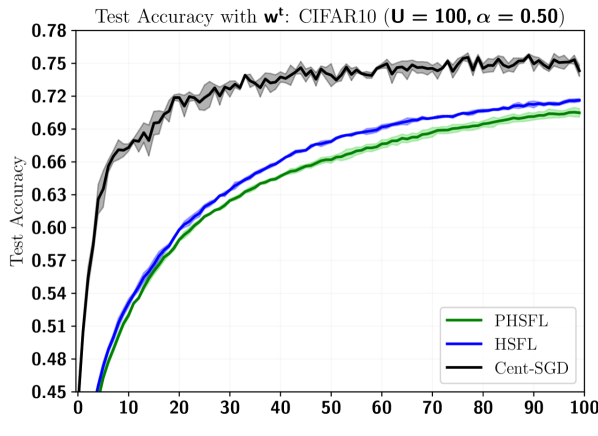
(a) Test accuracy with $\mathbf{w}^{t}$

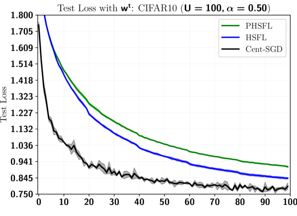
(b) Test loss with $\mathbf{w}^{t}$

Figure 2: Test performance comparisons on CIFAR$10$ across $U=100$ users, when $\mathrm{Dir}(\boldsymbol{\alpha}=\mathbf{0.5)}$

V Simulation Results and Discussions

V-A Simulation Setting

We consider $4$ BSs/ESs, each serving $25$ users. For simplicity, we assume perfect communication between the users and the BSs for information exchange. Besides, we use a symmetric Dirichlet distribution ${\tt Dir(\boldsymbol{\alpha})}$, where $\boldsymbol{\alpha}$ is the concentration parameter and determines the skewness, to distribute the training and test samples across these $U=100$ users following a similar strategy as in [4]. We use the image classification task with the widely popular CIFAR$10$ dataset to evaluate the performance of our proposed PHSFL algorithm. However, this can be easily extended to other applications and/or datasets.

We use a simple convolutional neural network (CNN) model as our ML model $\mathbf{w}$ that has the following architecture: Conv2d (#Channels, $64$) $\rightarrow$ ReLU() $\rightarrow$ MaxPool2d $\rightarrow$ Conv2d($64$,$128$) $\rightarrow$ ReLU() $\rightarrow$ MaxPool2d $\rightarrow$ FC($512$, $256$), $\rightarrow$ ReLU() $\rightarrow$ FC($256$, #Labels). The model is split after the first MaxPool2d layer. As such, the client-side model part is Conv2d (#Channels, $64$) $\rightarrow$ ReLU() $\rightarrow$ MaxPool2d. The rest of the model blocks belong to the server-side model parts, where the classifier/head is the output layer, i.e., FC($256$, #Labels). Finally, for the model training, we use SGD optimizer with $\eta=0.01$, $\mathrm{N}=32$, $N=5$, $\kappa_{0}=5$, $\kappa_{1}=3$ and $R=100$.

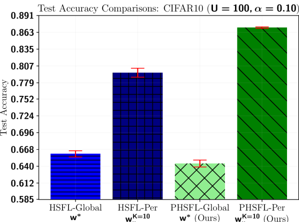
(a) Test Accuracy Comparisons

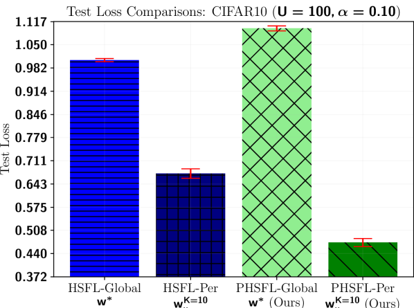
(b) Test Loss Comparisons

Figure 3: Test performance comparisons on CIFAR$10$ across $U=100$ users, when $\mathrm{Dir}(\boldsymbol{\alpha}=\mathbf{0.1)}$

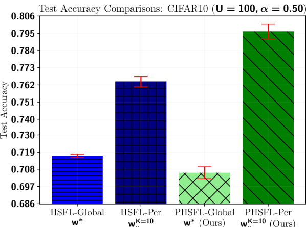
(a) Test Accuracy Comparisons

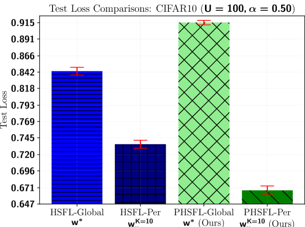
(b) Test Loss Comparisons

Figure 4: Test performance comparisons on CIFAR$10$ across $U=100$ users, when $\mathrm{Dir}(\boldsymbol{\alpha}=\mathbf{0.5)}$

V-B Performance Comparisons

In order to evaluate the performance, we adopt a HSFL learning baseline based on [12, 14]. More specifically, we assume the same system configurations, data distributions, and perfect communication between the clients and ESs as in our proposed PHSFL algorithm. Moreover, we also use a centralized SGD baseline to get the performance upper bound, assuming a Genie has access to all data samples. The SGD algorithm iterates over the entire dataset (using $[\bigcup_{u\in\mathcal{U}}|\mathcal{D}_{u}|]/N$ mini-batches) for $R=100$ epochs.

First, we investigate the generalization performance with the globally trained model $\mathbf{w}^{t}$. Intuitively, as only the body parts of the model get trained with respect to a randomly initialized classifier, the classification results may not be as accurate as when the entire model gets trained. This is due to the fact that the head/classifier does not update the initial weights as training progresses, as shown in (12). However, recall that our sole interest lies in having personalized models for the clients. Our simulation results in Fig. 2 also validate this intuition. We observe a small gap between the generalized model performances from these two algorithms. For example, upon finishing $R=100$ global rounds, PHSFL and HSFL have $0.7049\pm 0.0039$ and $0.7163\pm 0.0015$ test accuracies, respectively. Besides, the test losses are $0.9104\pm 0.0053$ and $0.8432\pm 0.0053$, respectively, for PHSFL and HSFL. Moreover, both of these two algorithms have some clear performance deviations from the centralized SGD baseline, which is expected since they do not have access to the entire training dataset.

We now investigate the personalized models that are fine-tuned from the globally trained models with PHSFL and HSFL algorithms. In particular, we fine-tune the classifier/head of the model using $K=10$ SGD steps following the steps described in Section III-B. Note that since a higher skewness in the data distribution yields degraded generalized performance, model personalization shall benefit the most in such cases. Regardless of the data skewness, we expect PHSFL to perform better since it only learns the feature representations using the same classifier: since the features have similarities, severe data heterogeneity may not influence the lower model blocks. However, since HSFL updates all model blocks, data heterogeneity may affect the weights of the classifier/head, which may complicate fine-tuning the global model with a small $K$.

To understand the impact of non-IID data distributions, we consider two cases: $\mathrm{Dir}(\boldsymbol{\alpha}=\mathbf{0.1})$ and $\mathrm{Dir}(\boldsymbol{\alpha}=\mathbf{0.5})$. Note that smaller $\boldsymbol{\alpha}$ means more skewed data distribution. Our simulation results show the above trends in Figs. 3 and 4. When $\boldsymbol{\alpha}=\mathbf{0.1}$, we observe that the mean test accuracies from the global models are $0.6606\pm 0.0052$ and $0.64458\pm 0.0058$, respectively, for HSFL and PHSFL, while the corresponding test losses are $1.0049\pm 0.0046$ and $1.0975\pm 0.0073$. However, the personalized mean test accuracies are $0.7958\pm 0.0075$ and $0.8708\pm 0.0012$, while the test losses are $0.6735\pm 0.0138$ and $0.4721\pm 0.0118$, respectively, for HSFL and PHSFL. Therefore, our proposed PHSFL solution has $9.43\%$ and $42.68\%$ improvement in test accuracy and test loss over HSFL. Besides, when $\boldsymbol{\alpha}=\mathbf{0.5}$, the personalized models have $4.75\%$ and $9.03\%$ mean test accuracy improvement over the generalized global trained models, respectively, for HSFL and PHSFL.

VI Conclusion

We proposed a PHSFL algorithm that leverages SL and HFL and enables training an ML model with resource-constrained distributed clients in heterogeneous wireless networks. Our proposed algorithm trains the model to learn feature representations with a fixed classifier that never gets trained during the training phase. The fine-tuned classifier with the remaining trained global model blocks shows significant personalization performance improvement over other existing algorithms.

References

- [1] B. McMahan, E. Moore, D. Ramage, S. Hampson, and B. A. y. Arcas, ‘‘Communication-Efficient Learning of Deep Networks from Decentralized Data,’’ in Proc. AIStats. PMLR, 2017.
- [2] A. Hard, K. Rao, R. Mathews, S. Ramaswamy, F. Beaufays, S. Augenstein, H. Eichner, C. Kiddon, and D. Ramage, ‘‘Federated learning for mobile keyboard prediction,’’ arXiv preprint arXiv:1811.03604, 2018.
- [3] P. Kairouz et al., ‘‘Advances and open problems in federated learning,’’ Foundations and trends® in machine learning, vol. 14, no. 1--2, pp. 1--210, 2021.
- [4] M. F. Pervej, R. Jin, and H. Dai, ‘‘Resource constrained vehicular edge federated learning with highly mobile connected vehicles,’’ IEEE J. Sel. Areas Commun., vol. 41, no. 6, pp. 1825--1844, 2023.
- [5] M. Chen, Z. Yang, W. Saad, C. Yin, H. V. Poor, and S. Cui, ‘‘A joint learning and communications framework for federated learning over wireless networks,’’ IEEE Trans. Wireless Commun., vol. 20, no. 1, pp. 269--283, 2020.
- [6] Z. Lin, G. Qu, X. Chen, and K. Huang, ‘‘Split learning in 6g edge networks,’’ IEEE Wireless Commun., vol. 31, no. 4, pp. 170--176, 2024.
- [7] P. Vepakomma, O. Gupta, T. Swedish, and R. Raskar, ‘‘Split learning for health: Distributed deep learning without sharing raw patient data,’’ arXiv preprint arXiv:1812.00564, 2018.
- [8] M. F. Pervej, R. Jin, and H. Dai, ‘‘Hierarchical federated learning in wireless networks: Pruning tackles bandwidth scarcity and system heterogeneity,’’ IEEE Trans. Wireless Commun., vol. 23, no. 9, pp. 11 417--11 432, 2024.
- [9] A. Vaswani et al., ‘‘Attention is all you need,’’ Advances in NeurIPS, 2017.
- [10] Z. Chen, Z. Zhang, and Z. Yang, ‘‘Big AI models for 6G wireless networks: Opportunities, challenges, and research directions,’’ IEEE Wireless Commun., vol. 31, no. 5, pp. 164--172, 2024.
- [11] C. Xu, J. Li, Y. Liu, Y. Ling, and M. Wen, ‘‘Accelerating split federated learning over wireless communication networks,’’ IEEE Trans. Wireless Commun., vol. 23, no. 6, pp. 5587--5599, 2024.
- [12] L. U. Khan, M. Guizani, A. Al-Fuqaha, C. S. Hong, D. Niyato, and Z. Han, ‘‘A joint communication and learning framework for hierarchical split federated learning,’’ IEEE Internet Things J., vol. 11, no. 1, pp. 268--282, 2024.
- [13] X. Liu, Y. Deng, and T. Mahmoodi, ‘‘Wireless distributed learning: A new hybrid split and federated learning approach,’’ IEEE Trans. Wireless Commun., vol. 22, no. 4, pp. 2650--2665, 2022.
- [14] Y. Liao, Y. Xu, H. Xu, Z. Yao, L. Huang, and C. Qiao, ‘‘Parallelsfl: A novel split federated learning framework tackling heterogeneity issues,’’ arXiv preprint arXiv:2410.01256, 2024.
- [15] T. Xia, Y. Deng, S. Yue, J. He, J. Ren, and Y. Zhang, ‘‘Hsfl: an efficient split federated learning framework via hierarchical organization,’’ in Proc. IEEE CNSM, 2022.
- [16] H. Ao, H. Tian, and W. Ni, ‘‘Federated split learning for edge intelligence in resource-constrained wireless networks,’’ IEEE Trans. Consumer Electronics, 2024.
- [17] Z. Lin, G. Zhu, Y. Deng, X. Chen, Y. Gao, K. Huang, and Y. Fang, ‘‘Efficient parallel split learning over resource-constrained wireless edge networks,’’ IEEE Trans. Mobile Comput., vol. 23, no. 10, pp. 9224--9239, 2024.
- [18] S. P. Karimireddy, S. Kale, M. Mohri, S. Reddi, S. Stich, and A. T. Suresh, ‘‘Scaffold: Stochastic controlled averaging for federated learning,’’ in Proc. ICML. PMLR, 2020.
- [19] D.-J. Han, D.-Y. Kim, M. Choi, C. G. Brinton, and J. Moon, ‘‘Splitgp: Achieving both generalization and personalization in federated learning,’’ in Proc. IEEE INFOCOM. IEEE, 2023.
- [20] B. Sun, H. Huo, Y. Yang, and B. Bai, ‘‘Partialfed: Cross-domain personalized federated learning via partial initialization,’’ Advances in NeurIPS, vol. 34, pp. 23 309--23 320, 2021.
- [21] H. Chen, X. Chen, L. Peng, and Y. Bai, ‘‘Personalized fair split learning for resource-constrained internet of things,’’ Sensors, vol. 24, no. 1, p. 88, 2023.
- [22] J. Oh, S. Kim, and S.-Y. Yun, ‘‘FedBABU: Toward enhanced representation for federated image classification,’’ in Proc. ICLR, 2022.
- [23] J. Wang, Q. Liu, H. Liang, G. Joshi, and H. V. Poor, ‘‘Tackling the objective inconsistency problem in heterogeneous federated optimization,’’ Advances in NeurIPS, vol. 33, pp. 7611--7623, 2020.
- [24] J. Wang, S. Wang, R.-R. Chen, and M. Ji, ‘‘Demystifying why local aggregation helps: Convergence analysis of hierarchical sgd,’’ in Proc. AAAI, vol. 36, no. 8, 2022, pp. 8548--8556.
- [25] M. F. Pervej and A. F. Molisch, ‘‘Resource-aware hierarchical federated learning in wireless video caching networks,’’ IEEE Trans. Wireless Commun., 2024.
- [26] R. Ye, M. Xu, J. Wang, C. Xu, S. Chen, and Y. Wang, ‘‘Feddisco: Federated learning with discrepancy-aware collaboration,’’ in Proc. ICML. PMLR, 2023.
- [27] M. F. Pervej, , and A. F. Molisch. (2024, Nov.) Personalized hierarchical split federated learning in wireless networks (supplementary materials). [Online]. Available: https://drive.google.com/file/d/1Wgbp1AeLc35vVFjzEH8108hqOVveyU99/view?usp=sharing