A novel study on the MUSIC-type imaging of small electromagnetic inhomogeneities in the limited-aperture inverse scattering problem

Won-Kwang Park parkwk@kookmin.ac.kr Department of Information Security, Cryptography, and Mathematics, Kookmin University, Seoul, 02707, Republic of Korea.
Abstract

We apply MUltiple SIgnal Classification (MUSIC) algorithm for the location reconstruction of a set of two-dimensional circle-like small inhomogeneities in the limited-aperture inverse scattering problem. Compared with the full- or limited-view inverse scattering problem, the collected multi-static response (MSR) matrix is no more symmetric (thus not Hermitian), and therefore, it is difficult to define the projection operator onto the noise subspace through the traditional approach. With the help of an asymptotic expansion formula in the presence of small inhomogeneities and the structure of the MSR-matrix singular vector associated with nonzero singular values, we define an alternative projection operator onto the noise subspace and the corresponding MUSIC imaging function. To demonstrate the feasibility of the designed MUSIC, we show that the imaging function can be expressed by an infinite series of integer-order Bessel functions of the first kind and the range of incident and observation directions. Furthermore, we identify that the main factors of the imaging function for the permittivity and permeability contrast cases are the Bessel function of order zero and one, respectively. This further implies that the imaging performance significantly depends on the range of incident and observation directions; peaks of large magnitudes appear at the location of inhomogeneities for permittivity contrast case, and for the permeability contrast case, peaks of large magnitudes appear at the location of inhomogeneities when the range of such directions are narrow, while two peaks of large magnitudes appear in the neighborhood of the location of inhomogeneities when the range is wide enough. The numerical simulation results via noise-corrupted synthetic data also show that the designed MUSIC algorithm can address both permittivity and permeability contrast cases.

keywords:
MUltiple SIgnal Classification (MUSIC) , Limited-aperture inverse scattering problem , Small electromagnetic inhomogeneities , Infinite series of Bessel functions , Numerical simulation results
journal:

1 Introduction

In this paper, we consider the fast identification of a set of two-dimensional small inhomogeneities, the dielectric permittivities (or magnetic permeabilities) of which differ from those of homogeneous space in the limited-aperture inverse scattering problem. This is an old but very interesting problem for scientists and engineers because it has a potentially wide application range in physics, geophysics, nondestructive evaluations, material engineering, and medical sciences, e.g., biomedical imaging [1, 2], stroke detection [3, 4], ground-penetrating radar [5, 6], synthetic aperture radar (SAR) imaging [7, 8], breast cancer detection [9, 10], damage detection of civil structures [11, 12], and landmine detection [13, 14]. In essence, the main aim of the limited-aperture inverse scattering problem is the identification of unknown shape, location, or physical properties, which involves estimating the electric conductivity, dielectric permittivity, or magnetic permeability.

To solve the problem, various iterative-based schemes have been investigated, e.g., Newton-type methods [15, 16], Gauss-Newton methods [17, 18], level-set techniques [19, 20], the Born iterative method [21, 22], conjugate gradient method [23, 24], Levenberg-Marquardt algorithm [25, 26], and optimization schemes [27, 28]. As we have already seen [29, 30], the iteration process must begin with a good initial guess that is close to the unknown target. If not, serious situations will arise, e.g., non-convergence issues, local minimizing problems, and high computational costs, which means that the success of iterative-based schemes is significantly dependent on the generation of a good initial guess. Accordingly, it is natural to develop both a mathematical theory and a numerical technique for generating a good initial guess and, correspondingly, various non-iterative techniques for identifying the location or imaging the shape of unknown inhomogeneities.

The multiple signal classification (MUSIC) algorithm is a well-known non-iterative technique in the inverse scattering problem. Traditionally, MUSIC is used in signal processing problems to estimate the individual frequencies of multiple time-harmonic signals [31], and in pioneering research [32], it has been used to identify the locations of a number of point-like scatterers. MUSIC has also been applied in various inverse scattering problems, e.g., the identification of three-dimensional small inhomogeneities [33], localization of small inhomogeneities hidden in three-dimensional half-space [34], detection of internal corrosion [35], imaging of thin curve-like inhomogeneities [36], perfectly conducting cracks [37], extended targets [38], and anisotropic inhomogeneities [39]. Based on this utility, it has been applied to various real-world problems, such as damage diagnosis on complex aircraft structures [40], eddy-current nondestructive evaluation [41], impedance tomography [42], remote sensing in safety/security applications [43], rebar detection [44], damage imaging of aircraft structures [45], indoor localization problems [46], through-wall imaging [47], super-resolution fluorescence microscopy for single-molecule localization [48], multi-frequency imaging [49], time-reversal MUSIC for the imaging of extended targets [50], imaging of anisotropic scatterers in a multi-layered medium [51], magnetoencephalography (MEG) from human cortical neural activities [52], microwave imaging [53], and breast cancer detection [10]. We also refer to other studies [54, 55, 56, 57, 58, 59, 60, 61, 62, 63, 64, 65, 66] for more applications of MUSIC.

Let us emphasize that most studies have addressed full- and limited-view inverse problems. There also exists a considerable number of interesting limited-aperture inverse scattering problems; refer to [67, 68, 69, 70, 71, 72, 73, 74, 75, 76] and the references therein. However, to the best of our knowledge, MUSIC has not been applied to the limited-aperture problem. Notice that MUSIC is based on the characterization of the range of the so-called multi-static response (MSR) matrix, which is symmetric but not Hermitian in full- and limited-view inverse problems. The difficulties that arise in the application of MUSIC in the limited-aperture problem come from the non-symmetric property of the MSR matrix. Accordingly, the imaging function of MUSIC is yet to be designed because an appropriate method to generate the projection operator onto the noise subspace does not exist.

In this study, we apply the MUSIC algorithm to the limited-aperture inverse scattering problem to identify or image small electromagnetic inhomogeneities, the dielectric permittivities (or magnetic permeabilities) of which differ compared with a homogeneous background. The first goal of this study is to design a MUSIC imaging function. This is based on the fact that the far-field pattern, which is the element of the MSR matrix, can be represented by an asymptotic expansion formula in the existence of small inhomogeneities, and the structures of left and right singular vectors of the MSR matrix are associated with nonzero singular values. The next goal is to analyze the mathematical structure of the imaging function to certify its feasibility and explore any fundamental limitations. For this, we prove that the imaging function is represented by an infinite series of first-kind integer-order Bessel functions and the configuration of incident and observation directions. On the basis of the analyzed structure, we identify that the main factors of the imaging function for the permittivity and permeability contrast cases are Bessel functions of orders zero and one, respectively. This further implies that the imaging performance is significantly dependent on the range of incident and observation directions; peaks of large magnitudes appear at the location of inhomogeneities for permittivity contrast case, and for the permeability contrast case, peaks of large magnitudes appear at the location of inhomogeneities when the range of such directions is narrow, while two peaks of large magnitudes appear in the neighborhood of the location of inhomogeneities when the range is wide enough. In light of this, a least condition for the proper imaging performance of MUSIC in the limited-aperture inverse scattering problem can be explored. The final goal is to exhibit numerical simulation results with synthetic data corrupted by random noise to demonstrate the feasibility and limitations of the designed imaging function and to support theoretical results.

This paper is organized as follows. In Section 2, we briefly survey the two-dimensional direct scattering problem in the presence of well-separated small electromagnetic inhomogeneities and introduce the asymptotic expansion formula of the far-field pattern. In Section 3, the imaging function of MUSIC in a limited-aperture inverse scattering problem is designed, the mathematical structure of an imaging function is established, and some properties (including pros and cons) of the imaging function are discussed. In Section 4, corresponding numerical simulation results with noise-corrupted synthetic data generated by the Foldy-Lax framework [77] are exhibited. In Section 5, a short conclusion is provided, including an outline of future research.

2 Two-dimensional direct scattering problem and traditional MUSIC algorithm

First, we briefly survey two-dimensional direct scattering from a set of small electromagnetic inhomogeneities located in homogeneous space $\mathbb{R}^{2}$. Throughout this paper, we denote such inhomogeneities as $\Sigma_{s}$, $s=1,2,\cdots,S$, and assume that each $\Sigma_{s}$ can be expressed as

$$\Sigma_{s}=\mathbf{r}_{s}+\alpha_{s}\mathbb{B}_{s},$$

where $\mathbf{r}_{s}$ denotes the location of $\Sigma_{s}$, and $\mathbb{B}_{s}$ is a simple connected smooth domain containing the origin. We let $\Sigma$ denote the collection of $\Sigma_{s}$. For the sake of simplicity, we assume all $\Sigma_{s}$ are balls (i.e., all $\mathbb{B}_{s}$ are unit circles centered at the origin say, $\mathbb{S}^{1}$) with same radius $\alpha$ (i.e., $\alpha_{s}=\alpha$ for all $s=1,2,\cdots,S$) and are characterized by the dielectric permittivity and magnetic permeability at the given angular frequency $\omega=2\pi f$, where $f$ denotes the ordinary frequency measured in hertz.

Let $\varepsilon_{\mathrm{b}}$ and $\mu_{\mathrm{b}}$ denote the value of dielectric permittivity and magnetic permeability of $\mathbb{R}^{2}$, respectively. Analogously, we denote $\varepsilon_{s}$ and $\mu_{s}$ be those of $\Sigma_{s}$. Then, respectively, we can introduce the piecewise constants of dielectric permittivity and magnetic permeability as

$$\varepsilon(\mathbf{r})=\left\{\begin{array}[]{ccl}\varepsilon_{s}&\mbox{~{}for~{}}&\mathbf{r}\in\Sigma_{s}\\ \varepsilon_{\mathrm{b}}&\mbox{for}&\mathbf{r}\in\mathbb{R}^{2}\backslash\overline{\Sigma}\end{array}\right.\quad\mbox{and}\quad\mu(\mathbf{r})=\left\{\begin{array}[]{ccl}\mu_{s}&\mbox{~{}for~{}}&\mathbf{r}\in\Sigma_{s}\\ \mu_{\mathrm{b}}&\mbox{for}&\mathbf{r}\in\mathbb{R}^{2}\backslash\overline{\Sigma}.\end{array}\right.$$

With this, we denote $k$ be the background wavenumber that satisfies $k^{2}=\omega^{2}\varepsilon_{\mathrm{b}}\mu_{\mathrm{b}}$. Throughout this paper, we assume that all $\Sigma_{s}$ are well-separated from each other and, correspondingly, that $k$ satisfies

$$|\mathbf{r}_{s}-\mathbf{r}_{s^{\prime}}|\gg\frac{3}{4k}\quad\text{for}\quad s\neq s^{\prime}$$ (1)

For a fixed wavenumber $k$, let $u(\mathbf{r},\boldsymbol{\theta})$ be the time-harmonic total field satisfying

$$\nabla\cdot\bigg{(}\frac{1}{\mu(\mathbf{r})}\nabla u(\mathbf{r},\boldsymbol{\theta})\bigg{)}+\omega^{2}\varepsilon(\mathbf{r})u(\mathbf{r},\boldsymbol{\theta})=0,$$

with transmission conditions at the boundaries of $\Sigma_{s}$. Note that $u(\mathbf{r},\boldsymbol{\theta})$ can be split into the incident field $u_{\operatorname*{inc}}(\mathbf{r},\boldsymbol{\theta})$ and scattered field $u_{\operatorname*{scat}}(\mathbf{r},\boldsymbol{\theta})$ as

$$u(\mathbf{r},\boldsymbol{\theta})=u_{\operatorname*{inc}}(\mathbf{r},\boldsymbol{\theta})+u_{\operatorname*{scat}}(\mathbf{r},\boldsymbol{\theta}).$$

In this study, we consider the plane-wave illumination. Let $u_{\operatorname*{inc}}(\mathbf{r},\boldsymbol{\theta})=e^{ik\boldsymbol{\theta}\cdot\mathbf{r}}$ be the given incident field with direction $\boldsymbol{\theta}\in\mathbb{S}^{1}$ and $u_{\operatorname*{scat}}(\mathbf{r},\boldsymbol{\theta})$ be the corresponding scattered field satisfying the Sommerfeld radiation condition, which can be expressed as

$$\lim_{|\mathbf{r}|\to\infty}\sqrt{|\mathbf{r}|}\left(\frac{\partial u_{\operatorname*{scat}}(\mathbf{r},\boldsymbol{\theta})}{\partial|\mathbf{r}|}-iku_{\operatorname*{scat}}(\mathbf{r},\boldsymbol{\theta})\right)=0\quad\text{uniformly in all directions}\quad\boldsymbol{\vartheta}=\frac{\mathbf{r}}{|\mathbf{r}|}.$$

2.1 Representation formula for the far-field pattern and the MUSIC algorithm: dielectric permittivity contrast case

First, let us consider the dielectric permittivity contrast case, i.e., $\varepsilon(\mathbf{r})\neq\varepsilon_{\mathrm{b}}$ and $\mu(\mathbf{r})=\mu_{\mathrm{b}}$. Notice that based on [78, 79], the induced source can be an electric line current, which generate 2D monopole radiation, also known as single-layer potential, the scattered field can be expressed by the single-layer potential with unknown density function $\varphi$ as

$$u_{\operatorname*{scat}}(\mathbf{r},\boldsymbol{\theta})=\int_{\Sigma}\Gamma(\mathbf{r},\mathbf{r}^{\prime})\varphi(\mathbf{r}^{\prime},\boldsymbol{\theta})d\mathbf{r}^{\prime}=\sum_{s=1}^{S}\int_{\Sigma_{s}}\Gamma(\mathbf{r},\mathbf{r}^{\prime})\varphi(\mathbf{r}^{\prime},\boldsymbol{\theta})d\mathbf{r}^{\prime},$$ (2)

where $\Gamma(\mathbf{r},\mathbf{r}^{\prime})$ denotes the fundamental solution to the Helmholtz equation, which can be expressed as

$$\Gamma(\mathbf{r},\mathbf{r}^{\prime})=-\frac{i}{4}H_{0}^{(1)}(k|\mathbf{r}-\mathbf{r}^{\prime}|)=-\frac{i}{4}J_{0}(k|\mathbf{r}-\mathbf{r}^{\prime}|)+\frac{1}{4}Y_{0}(k|\mathbf{r}-\mathbf{r}^{\prime}|).$$

where $J_{n}$ and $Y_{n}$ denote the Bessel and Neumann functions of integer order $n$, respectively.

Let $u_{\infty}(\boldsymbol{\vartheta},\boldsymbol{\theta})$ be the far-field pattern of the scattered field $u_{\operatorname*{scat}}(\mathbf{r},\boldsymbol{\theta})$ with observation direction $\boldsymbol{\vartheta}\in\mathbb{S}^{1}$ that satisfies

$$u_{\operatorname*{scat}}(\mathbf{r},\boldsymbol{\theta})=\frac{e^{ik|\mathbf{r}|}}{\sqrt{|\mathbf{r}|}}u_{\infty}(\boldsymbol{\vartheta},\boldsymbol{\theta})+O\left(\frac{1}{\sqrt{|\mathbf{r}|}}\right)\quad\text{uniformly in all directions}\quad\boldsymbol{\vartheta}=\frac{\mathbf{r}}{|\mathbf{r}|},\quad|\mathbf{r}|\longrightarrow\infty.$$ (3)

Based on (2) and the asymptotic behavior of the Hankel function, $u_{\infty}(\boldsymbol{\vartheta},\boldsymbol{\theta})$ can be expressed as

$$u_{\infty}(\boldsymbol{\vartheta},\boldsymbol{\theta})=-\frac{1+i}{4\sqrt{k\pi}}\int_{\Sigma}e^{ik\boldsymbol{\theta}\cdot\mathbf{r}^{\prime}}\varphi(\mathbf{r}^{\prime},\boldsymbol{\theta})d\mathbf{r}^{\prime}=-\frac{1+i}{4\sqrt{k\pi}}\sum_{s=1}^{S}\int_{\Sigma_{s}}e^{ik\boldsymbol{\vartheta}\cdot\mathbf{r}^{\prime}}\varphi(\mathbf{r}^{\prime},\boldsymbol{\theta})d\mathbf{r}^{\prime}.$$

Notice that, since $\varphi(\mathbf{r}^{\prime},\boldsymbol{\theta})$ is unknown, there are limitations with respect to designing the MUSIC algorithm, which means we need an alternative expression of $\varphi(\mathbf{r}^{\prime},\boldsymbol{\theta})$. Based on [80], the far-field pattern $u_{\infty}(\boldsymbol{\vartheta},\boldsymbol{\theta})$ can be represented as an asymptotic expansion formula, which plays a key role in designing the MUSIC algorithm.

Lemma 2.1 (Asymptotic formula: dielectric permittivity contrast case).

For sufficiently large $\omega$, $u_{\infty}(\boldsymbol{\vartheta},\boldsymbol{\theta})$ can be represented as

$$u_{\infty}(\boldsymbol{\vartheta},\boldsymbol{\theta})=\alpha^{2}|\mathbb{B}_{s}|\frac{k^{2}(1+i)}{4\sqrt{k\pi}}\sum_{s=1}^{S}\left(\frac{\varepsilon_{s}-\varepsilon_{\mathrm{b}}}{\sqrt{\varepsilon_{\mathrm{b}}\mu_{\mathrm{b}}}}\right)e^{-ik(\boldsymbol{\vartheta}-\boldsymbol{\theta})\cdot\mathbf{r}_{s}}+o(\alpha^{2}).$$ (4)

where $|\mathbb{B}_{s}|=\pi$ denotes the area of a unit circle.

Now, we introduce the traditional MUSIC algorithm to identify the locations of $\mathbf{r}_{s}$ from a set of measured far-field patterns such that

$$\Psi=\{u_{\infty}(\boldsymbol{\vartheta}_{n},\boldsymbol{\theta}_{n}):\boldsymbol{\theta}_{n}=-\boldsymbol{\vartheta}_{n}\in\mathbb{S}^{1},~{}n=1,2,\cdots,N\},$$ (5)

where $\boldsymbol{\theta}_{n}$ are given by

$$\boldsymbol{\theta}_{n}=-\left[\cos\frac{2\pi n}{N},\sin\frac{2\pi n}{N}\right]^{T}.$$

From the collection of far-field pattern data $\Psi$, an MSR matrix can be generated as $\mathbb{K}\in\mathbb{C}^{N\times N}$:

$$\mathbb{K}=\left[\begin{array}[]{cccc}u_{\infty}(\boldsymbol{\vartheta}_{1},\boldsymbol{\theta}_{1})&u_{\infty}(\boldsymbol{\vartheta}_{1},\boldsymbol{\theta}_{2})&\cdots&u_{\infty}(\boldsymbol{\vartheta}_{1},\boldsymbol{\theta}_{N})\\ u_{\infty}(\boldsymbol{\vartheta}_{2},\boldsymbol{\theta}_{1})&u_{\infty}(\boldsymbol{\vartheta}_{2},\boldsymbol{\theta}_{2})&\cdots&u_{\infty}(\boldsymbol{\vartheta}_{2},\boldsymbol{\theta}_{N})\\ \vdots&\vdots&\ddots&\vdots\\ u_{\infty}(\boldsymbol{\vartheta}_{N},\boldsymbol{\theta}_{1})&u_{\infty}(\boldsymbol{\vartheta}_{N},\boldsymbol{\theta}_{2})&\cdots&u_{\infty}(\boldsymbol{\vartheta}_{N},\boldsymbol{\theta}_{N})\\ \end{array}\right].$$ (6)

From (4) and (5), the elements of $\mathbb{K}$ can be approximated as

$$u_{\infty}(\boldsymbol{\vartheta}_{m},\boldsymbol{\theta}_{n})=\alpha^{2}\pi\frac{k^{2}(1+i)}{4\sqrt{k\pi}}\sum_{s=1}^{S}\left(\frac{\varepsilon_{s}-\varepsilon_{\mathrm{b}}}{\sqrt{\varepsilon_{\mathrm{b}}\mu_{\mathrm{b}}}}\right)e^{ik(\boldsymbol{\theta}_{m}+\boldsymbol{\theta}_{n})\cdot\mathbf{r}_{s}}.$$ (7)

Now, assume that $N>S$. Then the singular value decomposition (SVD) of $\mathbb{K}$ is given by

$$\mathbb{K}=\mathbb{USV}^{*}=\sum_{n=1}^{N}\sigma_{n}\mathbf{U}_{n}\mathbf{V}_{n}^{*}\approx\sum_{n=1}^{S}\sigma_{n}\mathbf{U}_{n}\mathbf{V}_{n}^{*},$$

where the superscript $*$ represents the Hermitian operator, $\mathbf{U}_{s}$ and $\mathbf{V}_{s}$ are the left and right singular vectors of $\mathbb{K}$, respectively, and $\sigma_{s}$ denotes the singular value of $\mathbb{K}$ such that

$$\sigma_{1}\geq\sigma_{2}\geq\cdots\geq\sigma_{S}>0\quad\text{and}\quad\sigma_{s}\approx\rho\approx 0\quad\text{for}\quad s>S.$$

Then, $\{\mathbf{U}_{1},\mathbf{U}_{2},\cdots,\mathbf{U}_{S}\}$ spans the basis for the signal space of $\mathbb{K}$. Therefore, we can define the projection operator onto the null (or noise) subspace $\mathbf{P}_{\operatorname*{noise}}:\mathbb{C}^{N\times 1}\longrightarrow\mathbb{C}^{N\times 1}$. This projection is given explicitly by

$$\mathbf{P}_{\operatorname*{noise}}=\mathbb{I}_{N}-\sum_{s=1}^{S}\mathbf{U}_{s}\mathbf{U}_{s}^{*}.$$

Let us denote $\Omega$ as the region of interest and $\mathbf{r}\in\Omega$. Then, based on (7), we define a vector $\mathbf{W}_{\varepsilon}(\mathbf{r})\in\mathbb{C}^{N\times 1}$ as

$$\mathbf{W}_{\varepsilon}(\mathbf{r}):=\bigg{[}e^{ik\boldsymbol{\theta}_{1}\cdot\mathbf{r}},e^{ik\boldsymbol{\theta}_{2}\cdot\mathbf{r}},\cdots,e^{ik\boldsymbol{\theta}_{N}\cdot\mathbf{r}}\bigg{]}.$$

Accordingly, there exists some $N_{0}^{(\varepsilon)}\in\mathbb{N}$ such that, for any $N\geq N_{0}^{(\varepsilon)}$ and $s=1,2,\cdots,S$

$$\mathbf{W}_{\varepsilon}(\mathbf{r})\in\mbox{Range}(\mathbb{K\overline{K}})=\mbox{Range}(\mathbb{KK^{*}})=\mbox{Range}(\mathbb{K^{*}K})\quad\text{if and only if}\quad\mathbf{r}=\mathbf{r}_{s},$$

With this, the imaging function of the MUSIC algorithm is defined as

$$f_{\operatorname*{MUSIC}}(\mathbf{r})=\frac{1}{|\mathbf{P}_{\operatorname*{noise}}(\mathbf{W}_{\varepsilon}(\mathbf{r}))|},\quad\text{where}\quad|\mathbf{P}_{\operatorname*{noise}}(\mathbf{W}_{\varepsilon}(\mathbf{r}))|^{2}=\mathbf{P}_{\operatorname*{noise}}(\mathbf{W}_{\varepsilon}(\mathbf{r}))\cdot\overline{\mathbf{P}_{\operatorname*{noise}}(\mathbf{W}_{\varepsilon}(\mathbf{r}))}.$$ (8)

Then, the map of $f_{\operatorname*{MUSIC}}(\mathbf{r})$ will have peaks of large and small magnitudes at $\mathbf{r}=\mathbf{r}_{s}\in\Sigma_{s}$ and $\mathbf{r}\in\mathbb{R}^{2}\backslash\Sigma$, respectively. A more detailed description can be found in [31, 80].

2.2 Representation formula for the far-field pattern and the MUSIC algorithm: magnetic permeability contrast case

Next, we consider the magnetic permeability contrast case, i.e., $\varepsilon(\mathbf{r})=\varepsilon_{\mathrm{b}}$ and $\mu(\mathbf{r})\neq\mu_{\mathrm{b}}$. In this case, based on the [78, 79], the induced source can be magnetic dipoles along the transverse direction, which has a freedom of two, also known as double-layer potential. Hence, the scattered field can be expressed by the double-layer potential with unknown density function $\psi$ as

$$u_{\operatorname*{scat}}(\mathbf{r},\boldsymbol{\theta})=\int_{\Sigma}\frac{\partial\Gamma(\mathbf{r},\mathbf{r}^{\prime})}{\partial\boldsymbol{\nu}(\mathbf{r}^{\prime})}\psi(\mathbf{r}^{\prime},\boldsymbol{\theta})d\mathbf{r}^{\prime}=\sum_{s=1}^{S}\int_{\Sigma_{s}}\frac{\partial\Gamma(\mathbf{r},\mathbf{r}^{\prime})}{\partial\boldsymbol{\nu}(\mathbf{r}^{\prime})}\psi(\mathbf{r}^{\prime},\boldsymbol{\theta})d\mathbf{r}^{\prime}$$

and the far-field pattern of (3) can be defined analogously.

Same as the dielectric permittivity contrast case, the complete form of $\psi(\mathbf{r}^{\prime},\boldsymbol{\theta})$ is unknown so that its alternative expression is required. Based on [80], the far-field pattern $u_{\infty}(\boldsymbol{\vartheta},\boldsymbol{\theta})$ can be represented as an asymptotic expansion formula.

Lemma 2.2 (Asymptotic formula: magnetic permeability contrast case).

For sufficiently large $\omega$, $u_{\infty}(\boldsymbol{\vartheta},\boldsymbol{\theta})$ can be represented as

$$u_{\infty}(\boldsymbol{\vartheta},\boldsymbol{\theta})=\alpha^{2}|\mathbb{B}_{s}|\frac{k^{2}(1+i)}{4\sqrt{k\pi}}\sum_{s=1}^{S}\bigg{(}\frac{\varepsilon_{s}-\varepsilon_{\mathrm{b}}}{\sqrt{\varepsilon_{\mathrm{b}}\mu_{\mathrm{b}}}}-\boldsymbol{\vartheta}\cdot\mathbb{M}(\mathbf{r}_{s})\cdot\boldsymbol{\theta}\bigg{)}e^{-ik(\boldsymbol{\vartheta}-\boldsymbol{\theta})\cdot\mathbf{r}_{s}}+o(\alpha^{2}).$$ (9)

where $\mathbb{M}(\mathbf{r}_{s})$ is a $2\times 2$ diagonal matrix with components $2\mu_{\mathrm{b}}/(\mu_{s}+\mu_{\mathrm{b}})$.

Now, we introduce the traditional MUSIC algorithm to identify the locations of $\mathbf{r}_{s}$ from a set of measured far-field patterns $\Psi$ of (5). From the expression (9), the elements of $\mathbb{K}$ of (6) can be approximated as

$$u_{\infty}(\boldsymbol{\vartheta}_{m},\boldsymbol{\theta}_{n})=\alpha^{2}\pi\frac{k^{2}(1+i)}{4\sqrt{k\pi}}\sum_{s=1}^{S}\left(\frac{2\mu_{\mathrm{b}}}{\mu_{s}+\mu_{\mathrm{b}}}(\boldsymbol{\vartheta}_{m}\cdot\boldsymbol{\theta}_{n})\right)e^{ik(\boldsymbol{\theta}_{m}+\boldsymbol{\theta}_{n})\cdot\mathbf{r}_{s}}.$$ (10)

On the basis of the above approximation (10) and with the assumption $N>2S$, the SVD of $\mathbb{K}$ can be written as

$$\mathbb{K}=\mathbb{USV}^{*}=\sum_{n=1}^{N}\sigma_{n}\mathbf{U}_{n}\mathbf{V}_{n}^{*}\approx\sum_{s=1}^{2S}\sigma_{s}\mathbf{U}_{s}\mathbf{V}_{s}^{*}$$

and correspondingly, in contrast to the permittivity contrast case, $\{\mathbf{U}_{1},\mathbf{U}_{2},\cdots,\mathbf{U}_{2S}\}$ spans the basis for the signal space of $\mathbb{K}$. Therefore, the projection operator onto the null (or noise) subspace $\mathbf{P}_{\operatorname*{noise}}:\mathbb{C}^{N\times 1}\longrightarrow\mathbb{C}^{N\times 1}$ is given explicitly by

$$\mathbf{P}_{\operatorname*{noise}}=\mathbb{I}_{N}-\sum_{n=1}^{2S}\mathbf{U}_{n}\mathbf{U}_{n}^{*}.$$

Now, based on (10), we define a vector $\mathbf{W}_{\mu}(\mathbf{r})\in\mathbb{C}^{N\times 1}$ such that for $\mathbf{c}_{n}\in\mathbb{R}^{2}\backslash\{\mathbf{0}\}$, $n=1,2,\cdots,N$,

$$\mathbf{W}_{\mu}(\mathbf{r}):=\bigg{[}(\mathbf{c}_{1}\cdot\boldsymbol{\theta}_{1})e^{ik\boldsymbol{\theta}_{1}\cdot\mathbf{r}},(\mathbf{c}_{2}\cdot\boldsymbol{\theta}_{1})e^{ik\boldsymbol{\theta}_{2}\cdot\mathbf{r}},\cdots,(\mathbf{c}_{N}\cdot\boldsymbol{\theta}_{N})e^{ik\boldsymbol{\theta}_{N}\cdot\mathbf{r}}\bigg{]}.$$

Then, there exists some $N_{0}\in\mathbb{N}$ such that, for any $N\geq N_{0}$ and $s=1,2,\cdots,S$

$$\mathbf{W}_{\mu}(\mathbf{r})\in\mbox{Range}(\mathbb{K\overline{K}})=\mbox{Range}(\mathbb{KK^{*}})=\mbox{Range}(\mathbb{K^{*}K})\quad\text{if and only if}\quad\mathbf{r}=\mathbf{r}_{s},$$

With this, the imaging function of the MUSIC algorithm is defined as

$$f_{\operatorname*{MUSIC}}(\mathbf{r})=\frac{1}{|\mathbf{P}_{\operatorname*{noise}}(\mathbf{W}_{\mu}(\mathbf{r}))|}.$$ (11)

Then, the map of $f_{\operatorname*{MUSIC}}(\mathbf{r})$ will have peaks of large and small magnitudes at $\mathbf{r}=\mathbf{r}_{s}\in\Sigma_{s}$ and $\mathbf{r}\in\mathbb{R}^{2}\backslash\Sigma$, respectively.

Remark 2.1.

To apply MUSIC to determine unknown inhomogeneities, the condition of (5) must be satisfied, i.e., incident and observation directions must be opposite, and their total numbers must be the same. This means that the MSR matrix $\mathbb{K}$ must be complex symmetric (but not Hermitian in general). This condition holds in full- and limited-view inverse scattering problems but does not hold in the limited-aperture inverse scattering problem.

3 MUSIC algorithm in the limited-aperture problem: introduction, analysis, and various properties

3.1 MSR matrix in the limited-aperture configuration

In this section, we consider the imaging function of the MUSIC algorithm to identify the locations of $\mathbf{r}_{s}$ from a set of measured far-field patterns such that

$$\Psi=\{u_{\infty}(\boldsymbol{\vartheta}_{m},\boldsymbol{\theta}_{n}):\boldsymbol{\vartheta}_{m}\in\mathbb{S}_{\operatorname*{obs}}^{1},~{}\boldsymbol{\theta}_{n}\in\mathbb{S}_{\operatorname*{inc}}^{1},~{}m=1,2,\cdots,M,~{}n=1,2,\cdots,N\},$$

where $\mathbb{S}_{\operatorname*{obs}}^{1}$ and $\mathbb{S}_{\operatorname*{inc}}^{1}$ denote the set of observation and incident directions, respectively, and $\boldsymbol{\vartheta}_{m}$ and $\boldsymbol{\theta}_{n}$ are given by

$\displaystyle\boldsymbol{\vartheta}_{m}$ $\displaystyle=[\cos\vartheta_{m},\sin\vartheta_{m}]^{T},\quad\vartheta_{m}=\vartheta_{1}+\frac{(m-1)}{M-1}(\vartheta_{M}-\vartheta_{1}),$
and
$\displaystyle\boldsymbol{\theta}_{n}$ $\displaystyle=[\cos\theta_{n},\sin\theta_{n}]^{T},\quad\theta_{n}=\theta_{1}+\frac{(n-1)}{N-1}(\theta_{N}-\theta_{1}),$

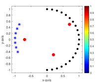
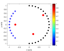
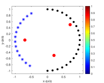
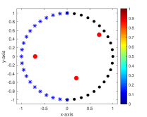
respectively. Notice that in limited-view problem, one assumes that the sets of incident and observation directions are coincide, i.e., $\mathbb{S}_{\operatorname*{inc}}=\mathbb{S}_{\operatorname*{obs}}$ because $\boldsymbol{\vartheta}_{n}=-\boldsymbol{\theta}_{n}$ for all $n=1,2,\cdots,N$. However, in the current limited-aperture problem, we assume that the sets and total number of incident and observation directions are different, i.e., $\mathbb{S}_{\operatorname*{inc}}\neq\mathbb{S}_{\operatorname*{obs}}$ and $N\neq M$. Figure 1 illustrates the comparison between the limited-aperture and limited-view inverse scattering problems. Throughout this paper, we assume that $\mathbb{S}_{\operatorname*{obs}}^{1}$ and $\mathbb{S}_{\operatorname*{inc}}^{1}$ are connected and proper subsets of $\mathbb{S}^{1}$.

$\mathbb{S}_{\operatorname*{inc}}^{1}=\mathbb{S}_{\operatorname*{obs}}^{1}$ $\Sigma_{1}$ $~{}\Sigma_{2}$ $\Sigma_{3}$ $\boldsymbol{\theta}_{n}$ $\boldsymbol{\vartheta}_{m}$
(a) Limited-view problem
$\mathbb{S}_{\operatorname*{inc}}^{1}$ $\mathbb{S}_{\operatorname*{obs}}^{1}$ $\Sigma_{1}$ $~{}\Sigma_{2}$ $\Sigma_{3}$ $\boldsymbol{\theta}_{n}$ $\boldsymbol{\vartheta}_{m}$
(b) Limited-aperture problem
Figure 1: Illustration of limited-view and limited-aperture inverse scattering problems.

As previously, let us generate an MSR matrix $\mathbb{K}\in\mathbb{C}^{M\times N}$ from $\Psi$ as

$$\mathbb{K}=\left[\begin{array}[]{cccc}u_{\infty}(\boldsymbol{\vartheta}_{1},\boldsymbol{\theta}_{1})&u_{\infty}(\boldsymbol{\vartheta}_{1},\boldsymbol{\theta}_{2})&\cdots&u_{\infty}(\boldsymbol{\vartheta}_{1},\boldsymbol{\theta}_{N})\\ u_{\infty}(\boldsymbol{\vartheta}_{2},\boldsymbol{\theta}_{1})&u_{\infty}(\boldsymbol{\vartheta}_{2},\boldsymbol{\theta}_{2})&\cdots&u_{\infty}(\boldsymbol{\vartheta}_{2},\boldsymbol{\theta}_{N})\\ \vdots&\vdots&\ddots&\vdots\\ u_{\infty}(\boldsymbol{\vartheta}_{M},\boldsymbol{\theta}_{1})&u_{\infty}(\boldsymbol{\vartheta}_{M},\boldsymbol{\theta}_{2})&\cdots&u_{\infty}(\boldsymbol{\vartheta}_{M},\boldsymbol{\theta}_{N})\\ \end{array}\right].$$

With this, we can design the MUSIC algorithm, analyze the mathematical structure of the imaging function, and explore various MUSIC properties for two different cases: dielectric permittivity contrast only ($\varepsilon(\mathbf{r})\neq\varepsilon_{\mathrm{b}}$ and $\mu(\mathbf{r})=\mu_{\mathrm{b}}$) and magnetic permeability contrast only ($\varepsilon(\mathbf{r})=\varepsilon_{\mathrm{b}}$ and $\mu(\mathbf{r})\neq\mu_{\mathrm{b}}$). Both contrast case ($\varepsilon(\mathbf{r})\neq\varepsilon_{\mathrm{b}}$ and $\mu(\mathbf{r})\neq\mu_{\mathrm{b}}$) can be derived by combining the permittivity and permeability contrast cases.

3.2 Dielectric permittivity contrast case: $\varepsilon(\mathbf{r})\neq\varepsilon_{\mathrm{b}}$ and $\mu(\mathbf{r})=\mu_{\mathrm{b}}$

First, we consider the dielectric permittivity contrast case. For the sake of simplicity, we assume that $M,N>S$ and $\varepsilon_{s}>\varepsilon_{\mathrm{b}}$ for all $s$. Then, based on the expression (7), $\mathbb{K}$ can be decomposed as

$$\mathbb{K}=\mathbb{EDF}^{T}+\mathbb{O}(\alpha^{2})\approx\mathbb{EDF}^{T},$$ (12)

where $\mathbb{O}(\alpha^{2})$ is a $M\times N$ matrix, the elements of which are $o(\alpha^{2})$, and $\mathbb{D}$ is the $S\times S$ matrix

$$\mathbb{D}=\alpha^{2}\pi\frac{k^{2}(1+i)}{4\sqrt{k\pi}}\left[\begin{array}[]{cccc}\displaystyle\frac{\varepsilon_{1}-\varepsilon_{\mathrm{b}}}{\sqrt{\varepsilon_{\mathrm{b}}\mu_{\mathrm{b}}}}&0&0&0\\ 0&\displaystyle\frac{\varepsilon_{2}-\varepsilon_{\mathrm{b}}}{\sqrt{\varepsilon_{\mathrm{b}}\mu_{\mathrm{b}}}}&0&0\\ \vdots&\vdots&\ddots&\vdots\\ 0&0&0&\displaystyle\frac{\varepsilon_{S}-\varepsilon_{\mathrm{b}}}{\sqrt{\varepsilon_{\mathrm{b}}\mu_{\mathrm{b}}}}\\ \end{array}\right]\in\mathbb{C}^{S\times S},$$

and the matrices $\mathbb{E}\in\mathbb{C}^{M\times S}$ and $\mathbb{F}\in\mathbb{C}^{N\times S}$ respectively are

$$\mathbb{E}=\left[\begin{array}[]{cccc}e^{-ik\boldsymbol{\vartheta}_{1}\cdot\mathbf{r}_{1}}&e^{-ik\boldsymbol{\vartheta}_{1}\cdot\mathbf{r}_{2}}&\cdots&e^{-ik\boldsymbol{\vartheta}_{1}\cdot\mathbf{r}_{S}}\\ e^{-ik\boldsymbol{\vartheta}_{2}\cdot\mathbf{r}_{1}}&e^{-ik\boldsymbol{\vartheta}_{2}\cdot\mathbf{r}_{2}}&\cdots&e^{-ik\boldsymbol{\vartheta}_{2}\cdot\mathbf{r}_{S}}\\ \vdots&\vdots&\ddots&\vdots\\ e^{-ik\boldsymbol{\vartheta}_{M}\cdot\mathbf{r}_{1}}&e^{-ik\boldsymbol{\vartheta}_{M}\cdot\mathbf{r}_{2}}&\cdots&e^{-ik\boldsymbol{\vartheta}_{M}\cdot\mathbf{r}_{S}}\end{array}\right]\quad\text{and}\quad\mathbb{F}=\left[\begin{array}[]{cccc}e^{ik\boldsymbol{\theta}_{1}\cdot\mathbf{r}_{1}}&e^{ik\boldsymbol{\theta}_{1}\cdot\mathbf{r}_{2}}&\cdots&e^{ik\boldsymbol{\theta}_{1}\cdot\mathbf{r}_{S}}\\ e^{ik\boldsymbol{\theta}_{2}\cdot\mathbf{r}_{1}}&e^{ik\boldsymbol{\theta}_{2}\cdot\mathbf{r}_{2}}&\cdots&e^{ik\boldsymbol{\theta}_{2}\cdot\mathbf{r}_{S}}\\ \vdots&\vdots&\ddots&\vdots\\ e^{ik\boldsymbol{\theta}_{N}\cdot\mathbf{r}_{1}}&e^{ik\boldsymbol{\theta}_{N}\cdot\mathbf{r}_{2}}&\cdots&e^{ik\boldsymbol{\theta}_{N}\cdot\mathbf{r}_{S}}\end{array}\right],$$

Let us perform SVD of $\mathbb{K}$ as

$$\mathbb{K}=\mathbb{USV}^{*}=\sum_{n=1}^{N}\sigma_{n}\mathbf{U}_{n}\mathbf{V}_{n}^{*}\approx\sum_{n=1}^{S}\sigma_{n}\mathbf{U}_{n}\mathbf{V}_{n}^{*}.$$ (13)

Then, the first $S-$columns of singular vectors $\{\mathbf{U}_{1},\mathbf{U}_{2},\cdots,\mathbf{U}_{S}\}$ and $\{\mathbf{V}_{1},\mathbf{V}_{2},\cdots,\mathbf{V}_{S}\}$ span the signal spaces of $\mathbb{KK^{*}}$ and $\mathbb{K^{*}K}$, respectively. Correspondingly, we can define orthonormal projection operators onto the noise subspaces as

$$\mathbb{P}_{\operatorname*{noise}}^{(\varepsilon)}=\mathbb{I}(S)-\sum_{s=1}^{S}\mathbf{U}_{s}\mathbf{U}_{s}^{*}\quad\text{and}\quad\mathbb{Q}_{\operatorname*{noise}}^{(\varepsilon)}=\mathbb{I}(S)-\sum_{s=1}^{S}\mathbf{V}_{s}\mathbf{V}_{s}^{*},$$

where $\mathbb{I}(S)$ denotes the $S\times S$ identity matrix.

Based on (7), we define test vectors for $\mathbf{r}\in\Omega$ as

$$\mathbf{f}_{\varepsilon}(\mathbf{r})=\frac{1}{\sqrt{M}}\bigg{[}e^{-ik\boldsymbol{\vartheta}_{1}\cdot\mathbf{r}},e^{-ik\boldsymbol{\vartheta}_{2}\cdot\mathbf{r}},\cdots,e^{-ik\boldsymbol{\vartheta}_{M}\cdot\mathbf{r}}\bigg{]}^{T}\quad\text{and}\quad\mathbf{g}_{\varepsilon}(\mathbf{r})=\frac{1}{\sqrt{N}}\bigg{[}e^{ik\boldsymbol{\theta}_{1}\cdot\mathbf{r}},e^{ik\boldsymbol{\theta}_{2}\cdot\mathbf{r}},\cdots,e^{ik\boldsymbol{\theta}_{N}\cdot\mathbf{r}}\bigg{]}^{T}.$$

Then, based on [80], it can be concluded that

$\displaystyle\mathbf{f}_{\varepsilon}(\mathbf{r})\in\operatorname*{Range}(\mathbb{KK^{*}})$ $\displaystyle\quad\text{if and only if}\quad\mathbf{r}\in\{\mathbf{r}_{1},\mathbf{r}_{2},\cdots,\mathbf{r}_{S}\}$
$\displaystyle\mathbf{g}_{\varepsilon}(\mathbf{r})\in\operatorname*{Range}(\mathbb{K^{*}K})$ $\displaystyle\quad\text{if and only if}\quad\mathbf{r}\in\{\mathbf{r}_{1},\mathbf{r}_{2},\cdots,\mathbf{r}_{S}\}$

This means that $|\mathbb{P}_{\operatorname*{noise}}^{(\varepsilon)}(\mathbf{f}_{\varepsilon}(\mathbf{r}))|=0$ and $|\mathbb{Q}_{\operatorname*{noise}}^{(\varepsilon)}(\mathbf{g}_{\varepsilon}(\mathbf{r}))|=0$ when $\mathbf{r}\in\Sigma$. Thus, the location of $\mathbf{r}_{s}\in\Sigma_{s}$ can be identified by plotting

$$f_{\operatorname*{MUSIC}}(\mathbf{r})=\frac{1}{2}\left(\frac{1}{|\mathbb{P}_{\operatorname*{noise}}^{(\varepsilon)}(\mathbf{f}_{\varepsilon}(\mathbf{r}))|}+\frac{1}{|\mathbb{Q}_{\operatorname*{noise}}^{(\varepsilon)}(\mathbf{g}_{\varepsilon}(\mathbf{r}))|}\right).$$ (14)

The resulting plot of $f_{\operatorname*{MUSIC}}(\mathbf{r})$ is expected to exhibit large-magnitude peaks (theoretically, $+\infty$) at $\mathbf{r}\in\Sigma_{s}$ for $s=1,2,\cdots,S$.

Remark 3.1 (Comparison with traditional MUSIC).

In the traditional MUSIC algorithm, $\mathbf{f}_{\varepsilon}(\mathbf{r})=\mathbf{g}_{\varepsilon}(\mathbf{r})$ and $\mathbb{P}_{\operatorname*{noise}}^{(\varepsilon)}=\mathbb{Q}_{\operatorname*{noise}}^{(\varepsilon)}$ because $\mathbb{K}$ is a complex symmetric matrix. In this case, (14) becomes (8).

To explain the feasibility of $f_{\operatorname*{MUSIC}}(\mathbf{r})$, we establish a relationship with an infinite series of integer-order Bessel functions. The derivation is given in Section A.

Theorem 3.3.

Let $\boldsymbol{\vartheta}_{m}:=[\cos\vartheta_{m},\sin\vartheta_{m}]^{T}$, $\boldsymbol{\theta}_{n}:=[\cos\theta_{n},\sin\theta_{n}]^{T}$, $\mathbf{r}:=|\mathbf{r}|[\cos\phi,\sin\phi]^{T}$, and $\mathbf{r}-\mathbf{r}_{s}:=|\mathbf{r}-\mathbf{r}_{s}|[\cos\phi_{s},\sin\phi_{s}]^{T}$. Then, for sufficiently large $k$, $f_{\operatorname*{MUSIC}}(\mathbf{r})$ can be represented as

$\displaystyle\begin{aligned} f_{\operatorname*{MUSIC}}(\mathbf{r})=&\frac{1}{2}\left(1-\sum_{s=1}^{S}\left|J_{0}(k|\mathbf{r}-\mathbf{r}_{s}|)+\frac{\Lambda_{\varepsilon}^{(1)}(\mathbf{r}-\mathbf{r}_{s})}{\vartheta_{M}-\vartheta_{1}}\right|^{2}+O\left(\frac{1}{(\vartheta_{M}-\vartheta_{1})^{2}}\right)\right)^{-1/2}\\ &+\frac{1}{2}\left(1-\sum_{s=1}^{S}\left|J_{0}(k|\mathbf{r}-\mathbf{r}_{s}|)+\frac{\Lambda_{\varepsilon}^{(2)}(\mathbf{r}-\mathbf{r}_{s})}{\theta_{N}-\theta_{1}}\right|^{2}+O\left(\frac{1}{(\theta_{N}-\theta_{1})^{2}}\right)\right)^{-1/2},\end{aligned}$ (15)

where $\Lambda_{\varepsilon}^{(1)}(\mathbf{r}-\mathbf{r}_{s})$ and $\Lambda_{\varepsilon}^{(2)}(\mathbf{r}-\mathbf{r}_{s})$ are given by (21) and (27), respectively.

Based on the identified mathematical structure of (15), the intrinsic properties of MUSIC for the dielectric permittivity contrast case can be identified.

Discussion 3.1 (Feasibility and limitation of MUSIC).

The imaging function $f_{\operatorname*{MUSIC}}(\mathbf{r})$ consists of $J_{0}(k|\mathbf{r}-\mathbf{r}_{s}|)$, $\Lambda_{\varepsilon}^{(1)}(\mathbf{r}-\mathbf{r}_{s})/(\vartheta_{M}-\vartheta_{1})$, and $\Lambda_{\varepsilon}^{(2)}(\mathbf{r}-\mathbf{r}_{s})/(\theta_{N}-\theta_{1})$. The first term is independent of the range of incident and observation directions and contributes to the detection, whereas the remaining terms are dependent on the range and disturb the detection. Since $J_{0}(0)=1$ and $J_{p}(0)=0$ for every positive integer $p$, the value of $f_{\operatorname*{MUSIC}}(\mathbf{r}_{s})$ will be sufficiently large to identify $\mathbf{r}_{s}$ via the map of $f_{\operatorname*{MUSIC}}(\mathbf{r})$. However, if $\mathbf{r}\neq\mathbf{r}_{s}$ and the range of incident or observations directions is narrow, $f_{\operatorname*{MUSIC}}(\mathbf{r})$ will be dominated by $\Lambda_{\varepsilon}^{(1)}(\mathbf{r}-\mathbf{r}_{s})/(\vartheta_{M}-\vartheta_{1})$ or $\Lambda_{\varepsilon}^{(2)}(\mathbf{r}-\mathbf{r}_{s})/(\theta_{N}-\theta_{1})$. Therefore, identifying the location of $\Sigma_{s}$ should be difficult.

Discussion 3.2 (Least range of directions).

On the basis of (15), it will be possible to obtain a good result by eliminating

$$\frac{\Lambda_{\varepsilon}^{(1)}(\mathbf{r}-\mathbf{r}_{s})}{\vartheta_{M}-\vartheta_{1}}=0\quad\text{and}\quad\frac{\Lambda_{\varepsilon}^{(2)}(\mathbf{r}-\mathbf{r}_{s})}{\theta_{N}-\theta_{1}}=0.$$

A possible choice is to select $\vartheta_{1}$, $\vartheta_{M}$, $\theta_{1}$, and $\theta_{N}$, thereby satisfying

$$\sin\frac{p(\vartheta_{M}-\vartheta_{1})}{2}\cos\frac{p(\vartheta_{M}+\vartheta_{1}-2\phi_{s}+2\pi)}{2}=0\quad\text{and}\quad\sin\frac{q(\theta_{N}-\theta_{1})}{2}\cos\frac{q(\theta_{N}+\theta_{1}-2\phi_{s})}{2}=0$$

for every positive integer $p$ and $q$. Another possible choice is the selection $\vartheta_{1}=\phi_{s}$, $\vartheta_{M}=\pi+\phi_{s}$, $\theta_{1}=\phi_{s}$, and $\theta_{N}=\pi+\phi_{s}$. Unfortunately, we do not have a priori information of $\Sigma_{s}$, this is an ideal condition, but motivated by this observation, one can obtain a good result when $\vartheta_{M}-\vartheta_{1}=\pi$ and $\theta_{N}-\theta_{1}=\pi$, i.e., if the range of incident and observation directions is wider than $\pi$, refer to Figures 4 and 6.

3.3 Magnetic permeability contrast case: $\varepsilon(\mathbf{r})=\varepsilon_{\mathrm{b}}$ and $\mu(\mathbf{r})\neq\mu_{\mathrm{b}}$

Next, we consider the magnetic permeability contrast case. Here, we assume that $M,N>2S$ and $\mu_{s}<\mu_{\mathrm{b}}$ for all $s$. Then, based on the expression (10), $\mathbb{K}$ can be decomposed as

$$\mathbb{K}=\mathbb{HBG}^{T}+\mathbb{O}(\alpha^{2})\approx\mathbb{HBG}^{T},$$ (16)

where $\mathbb{O}(\alpha^{2})$ is a $2M\times 2N$ matrix, the elements of which are $o(\alpha^{2})$, and $\mathbb{D}$ is the $2S\times 2S$ matrix

$$\mathbb{D}=\alpha^{2}\pi\frac{k^{2}(1+i)}{4\sqrt{k\pi}}\left[\begin{array}[]{cccc}\mathbb{D}_{1}&0&0&0\\ 0&\mathbb{D}_{2}&0&0\\ \vdots&\vdots&\ddots&\vdots\\ 0&0&0&\mathbb{D}_{S}\\ \end{array}\right]\in\mathbb{R}^{2S\times 2S},\quad\mathbb{D}_{s}=\left[\begin{array}[]{cc}\displaystyle\frac{\mu_{\mathrm{b}}}{\mu_{s}+\mu_{\mathrm{b}}}&0\\ 0&\displaystyle\frac{\mu_{\mathrm{b}}}{\mu_{s}+\mu_{\mathrm{b}}}\end{array}\right]$$

and the matrices $\mathbb{H}\in\mathbb{R}^{2M\times 2S}$ and $\mathbb{M}\in\mathbb{R}^{2N\times 2S}$ respectively are

$\displaystyle\mathbb{H}$ $\displaystyle=\left[\begin{array}[]{ccccccc}\mathbf{H}_{1}^{(1)}&\mathbf{H}_{1}^{(2)}&\mathbf{H}_{2}^{(1)}&\mathbf{H}_{2}^{(2)}&\cdots&\mathbf{H}_{S}^{(1)}&\mathbf{H}_{S}^{(2)}\end{array}\right]$
$\displaystyle=\left[\begin{array}[]{ccccc}(-\boldsymbol{\vartheta}_{1}\cdot\mathbf{e}_{1})e^{-ik\boldsymbol{\vartheta}_{1}\cdot\mathbf{r}_{1}}&(-\boldsymbol{\vartheta}_{1}\cdot\mathbf{e}_{2})e^{-ik\boldsymbol{\vartheta}_{1}\cdot\mathbf{r}_{1}}&\cdots&(-\boldsymbol{\vartheta}_{1}\cdot\mathbf{e}_{1})e^{-ik\boldsymbol{\vartheta}_{1}\cdot\mathbf{r}_{S}}&(-\boldsymbol{\vartheta}_{1}\cdot\mathbf{e}_{2})e^{-ik\boldsymbol{\vartheta}_{1}\cdot\mathbf{r}_{S}}\\ (-\boldsymbol{\vartheta}_{2}\cdot\mathbf{e}_{1})e^{-ik\boldsymbol{\vartheta}_{2}\cdot\mathbf{r}_{1}}&(-\boldsymbol{\vartheta}_{2}\cdot\mathbf{e}_{2})e^{-ik\boldsymbol{\vartheta}_{2}\cdot\mathbf{r}_{1}}&\cdots&(-\boldsymbol{\vartheta}_{2}\cdot\mathbf{e}_{1})e^{-ik\boldsymbol{\vartheta}_{2}\cdot\mathbf{r}_{S}}&(-\boldsymbol{\vartheta}_{2}\cdot\mathbf{e}_{2})e^{-ik\boldsymbol{\vartheta}_{2}\cdot\mathbf{r}_{S}}\\ \vdots&\vdots&\ddots&\vdots&\vdots\\ (-\boldsymbol{\vartheta}_{M}\cdot\mathbf{e}_{1})e^{-ik\boldsymbol{\vartheta}_{M}\cdot\mathbf{r}_{1}}&(-\boldsymbol{\vartheta}_{M}\cdot\mathbf{e}_{2})e^{-ik\boldsymbol{\vartheta}_{M}\cdot\mathbf{r}_{1}}&\cdots&(-\boldsymbol{\vartheta}_{M}\cdot\mathbf{e}_{1})e^{-ik\boldsymbol{\vartheta}_{M}\cdot\mathbf{r}_{S}}&(-\boldsymbol{\vartheta}_{M}\cdot\mathbf{e}_{2})e^{-ik\boldsymbol{\vartheta}_{M}\cdot\mathbf{r}_{S}}\\ \end{array}\right]$

and

$\displaystyle\mathbb{G}$ $\displaystyle=\left[\begin{array}[]{ccccccc}\mathbf{G}_{1}^{(1)}&\mathbf{G}_{1}^{(2)}&\mathbf{G}_{2}^{(1)}&\mathbf{G}_{2}^{(2)}&\cdots&\mathbf{G}_{S}^{(1)}&\mathbf{G}_{S}^{(2)}\end{array}\right]$
$\displaystyle=\left[\begin{array}[]{ccccc}(\boldsymbol{\theta}_{1}\cdot\mathbf{e}_{1})e^{-ik\boldsymbol{\vartheta}_{1}\cdot\mathbf{r}_{1}}&(\boldsymbol{\theta}_{1}\cdot\mathbf{e}_{2})e^{-ik\boldsymbol{\vartheta}_{1}\cdot\mathbf{r}_{1}}&\cdots&(\boldsymbol{\theta}_{1}\cdot\mathbf{e}_{1})e^{-ik\boldsymbol{\vartheta}_{1}\cdot\mathbf{r}_{S}}&(\boldsymbol{\theta}_{1}\cdot\mathbf{e}_{2})e^{-ik\boldsymbol{\vartheta}_{1}\cdot\mathbf{r}_{S}}\\ (\boldsymbol{\theta}_{2}\cdot\mathbf{e}_{1})e^{-ik\boldsymbol{\vartheta}_{2}\cdot\mathbf{r}_{1}}&(\boldsymbol{\theta}_{2}\cdot\mathbf{e}_{2})e^{-ik\boldsymbol{\vartheta}_{2}\cdot\mathbf{r}_{1}}&\cdots&(\boldsymbol{\theta}_{2}\cdot\mathbf{e}_{1})e^{-ik\boldsymbol{\vartheta}_{2}\cdot\mathbf{r}_{S}}&(\boldsymbol{\theta}_{2}\cdot\mathbf{e}_{2})e^{-ik\boldsymbol{\vartheta}_{2}\cdot\mathbf{r}_{S}}\\ \vdots&\vdots&\ddots&\vdots&\vdots\\ (\boldsymbol{\theta}_{N}\cdot\mathbf{e}_{1})e^{-ik\boldsymbol{\vartheta}_{N}\cdot\mathbf{r}_{1}}&(\boldsymbol{\theta}_{N}\cdot\mathbf{e}_{2})e^{-ik\boldsymbol{\vartheta}_{N}\cdot\mathbf{r}_{1}}&\cdots&(\boldsymbol{\theta}_{N}\cdot\mathbf{e}_{1})e^{-ik\boldsymbol{\vartheta}_{N}\cdot\mathbf{r}_{S}}&(\boldsymbol{\theta}_{N}\cdot\mathbf{e}_{2})e^{-ik\boldsymbol{\vartheta}_{N}\cdot\mathbf{r}_{S}}\\ \end{array}\right],$

where $\mathbf{e}_{1}=[1,0]^{T}$ and $\mathbf{e}_{2}=[0,1]^{T}$.

As in the permittivity contrast case, let us perform SVD of $\mathbb{K}$ as

$$\mathbb{K}=\mathbb{USV}^{*}=\sum_{n=1}^{N}\sigma_{n}\mathbf{U}_{n}\mathbf{V}_{n}^{*}\approx\sum_{n=1}^{2S}\sigma_{n}\mathbf{U}_{n}\mathbf{V}_{n}^{*}.$$ (17)

Then, the first $2S-$columns of singular vectors $\{\mathbf{U}_{1},\mathbf{U}_{2},\cdots,\mathbf{U}_{2S}\}$ and $\{\mathbf{V}_{1},\mathbf{V}_{2},\cdots,\mathbf{V}_{2S}\}$ span the signal spaces of $\mathbb{KK^{*}}$ and $\mathbb{K^{*}K}$, respectively. Hence, we can define orthonormal projection operators onto the noise subspaces as

$$\mathbb{P}_{\operatorname*{noise}}^{(\mu)}=\mathbb{I}(S)-\sum_{s=1}^{2S}\mathbf{U}_{s}\mathbf{U}_{s}^{*}\quad\text{and}\quad\mathbb{Q}_{\operatorname*{noise}}^{(\mu)}=\mathbb{I}(S)-\sum_{s=1}^{2S}\mathbf{V}_{s}\mathbf{V}_{s}^{*},$$

Now, on the basis of the expression (10), let us introduce the following test vectors for $\mathbf{r}\in\Omega$, $\boldsymbol{\xi}_{1},\boldsymbol{\xi}_{2}\in\mathbb{R}^{2}\backslash\{\mathbf{0}\}$,

$\displaystyle\mathbf{f}_{\mu}(\mathbf{r})$ $\displaystyle=\frac{1}{\sqrt{C_{1}}}\bigg{[}(-\boldsymbol{\vartheta}_{1}\cdot\boldsymbol{\xi}_{1})e^{-ik\boldsymbol{\vartheta}_{1}\cdot\mathbf{r}},(-\boldsymbol{\vartheta}_{2}\cdot\boldsymbol{\xi}_{1})e^{-ik\boldsymbol{\vartheta}_{2}\cdot\mathbf{r}},\cdots,(-\boldsymbol{\vartheta}_{M}\cdot\boldsymbol{\xi}_{1})e^{-ik\boldsymbol{\vartheta}_{M}\cdot\mathbf{r}}\bigg{]}^{T}$
and
$\displaystyle\mathbf{g}_{\mu}(\mathbf{r})$ $\displaystyle=\frac{1}{\sqrt{C_{2}}}\bigg{[}(\boldsymbol{\theta}_{1}\cdot\boldsymbol{\xi}_{2})e^{ik\boldsymbol{\theta}_{1}\cdot\mathbf{r}},(\boldsymbol{\theta}_{2}\cdot\boldsymbol{\xi}_{2})e^{ik\boldsymbol{\theta}_{2}\cdot\mathbf{r}},\cdots,(\boldsymbol{\theta}_{N}\cdot\boldsymbol{\xi}_{2})e^{ik\boldsymbol{\theta}_{N}\cdot\mathbf{r}}\bigg{]}^{T},$

where

$$C_{1}=\frac{\vartheta_{M}-\vartheta_{1}}{2}+\frac{1}{2}\cos(\vartheta_{M}+\vartheta_{1})\sin(\vartheta_{M}-\vartheta_{1})\quad\text{and}\quad C_{2}=\frac{\theta_{N}-\theta_{1}}{2}+\frac{1}{2}\cos(\theta_{N}+\theta_{1})\sin(\theta_{N}-\theta_{1}),$$

respectively. Based on [80], if $\boldsymbol{\xi}_{1}$ and $\boldsymbol{\xi}_{2}$ are the linear combination of $\mathbf{e}_{1}$ and $\mathbf{e}_{2}$, then we obtain

$\displaystyle\mathbf{f}_{\mu}(\mathbf{r})\in\operatorname*{Range}(\mathbb{KK^{*}})$ $\displaystyle\quad\text{if and only if}\quad\mathbf{r}\in\{\mathbf{r}_{1},\mathbf{r}_{2},\cdots,\mathbf{r}_{S}\}$
$\displaystyle\mathbf{g}_{\mu}(\mathbf{r})\in\operatorname*{Range}(\mathbb{K^{*}K})$ $\displaystyle\quad\text{if and only if}\quad\mathbf{r}\in\{\mathbf{r}_{1},\mathbf{r}_{2},\cdots,\mathbf{r}_{S}\}$

This means that $|\mathbb{P}_{\operatorname*{noise}}^{(\mu)}(\mathbf{f}_{\mu}(\mathbf{r}))|=0$ and $|\mathbb{Q}_{\operatorname*{noise}}^{(\mu)}(\mathbf{g}_{\mu}(\mathbf{r}))|=0$ when $\mathbf{r}\in\Sigma$. Thus, the location of $\mathbf{r}_{s}\in\Sigma_{s}$ can be identified by plotting

$$f_{\operatorname*{MUSIC}}(\mathbf{r})=\frac{1}{2}\left(\frac{1}{|\mathbb{P}_{\operatorname*{noise}}^{(\mu)}(\mathbf{f}_{\mu}(\mathbf{r}))|}+\frac{1}{|\mathbb{Q}_{\operatorname*{noise}}^{(\mu)}(\mathbf{g}_{\mu}(\mathbf{r}))|}\right).$$ (18)

The resulting plot of $f_{\operatorname*{MUSIC}}(\mathbf{r})$ is expected to exhibit large-magnitude peaks (theoretically, $+\infty$) at $\mathbf{r}\in\Sigma_{s}$ for $s=1,2,\cdots,S$.

Remark 3.2 (Selection of test vector).

Based on the structure of $\mathbb{H}$ and $\mathbb{M}$, $\boldsymbol{\xi}_{1}$ and $\boldsymbol{\xi}_{2}$ must be a linear combination of $\mathbf{e}_{1}$ and $\mathbf{e}_{2}$. Roughly speaking, if one has a priori information, i.e., the size of inhomogeneities is already known, the selection $\boldsymbol{\xi}_{1}=\mathbf{e}_{1}$ and $\boldsymbol{\xi}_{2}=\mathbf{e}_{2}$ will guarantee a good result. Unfortunately, since we do not have target information, estimating optimal $\boldsymbol{\xi}_{1}$ and $\boldsymbol{\xi}_{2}$ requires large computational costs; refer to [37, 38]. Hence, based on [36, 38, 63, 81], we apply the test vectors $\{\mathbf{f}_{\varepsilon}(\mathbf{r}),\mathbf{g}_{\varepsilon}(\mathbf{r})\}$ instead of $\{\mathbf{f}_{\mu}(\mathbf{r}),\mathbf{g}_{\mu}(\mathbf{r})\}$.

Now, we explore the mathematical structure of $f_{\operatorname*{MUSIC}}(\mathbf{r})$ by establishing a relationship with an infinite series of integer-order Bessel functions. The derivation is given in Section B.

Theorem 3.4.

Let $\boldsymbol{\vartheta}_{m}:=[\cos\vartheta_{m},\sin\vartheta_{m}]^{T}$, $\boldsymbol{\theta}_{n}:=[\cos\theta_{n},\sin\theta_{n}]^{T}$, $\mathbf{r}=|\mathbf{r}|[\cos\phi,\sin\phi]^{T}$, and $\mathbf{r}-\mathbf{r}_{s}:=|\mathbf{r}-\mathbf{r}_{s}|[\cos\phi_{s},\sin\phi_{s}]^{T}$. Then, for sufficiently large $k$ and test vectors $\{\mathbf{f}_{\varepsilon}(\mathbf{r}),\mathbf{g}_{\varepsilon}(\mathbf{r})\}$, $f_{\operatorname*{MUSIC}}(\mathbf{r})$ can be represented as

$\displaystyle\begin{aligned} f_{\operatorname*{MUSIC}}(\mathbf{r})=&\frac{1}{2}\left(1-\sum_{s=1}^{S}\sum_{h=1}^{2}\left|iJ_{1}(k|\mathbf{r}-\mathbf{r}_{s}|)\bigg{(}\frac{\mathbf{r}-\mathbf{r}_{s}}{|\mathbf{r}-\mathbf{r}_{s}|}\cdot\mathbf{e}_{h}\bigg{)}+\frac{\Lambda_{\mu}^{(1,h)}(\mathbf{r}-\mathbf{r}_{s})}{\vartheta_{M}-\vartheta_{1}}\right|^{2}+O\left(\frac{1}{(\vartheta_{M}-\vartheta_{1})^{2}}\right)\right)^{-1/2}\\ &+\frac{1}{2}\left(1-\sum_{s=1}^{S}\sum_{h=1}^{2}\left|iJ_{1}(k|\mathbf{r}-\mathbf{r}_{s}|)\bigg{(}\frac{\mathbf{r}-\mathbf{r}_{s}}{|\mathbf{r}-\mathbf{r}_{s}|}\cdot\mathbf{e}_{h}\bigg{)}+\frac{\Lambda_{\mu}^{(2,h)}(\mathbf{r}-\mathbf{r}_{s})}{\theta_{N}-\theta_{1}}\right|^{2}+O\left(\frac{1}{(\theta_{N}-\theta_{1})^{2}}\right)\right)^{-1/2},\end{aligned}$ (19)

where $\Lambda_{\mu}^{(1,h)}(\mathbf{r}-\mathbf{r}_{s})$ and $\Lambda_{\mu}^{(2,h)}(\mathbf{r}-\mathbf{r}_{s})$ for $h=1,2$ are given by (30), (31), (35), and (36).

Based on the identified mathematical structure of (19), we can discuss some properties of MUSIC for the magnetic permeability contrast case.

Discussion 3.3 (Feasibility and limitation of MUSIC).

The imaging function $f_{\operatorname*{MUSIC}}(\mathbf{r})$ consists of

$$iJ_{1}(k|\mathbf{r}-\mathbf{r}_{s}|)\bigg{(}\frac{\mathbf{r}-\mathbf{r}_{s}}{|\mathbf{r}-\mathbf{r}_{s}|}\cdot\mathbf{e}_{h}\bigg{)},\quad\frac{\Lambda_{\mu}^{(1,h)}(\mathbf{r}-\mathbf{r}_{s})}{\vartheta_{M}-\vartheta_{1}},\quad\text{and}\quad\frac{\Lambda_{\mu}^{(2,h)}(\mathbf{r}-\mathbf{r}_{s})}{\theta_{N}-\theta_{1}}$$

for $h=1,2$. The first term is independent of the range of incident and observation directions but does not contribute to the detection because $J_{1}(0)=0$, whereas the remaining terms are dependent. It is interesting to observe that, since $\Lambda_{\mu}^{(1,h)}(\mathbf{r}-\mathbf{r}_{s})$ and $\Lambda_{\mu}^{(2,h)}(\mathbf{r}-\mathbf{r}_{s})$ contain the factors $J_{0}(k|\mathbf{r}-\mathbf{r}_{s}|)$ and $J_{0}(0)=1$, it is possible to identify $\mathbf{r}_{s}$ via the map of $f_{\operatorname*{MUSIC}}(\mathbf{r})$ if the range of incident or observation directions is narrow. However, if $\mathbf{r}\neq\mathbf{r}_{s}$ and the range of incident or observation directions is narrow, refer to Figures 7 and 9. Otherwise, if the range is sufficiently wide, $f_{\operatorname*{MUSIC}}(\mathbf{r})$ will be dominated by the first term containing $J_{1}(k|\mathbf{r}-\mathbf{r}_{s}|)$, so that two large-magnitude peaks will appear in the neighborhood of $\mathbf{r}_{s}$; refer to Figures 8 and 10. Although this result does not yield, one cannot identify a true location with this result, based on the property of $J_{1}$.

Discussion 3.4 (Least range of directions).

Now, let us eliminate the terms that are dependent on the range of directions, i.e.,

$$\frac{\Lambda_{\mu}^{(1,h)}(\mathbf{r}-\mathbf{r}_{s})}{\vartheta_{M}-\vartheta_{1}}=0\quad\text{and}\quad\frac{\Lambda_{\mu}^{(2,h)}(\mathbf{r}-\mathbf{r}_{s})}{\theta_{N}-\theta_{1}}=0$$

for all $h=1,2$. One possible choice is to select $\vartheta_{1}$, $\vartheta_{M}$, $\theta_{1}$, and $\theta_{N}$, thereby satisfying

$$\left\{\begin{array}[]{l}\displaystyle\vskip 6.0pt plus 2.0pt minus 2.0pt\sin\frac{\vartheta_{M}-\vartheta_{1}}{2}\cos\frac{\vartheta_{M}+\vartheta_{1}}{2}=0,\quad\sin(\vartheta_{M}-\vartheta_{1})\cos(\vartheta_{M}+\vartheta_{1}-\phi_{s})=0,\\ \displaystyle\vskip 6.0pt plus 2.0pt minus 2.0pt\sin\frac{\vartheta_{M}-\vartheta_{1}}{2}\cos\frac{\vartheta_{M}+\vartheta_{1}-\phi_{s}}{2}=0,\quad\sin(\theta_{N}-\theta_{1})\cos(\theta_{N}+\theta_{1}-\phi_{s})=0,\\ \displaystyle\vskip 6.0pt plus 2.0pt minus 2.0pt\sin\frac{(1-p)(\vartheta_{M}-\vartheta_{1})}{2}\cos\frac{(1-p)(\vartheta_{M}+\vartheta_{1})+2p\phi_{s}-2p\pi}{2}=0,\\ \displaystyle\vskip 6.0pt plus 2.0pt minus 2.0pt\sin\frac{(1+n)(\vartheta_{M}-\vartheta_{1})}{2}\cos\frac{(1+p)(\vartheta_{M}+\vartheta_{1})-2p\phi_{s}+2p\pi}{2}=0,\\ \displaystyle\vskip 6.0pt plus 2.0pt minus 2.0pt\sin\frac{(1-p)(\theta_{N}-\theta_{1})}{2}\cos\frac{(1-p)(\theta_{N}+\theta_{1})+2p\phi_{s}-(2p+1)\pi}{2}=0,\\ \displaystyle\sin\frac{(1+n)(\theta_{N}-\theta_{1})}{2}\cos\frac{(1+p)(\theta_{N}+\theta_{1})-2p\phi_{s}+(2p-1)\pi}{2}=0,\end{array}\right.$$

for every positive integer $p$ and $q$. Similar to the permittivity contrast case, another possible choice is to select $\vartheta_{1}=\phi_{s}$, $\vartheta_{M}=\pi+\phi_{s}$, $\theta_{1}=\phi_{s}$, and $\theta_{N}=\pi+\phi_{s}$. Therefore, if the range of incident and observation directions is wider than $\pi$, two large-magnitude peaks will appear in the neighborhood of $\mathbf{r}_{s}$, and correspondingly, it will be possible to identify the location of $\mathbf{r}_{s}$, which is the middle point of two peaks; refer to Figures 8 and 10.

4 Simulation results

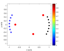
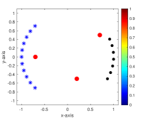
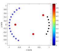
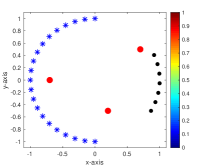
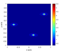
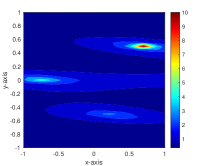
In this section, we exhibit a set of simulation results to validate the investigated results of Theorem 3.3 and Theorem 3.4. We select $S=3$ small circles with the same radii $\alpha_{s}\equiv 0.1$, permittivity $\varepsilon_{s}$, and permeability $\mu_{s}$. The locations $\mathbf{r}_{s}$ are $\mathbf{r}_{1}=[0.7,0.5]^{T}$, $\mathbf{r}_{2}=[-0.7,0.0]^{T}$, and $\mathbf{r}_{3}=[0.2,-0.5]^{T}$, and the background permittivity and permeability are $\varepsilon_{\mathrm{b}}=\mu_{\mathrm{b}}=1$. The far-field pattern data $u_{\infty}(\boldsymbol{\vartheta}_{j},\boldsymbol{\theta}_{l})$ of $\mathbb{K}$ at wavelength $k=2\pi/0.4$ are generated by solving the Foldy-Lax formulation introduced in [77] to avoid an inverse crime. After the generation of the far-field pattern, $20\text{\,}\mathrm{dB}$ white Gaussian random noise is added to the unperturbed data through the MATLAB command awgn included in the signal processing package. For incident and observation direction setting, eight different configurations are chosen, as shown in Figure 2.

Refer to caption
(a) Case 1
Refer to caption
(b) Case 2
Refer to caption
(c) Case 3
Refer to caption
(d) Case 4
Refer to caption
(e) Case 5
Refer to caption
(f) Case 6
Refer to caption
(g) Case 7
Refer to caption
(h) Case 8
Figure 2: Illustration of the configuration range. Red-colored circles denote the inhomogeneities $\Sigma_{s}$, $s=1,2,3$, and black-colored circles and blue-colored stars denote the incident and observation directions, respectively.
Example 4.1 (Permittivity contrast case: same permittivity).

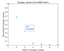
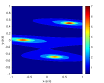
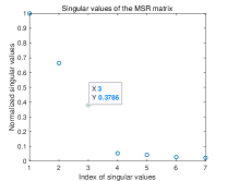
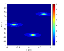
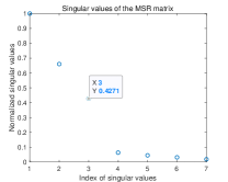
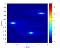
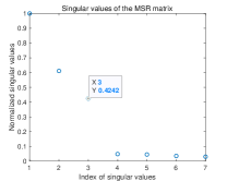
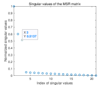
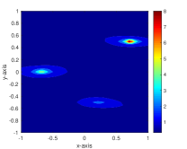
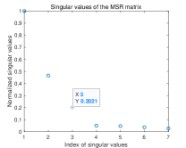
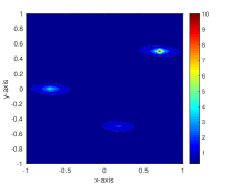
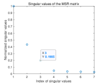
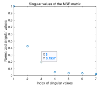
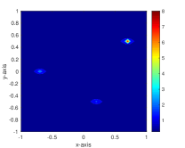
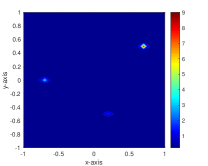
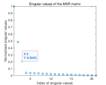
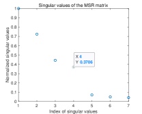
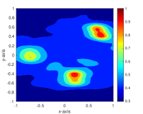
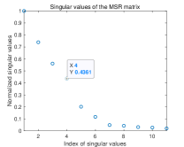
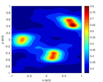
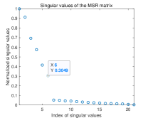
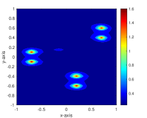
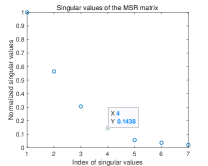
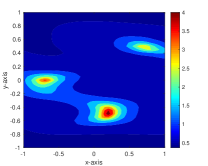
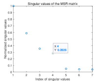
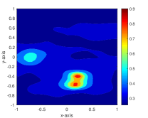
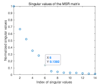
Figure 3 shows the distribution of singular values of $\mathbb{K}$ and the maps of $f_{\operatorname*{MUSIC}}(\mathbf{r})$ for Cases 1-4 when $\varepsilon_{s}\equiv 5$ and $\mu_{s}=\mu_{\mathrm{b}}$. Based on the results, we can select three singular values for generating the projection operator, and every location $\mathbf{r}_{s}$ can be identified clearly. Notice that, for Case 1, due to the appearance of the blurring effect in the neighborhood of $\mathbf{r}_{s}$, identifying the exact location of $\Sigma_{s}$ is difficult, but it is possible to recognize its existence.

Figure 4 shows the distribution of singular values of $\mathbb{K}$ and the maps of $f_{\operatorname*{MUSIC}}(\mathbf{r})$ for Cases 5-8. In contrast to the previous results, since the range of incident direction is $\pi$, the location of $\Sigma_{s}$ can be identified clearly. This result partially supports Property 3.2.

Refer to caption
Refer to caption
(a) Case 1
Refer to caption
Refer to caption
(b) Case 2
Refer to caption
Refer to caption
(c) Case 3
Refer to caption
Refer to caption
(d) Case 4
Figure 3: (Example 4.1) Distribution of singular values (first and third columns) and maps of $f_{\operatorname*{MUSIC}}(\mathbf{r})$ for $k=2\pi/0.4$ (second and fourth columns).
Refer to caption
Refer to caption
(a) Case 5
Refer to caption
Refer to caption
(b) Case 6
Refer to caption
Refer to caption
(c) Case 7
Refer to caption
Refer to caption
(d) Case 8
Figure 4: (Example 4.1) Distribution of singular values (first and third columns) and maps of $f_{\operatorname*{MUSIC}}(\mathbf{r})$ for $k=2\pi/0.4$ (second and fourth columns).
Example 4.2 (Permittivity contrast case: different permittivities).

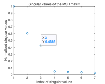
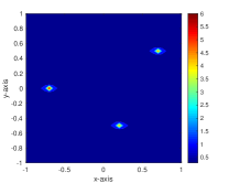
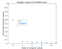
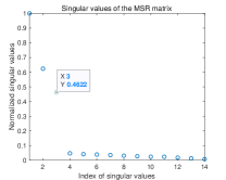
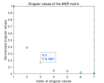
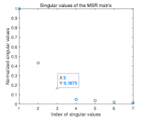
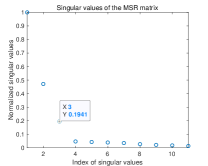
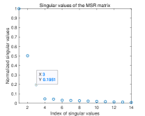
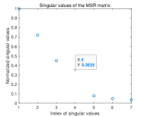
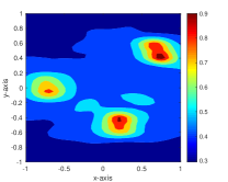
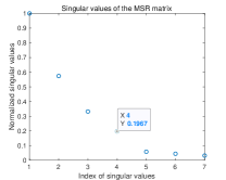
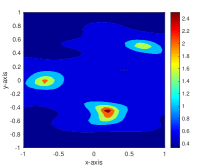
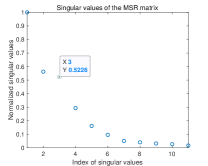
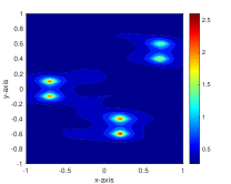
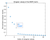
Here, we consider the imaging results for different permittivities. For this, we set $\varepsilon_{1}=5$, $\varepsilon_{2}=3$, $\varepsilon_{3}=2$, and $\mu_{s}=\mu_{\mathrm{b}}$. Figures 5 and 6 show the distribution of singular values of $\mathbb{K}$ and the maps of $f_{\operatorname*{MUSIC}}(\mathbf{r})$ for Cases 1-4. Compared with the results in Example 4.1, the selection of three nonzero singular values is more difficult. Moreover, since $\varepsilon_{3}<\varepsilon_{1},\varepsilon_{2}$, the value of $f_{\operatorname*{MUSIC}}(\mathbf{r}_{3})$ is significantly smaller than the values of $f_{\operatorname*{MUSIC}}(\mathbf{r}_{1})$ and $f_{\operatorname*{MUSIC}}(\mathbf{r}_{2})$, which means it is possible to recognize the existence of $\Sigma_{3}$, but its exact location cannot be identified.

Refer to caption
Refer to caption
(a) Case 1
Refer to caption
Refer to caption
(b) Case 2
Refer to caption
Refer to caption
(c) Case 3
Refer to caption
Refer to caption
(d) Case 4
Figure 5: (Example 4.2) Distribution of singular values (first and third columns) and maps of $f_{\operatorname*{MUSIC}}(\mathbf{r})$ for $k=2\pi/0.4$ (second and fourth columns).
Refer to caption
Refer to caption
(a) Case 5
Refer to caption
Refer to caption
(b) Case 6
Refer to caption
Refer to caption
(c) Case 7
Refer to caption
Refer to caption
(d) Case 8
Figure 6: (Example 4.2) Distribution of singular values (first and third columns) and maps of $f_{\operatorname*{MUSIC}}(\mathbf{r})$ for $k=2\pi/0.4$ (second and fourth columns).
Example 4.3 (Permeability contrast case: same permeability).

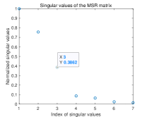
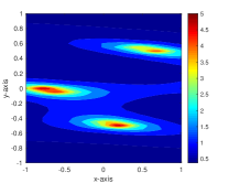
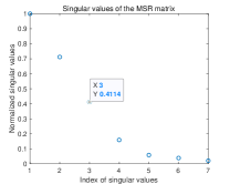
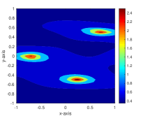
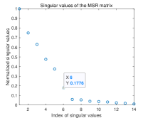
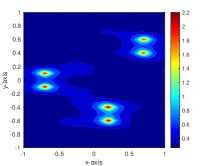
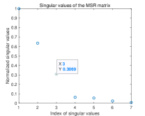
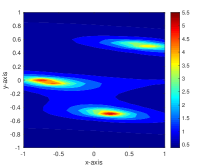
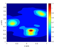
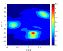
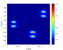
Figure 7 shows the distribution of singular values of $\mathbb{K}$ and the maps of $f_{\operatorname*{MUSIC}}(\mathbf{r})$ for Cases 1-4 when $\varepsilon_{s}=\varepsilon_{\mathrm{b}}$ and $\mu_{s}=5$. In contrast to the permittivity contrast case, only three or four singular values can be selected to generate the projection operator onto the noise subspace (theoretically, six singular values must be chosen for a proper generation). For Cases 1-3, since the range of incident and observation directions is narrower than $\pi$, the existence of $\Sigma_{s}$ can be recognized due to the factor $J_{0}(|k|\mathbf{r}-\mathbf{r}_{s}|)$ from the Discussion 3.3, but its exact location cannot be identified. For Case 4, since the range of observation direction is $\pi$, two large-magnitude peaks can be observed in the neighborhood of $\mathbf{r}_{s}$ due to the factor $J_{1}(|k|\mathbf{r}-\mathbf{r}_{s}|)$; refer to Discussion 3.4.

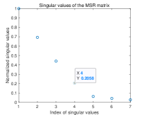
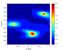
Figure 8 shows the distribution of singular values of $\mathbb{K}$ and the maps of $f_{\operatorname*{MUSIC}}(\mathbf{r})$ for Cases 5-8. Since the range of incident direction is $\pi$, two large-magnitude peaks can be observed in the neighborhood of $\mathbf{r}_{s}$. Notice that, when the range of observation direction is close to $\pi$, the two large-magnitude peaks are clearer because the value of $f_{\operatorname*{MUSIC}}(\mathbf{r})$ is dominated by $J_{1}(|k|\mathbf{r}-\mathbf{r}_{s}|)$; refer to Discussion 3.3.

Refer to caption
Refer to caption
(a) Case 1
Refer to caption
Refer to caption
(b) Case 2
Refer to caption
Refer to caption
(c) Case 3
Refer to caption
Refer to caption
(d) Case 4
Figure 7: (Example 4.3) Distribution of singular values (first and third columns) and maps of $f_{\operatorname*{MUSIC}}(\mathbf{r})$ for $k=2\pi/0.4$ (second and fourth columns).
Refer to caption
Refer to caption
(a) Case 5
Refer to caption
Refer to caption
(b) Case 6
Refer to caption
Refer to caption
(c) Case 7
Refer to caption
Refer to caption
(d) Case 8
Figure 8: (Example 4.3) Distribution of singular values (first and third columns) and maps of $f_{\operatorname*{MUSIC}}(\mathbf{r})$ for $k=2\pi/0.4$ (second and fourth columns).
Example 4.4 (Permeability contrast case: different permeabilities).

For the final simulation, we consider the imaging results with different permeabilities. For this, we set $\mu_{1}=5$, $\mu_{2}=3$, $\mu_{3}=2$, and $\varepsilon_{s}=\varepsilon_{\mathrm{b}}$. In contrast to the permittivity contrast case in Example 4.2, since the far-field pattern data are influenced by the inverse proportion of $\mu_{s}$, the location of $\mathbf{r}_{3}$ can be easily identified, but $\mathbf{r}_{1}$ cannot. It is interesting to observe that, for Case 6, three singular values can be selected to generate the projection operator onto the noise subspace, which means that some inhomogeneities (here, $\Sigma_{1}$) cannot be recognized via MUSIC. Hence, the development of an effective technique for selecting nonzero singular values must be considered at the beginning of the imaging procedure.

Refer to caption
Refer to caption
(a) Case 1
Refer to caption
Refer to caption
(b) Case 2
Refer to caption
Refer to caption
(c) Case 3
Refer to caption
Refer to caption
(d) Case 4
Figure 9: (Example 4.4) Distribution of singular values (first and third columns) and maps of $f_{\operatorname*{MUSIC}}(\mathbf{r})$ for $k=2\pi/0.4$ (second and fourth columns).
Refer to caption
Refer to caption
(a) Case 5
Refer to caption
Refer to caption
(b) Case 6
Refer to caption
Refer to caption
(c) Case 7
Refer to caption
Refer to caption
(d) Case 8
Figure 10: (Example 4.4) Distribution of singular values (first and third columns) and maps of $f_{\operatorname*{MUSIC}}(\mathbf{r})$ for $k=2\pi/0.4$ (second and fourth columns).

5 Concluding remarks

In this paper, we designed a MUSIC-type imaging technique to identify the location of small inhomogeneities, the permittivity or permeability of which differs from the background. To explain the applicability of MUSIC in the limited-aperture problem, the mathematical structure of the imaging function was derived by establishing a relationship with an infinite series of first-kind integer-order Bessel functions and the range of incident and observation directions. Based on the explored structure, we examined the various properties of MUSIC and least condition of the range of incident and observation directions to guarantee good results. Various simulation results with noisy data were conducted to validate the theoretical results.

Unfortunately, on the basis of the theoretical and simulation results, it is hard to say that the imaging results via MUSIC do not guarantee complete location identification of the inhomogeneities (especially for the magnetic permeability contrast case). Therefore, improvement of the imaging/detection performance is an interesting research subject that should be examined.

It has been confirmed that MUSIC is an effective non-iterative imaging technique in real-world microwave imaging; refer to [53]. Application to real-world microwave imaging with a limited-aperture measurement configuration will be a forthcoming work. Finally, the design of the imaging algorithm, the analysis of mathematical structure, and the numerical simulations conducted in this paper could be extended to the three-dimensional limited-aperture inverse scattering problem.

Acknowledgment

The author would like to acknowledge two anonymous referees for their comments that help to increase the quality of the paper. This research was supported by the National Research Foundation of Korea (NRF) grant funded by the Korean government (MSIT) (NRF-2020R1A2C1A01005221).

Appendix A Derivation of Theorem 3.3

On the basis of (12) and (13), the following relationship holds

$$\mathbf{U}_{s}\approx e^{i\gamma_{s}^{(1)}}\mathbf{f}_{\varepsilon}(\mathbf{r}_{s}),\quad\mathbf{V}_{s}\approx e^{-i\gamma_{s}^{(2)}}\overline{\mathbf{g}}_{\varepsilon}(\mathbf{r}_{s}),\quad\text{and}\quad\gamma_{s}^{(1)}+\gamma_{s}^{(2)}=\arg\left(\frac{\alpha^{2}k^{2}(1+i)(\varepsilon_{s}-\varepsilon_{\mathrm{b}})\pi}{4\sqrt{MNk\varepsilon_{\mathrm{b}}\mu_{\mathrm{b}}\pi}}\right),$$

With this, we can evaluate

$\displaystyle\mathbb{P}_{\operatorname*{noise}}^{(\varepsilon)}(\mathbf{f}_{\varepsilon}(\mathbf{r}))$ $\displaystyle=\left(\mathbb{I}(S)-\sum_{s=1}^{S}\mathbf{U}_{s}\mathbf{U}_{s}^{*}\right)\mathbf{f}_{\varepsilon}(\mathbf{r})=\left(\mathbb{I}(S)-\frac{1}{M}\sum_{s=1}^{S}\mathbf{f}_{\varepsilon}(\mathbf{r}_{s})\mathbf{f}_{\varepsilon}(\mathbf{r}_{s})^{*}\right)\mathbf{f}_{\varepsilon}(\mathbf{r})$
$\displaystyle=\frac{1}{\sqrt{M}}\left[\begin{array}[]{c}e^{-ik\boldsymbol{\vartheta}_{1}\cdot\mathbf{r}}\\ e^{-ik\boldsymbol{\vartheta}_{2}\cdot\mathbf{r}}\\ \vdots\\ e^{-ik\boldsymbol{\vartheta}_{M}\cdot\mathbf{r}}\end{array}\right]-\frac{1}{M\sqrt{M}}\sum_{s=1}^{S}\left[\begin{array}[]{c}\vskip 6.0pt plus 2.0pt minus 2.0pt\displaystyle e^{-ik\boldsymbol{\vartheta}_{1}\cdot\mathbf{r}}+\sum_{m\in\mathcal{M}_{1}}e^{-ik\boldsymbol{\vartheta}_{1}\cdot\mathbf{r}_{s}}e^{-ik\boldsymbol{\vartheta}_{m}\cdot(\mathbf{r}-\mathbf{r}_{s})}\\ \vskip 6.0pt plus 2.0pt minus 2.0pt\displaystyle e^{-ik\boldsymbol{\vartheta}_{2}\cdot\mathbf{r}}+\sum_{m\in\mathcal{M}_{2}}e^{-ik\boldsymbol{\vartheta}_{2}\cdot\mathbf{r}_{s}}e^{-ik\boldsymbol{\vartheta}_{m}\cdot(\mathbf{r}-\mathbf{r}_{s})}\\ \vskip 6.0pt plus 2.0pt minus 2.0pt\vdots\\ \vskip 6.0pt plus 2.0pt minus 2.0pt\displaystyle e^{-ik\boldsymbol{\vartheta}_{M}\cdot\mathbf{r}}+\sum_{m\in\mathcal{M}_{M}}e^{-ik\boldsymbol{\vartheta}_{M}\cdot\mathbf{r}_{s}}e^{-ik\boldsymbol{\vartheta}_{m}\cdot(\mathbf{r}-\mathbf{r}_{s})}\\ \end{array}\right],$

where $\mathcal{M}_{p}=\{1,2,\cdots,M\}\backslash\{p\}$. Since $e^{-ik\boldsymbol{\vartheta}_{p}\cdot\mathbf{r}}=e^{-ik\boldsymbol{\vartheta}_{p}\cdot\mathbf{r}_{s}}e^{-ik\boldsymbol{\vartheta}_{p}\cdot(\mathbf{r}-\mathbf{r}_{s})}$ and the following relation

$\displaystyle\begin{aligned} \frac{1}{M}\sum_{m=1}^{M}e^{-ik\boldsymbol{\vartheta}_{m}\cdot\mathbf{r}}&=\frac{1}{\vartheta_{M}-\vartheta_{1}}\int_{\mathbb{S}_{\operatorname*{obs}}^{1}}e^{-ik\boldsymbol{\vartheta}\cdot\mathbf{r}}d\boldsymbol{\vartheta}\\ &=J_{0}(k|\mathbf{r}|)+\frac{4}{\vartheta_{M}-\vartheta_{1}}\sum_{p=1}^{\infty}\frac{i^{p}}{p}J_{p}(k|\mathbf{r}|)\sin\frac{p(\vartheta_{M}-\vartheta_{1})}{2}\cos\frac{p(\vartheta_{M}+\vartheta_{1}-2\phi+2\pi)}{2},\end{aligned}$ (20)

holds uniformly (see [81], for instance), we can derive

$\displaystyle\frac{1}{M}\sum_{s=1}^{S}\left(e^{-ik\boldsymbol{\vartheta}_{p}\cdot\mathbf{r}}+\sum_{p\in\mathcal{M}_{p}}e^{-ik\boldsymbol{\vartheta}_{p}\cdot\mathbf{r}_{s}}e^{-ik\boldsymbol{\vartheta}_{p}\cdot(\mathbf{r}-\mathbf{r}_{s})}\right)=\sum_{s=1}^{S}e^{-ik\boldsymbol{\vartheta}_{p}\cdot\mathbf{r}_{s}}\left(\frac{1}{M}\sum_{m=1}^{M}e^{-ik\boldsymbol{\vartheta}_{m}\cdot(\mathbf{r}-\mathbf{r}_{s})}\right)$
$\displaystyle=\sum_{s=1}^{S}e^{-ik\boldsymbol{\vartheta}_{p}\cdot\mathbf{r}_{s}}\left(J_{0}(k|\mathbf{r}-\mathbf{r}_{s}|)+\frac{4}{\vartheta_{M}-\vartheta_{1}}\sum_{p=1}^{\infty}\frac{i^{p}}{p}J_{p}(k|\mathbf{r}-\mathbf{r}_{s}|)\sin\frac{p(\vartheta_{M}-\vartheta_{1})}{2}\cos\frac{p(\vartheta_{M}+\vartheta_{1}-2\phi_{s}+2\pi)}{2}\right).$

Now, let us denote

$$\Lambda_{\varepsilon}^{(1)}(\mathbf{r}-\mathbf{r}_{s}):=4\sum_{p=1}^{\infty}\frac{i^{p}}{p}J_{p}(k|\mathbf{r}-\mathbf{r}_{s}|)\sin\frac{p(\vartheta_{M}-\vartheta_{1})}{2}\cos\frac{p(\vartheta_{M}+\vartheta_{1}-2\phi_{s}+2\pi)}{2}.$$ (21)

As such, we obtain

$$\mathbb{P}_{\operatorname*{noise}}^{(\varepsilon)}(\mathbf{f}_{\varepsilon}(\mathbf{r}))=\frac{1}{\sqrt{M}}\left[\begin{array}[]{c}\vskip 6.0pt plus 2.0pt minus 2.0pt\displaystyle e^{-ik\boldsymbol{\vartheta}_{1}\cdot\mathbf{r}}-\sum_{s=1}^{S}e^{-ik\boldsymbol{\vartheta}_{1}\cdot\mathbf{r}_{s}}\left(J_{0}(k|\mathbf{r}-\mathbf{r}_{s}|)+\frac{\Lambda_{\varepsilon}^{(1)}(\mathbf{r}-\mathbf{r}_{s})}{\vartheta_{M}-\vartheta_{1}}\right)\\ \vskip 6.0pt plus 2.0pt minus 2.0pt\displaystyle e^{-ik\boldsymbol{\vartheta}_{2}\cdot\mathbf{r}}-\sum_{s=1}^{S}e^{-ik\boldsymbol{\vartheta}_{2}\cdot\mathbf{r}_{s}}\left(J_{0}(k|\mathbf{r}-\mathbf{r}_{s}|)+\frac{\Lambda_{\varepsilon}^{(1)}(\mathbf{r}-\mathbf{r}_{s})}{\vartheta_{M}-\vartheta_{1}}\right)\\ \vskip 6.0pt plus 2.0pt minus 2.0pt\vdots\\ \displaystyle e^{-ik\boldsymbol{\vartheta}_{M}\cdot\mathbf{r}}-\sum_{s=1}^{S}e^{-ik\boldsymbol{\vartheta}_{M}\cdot\mathbf{r}_{s}}\left(J_{0}(k|\mathbf{r}-\mathbf{r}_{s}|)+\frac{\Lambda_{\varepsilon}^{(1)}(\mathbf{r}-\mathbf{r}_{s})}{\vartheta_{M}-\vartheta_{1}}\right)\end{array}\right].$$

Now, let us denote

$$\Phi_{\varepsilon}(\mathbf{r}-\mathbf{r}_{s})=J_{0}(k|\mathbf{r}-\mathbf{r}_{s}|)+\frac{\Lambda_{\varepsilon}^{(1)}(\mathbf{r}-\mathbf{r}_{s})}{\vartheta_{M}-\vartheta_{1}}$$

by which we obtain

$$\mathbb{P}_{\operatorname*{noise}}^{(\varepsilon)}(\mathbf{f}_{\varepsilon}(\mathbf{r}))\cdot\overline{\mathbb{P}_{\operatorname*{noise}}^{(\varepsilon)}(\mathbf{f}_{\varepsilon}(\mathbf{r}))}=\frac{1}{M}\sum_{m=1}^{M}\left(1-\sum_{s=1}^{S}\Big{(}\Phi_{\varepsilon}(\mathbf{r}-\mathbf{r}_{s})e^{-ik\boldsymbol{\vartheta}_{m}\cdot(\mathbf{r}_{s}-\mathbf{r})}+\overline{\Phi_{\varepsilon}(\mathbf{r}-\mathbf{r}_{s})}e^{ik\boldsymbol{\vartheta}_{m}\cdot(\mathbf{r}-\mathbf{r}_{s})}\Big{)}\right.\\ \left.+\sum_{s=1}^{S}\sum_{s^{\prime}=1}^{S}\Phi_{\varepsilon}(\mathbf{r}-\mathbf{r}_{s})\overline{\Phi_{\varepsilon}(\mathbf{r}_{s^{\prime}}-\mathbf{r})}e^{-ik\boldsymbol{\vartheta}_{m}\cdot(\mathbf{r}_{s}-\mathbf{r}_{s^{\prime}})}\right).$$

Applying (20), we can evaluate

$\displaystyle\begin{aligned} &\frac{1}{M}\sum_{m=1}^{M}\sum_{s=1}^{S}\Phi_{\varepsilon}(\mathbf{r}-\mathbf{r}_{s})e^{-ik\boldsymbol{\vartheta}_{m}\cdot(\mathbf{r}-\mathbf{r}_{s})}=\sum_{s=1}^{S}\Phi_{\varepsilon}(\mathbf{r}-\mathbf{r}_{s})\overline{\Phi_{\varepsilon}(\mathbf{r}-\mathbf{r}_{s})}\\ &\frac{1}{M}\sum_{m=1}^{M}\sum_{s=1}^{S}\overline{\Phi_{\varepsilon}(\mathbf{r}-\mathbf{r}_{s})}e^{ik\boldsymbol{\vartheta}_{m}\cdot(\mathbf{r}-\mathbf{r}_{s})}=\sum_{s=1}^{S}\overline{\Phi_{\varepsilon}(\mathbf{r}-\mathbf{r}_{s})}\Phi_{\varepsilon}(\mathbf{r}-\mathbf{r}_{s}).\end{aligned}$ (22)

Now, let us assume that $s\neq s^{\prime}$ and $\mathbf{r}_{s}-\mathbf{r}_{s^{\prime}}=|\mathbf{r}_{s}-\mathbf{r}_{s^{\prime}}|[\cos\xi,\sin\xi]^{T}$. Then we obtain

$$\frac{1}{M}\sum_{m=1}^{M}e^{-ik\boldsymbol{\vartheta}_{m}\cdot(\mathbf{r}_{s}-\mathbf{r}_{s^{\prime}})}=J_{0}(k|\mathbf{r}_{s}-\mathbf{r}_{s^{\prime}}|)\\ +\frac{4}{\vartheta_{M}-\vartheta_{1}}\sum_{p=1}^{\infty}\frac{i^{p}}{p}J_{p}(k|\mathbf{r}_{s}-\mathbf{r}_{s^{\prime}}|)\sin\frac{p(\vartheta_{M}-\vartheta_{1})}{2}\cos\frac{p(\vartheta_{M}+\vartheta_{1}-2\xi+2\pi)}{2}.$$

Since $k$ satisfies (1), the following asymptotic form of Bessel function holds

$$J_{0}(k|\mathbf{r}_{s}-\mathbf{r}_{s^{\prime}}|)=\sqrt{\frac{2}{k\pi|\mathbf{r}_{s}-\mathbf{r}_{s^{\prime}}|}}\cos\left(k|\mathbf{r}_{s}-\mathbf{r}_{s^{\prime}}|)-\frac{\pi}{4}\right).$$ (23)

Furthermore, since for $p>0$ and $x\neq 0$ (see [82]), it can be expressed as

$$|J_{p}(x)|\leq\sup\left\{\frac{b}{\sqrt[3]{p}},\frac{c}{\sqrt[3]{|x|}}:b=0.674885\ldots,~{}c=0.785747\ldots\right\},$$ (24)

We can also observe that, for $s\neq s^{\prime}$,

$$\sum_{s=1}^{S}\sum_{s^{\prime}=1}^{S}\Phi_{\varepsilon}(\mathbf{r}-\mathbf{r}_{s})\overline{\Phi_{\varepsilon}(\mathbf{r}_{s^{\prime}}-\mathbf{r})}e^{-ik\boldsymbol{\vartheta}_{m}\cdot(\mathbf{r}_{s}-\mathbf{r}_{s^{\prime}})}=O\left(\frac{1}{(\vartheta_{M}-\vartheta_{1})^{2}}\right).$$ (25)

If $s=s^{\prime}$, then $e^{-ik\boldsymbol{\vartheta}_{m}\cdot(\mathbf{r}_{s}-\mathbf{r}_{s^{\prime}})}=1$, and, on the basis of (25), we can examine that

$$\sum_{s=1}^{S}\sum_{s^{\prime}=1}^{S}\Phi_{\varepsilon}(\mathbf{r}-\mathbf{r}_{s})\overline{\Phi_{\varepsilon}(\mathbf{r}_{s^{\prime}}-\mathbf{r})}e^{-ik\boldsymbol{\vartheta}_{m}\cdot(\mathbf{r}_{s}-\mathbf{r}_{s^{\prime}})}=\sum_{s=1}^{S}\Phi_{\varepsilon}(\mathbf{r}-\mathbf{r}_{s})\overline{\Phi_{\varepsilon}(\mathbf{r}-\mathbf{r}_{s})}=O\left(\frac{1}{(\vartheta_{M}-\vartheta_{1})^{2}}\right).$$ (26)

Finally, by combining (LABEL:Term1) and (26), we obtain

$\displaystyle\mathbb{P}_{\operatorname*{noise}}^{(\varepsilon)}(\mathbf{f}_{\varepsilon}(\mathbf{r}))\cdot\overline{\mathbb{P}_{\operatorname*{noise}}^{(\varepsilon)}(\mathbf{f}_{\varepsilon}(\mathbf{r}))}$ $\displaystyle=1-\sum_{s=1}^{S}\Phi_{\varepsilon}(\mathbf{r}-\mathbf{r}_{s})\overline{\Phi_{\varepsilon}(\mathbf{r}-\mathbf{r}_{s})}+O\left(\frac{1}{(\vartheta_{M}-\vartheta_{1})^{2}}\right)$
$\displaystyle=1-\sum_{s=1}^{S}\left|J_{0}(k|\mathbf{r}-\mathbf{r}_{s}|)+\frac{\Lambda_{\varepsilon}^{(1)}(\mathbf{r}-\mathbf{r}_{s})}{\vartheta_{M}-\vartheta_{1}}\right|^{2}+O\left(\frac{1}{(\vartheta_{M}-\vartheta_{1})^{2}}\right).$

Similarly, by letting

$$\Lambda_{\varepsilon}^{(2)}(\mathbf{r}-\mathbf{r}_{s}):=4\sum_{q=1}^{\infty}\frac{i^{q}}{q}J_{q}(k|\mathbf{r}-\mathbf{r}_{s}|)\sin\frac{q(\theta_{N}-\theta_{1})}{2}\cos\frac{q(\theta_{N}+\theta_{1}-2\phi_{s})}{2},$$ (27)

we can obtain

$$\mathbb{Q}_{\operatorname*{noise}}^{(\varepsilon)}(\mathbf{g}_{\varepsilon}(\mathbf{r}))\cdot\overline{\mathbb{Q}_{\operatorname*{noise}}^{(\varepsilon)}(\mathbf{g}_{\varepsilon}(\mathbf{r}))}=1-\sum_{s=1}^{S}\left|J_{0}(k|\mathbf{r}-\mathbf{r}_{s}|)+\frac{\Lambda_{\varepsilon}^{(2)}(\mathbf{r}-\mathbf{r}_{s})}{\theta_{N}-\theta_{1}}\right|^{2}+O\left(\frac{1}{(\theta_{N}-\theta_{1})^{2}}\right).$$

Hence, (15) is derived. This completes the proof.

Appendix B Derivation of Theorem 3.4

On the basis of (16) and (17), the following relationship holds

$\displaystyle\mathbf{U}_{2s-1}\approx e^{i\gamma_{s}^{(1,1)}}\mathbf{H}_{s}^{(1)}(\mathbf{r}_{s}),\quad\mathbf{U}_{2s}\approx e^{i\gamma_{s}^{(1,2)}}\mathbf{H}_{s}^{(2)}(\mathbf{r}_{s}),\quad\mathbf{V}_{2s-1}\approx e^{-i\gamma_{s}^{(2,1)}}\mathbf{G}_{s}^{(1)}(\mathbf{r}_{s}),\quad\mathbf{V}_{2s}\approx e^{-i\gamma_{s}^{(2,2)}}\mathbf{G}_{s}^{(2)}(\mathbf{r}_{s})$

and

$$\gamma_{s}^{(1,1)}+\gamma_{s}^{(2,1)}=\gamma_{s}^{(1,2)}+\gamma_{s}^{(2,2)}=\arg\left(\frac{\alpha^{2}k^{2}(1+i)\mu_{\mathrm{b}}\pi}{2(\mu_{s}+\mu_{\mathrm{b}})\sqrt{MNk\pi}}\right).$$

With this, we can evaluate

$\displaystyle\mathbb{P}_{\operatorname*{noise}}^{(\mu)}(\mathbf{f}_{\varepsilon}(\mathbf{r}))$ $\displaystyle=\left(\mathbb{I}(S)-\sum_{s=1}^{2S}\mathbf{U}_{s}\mathbf{U}_{s}^{*}\right)\mathbf{f}_{\varepsilon}(\mathbf{r})=\left(\mathbb{I}(S)-\frac{1}{C_{1}}\sum_{s=1}^{S}\Big{(}\mathbf{H}_{s}^{(1)}(\mathbf{r}_{s})\mathbf{H}_{s}^{(1)}(\mathbf{r}_{s})^{*}+\mathbf{H}_{s}^{(2)}(\mathbf{r}_{s})\mathbf{H}_{s}^{(2)}(\mathbf{r}_{s})^{*}\Big{)}\right)\mathbf{f}_{\varepsilon}(\mathbf{r})$
$\displaystyle=\frac{1}{\sqrt{M}}\left[\begin{array}[]{c}e^{-ik\boldsymbol{\vartheta}_{1}\cdot\mathbf{r}}\\ e^{-ik\boldsymbol{\vartheta}_{2}\cdot\mathbf{r}}\\ \vdots\\ e^{-ik\boldsymbol{\vartheta}_{M}\cdot\mathbf{r}}\end{array}\right]-\frac{1}{C_{1}\sqrt{M}}\sum_{s=1}^{S}\left[\begin{array}[]{c}K_{1}\\ K_{2}\\ \vdots\\ K_{M}\end{array}\right],$

where

$\displaystyle K_{m}=$ $\displaystyle(-\boldsymbol{\vartheta}_{m}\cdot\mathbf{e}_{1})^{2}e^{-ik\boldsymbol{\vartheta}_{m}\cdot\mathbf{r}}+(-\boldsymbol{\vartheta}_{m}\cdot\mathbf{e}_{1})e^{-ik\boldsymbol{\vartheta}_{m}\cdot\mathbf{r}_{s}}\sum_{p\in\mathcal{M}_{m}}(-\boldsymbol{\vartheta}_{p}\cdot\mathbf{e}_{1})e^{-ik\boldsymbol{\vartheta}_{p}\cdot(\mathbf{r}-\mathbf{r}_{s})}$
$\displaystyle+(-\boldsymbol{\vartheta}_{m}\cdot\mathbf{e}_{2})^{2}e^{-ik\boldsymbol{\vartheta}_{m}\cdot\mathbf{r}}+(-\boldsymbol{\vartheta}_{m}\cdot\mathbf{e}_{2})e^{-ik\boldsymbol{\vartheta}_{m}\cdot\mathbf{r}_{s}}\sum_{p\in\mathcal{M}_{m}}(-\boldsymbol{\vartheta}_{p}\cdot\mathbf{e}_{2})e^{-ik\boldsymbol{\vartheta}_{p}\cdot(\mathbf{r}-\mathbf{r}_{s})}$

for $m=1,2,\cdots,M$. Since $e^{-ik\boldsymbol{\vartheta}_{m}\cdot\mathbf{r}}=e^{-ik\boldsymbol{\vartheta}_{m}\cdot\mathbf{r}_{s}}e^{-ik\boldsymbol{\vartheta}_{m}\cdot(\mathbf{r}-\mathbf{r}_{s})}$, the following relations hold uniformly (see [81] for instance)

$\displaystyle\begin{aligned} \int_{\mathbb{S}_{\operatorname*{obs}}^{1}}(-\boldsymbol{\vartheta}\cdot\mathbf{e}_{1})&e^{-ik\boldsymbol{\vartheta}\cdot\mathbf{r}}d\boldsymbol{\vartheta}=2J_{0}(k|\mathbf{r}|)\sin\frac{\vartheta_{M}-\vartheta_{1}}{2}\cos\frac{\vartheta_{M}+\vartheta_{1}}{2}\\ &+iJ_{1}(k|\mathbf{r}|)\bigg{[}(\vartheta_{M}-\vartheta_{1})\bigg{(}\frac{\mathbf{r}}{|\mathbf{r}|}\cdot\mathbf{e}_{1}\bigg{)}+\sin(\vartheta_{M}-\vartheta_{1})\cos(\vartheta_{M}+\vartheta_{1}-\phi)\bigg{]}\\ &+2\sum_{p=2}^{\infty}i^{p}J_{p}(k|\mathbf{r}|)\bigg{[}\frac{1}{1-p}\sin\frac{(1-p)(\vartheta_{M}-\vartheta_{1})}{2}\cos\frac{(1-p)(\vartheta_{M}+\vartheta_{1})+2p\phi-2p\pi}{2}\\ &+\frac{1}{1+p}\sin\frac{(1+n)(\vartheta_{M}-\vartheta_{1})}{2}\cos\frac{(1+p)(\vartheta_{M}+\vartheta_{1})-2p\phi+2p\pi}{2}\bigg{]}\end{aligned}$ (28)

and

$\displaystyle\begin{aligned} \int_{\mathbb{S}_{\operatorname*{obs}}^{1}}(-\boldsymbol{\vartheta}\cdot\mathbf{e}_{2})&e^{-ik\boldsymbol{\vartheta}\cdot\mathbf{r}}d\boldsymbol{\vartheta}=2J_{0}(k|\mathbf{r}|)\sin\frac{\vartheta_{M}-\vartheta_{1}}{2}\cos\frac{\vartheta_{M}+\vartheta_{1}-\pi}{2}\\ &+iJ_{1}(k|\mathbf{r}|)\bigg{[}(\vartheta_{M}-\vartheta_{1})\bigg{(}\frac{\mathbf{r}}{|\mathbf{r}|}\cdot\mathbf{e}_{2}\bigg{)}+\sin(\vartheta_{M}-\vartheta_{1})\sin(\vartheta_{M}+\vartheta_{1}-\phi)\bigg{]}\\ &+2\sum_{p=2}^{\infty}i^{p}J_{p}(k|\mathbf{r}|)\bigg{[}\frac{1}{1-p}\sin\frac{(1-p)(\vartheta_{M}-\vartheta_{1})}{2}\cos\frac{(1-p)(\vartheta_{M}+\vartheta_{1})+2p\phi-(2p+1)\pi}{2}\\ &+\frac{1}{1+p}\sin\frac{(1+n)(\vartheta_{M}-\vartheta_{1})}{2}\cos\frac{(1+p)(\vartheta_{M}+\vartheta_{1})-2p\phi+(2p-1)\pi}{2}\bigg{]},\end{aligned}$ (29)

we can derive

$\displaystyle\frac{1}{C_{1}}K_{m}=$ $\displaystyle(-\boldsymbol{\vartheta}_{m}\cdot\mathbf{e}_{1})e^{-ik\boldsymbol{\vartheta}_{m}\cdot\mathbf{r}_{s}}\frac{1}{C_{1}}\sum_{m^{\prime}=1}^{M}(\boldsymbol{\vartheta}_{m^{\prime}}\cdot\mathbf{e}_{1})e^{-ik\boldsymbol{\vartheta}_{m^{\prime}}\cdot(\mathbf{r}-\mathbf{r}_{s})}$
$\displaystyle+(-\boldsymbol{\vartheta}_{m}\cdot\mathbf{e}_{2})e^{-ik\boldsymbol{\vartheta}_{m}\cdot\mathbf{r}_{s}}\frac{1}{C_{1}}\sum_{m^{\prime}=1}^{M}(\boldsymbol{\vartheta}_{m^{\prime}}\cdot\mathbf{e}_{2})e^{-ik\boldsymbol{\vartheta}_{m^{\prime}}\cdot(\mathbf{r}-\mathbf{r}_{s})}$
$\displaystyle=$ $\displaystyle(-\boldsymbol{\vartheta}_{m}\cdot\mathbf{e}_{1})e^{-ik\boldsymbol{\vartheta}_{m}\cdot\mathbf{r}_{s}}\left\{iJ_{1}(k|\mathbf{r}-\mathbf{r}_{s}|)\bigg{(}\frac{\mathbf{r}-\mathbf{r}_{s}}{|\mathbf{r}-\mathbf{r}_{s}|}\cdot\mathbf{e}_{1}\bigg{)}+\frac{\Lambda_{\mu}^{(1,1)}(\mathbf{r}-\mathbf{r}_{s})}{\vartheta_{M}-\vartheta_{1}}\right\}$
$\displaystyle+(-\boldsymbol{\vartheta}_{m}\cdot\mathbf{e}_{2})e^{-ik\boldsymbol{\vartheta}_{m}\cdot\mathbf{r}_{s}}\left\{iJ_{1}(k|\mathbf{r}-\mathbf{r}_{s}|)\bigg{(}\frac{\mathbf{r}-\mathbf{r}_{s}}{|\mathbf{r}-\mathbf{r}_{s}|}\cdot\mathbf{e}_{2}\bigg{)}+\frac{\Lambda_{\mu}^{(1,2)}(\mathbf{r}-\mathbf{r}_{s})}{\vartheta_{M}-\vartheta_{1}}\right\},$

where

$\displaystyle\begin{aligned} \Lambda_{\mu}^{(1,1)}(\mathbf{r}-\mathbf{r}_{s}):=&2J_{0}(k|\mathbf{r}-\mathbf{r}_{s}|)\sin\frac{\vartheta_{M}-\vartheta_{1}}{2}\cos\frac{\vartheta_{M}+\vartheta_{1}}{2}+iJ_{1}(k|\mathbf{r}-\mathbf{r}_{s}|)\sin(\vartheta_{M}-\vartheta_{1})\cos(\vartheta_{M}+\vartheta_{1}-\phi_{s})\\ &+2\sum_{p=2}^{\infty}i^{p}J_{p}(k|\mathbf{r}-\mathbf{r}_{s}|)\bigg{[}\frac{1}{1-p}\sin\frac{(1-p)(\vartheta_{M}-\vartheta_{1})}{2}\cos\frac{(1-p)(\vartheta_{M}+\vartheta_{1})+2p\phi_{s}-2p\pi}{2}\\ &+\frac{1}{1+p}\sin\frac{(1+n)(\vartheta_{M}-\vartheta_{1})}{2}\cos\frac{(1+p)(\vartheta_{M}+\vartheta_{1})-2p\phi_{s}+2p\pi}{2}\bigg{]}\end{aligned}$ (30)

and

$\displaystyle\begin{aligned} \Lambda_{\mu}^{(1,2)}(\mathbf{r}-\mathbf{r}_{s}):=&2J_{0}(k|\mathbf{r}-\mathbf{r}_{s}|)\sin\frac{\vartheta_{M}-\vartheta_{1}}{2}\cos\frac{\vartheta_{M}+\vartheta_{1}-\phi_{s}}{2}+iJ_{1}(k|\mathbf{r}-\mathbf{r}_{s}|)\sin(\vartheta_{M}-\vartheta_{1})\sin(\vartheta_{M}+\vartheta_{1}-\phi_{s})\\ &+2\sum_{p=2}^{\infty}i^{p}J_{p}(k|\mathbf{r}-\mathbf{r}_{s}|)\bigg{[}\frac{1}{1-p}\sin\frac{(1-p)(\vartheta_{M}-\vartheta_{1})}{2}\cos\frac{(1-p)(\vartheta_{M}+\vartheta_{1})+2p\phi_{s}-(2p+1)\pi}{2}\\ &+\frac{1}{1+p}\sin\frac{(1+n)(\vartheta_{M}-\vartheta_{1})}{2}\cos\frac{(1+p)(\vartheta_{M}+\vartheta_{1})-2p\phi_{s}+(2p-1)\pi}{2}\bigg{]}\end{aligned}$ (31)

With this, we can express $\mathbb{P}_{\operatorname*{noise}}^{(\mu)}(\mathbf{f}_{\varepsilon}(\mathbf{r}))$ as

$\displaystyle\mathbb{P}_{\operatorname*{noise}}^{(\mu)}(\mathbf{f}_{\varepsilon}(\mathbf{r}))$ $\displaystyle=\frac{1}{\sqrt{M}}\left[\begin{array}[]{c}\displaystyle e^{-ik\boldsymbol{\vartheta}_{1}\cdot\mathbf{r}}-\sum_{s=1}^{S}\sum_{h=1}^{2}(-\boldsymbol{\vartheta}_{m}\cdot\mathbf{e}_{h})e^{-ik\boldsymbol{\vartheta}_{m}\cdot\mathbf{r}_{s}}\left\{iJ_{1}(k|\mathbf{r}-\mathbf{r}_{s}|)\bigg{(}\frac{\mathbf{r}-\mathbf{r}_{s}}{|\mathbf{r}-\mathbf{r}_{s}|}\cdot\mathbf{e}_{h}\bigg{)}+\frac{\Theta_{h}}{\vartheta_{M}-\vartheta_{1}}\right\}\\ \displaystyle e^{-ik\boldsymbol{\vartheta}_{2}\cdot\mathbf{r}}-\sum_{s=1}^{S}\sum_{h=1}^{2}(-\boldsymbol{\vartheta}_{m}\cdot\mathbf{e}_{h})e^{-ik\boldsymbol{\vartheta}_{m}\cdot\mathbf{r}_{s}}\left\{iJ_{1}(k|\mathbf{r}-\mathbf{r}_{s}|)\bigg{(}\frac{\mathbf{r}-\mathbf{r}_{s}}{|\mathbf{r}-\mathbf{r}_{s}|}\cdot\mathbf{e}_{h}\bigg{)}+\frac{\Theta_{h}}{\vartheta_{M}-\vartheta_{1}}\right\}\\ \vdots\\ \displaystyle e^{-ik\boldsymbol{\vartheta}_{M}\cdot\mathbf{r}}-\sum_{s=1}^{S}\sum_{h=1}^{2}(-\boldsymbol{\vartheta}_{m}\cdot\mathbf{e}_{h})e^{-ik\boldsymbol{\vartheta}_{m}\cdot\mathbf{r}_{s}}\left\{iJ_{1}(k|\mathbf{r}-\mathbf{r}_{s}|)\bigg{(}\frac{\mathbf{r}-\mathbf{r}_{s}}{|\mathbf{r}-\mathbf{r}_{s}|}\cdot\mathbf{e}_{h}\bigg{)}+\frac{\Theta_{h}}{\vartheta_{M}-\vartheta_{1}}\right\}\\ \end{array}\right].$

Now, let us denote

$$\Phi_{\mu}(\mathbf{r}-\mathbf{r}_{s},h)=iJ_{1}(k|\mathbf{r}-\mathbf{r}_{s}|)\bigg{(}\frac{\mathbf{r}-\mathbf{r}_{s}}{|\mathbf{r}-\mathbf{r}_{s}|}\cdot\mathbf{e}_{h}\bigg{)}+\frac{\Theta_{h}}{\vartheta_{M}-\vartheta_{1}}$$

then

$\displaystyle\mathbb{P}_{\operatorname*{noise}}^{(\mu)}(\mathbf{f}_{\varepsilon}(\mathbf{r}))\cdot\overline{\mathbb{P}_{\operatorname*{noise}}^{(\mu)}(\mathbf{f}_{\varepsilon}(\mathbf{r}))}$
$\displaystyle=\frac{1}{M}\sum_{m=1}^{M}\bigg{\{}1-\sum_{s=1}^{S}\sum_{h=1}^{2}(-\boldsymbol{\vartheta}_{m}\cdot\mathbf{e}_{h})e^{-ik\boldsymbol{\vartheta}_{m}\cdot(\mathbf{r}-\mathbf{r}_{s})}\overline{\Phi_{\mu}(\mathbf{r}-\mathbf{r}_{s},h)}-\sum_{s=1}^{S}\sum_{h=1}^{2}(-\boldsymbol{\vartheta}_{m}\cdot\mathbf{e}_{h})e^{ik\boldsymbol{\vartheta}_{m}\cdot(\mathbf{r}-\mathbf{r}_{s})}\Phi_{\mu}(\mathbf{r}-\mathbf{r}_{s},h)$
$\displaystyle+\bigg{(}\sum_{s=1}^{S}\sum_{h=1}^{2}(-\boldsymbol{\vartheta}_{m}\cdot\mathbf{e}_{h})e^{-ik\boldsymbol{\vartheta}_{m}\cdot\mathbf{r}_{s}}\Phi_{\mu}(\mathbf{r}-\mathbf{r}_{s},h)\bigg{)}\bigg{(}\sum_{s^{\prime}=1}^{S}\sum_{h^{\prime\prime}=1}^{2}(-\boldsymbol{\vartheta}_{m}\cdot\mathbf{e}_{h^{\prime\prime}})e^{ik\boldsymbol{\vartheta}_{m}\cdot\mathbf{r}_{s^{\prime}}}\overline{\Phi_{\mu}(\mathbf{r}-\mathbf{r}_{s},h^{\prime\prime})}\bigg{)}\bigg{\}}.$

Applying (28) and (29), we obtain

$$\frac{1}{M}\sum_{m=1}^{M}\sum_{s=1}^{S}\sum_{h=1}^{2}(-\boldsymbol{\vartheta}_{m}\cdot\mathbf{e}_{h})e^{-ik\boldsymbol{\vartheta}_{m}\cdot(\mathbf{r}-\mathbf{r}_{s})}\overline{\Phi_{\mu}(\mathbf{r}-\mathbf{r}_{s},h)}\\ \approx\frac{1}{C_{1}}\sum_{s=1}^{S}\sum_{h=1}^{2}\int_{\mathbb{S}_{\operatorname*{obs}}^{1}}(-\boldsymbol{\vartheta}\cdot\mathbf{e}_{h})e^{-ik\boldsymbol{\vartheta}\cdot(\mathbf{r}-\mathbf{r}_{s})}\overline{\Phi_{\mu}(\mathbf{r}-\mathbf{r}_{s},h)}d\boldsymbol{\vartheta}=\sum_{s=1}^{S}\sum_{h=1}^{2}\Phi_{\mu}(\mathbf{r}-\mathbf{r}_{s},h)\overline{\Phi_{\mu}(\mathbf{r}-\mathbf{r}_{s},h)}$$ (32)

and

$$\frac{1}{M}\sum_{m=1}^{M}\sum_{s=1}^{S}\sum_{h=1}^{2}(-\boldsymbol{\vartheta}_{m}\cdot\mathbf{e}_{h})e^{ik\boldsymbol{\vartheta}_{m}\cdot(\mathbf{r}-\mathbf{r}_{s})}\Phi_{\mu}(\mathbf{r}-\mathbf{r}_{s},h)\\ \approx\frac{1}{C_{1}}\sum_{s=1}^{S}\sum_{h=1}^{2}\int_{\mathbb{S}_{\operatorname*{obs}}^{1}}(-\boldsymbol{\vartheta}\cdot\mathbf{e}_{h})e^{ik\boldsymbol{\vartheta}\cdot(\mathbf{r}-\mathbf{r}_{s})}\Phi_{\mu}(\mathbf{r}-\mathbf{r}_{s},h)d\boldsymbol{\vartheta}=\sum_{s=1}^{S}\sum_{h=1}^{2}\overline{\Phi_{\mu}(\mathbf{r}-\mathbf{r}_{s},h)}\Phi_{\mu}(\mathbf{r}-\mathbf{r}_{s},h).$$ (33)

Let $s\neq s^{\prime}$ and $\mathbf{r}_{s}-\mathbf{r}_{s^{\prime}}=|\mathbf{r}_{s}-\mathbf{r}_{s^{\prime}}|[\cos\xi,\sin\xi]^{T}$. Since $k$ satisfies (1), based on (23) and (24), we observe that

$\displaystyle\frac{1}{M}\sum_{m=1}^{M}(-\boldsymbol{\vartheta}_{m}\cdot\mathbf{e}_{h})e^{-ik\boldsymbol{\vartheta}_{m}\cdot(\mathbf{r}_{s}-\mathbf{r}_{s^{\prime}})}$ $\displaystyle\approx\frac{1}{C_{1}}\int_{\mathbb{S}_{\operatorname*{obs}}^{1}}(-\boldsymbol{\vartheta}\cdot\mathbf{e}_{h})e^{-ik\boldsymbol{\vartheta}\cdot(\mathbf{r}_{s}-\mathbf{r}_{s^{\prime}})}d\boldsymbol{\vartheta}$
$\displaystyle=iJ_{1}(k|\mathbf{r}_{s}-\mathbf{r}_{s^{\prime}}|)\bigg{(}\frac{\mathbf{r}_{s}-\mathbf{r}_{s^{\prime}}}{|\mathbf{r}_{s}-\mathbf{r}_{s^{\prime}}|}\cdot\mathbf{e}_{h}\bigg{)}+\frac{\Theta_{h}}{\vartheta_{M}-\vartheta_{1}}=O\left(\frac{1}{(\vartheta_{M}-\vartheta_{1})^{2}}\right).$

Let $s=s^{\prime}$. Then, based on the orthonormality of singular vectors, we obtain

$\displaystyle\begin{aligned} \frac{1}{M}&\sum_{m=1}^{M}\bigg{(}\sum_{s=1}^{S}\sum_{h=1}^{2}(-\boldsymbol{\vartheta}_{m}\cdot\mathbf{e}_{h})e^{-ik\boldsymbol{\vartheta}_{m}\cdot\mathbf{r}_{s}}\Phi_{\mu}(\mathbf{r}-\mathbf{r}_{s},h)\bigg{)}\bigg{(}\sum_{s^{\prime}=1}^{S}\sum_{h^{\prime\prime}=1}^{2}(-\boldsymbol{\vartheta}_{m}\cdot\mathbf{e}_{h^{\prime\prime}})e^{ik\boldsymbol{\vartheta}_{m}\cdot\mathbf{r}_{s^{\prime}}}\overline{\Phi_{\mu}(\mathbf{r}-\mathbf{r}_{s},h^{\prime\prime})}\bigg{)}\\ =&\frac{1}{M}\sum_{s=1}^{S}\sum_{m=1}^{M}\bigg{(}\sum_{h=1}^{2}(-\boldsymbol{\vartheta}_{m}\cdot\mathbf{e}_{h})e^{-ik\boldsymbol{\vartheta}_{m}\cdot\mathbf{r}_{s}}\Phi_{\mu}(\mathbf{r}-\mathbf{r}_{s},h)\bigg{)}\bigg{(}\sum_{h^{\prime\prime}=1}^{2}(-\boldsymbol{\vartheta}_{m}\cdot\mathbf{e}_{h^{\prime\prime}})e^{ik\boldsymbol{\vartheta}_{m}\cdot\mathbf{r}_{s}}\overline{\Phi_{\mu}(\mathbf{r}-\mathbf{r}_{s},h^{\prime\prime})}\bigg{)}\\ \approx&\sum_{s=1}^{S}\sum_{h=1}^{2}\Phi_{\mu}(\mathbf{r}-\mathbf{r}_{s},h)\overline{\Phi_{\mu}(\mathbf{r}-\mathbf{r}_{s},h^{\prime\prime})}\bigg{(}\frac{1}{C_{1}}\int_{\mathbb{S}_{\operatorname*{obs}}^{1}}(-\boldsymbol{\vartheta}\cdot\mathbf{e}_{h})^{2}d\boldsymbol{\vartheta}\bigg{)}=\sum_{s=1}^{S}\sum_{h=1}^{2}\Phi_{\mu}(\mathbf{r}-\mathbf{r}_{s},h)\overline{\Phi_{\mu}(\mathbf{r}-\mathbf{r}_{s},h^{\prime\prime})}.\end{aligned}$ (34)

Now, by combining (32), (33), and (34), we obtain

$\displaystyle\mathbb{P}_{\operatorname*{noise}}^{(\mu)}(\mathbf{f}_{\varepsilon}(\mathbf{r}))\cdot\overline{\mathbb{P}_{\operatorname*{noise}}^{(\mu)}(\mathbf{f}_{\varepsilon}(\mathbf{r}))}$ $\displaystyle=1-\sum_{s=1}^{S}\sum_{h=1}^{2}\Phi_{\mu}(\mathbf{r}-\mathbf{r}_{s},h)\overline{\Phi_{\mu}(\mathbf{r}-\mathbf{r}_{s},h)}+O\left(\frac{1}{(\vartheta_{M}-\vartheta_{1})^{2}}\right)$
$\displaystyle=1-\sum_{s=1}^{S}\sum_{h=1}^{2}\left|iJ_{1}(k|\mathbf{r}-\mathbf{r}_{s}|)\bigg{(}\frac{\mathbf{r}-\mathbf{r}_{s}}{|\mathbf{r}-\mathbf{r}_{s}|}\cdot\mathbf{e}_{h}\bigg{)}+\frac{\Theta_{h}}{\vartheta_{M}-\vartheta_{1}}\right|^{2}+O\left(\frac{1}{(\vartheta_{M}-\vartheta_{1})^{2}}\right).$

Now, let

$\displaystyle\begin{aligned} \Lambda_{\mu}^{(2,1)}(\mathbf{r}-\mathbf{r}_{s}):=&2J_{0}(k|\mathbf{r}-\mathbf{r}_{s}|)\sin\frac{\theta_{N}-\theta_{1}}{2}\cos\frac{\theta_{N}+\theta_{1}}{2}+iJ_{1}(k|\mathbf{r}-\mathbf{r}_{s}|)\sin(\theta_{N}-\theta_{1})\cos(\theta_{N}+\theta_{1}-\phi_{s})\\ &+2\sum_{p=2}^{\infty}i^{p}J_{p}(k|\mathbf{r}-\mathbf{r}_{s}|)\bigg{[}\frac{1}{1-p}\sin\frac{(1-p)(\theta_{N}-\theta_{1})}{2}\cos\frac{(1-p)(\theta_{N}+\theta_{1})+2p\phi_{s}-2p\pi}{2}\\ &+\frac{1}{1+p}\sin\frac{(1+n)(\theta_{N}-\theta_{1})}{2}\cos\frac{(1+p)(\theta_{N}+\theta_{1})-2p\phi_{s}+2p\pi}{2}\bigg{]},\end{aligned}$ (35)

and

$\displaystyle\begin{aligned} \Lambda_{\mu}^{(2,2)}(\mathbf{r}-\mathbf{r}_{s}):=&2J_{0}(k|\mathbf{r}-\mathbf{r}_{s}|)\sin\frac{\theta_{N}-\theta_{1}}{2}\cos\frac{\theta_{N}+\theta_{1}-\phi_{s}}{2}+iJ_{1}(k|\mathbf{r}-\mathbf{r}_{s}|)\sin(\theta_{N}-\theta_{1})\sin(\theta_{N}+\theta_{1}-\phi_{s})\\ &+2\sum_{p=2}^{\infty}i^{p}J_{p}(k|\mathbf{r}-\mathbf{r}_{s}|)\bigg{[}\frac{1}{1-p}\sin\frac{(1-p)(\theta_{N}-\theta_{1})}{2}\cos\frac{(1-p)(\theta_{N}+\theta_{1})+2p\phi_{s}-(2p+1)\pi}{2}\\ &+\frac{1}{1+p}\sin\frac{(1+n)(\theta_{N}-\theta_{1})}{2}\cos\frac{(1+p)(\theta_{N}+\theta_{1})-2p\phi_{s}+(2p-1)\pi}{2}\bigg{]}.\end{aligned}$ (36)

Then, with a similar process, we can derive

$$\mathbb{Q}_{\operatorname*{noise}}^{(\mu)}(\mathbf{f}_{\varepsilon}(\mathbf{r}))\cdot\overline{\mathbb{Q}_{\operatorname*{noise}}^{(\mu)}(\mathbf{f}_{\varepsilon}(\mathbf{r}))}=1-\sum_{s=1}^{S}\sum_{h=1}^{2}\left|iJ_{1}(k|\mathbf{r}-\mathbf{r}_{s}|)\bigg{(}\frac{\mathbf{r}-\mathbf{r}_{s}}{|\mathbf{r}-\mathbf{r}_{s}|}\cdot\mathbf{e}_{h}\bigg{)}+\frac{\Lambda_{\mu}^{(2,h)}(\mathbf{r}-\mathbf{r}_{s})}{\theta_{N}-\theta_{1}}\right|^{2}+O\left(\frac{1}{(\theta_{N}-\theta_{1})^{2}}\right).$$

Hence, (19) is derived.

References

  • Ammari [2008] H. Ammari, An Introduction to Mathematics of Emerging Biomedical Imaging, vol. 62 of Mathematics and Applications Series, Springer, Berlin, 2008.
  • Arridge [1999] S. Arridge, Optical tomography in medical imaging, Inverse Prob. 15 (1999) R41–R93.
  • Persson et al. [2014] M. Persson, A. Fhager, H. D. Trefnà, Y. Yu, T. McKelvey, G. Pegenius, J.-E. Karlsson, M. Elam, Microwave-based stroke diagnosis making global prehospital thrombolytic treatment possible, IEEE Trans. Biomed. Eng. 61 (2014) 2806–2817.
  • Salucci et al. [2017] M. Salucci, J. Vrba, I. Merunka, A. Massa, Real-time brain stroke detection through a learning-by-examples technique– An experimental assessment, Microw. Opt. Technol. Lett. 59 (2017) 2796–2799.
  • Akinci [2018] M. N. Akinci, An efficient sampling method for cross-borehole GPR imaging, IEEE Geosci. Remote Sens. Lett. 15 (12) (2018) 1857–1861.
  • Liu et al. [2018] X. Liu, M. Serhir, M. Lambert, Detectability of underground electrical cables junction with a ground penetrating radar: electromagnetic simulation and experimental measurements, Constr. Build. Mater. 158 (2018) 1099–1110.
  • Cheney and Borden [2009] M. Cheney, B. Borden, Problems in synthetic-aperture radar imaging, Inverse Prob. 25 (2009) Article No. 123005.
  • Jung et al. [2018] S.-H. Jung, Y.-S. Cho, R.-S. Park, J.-M. Kim, H.-K. Jung, Y.-S. Chung, High-resolution millimeter-wave ground-based SAR imaging via compressed sensing, IEEE Trans. Magn. 54 (3) (2018) Article No. 9400504.
  • Haynes et al. [2012] M. Haynes, J. Stang, M. Moghaddam, Microwave breast imaging system prototype with integrated numerical characterization, J. Biomed. Imag. 2012 (2012) 1–18.
  • Ruvio et al. [2013] G. Ruvio, R. Solimene, A. D’Alterio, M. J. Ammann, R. Pierri, RF breast cancer detection employing a noncharacterized vivaldi antenna and a MUSIC-inspired algorithm, Int. J. RF Microwave Comput. Aid. Eng. 23 (5) (2013) 598–609.
  • Chang et al. [2018] Q. Chang, T. Peng, Y. Liu, Tomographic damage imaging based on inverse acoustic wave propagation using $k-$space method with adjoint method, Mech. Syst. Signal Proc. 109 (2018) 379–398.
  • Kim et al. [2003] Y. J. Kim, L. Jofre, F. D. Flaviis, M. Q. Feng, Microwave reflection tomographic array for damage detection of civil structures, IEEE Trans. Antennas Propag. 51 (2003) 3022–3032.
  • Collins et al. [2002] L. Collins, P. Gao, D. Schofield, J. Moulton, L. Majakowsky, L. Reidy, D. Weaver, A statistical approach to landmine detection using broadband electromagnetic data, IEEE Trans. Geosci. Remote Sens. 40 (2002) 950–962.
  • Delbary et al. [2008] F. Delbary, K. Erhard, R. Kress, R. Potthast, J. Schulz, Inverse electromagnetic scattering in a two-layered medium with an application to mine detection, Inverse Prob. 24 (2008) Article No. 015002.
  • Kress [1995] R. Kress, Inverse scattering from an open arc, Math. Meth. Appl. Sci. 18 (1995) 267–293.
  • Kress [2003] R. Kress, Newton’s method for inverse obstacle scattering meets the method of least squares, Inverse Prob. 19 (2003) S91–S104.
  • Ahmad et al. [2019] S. Ahmad, T. Strauss, S. Kupis, T. Khan, Comparison of statistical inversion with iteratively regularized Gauss Newton method for image reconstruction in electrical impedance tomography, Appl. Math. Comput. 358 (2019) 436–448.
  • Carpio et al. [2019] A. Carpio, T. G. Dimiduk, F. L. Louër, M.-L. Rapún, When topological derivatives met regularized Gauss–Newton iterations in holographic 3D imaging, J. Comput. Phys. 388 (2019) 224–251.
  • Aghasi et al. [2011] A. Aghasi, M. Kilmer, E. L. Miller, Parametric level set methods for inverse problems, SIAM J. Imag. Sci. 4 (2011) 618–650.
  • Dorn and Lesselier [2006] O. Dorn, D. Lesselier, Level set methods for inverse scattering, Inverse Prob. 22 (2006) R67–R131.
  • Ireland et al. [2013] D. Ireland, K. Bialkowski, A. Abbosh, Microwave imaging for brain stroke detection using Born iterative method, IET Microw. Antennas Propag. 7 (11) (2013) 909–915.
  • Liu [2019] Z. Liu, A new scheme based on Born iterative method for solving inverse scattering problems with noise disturbance, IEEE Geosci. Remote Sens. Lett. 16 (7) (2019) 1021–1025.
  • Bulyshev et al. [2001] A. E. Bulyshev, S. Y. Semenov, A. E. Souvorov, R. H. Svenson, A. G. Nazarov, Y. E. Sizov, G. P. Tatsis, Computational modeling of three-dimensional microwave tomography of breast cancer, IEEE Trans. Biomed. Eng. 48 (9) (2001) 1053–1056.
  • Harada et al. [1995] H. Harada, D. Wall, T. Takenaka, M. Tanaka, Conjugate gradient method applied to inverse scattering problem, IEEE Trans. Antennas Propag. 43 (8) (1995) 784–792.
  • Bergou et al. [2020] E. Bergou, Y. Diouane, V. Kungurtsev, Convergence and complexity analysis of a Levenberg–Marquardt algorithm for inverse problems, J. Optim. Theory Appl. 185 (3) (2020) 927–944.
  • Colton and Monk [1995] D. Colton, P. Monk, The detection and monitoring of leukemia using electromagnetic waves: Numerical analysis, Inverse Prob. 11 (1995) 329–341.
  • Alonso et al. [2019] D. H. Alonso, L. F. N. Sá, J. S. R. Saenz, E. C. N.Silva, Topology optimization based on a two-dimensional swirl flow model of Tesla-type pump devices, Comput. Math. Appl. 77 (9) (2019) 2499–2533.
  • Ferro et al. [2019] N. Ferro, S. Micheletti, S. Perotto, POD-assisted strategies for structural topology optimization, Comput. Math. Appl. 77 (10) (2019) 2804–2820.
  • Kwon et al. [2002] O. Kwon, J. K. Seo, J.-R. Yoon, A real-time algorithm for the location search of discontinuous conductivities with one measurement, Comm. Pur. Appl. Math. 55 (2002) 1–29.
  • Park and Lesselier [2009a] W.-K. Park, D. Lesselier, Reconstruction of thin electromagnetic inclusions by a level set method, Inverse Prob. 25 (2009a) Article No. 085010.
  • Cheney [2001] M. Cheney, The linear sampling method and the MUSIC algorithm, Inverse Prob. 17 (2001) 591–595.
  • Deveney [2002] A. J. Deveney, Super-resolution processing of multi-static data using time-reversal and MUSIC, URL http://www.ece.neu.edu/faculty/devaney/ajd/preprints.htm, 2002.
  • Ammari et al. [2007] H. Ammari, E. Iakovleva, D. Lesselier, G. Perrusson, MUSIC type electromagnetic imaging of a collection of small three-dimensional inclusions, SIAM J. Sci. Comput. 29 (2) (2007) 674–709.
  • Iakovleva et al. [2007] E. Iakovleva, S. Gdoura, D. Lesselier, G. Perrusson, Multi-static response matrix of a 3D inclusion in half space and MUSIC imaging, IEEE Trans. Antennas Propag. 55 (2007) 2598–2609.
  • Ammari et al. [2008] H. Ammari, H. Kang, E. Kim, K. Louati, M. Vogelius, A MUSIC-type algorithm for detecting internal corrosion from electrostatic boundary measurements, Numer. Math. 108 (2008) 501–528.
  • Park [2015a] W.-K. Park, Asymptotic properties of MUSIC-type imaging in two-dimensional inverse scattering from thin electromagnetic inclusions, SIAM J. Appl. Math. 75 (1) (2015a) 209–228.
  • Park and Lesselier [2009b] W.-K. Park, D. Lesselier, Electromagnetic MUSIC-type imaging of perfectly conducting, arc-like cracks at single frequency, J. Comput. Phys. 228 (2009b) 8093–8111.
  • Hou et al. [2006] S. Hou, K. Sølna, H. Zhao, A direct imaging algorithm for extended targets, Inverse Prob. 22 (2006) 1151–1178.
  • Zhong and Chen [2007] Y. Zhong, X. Chen, MUSIC imaging and electromagnetic inverse scattering of multiple-scattering small anisotropic spheres, IEEE Trans. Antennas Propag. 55 (2007) 3542–3549.
  • Bao et al. [2020] Q. Bao, S. Yuan, F. Guo, A new synthesis aperture-MUSIC algorithm for damage diagnosis on complex aircraft structures, Mech. Syst. Signal Proc. 136 (2020) Article No. 106491.
  • Henriksson et al. [2011] T. Henriksson, M. Lambert, D. Lesselier, Non-iterative MUSIC-type algorithm for eddy-current nondestructive evaluation of metal plates, in: Electromagnetic Nondestructive Evaluation (XIV), vol. 35 of Studies in Applied Electromagnetics and Mechanics, 22–29, 2011.
  • Hanke [2017] M. Hanke, A note on the MUSIC algorithm for impedance tomography, Inverse Prob. 33 (2) (2017) Article No. 025001.
  • Kurtoğlu et al. [2019] I. Kurtoğlu, M. Çayören, I. H. Çavdar, Microwave imaging of electrical wires with MUSIC algorithm, IEEE Geosci. Remote Sens. Lett. 16 (5) (2019) 707–711.
  • Solimene et al. [2013] R. Solimene, G. Leone, A. Dell’Aversano, MUSIC algorithms for rebar detection, J. Geophys. Eng. 10 (6) (2013) Article No. 064006.
  • Fan et al. [2021] S. Fan, A. Zhang, H. Sun, F. Yun, A local TR-MUSIC algorithm for damage imaging of aircraft structures, Sensors 21 (10) (2021) Article No. 3334.
  • Mizutani et al. [2011] K. Mizutani, T. Ito, M. Sugimoto, H. Hashizume, TSaT-MUSIC: a novel algorithm for rapid and accurate ultrasonic 3D localization, EURASIP J. Adv. Signal Process. 2011 (1) (2011) Article No. 101.
  • Turk et al. [2016] A. S. Turk, P. Ozkan-Bakbak, L. Durak-Ata, M. Orhan, M. Unal, High-resolution signal processing techniques for through-the-wall imaging radar systems, Int. J. Microw. Wirel. Technol. 8 (6) (2016) 855–863.
  • Agarwal and Machan [2016] K. Agarwal, R. Machan, Multiple signal classification algorithm for super-resolution fluorescence microscopy, Nat. Commun. 7 (2016) Article No. 13752.
  • Moscoso et al. [2018] M. Moscoso, A. Novikov, G. Papanicolaou, C. Tsogka, Robust multifrequency imaging with MUSIC, Inverse Prob. 35 (1) (2018) Article No. 015007.
  • Labyed and Huang [2012] Y. Labyed, L. Huang, Ultrasound time-reversal MUSIC imaging of extended targets, Ultrasound Med. Biol. 38 (11) (2012) 2018–2030.
  • Song et al. [2012] R. Song, R. Chen, X. Chen, Imaging three-dimensional anisotropic scatterers in multi-layered medium by MUSIC method with enhanced resolution, J. Opt. Soc. Am. A 29 (2012) 1900–1905.
  • Sekihara et al. [1999] K. Sekihara, S. Nagarajan, D. Poeppel, Y. Miyashita, Time-frequency MEG-MUSIC algorithm, IEEE Trans. Med. Imag. 18 (1) (1999) 92–97.
  • Park [2021] W.-K. Park, Application of MUSIC algorithm in real-world microwave imaging of unknown anomalies from scattering matrix, Mech. Syst. Signal Proc. 153 (2021) Article No. 107501.
  • Ammari [2011] H. Ammari, Mathematical Modeling in Biomedical Imaging II: Optical, Ultrasound, and Opto-Acoustic Tomographies, vol. 2035 of Lecture Notes in Mathematics, Springer, Berlin, 2011.
  • Ammari et al. [2005] H. Ammari, E. Iakovleva, D. Lesselier, A MUSIC algorithm for locating small inclusions buried in a half-space from the scattering amplitude at a fixed frequency, Multiscale Model. Sim. 3 (2005) 597–628.
  • Chen and Agarwal [2008] X. Chen, K. Agarwal, MUSIC algorithm for two-dimensional inverse problems with special characteristics of cylinders, IEEE Trans. Antennas Propag. 56 (2008) 1080–1812.
  • Fannjiang [2011] A. C. Fannjiang, The MUSIC algorithm for sparse objects: a compressed sensing analysis, Inverse Prob. 27 (3) (2011) Article No. 035013.
  • Kirsch [2002] A. Kirsch, The MUSIC algorithm and the factorization method in inverse scattering theory for inhomogeneous media, Inverse Prob. 18 (2002) 1025–1040.
  • Marengo et al. [2007] E. A. Marengo, F. K. Gruber, F. Simonetti, Time-reversal MUSIC imaging of extended targets, IEEE Trans. Image Process. 16 (8) (2007) 1967–1984.
  • Mosher and Leahy [1999] J. C. Mosher, R. M. Leahy, Source localization using Recursively Applied and Projected (RAP) MUSIC, IEEE Trans Signal Process. 47 (1999) 332–340.
  • Odendaal et al. [1994] J. W. Odendaal, E. Barnard, C. W. I. Pistorius, Two-dimensional superresolution radar imaging using the MUSIC algorithm, IEEE Trans. Antennas Propag. 42 (1994) 1386–1391.
  • Park [2017a] W.-K. Park, Appearance of inaccurate results in the MUSIC algorithm with inappropriate wavenumber, J. Inverse Ill-Posed Probl. 25 (6) (2017a) 807–817.
  • Park [2017b] W.-K. Park, Certain properties of MUSIC-type imaging functional in inverse scattering from an open, sound-hard arc, Comput. Math. Appl. 74 (6) (2017b) 1232–1245.
  • Park et al. [2017] W.-K. Park, H. P. Kim, K.-J. Lee, S.-H. Son, MUSIC algorithm for location searching of dielectric anomalies from ${S}-$parameters using microwave imaging, J. Comput. Phys. 348 (2017) 259–270.
  • Ruvio et al. [2014] G. Ruvio, R. Solimene, A. Cuccaro, D. Gaetano, J. E. Browne, M. J. Ammann, Breast cancer detection using interferometric MUSIC: experimental and numerical assessment, Med. Phys. 41 (10) (2014) Article No. 103101.
  • Scholz [2002] B. Scholz, Towards virtual electrical breast biopsy: space frequency MUSIC for trans-admittance data, IEEE Trans. Med. Imag. 21 (2002) 588–595.
  • Ahn et al. [2020] C. Y. Ahn, T. Ha, W.-K. Park, Direct sampling method for identifying magnetic inhomogeneities in limited-aperture inverse scattering problem, Comput. Math. Appl. 80 (12) (2020) 2811–2829.
  • Ahn et al. [2014] C. Y. Ahn, K. Jeon, Y.-K. Ma, W.-K. Park, A study on the topological derivative-based imaging of thin electromagnetic inhomogeneities in limited-aperture problems, Inverse Prob. 30 (2014) Article No. 105004.
  • Audibert and Haddar [2017] L. Audibert, H. Haddar, The generalized linear sampling method for limited aperture measurements, SIAM J. Imag. Sci. 10 (2) (2017) 845–870.
  • Cox et al. [2007] B. T. Cox, S. Arridge, P. C. Beard, Photoacoustic tomography with a limited-aperture planar sensor and a reverberant cavity, Inverse Prob. 23 (2007) S95–S112.
  • Ikehata et al. [2012] M. Ikehata, E. Niemi, S. Siltanen, Inverse obstacle scattering with limited-aperture data, Inverse Probl. Imag. 1 (2012) 77–94.
  • Kang et al. [2020] S. Kang, M. Lambert, C. Y. Ahn, T. Ha, W.-K. Park, Single- and multi-frequency direct sampling methods in limited-aperture inverse scattering problem, IEEE Access 8 (2020) 121637–121649.
  • Mager and Bleistein [1978] R. Mager, N. Bleistein, An examination of the limited aperture problem of physical optics inverse scattering, IEEE Trans. Antennas Propag. 26 (1978) 695–699.
  • Ochs [1987] R. L. Ochs, The limited aperture problem of inverse acoustic scattering: Dirichlet boundary conditions, SIAM J. Appl. Math. 47 (1987) 1320–1341.
  • Park [2019] W.-K. Park, Fast imaging of short perfectly conducting cracks in limited-aperture inverse scattering problem, Electronics 8 (9) (2019) Article No. 1050.
  • Zinn [1989] A. Zinn, On an optimisation method for the full- and the limited-aperture problem in inverse acoustic scattering for a sound-soft obstacle, Inverse Prob. 5 (1989) 239–253.
  • Huang et al. [2010] K. Huang, K. Sølna, H. Zhao, Generalized Foldy-Lax formulation, J. Comput. Phys. 229 (2010) 4544–4553.
  • Colton and Kress [1998] D. Colton, R. Kress, Inverse Acoustic and Electromagnetic Scattering Problems, Mathematics and Applications Series, Springer, New York, 1998.
  • Rao and Chen [2006] T. Rao, X. Chen, Analysis of the time-reversal operator for a single cylinder under two-dimensional settings, J. Electromagn. Waves Appl. 20 (15) (2006) 2153–2165.
  • Ammari and Kang [2004] H. Ammari, H. Kang, Reconstruction of Small Inhomogeneities from Boundary Measurements, vol. 1846 of Lecture Notes in Mathematics, Springer-Verlag, Berlin, 2004.
  • Park [2015b] W.-K. Park, Multi-frequency subspace migration for imaging of perfectly conducting, arc-like cracks in full- and limited-view inverse scattering problems, J. Comput. Phys. 283 (2015b) 52–80.
  • Landau [2000] L. J. Landau, Bessel functions: Monotonicity and bounds, J. London Math. Soc. 61 (2000) 197–215.