Advanced Network Planning in
6G Smart Radio Environments

Abstract

The growing demand for high-speed, reliable wireless connectivity in 6G networks necessitates innovative approaches to overcome the limitations of traditional Radio Access Network (RAN). Reconfigurable Reconfigurable Intelligent Surface (RIS) and Network-Controlled Repeater (NCR) have emerged as promising technologies to address coverage challenges in high-frequency millimeter wave (mmW) bands by enhancing signal reach in environments susceptible to blockage and severe propagation losses. In this paper, we propose an optimized deployment framework aimed at minimizing infrastructure costs while ensuring full area coverage using only RIS and NCR. We formulate a cost-minimization optimization problem that integrates the deployment and configuration of these devices to achieve seamless coverage, particularly in dense urban scenarios. Simulation results confirm that this framework significantly reduces the network planning costs while guaranteeing full coverage, demonstrating RIS and NCR ’s viability as cost-effective solutions for next-generation network infrastructure.

I Introduction

The demand for data in 6G networks and the advancements in communications require new frequency bands in millimeter wave (mmW) spectra ($24-100$ GHz). Although offering high capacity, these bands have a limited range and are sensitive to blockages, posing challenges to coverage and reliable connectivity. Consequently, next-generation Radio Access Network (RAN) designs are evolving to address these limitations with innovative devices such as Reconfigurable Intelligent Surface (RIS) s and Network-Controlled Repeater (NCR) s, which form the basis of the emerging concept of a Smart Radio Environment (SRE) [1].

In a SRE, the environment becomes an adaptable entity capable of enhancing signal propagation. This is possible by introducing novel network devices, namely RIS and NCR. RIS is a quasi-passive device that manipulates incident electromagnetic (EM) waves, altering their direction through programmable reflection coefficients [2]. Typically structured as two-dimensional arrays of tunable meta-atoms, RIS s are deployed to strategically redirect signals and thus improve coverage, especially in urban areas where line-of-sight (LoS) paths are obstructed. In contrast, NCR is an active device with beamforming and amplification capabilities and the ability to optimize signal routing [3, 4].

Recent studies have assessed the optimal positioning and orientation of RIS s and NCR s for improved coverage in simplified scenarios. For example, positioning RIS s near the transmitter (Tx) or receiver (Rx) has been shown to mitigate path loss, as demonstrated in [5, 6]. Furthermore, studies using stochastic geometry models suggest that RIS s enhance coverage, notably in environments with high obstacle density, a common characteristic of urban settings [7]. The effect of RIS deployment density and interference on performance has also been considered, indicating that increasing the number of RIS devices requires careful planning to balance desired and interference levels of signal [8]. The performance of RIS s is further influenced by their orientation and phase configuration, which are optimized in studies to improve indoor coverage within shadowed regions [9].

Recent research on NCR s has demonstrated their effectiveness in increasing coverage, especially for cell edge users and managing interference in dense networks [10]. Comparative analyzes between RIS s and NCR s suggest that each has unique advantages depending on the specific propagation environment. While large-scale RIS s can provide high-capacity links, NCR s often perform better when real-time signal amplification is required, as shown in scenarios considering propagation and geometric constraints [11].

Network planning for Heterogeneous SRE (HSRE) deployment in real environments remains a significant challenge [12]. Previous studies often considered idealized setups, ignoring the constraints imposed by buildings, user mobility, and installation feasibility. For example, planning strategies using simplified urban layouts have shown that the jointly deploying RIS and NCR can significantly improve reliability and mitigate blockage in urban networks [13, 14, 15]. However, a comprehensive network planning strategy for realistic environments is essential to maximize coverage efficiently and minimize deployment costs.

To address these gaps, this paper presents a practical network planning framework for HSRE devices, designed with realistic environmental constraints and advanced planning tools. Specifically, this work combines the physical layer considerations of [11], which includes precise channel and propagation modeling, with an optimization approach inspired by the network planning model in [14], though using a more advanced optimization method. Our model minimizes network deployment costs while ensuring full coverage, providing an enhancement over prior planning techniques. It accounts for the physical and geometric characteristics of RIS s and NCR s, leveraging realistic urban maps to capture the impact of environment-specific factors on network performance. Additionally, we incorporate the statistical effects of static blockages common to urban scenarios and design the model to adapt to dynamic blockages that may emerge in live network operations, thereby supporting robust coverage and connectivity. Notably, we assume a cost model where device costs scale with the configurations of SRE components, introducing a practical approach to analyzing deployment costs based on device specifications.

Our findings reveal that optimal planning—specifically the strategic placement and tailored configuration of RIS and NCR devices—significantly reduces deployment costs while ensuring full coverage. This work demonstrates how careful planning and configuration can meet high connectivity demands in urban environments without excessive infrastructure investment.

The rest of the paper is organized as follows: Section II introduces the role of HSRE in network planning. Section III details the system model, including RIS and NCR device descriptions. Section IV presents the optimization problem, specifying the cost-minimization model for full coverage. Section V discusses numerical results, deployment insights, and cost analysis. Finally, Section VI concludes the paper and suggests future research directions.

II Smart Radio Environment Model

Consider the downlink communication with direct and relayed connections between a Base Station (BS) and potential User Equipment (UE) s, represented by a Test Point (TP). The spatial coordinates for the BS, relay, and UE are denoted as $\mathbf{p}_{BS}=[x_{BS},y_{BS},z_{BS}]^{\mathrm{T}}$, $\mathbf{p}_{R}=[x_{R},y_{R},z_{R}]^{\mathrm{T}}$, and $\mathbf{p}_{UE}=[x_{UE},y_{UE},z_{UE}]^{\mathrm{T}}$, respectively. All potential UE locations are collected in $\mathcal{P}=\{\mathbf{p}_{UE}\}$. Both the BS and UEs are equipped with antenna arrays, comprising $N_{t}$ and $N_{r}$ elements, respectively.

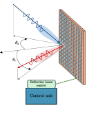
(a)

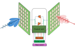
(b)

Figure 1: Illustrative scheme of different SRE components

The relay devices considered in this work include the RIS and the NCR.

The RIS is constructed as a planar metasurface comprising $M$ sub-wavelength meta-atoms, each controlled by a PIN diode or varactor for phase manipulation, as shown in Figure 1a. This configuration enables dynamic reconfiguration and directional reflection, enhancing coverage in obstructed areas. The cost model for an RIS is structured with both a fixed deployment cost and a variable cost that scales linearly with the number of meta-atoms. This linear scaling reflects the increased number of control components (diodes or varactors) and additional circuitry needed as RIS size grows [1], making the cost proportional to the number of meta-atoms. We model the total cost of an RIS as:

$$O^{\mathrm{RIS}}=O^{\mathrm{RIS}}_{d}+O^{\mathrm{RIS}}_{c}\cdot M,$$ (1)

where $O^{\mathrm{RIS}}_{d}$ is the initial deployment cost, and $O^{\mathrm{RIS}}_{c}$ represents the unit cost per meta-atom.

The NCR configuration, depicted in Figure 1b, consists of two antenna panels, each with $N_{p}$ elements. The first panel is oriented toward the BS, while the second panel, facing the target coverage area, is positioned at an angular separation $\alpha$ to prevent loop-back interference, which is essential for effective signal relaying through beamforming and amplification. Operating in TDD mode, NCR s extend signal reach and manage interference, with continuous power consumption that adds to the overall operating cost. Unlike the passive RIS, NCR s require ongoing power for signal amplification and active beamforming, which increases the operational expenditure (OPEX) beyond the initial deployment costs (CAPEX) [1]. Given these factors, the total cost of an NCR includes both a deployment cost and a variable power consumption cost, modeled as a function of its amplification gain $g$:

$$O^{\mathrm{NCR}}=O^{\mathrm{NCR}}_{d}+O^{\mathrm{NCR}}_{g}\cdot[g]_{dB},$$ (2)

where $O^{\mathrm{NCR}}_{d}$ denotes the deployment cost, and $O^{\mathrm{NCR}}_{g}$ represents the cost per dB of gain. The cost models, will be used in this paper for networks planning optimization, as in [12].

To clarify, the cost models used here are rational estimates based on each device’s component and operational needs. Prices are represented in relative units, with a 100 × 100 RIS taken as the baseline at 1 unit. Other device prices are scaled accordingly, emphasizing that relative rather than absolute costs drive the optimization. While actual costs vary with market conditions and production scales, our framework can seamlessly adapt to precise vendor data as it becomes available. Any adjustments in the cost model may affect specific results but do not alter the optimization approach itself, which is independent of exact pricing assumptions.

Antenna arrays are arranged with half-wavelength spacing at the carrier frequency $f_{0}=c/\lambda$, where $c$ is the speed of light, and $\lambda$ is the wavelength. The meta-atoms on the RIS are spaced at intervals of $\lambda/4$.

II-A Signal Model

Let $s\in\mathbb{C}$ be the complex symbol to be transmitted, where $\mathbb{E}[s^{*}s]=\sigma_{s}^{2}$, representing the transmitted power. The transmitted signal is then expressed as

$$\mathbf{x}=\mathbf{f}\,s,$$ (3)

where $\mathbf{f}$ denotes the precoding vector, such that $\|\mathbf{f}\|_{\mathrm{F}}^{2}=N_{t}$. The transmitted signal in (3) is received by the UE directly $\mathbf{r}^{\mathrm{d}}$, through an NCR $\mathbf{r}^{\mathrm{NCR}}$, or via a RIS $\mathbf{r}^{\mathrm{RIS}}$. This is represented as:

$$y=\mathbf{w}^{\mathrm{H}}\left(\mathbf{r}^{\mathrm{d}}+\sum_{i\in\mathcal{I}}\mathbf{r}_{i}^{\mathrm{RIS}}+\sum_{j\in\mathcal{J}}\mathbf{r}_{j}^{\mathrm{NCR}}\right)+\mathbf{w}^{\mathrm{H}}\,\mathbf{n},$$ (4)

where $\mathbf{n}\sim\mathcal{CN}\left(\mathbf{0},\sigma_{n}^{2}\,\mathbf{I}_{N_{r}}\right)$ represents additive white Gaussian noise, $\mathbf{w}\in\mathbb{C}^{N_{r}\times 1}$ is the combining vector, and $\mathcal{I},\mathcal{J}$ denote the sets of deployed RIS s and NCR s, respectively.

II-A1 Direct Signal Model

The received signal for the direct link is:

$$\mathbf{r}^{\mathrm{d}}=\mathbf{H}^{\mathrm{d}}\,\mathbf{x}$$ (5)

with $\mathbf{H}^{\mathrm{d}}\in\mathbb{C}^{N_{r}\times N_{t}}$ representing the MIMO direct channel.

II-A2 Relayed Signal Model via RIS

The received signal for the relayed link through an RIS is expressed as:

$$\mathbf{r}^{\mathrm{RIS}}=\mathbf{H}_{o}^{\mathrm{RIS}}\,\boldsymbol{\Phi}\,\mathbf{H}_{i}^{\mathrm{RIS}}\,\mathbf{x},$$ (6)

with $\boldsymbol{\Phi}\in\mathbb{C}^{M\times M}$ as the reflection coefficient matrix. Here, $\mathbf{H}_{i}^{\mathrm{RIS}}\in\mathbb{C}^{M\times N_{t}}$ and $\mathbf{H}_{o}^{\mathrm{RIS}}\in\mathbb{C}^{N_{r}\times M}$ are the input/output channel matrices between the BS, the RIS, and the UE. The reflection matrix $\boldsymbol{\Phi}$ in (6) is diagonal with entries defined as:

$$\boldsymbol{\Phi}=\text{diag}\left(e^{j\phi_{1}},...,e^{j\phi_{m}},...,e^{j\phi_{M}}\right),$$ (7)

where $\phi_{m}$ is the phase shift applied at the $m$-th element.

II-A3 Relayed Signal Model via NCR

Since the NCR is an active device, the received signal model includes amplified noise. The signal received by the NCR is:

$$\mathbf{z}^{\mathrm{NCR}}=\mathbf{H}_{i}^{\mathrm{NCR}}\,\mathbf{x}+\mathbf{v},$$ (8)

where $\mathbf{v}\in\mathbb{C}^{N_{p}\times 1}\sim\mathcal{CN}\left(\mathbf{0},\sigma_{v}^{2}\,\mathbf{I}_{N_{p}}\right)$ represents the noise at the NCR, and $\mathbf{H}_{i}^{\mathrm{NCR}}\in\mathbb{C}^{N_{p}\times N_{t}}$ is the channel matrix between the BS and the NCR. The signal $\mathbf{z}^{\mathrm{NCR}}$ in (8) is amplified and forwarded towards the UE. The signal received by the UE via the NCR can be expressed as:

$$\mathbf{r}^{\mathrm{NCR}}=\sqrt{g}\,\mathbf{H}_{o}^{\mathrm{NCR}}\,\mathbf{Q}\,\mathbf{z}^{\mathrm{NCR}},$$ (9)

where $g$ denotes the amplification gain, $\mathbf{H}_{o}^{\mathrm{NCR}}\in\mathbb{C}^{N_{r}\times N_{p}}$ is the channel matrix between the NCR and the UE. The relaying matrix $\mathbf{Q}\in\mathbb{C}^{N_{p}\times N_{p}}$ applies a phase shift between the received and forwarded signals. For the NCR configuration, the relaying matrix is:

$$\mathbf{Q}=\mathbf{u}\,\mathbf{b}^{\mathrm{H}},$$ (10)

where $\mathbf{u}\in\mathbb{C}^{N_{p}\times 1}$ and $\mathbf{b}\in\mathbb{C}^{N_{p}\times 1}$ represent the forwarding and receiving beamformers, respectively.

II-B Channel Model

We assume a block-fading channel model with independent fading among direct $\mathbf{H}^{\mathrm{d}}$, forward $\mathbf{H}_{i}$, and backward $\mathbf{H}_{o}$ channels for NCR and RIS. Given the challenging propagation conditions at mmWave frequencies, we adopt the Saleh-Valenzuela cluster-based model (see [16]). The impulse response of any channel in the model can be expressed as:

$$\mathbf{H}=\sum_{p=1}^{P}\frac{\alpha_{p}}{\sqrt{P}}\,\varrho_{r}(\vartheta_{p}^{r},\varphi_{p}^{r})\varrho_{t}(\vartheta_{p}^{t},\varphi_{p}^{t})\mathbf{a}_{r}(\vartheta_{p}^{r},\varphi_{p}^{r})\mathbf{a}_{t}(\vartheta_{p}^{t},\varphi_{p}^{t})^{\mathrm{H}},$$ (11)

where $P$ is the number of paths, $\alpha_{p}$ denotes the scattering amplitude of the $p$-th path, and $\mathbf{a}_{t}(\vartheta_{p}^{t},\varphi_{p}^{t})\in\mathbb{C}^{N_{t}\times 1}$ and $\mathbf{a}_{r}(\vartheta_{p}^{r},\varphi_{p}^{r})\in\mathbb{C}^{N_{r}\times 1}$ denote the Tx and Rx array response vectors for the $p$-th path, which depend on the Tx and Rx pointing angles $(\vartheta_{p}^{t},\varphi_{p}^{t})$ and $(\vartheta_{p}^{r},\varphi_{p}^{r})$. Element radiation patterns $\varrho(\vartheta_{p},\varphi_{p})$ are incorporated according to [17] for BS, UE, and NCR, and are defined as in [18] for the RIS.

Assuming a uniform planar array, the array factor $\mathbf{a}(\vartheta,\varphi)$ in (11) can be expressed as:

$$\mathbf{a}(\vartheta,\varphi)=[e^{j\mathbf{k}(\vartheta,\varphi)^{\mathrm{T}}\boldsymbol{\nu}_{1}},\cdots,e^{j\mathbf{k}(\vartheta,\varphi)^{\mathrm{T}}\boldsymbol{\nu}_{L}}],$$ (12)

where $\mathbf{k}(\vartheta,\varphi)\in\mathbb{R}^{3\times 1}$ is the wave vector, defined as:

$$\mathbf{k}(\vartheta,\varphi)=\frac{2\pi}{\lambda}[\cos(\varphi)\cos(\vartheta),\cos(\varphi)\sin(\vartheta),\sin(\varphi)]^{T},$$ (13)

and $\boldsymbol{\nu}_{\ell}=[x_{\ell},y_{\ell},z_{\ell}]$ represents the position of the $\ell$-th element in the array, in local coordinates.

Using the calculated direct or relay channels, we can compute the instantaneous signal-to-noise ratio (SNR) for each link, denoted by $\gamma_{0}$, following the approach in [11]. Static blockage is handled deterministically using actual building maps to form the scenario, while the dynamic blockage model from [15] is used for long-term SNR calculations. For example, for the direct path, the long-term SNR is calculated as in [11]:

$$\overline{\gamma}^{\textrm{BS}}=\mathrm{P}^{\textrm{BS}}_{B}\,\gamma^{\textrm{BS}}+(1-\mathrm{P}^{\textrm{BS}}_{B})\gamma_{0}^{\textrm{BS}},$$ (14)

where $\mathrm{P}^{\textrm{BS}}_{B}$ is the blockage probability of the direct paths, $\gamma_{0}^{\textrm{BS}}$ is the SNR upper limit when blockage does not occur, and ${\gamma}^{\textrm{BS}}$ is the SNR accounting for penetration loss or knife-edge diffraction [11, 19]. The long-term SNR for relayed links is calculated similarly. The dynamic blockage probability $\mathrm{P}_{B}$ depends on link length, as well as parameters like blocker density, velocity, and dimensions [15]. These long-term SNR s are used by the optimization models presented in the next section.

III Cost Minimization

The mmW SRE-based networks depend significantly on deployment geometry, which directly impacts performance, as shown in previous planning studies [14]. Due to the potential for large-scale deployments resulting from the cost-efficiency of these devices, understanding system-level impacts is essential. To precisely assess network performance with these devices integrated, we employ a Mixed Integer-Linear Programming (MILP) optimization approach. This approach ensures an optimal deployment layout, providing performance insights that reflect the best possible outcomes for networks using RIS and NCR devices. The objective is to minimize network costs while ensuring full coverage.

III-A System Model

Consider a geographic area where the coverage of a pre-deployed BS requires enhancement through SRE devices. Let $\mathcal{C}$ represent the set of Candidate Sites (CSs) for potential SRE device installations.

This work considers two types of SRE devices, RIS and NCR, with distinct performance metrics and costs. The MILP approach optimizes network planning by choosing between these device types at each CS to maximize planning objectives. This is mathematically modeled with the set $\mathcal{D}$, which represents available technologies (RIS or NCR) and configurations, such as RIS size or NCR amplification gain.

Let $\mathcal{T}$ denote the set of TPs, representing sampled positions in the geographic area where coverage is evaluated. Each TP $t\in\mathcal{T}$ is considered covered if the SNR at that location exceeds a threshold $\Gamma$. This threshold, representing the minimum guaranteed SNR enforced at each TP, is determined prior to planning optimization and shapes the final network topology.

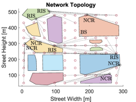
(a)

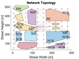
(b)

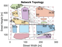
(c)

Figure 2: Optimally planned network topologies for minimizing total installation cost, for the scenario of Piazza Piola in Milan I, varying the the guaranteed number of connections for each test point $K$ and SNR threshold in dB $\Gamma$, using the default parameters in Table I.

The measured SNR depends on the final network topology and active SRE devices. Each TP $t\in\mathcal{T}$ can be served either directly by the BS or indirectly through an SRE device. Let $\overline{\gamma}^{\text{BS}}_{t}$ represent the long-term SNR measured at TP $t$ from the BS only. Using the channel model from Sect. II-B, we define a boolean activation parameter $\Delta_{t}^{\text{BS}}$ as follows:

$$\Delta_{t}^{\text{BS}}=\left\{\begin{array}[]{@{}ll@{}}1,&\text{if}\ \overline{\gamma}_{t}^{\text{BS}}\geq\Gamma\\ 0,&\text{otherwise.}\end{array}\right.$$ (15)

This indicates that $\Delta_{t}^{\text{BS}}$ is 1 if the BS can meet the SNR threshold at TP $t$, and 0 otherwise.

Similarly, we calculate the SNR at each TP from active SRE devices, defining $\overline{\gamma}_{t,c}^{d}$ as the SNR at TP $t$ from a device of type $d\in\mathcal{D}$ at CS $c\in\mathcal{C}$. The activation parameter $\Delta_{t,c}^{d}$ is defined as:

$$\Delta_{t,c}^{d}=\left\{\begin{array}[]{@{}ll@{}}1,&\text{if}\ \overline{\gamma}_{t,c}^{d}\geq\Gamma\\ 0,&\text{otherwise}\end{array}\right.$$ (16)

These activation parameters ($\Delta_{t}^{\text{BS}}$ and $\Delta_{t,c}^{d}$) inform the optimization model about feasible coverage links. They can also be adjusted to account for obstructions or other deployment constraints.

III-B Optimization Formulation

During the optimization phase, we define $O^{d}$ as the cost of installing a device of type $d\in\mathcal{D}$. We then define the decision variable $v_{c}^{d}\in\{0,1\}$, where $v_{c}^{d}=1$ if a device of type $d$ is installed at CS $c$, and $v_{c}^{d}=0$ otherwise. The optimization formulation is as follows:

$$\min\sum_{c\in\mathcal{C},d\in\mathcal{D}}O^{d}v_{c}^{d}$$ (17a)

s.t. $$\Delta_{t}^{\text{BS}}+\sum_{c\in\mathcal{C},d\in\mathcal{D}}\Delta_{t,c}^{d}v_{c}^{d}\geq K\quad\forall t\in\mathcal{T}$$ (17b)

$$v_{c}^{d}\in\{0,1\}\quad\forall c\in\mathcal{C},d\in\mathcal{D}$$ (17c)

In (17a), the objective function minimizes network costs by optimizing device installations. Constraint (17b) ensures each TP is covered by at least $K$ distinct devices, achieving the required SNR. Although computationally intensive, this formulation effectively addresses realistic planning scenarios, as discussed in Sect. IV.

IV Results

TABLE I: Default simulation parameters used in Section IV.

Parameter	Symbol	Value(s)
Carrier frequency	$f_{0}$	$28$ GHz
Bandwidth	$B$	$200$ MHz
BS Transmit power	$\sigma^{2}_{s}$	$35$ dBm
Noise power	$\sigma^{2}_{n}$	$-82$ dBm
NCR array size	$N_{p,h}\times N_{p,v}$	$12\times 6$
NCR amplification gain	$|g|^{2}$	$55$ dB
RIS elements	$\sqrt{M}\times\sqrt{M}$	$100\times 100$
RIS element spacing	$d_{n},d_{m}$	$\lambda_{0}/4$ m
BS antenna array	$N_{\mathrm{t}}$	$12\times 16$
Device prices	$O^{\mathrm{ris}}$, $O^{\mathrm{ncr}}$	1, 3
Blocker height [15]	$h_{B}$	1.7 m
Blocker density [15]	$\lambda_{B}$	$4\times 10^{-3}$ m-2
Blocker velocity [15]	$V$	15 m/s
Blockage duration [15]	$\mu^{-1}$	5 s

In this section we provide numerical results, achieved with the optimization model (17). For simplicity, we assume a uniform building height of 6 meters due to limited data on specific heights. Building shapes are convexified as in [20], preserving spatial accuracy while streamlining the network planning process. RIS CSs are positioned at a height of 5 meters on building walls, while NCR CSs are set at 6.5 meters, reflecting the rooftop placement. The candidate sites (CSs) for RIS s are spaced at regular intervals of 5 meters along building walls. For NCR s, CSs are chosen from rooftop vertices, with one panel facing the BS and the other directed toward target coverage areas. The default simulation parameters are provided in Table I, unless specified otherwise.

We begin by presenting the optimally planned network topologies for an exemplary scenario at Piazza Piola in Milan, illustrated in Figure 2. To examine the impact of varying network requirements, we adjust the guaranteed number of connections for each TP, denoted as $K$, and the SNR threshold, $\Gamma$, measured in dB. The specific values of these parameters are detailed in the figure captions.

In the scenario with $K=1$ and $\Gamma=0$ dB in Figure (a), a total of 4 RIS s and 5 NCR s are deployed, resulting in a total cost of 19 units. Increasing the SNR threshold to 20 dB in Figure (b) prompts the optimization model to deploy 5 RIS s and 10 NCR s, raising the total cost to 35 units. Alternatively, increasing the number of paths each TP can be served by to $K=2$ (Figure (c)) results in the deployment of 7 RIS s and 10 NCR s, with a total cost of 37 units.

In each scenario, not only the number of devices changes, but also most of the times, the model chooses different CS s to install them. These results indicate that as the SNR threshold increases, the model tends to prioritize NCR installations due to their amplification gain, which better supports higher SNR demands.

In the next step, to obtain broader, non-site-specific results, we apply the optimization model across eight distinct $400\times 400$ m regions within the Milan map. In each region, a single BS is positioned near the center on top of a building.

To begin, we fix the default configurations for both devices and examine how the total cost of achieving 100% coverage of the TPs s scales with the price ratio of NCR to RIS, represented as $\ O^{\mathrm{NCR}}/\ O^{\mathrm{RIS}}$. Figure 3 illustrates the total cost versus the NCR-to-RIS price ratio, with device configurations set to the default values in Table I. The gray dashed lines in the figures denote each region, while shaded areas represent the upper and lower bounds derived from these regions. The thick solid lines with markers indicate the average values across scenarios.

As the price ratio increases, the total cost for each region, along with the average total cost, shows an exponential trend. This trend is particularly pronounced due to the requirement that all TPs be served. For TPs located at a distance from the BS or obstructed by buildings, service can only be provided by NCR devices, which, despite their higher cost, are essential for extending coverage in such challenging areas. Specifically, with SNR threshold $\Gamma=0$ dB, if the cost ratio exceeds $\ O^{ncr}/\ O^{ris}>1.3$, the contribution of RIS s surpasses that of NCR s. For SNR threshold $\Gamma=10$ dB, even when the ratio exceeds $\ O^{ncr}/\ O^{ris}>3$, the contribution of NCR s remains higher than that of RIS s, due to the high SNR requirements that only NCR s can satisfy, regardless of price.

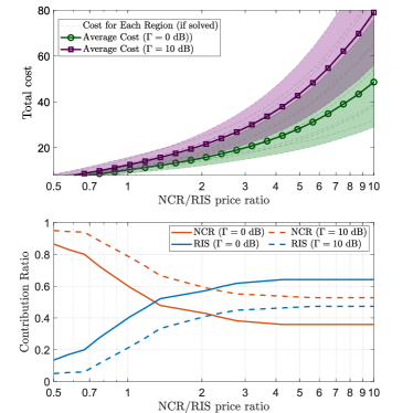
Figure 3: Average total cost vs NCR/RIS price ratio with FCMC optimization model, for fixed settings of RIS/NCR (see Table I).

Having fixed the default configurations of the devices in the previous example, in the next examples, we scale the price of RIS, according to the relation (1) with the initial deployment cost $O^{\mathrm{RIS}}_{d}=0.4$, and cost per meta-atom $O^{\mathrm{RIS}}_{c}=6\times 10{-5}$, and we scale the price of NCR according to relation (2) with the deployment cost $O^{\mathrm{NCR}}_{d}=0.8$ , and cost per dB of gain $O^{\mathrm{NCR}}_{g}=4\times 10^{-2}$. As mentioned in Section II, these values are assumed such that a RIS with a default dimension of $M=100\times 100$ costs 1 unit, while a NCR with default parameters would cost more expensive. The rational behind such models lies in their used components [1].

We first vary the RIS configuration, keeping the NCR gain fixed. Figure 4 shows the total cost versus RIS dimension, $\sqrt{M}$. For RIS configurations ranging from $M=50\times 50$ to $M=150\times 150$, full coverage is achievable with reduced cost, although increasing dimensions beyond certain points begins to raise costs. Optimized configurations show approximately 20% cost reduction in certain cases.

Similarly, we examine how NCR gain impacts total cost, keeping RIS configuration fixed. Figure 5 shows that the minimum cost occurs around $g=38$ dB for $\Gamma=0$ dB, and $g=48$ dB for $\Gamma=10$ dB. Gains above optimal levels only increase total costs without improving coverage. This trend demonstrates that efficient cost management can be achieved by balancing RIS configurations and NCR gain.

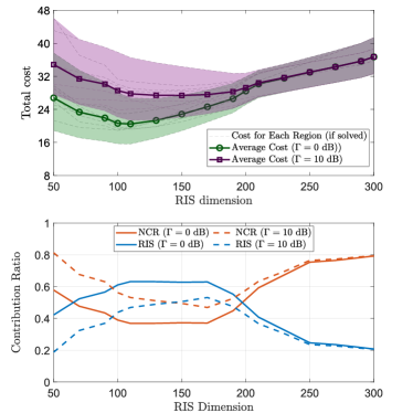
Figure 4: Average total cost vs RIS dimension where the configurations and price of the NCR is the default according to Table I and the cost of the RIS scales according to relation (1).

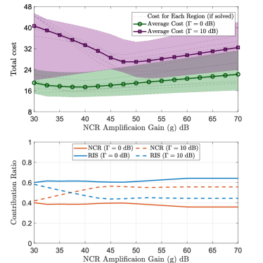
Figure 5: Average total cost vs NCR gain, where the configuration and price of the RIS is the default according to Table I and the cost of the NCR scales according to relation (2).

V Conclusion

This paper presented an optimized deployment framework for HSRE networks, designed to minimize infrastructure costs while ensuring full coverage in urban environments. By integrating RIS and NCR devices and considering realistic environmental constraints, our approach effectively meets the high connectivity demands of dense urban areas. Through the proposed cost-minimization model, we demonstrated that balancing device configurations—such as RIS dimensions and NCR amplification gain—significantly impacts overall deployment costs, particularly under varying SNR thresholds and connectivity requirements. In future work, we aim to explore an alternative optimization method to maximize coverage within a fixed budget, and to expand our framework to incorporate additional SRE devices beyond RIS and NCR, further enhancing network planning flexibility.

References

- [1] R. Flamini, D. De Donno, J. Gambini, F. Giuppi, C. Mazzucco, A. Milani, and L. Resteghini, “Towards a heterogeneous smart electromagnetic environment for millimeter-wave communications: An industrial viewpoint,” IEEE Transactions on Antennas and Propagation, pp. 1–1, 2022.
- [2] N. yu, P. Genevet, M. Kats, F. Aieta, J.-P. Tetienne, F. Capasso, and Z. Gaburro, “Light propagation with phase discontinuities: Generalized laws of reflection and refraction,” Science (New York, N.Y.), vol. 334, pp. 333–7, 09 2011.
- [3] F. I. G. Carvalho, R. V. de O. Paiva, T. F. Maciel, V. F. Monteiro, F. R. M. Lima, D. C. Moreira, D. A. Sousa, B. Makki, M. Astrom, and L. Bao, “Network-controlled repeater – an introduction,” 2024.
- [4] G. C. M. Da Silva, D. A. Sousa, V. F. Monteiro, D. C. Moreira, T. F. Maciel, F. R. M. Lima, and B. Makki, “Impact of network deployment on the performance of ncr-assisted networks,” in 2024 19th International Symposium on Wireless Communication Systems (ISWCS), 2024, pp. 1–6.
- [5] Y. Ren, R. Zhou, X. Teng, S. Meng, M. Zhou, W. Tang, X. Li, C. Li, and S. Jin, “On deployment position of ris in wireless communication systems: Analysis and experimental results,” IEEE Wireless Communications Letters, vol. 12, no. 10, pp. 1756–1760, 2023.
- [6] K. Ntontin, D. Selimis, A.-A. A. Boulogeorgos, A. Alexandridis, A. Tsolis, V. Vlachodimitropoulos, and F. Lazarakis, “Optimal reconfigurable intelligent surface placement in millimeter-wave communications,” in 2021 15th European Conference on Antennas and Propagation (EuCAP), 2021, pp. 1–5.
- [7] S. Bagherinejad, M. Bayanifar, M. Sattari Maleki, and B. Maham, “Coverage probability of ris-assisted mmwave cellular networks under blockages: A stochastic geometric approach,” Physical Communication, vol. 53, p. 101740, 2022. [Online]. Available: https://www.sciencedirect.com/science/article/pii/S1874490722000805
- [8] A. H. A. Bafghi, M. Mirmohseni, M. Nasiri-Kenari, B. Maham, and U. Spagnolini, “Stochastic analysis of homogeneous wireless networks assisted by intelligent reflecting surfaces,” 2024.
- [9] J. Zhang and D. M. Blough, “Optimizing coverage with intelligent surfaces for indoor mmwave networks,” in IEEE INFOCOM 2022 - IEEE Conference on Computer Communications. IEEE Press, 2022, p. 830–839.
- [10] G. C. M. da Silva, E. R. B. Falcão, V. F. Monteiro, D. C. Moreira, D. A. Sousa, T. F. Maciel, F. R. M. Lima, and B. Makki, “System level evaluation of network-controlled repeaters: Performance improvement of serving cell and interference impact on neighbor cells,” 2023.
- [11] R. A. Ayoubi, M. Mizmizi, D. Tagliaferri, D. D. Donno, and U. Spagnolini, “Network-controlled repeaters vs. reconfigurable intelligent surfaces for 6g mmw coverage extension: A simulative comparison,” in 2023 21st Mediterranean Communication and Computer Networking Conference (MedComNet), 2023, pp. 196–202.
- [12] E. Moro, I. Filippini, A. Capone, and D. De Donno, “Planning mm-wave access networks with reconfigurable intelligent surfaces,” in 2021 IEEE 32nd Annual International Symposium on Personal, Indoor and Mobile Radio Communications (PIMRC), 2021, pp. 1401–1407.
- [13] P. Fiore, E. Moro, I. Filippini, A. Capone, and D. D. Donno, “Boosting 5g mm-wave iab reliability with reconfigurable intelligent surfaces,” in 2022 IEEE Wireless Communications and Networking Conference (WCNC), 2022, pp. 758–763.
- [14] G. Leone, E. Moro, I. Filippini, A. Capone, and D. D. Donno, “Towards Reliable mmWave 6G RAN: Reconfigurable Surfaces, Smart Repeaters, or Both?” in International Symposium on Modeling and Optimization in Mobile, Ad hoc, and Wireless Networks, WiOpt , Turin, Italy, 2022.
- [15] I. K. Jain, R. Kumar, and S. S. Panwar, “The impact of mobile blockers on millimeter wave cellular systems,” IEEE Journal on Selected Areas in Communications, vol. 37, no. 4, pp. 854–868, 2019.
- [16] A. F. Molisch, Channel Models, 2011, pp. 125–143.
- [17] 3GPP ETSI TR 138 900, “Study on channel model for frequency spectrum above 6 GHz (version 14.2.0 Release 14),” Jun 2017.
- [18] M. Mizmizi, R. A. Ayoubi, D. Tagliaferri, K. Dong, G. G. Gentili, and U. Spagnolini, “Conformal metasurfaces: a novel solution for vehicular communications,” IEEE Transactions on Wireless Communications, 2022.
- [19] 3GPP, “Study on channel model for frequencies from 0.5 to 100 ghz (release 16),” 2019.
- [20] R. Aghazadeh Ayoubi, D. Tagliaferri, F. Morandi, L. Rinaldi, L. Resteghini, C. Mazzucco, and U. Spagnolini, “Imt to satellite stochastic interference modeling and coexistence analysis of upper 6 ghz-band service,” IEEE Open Journal of the Communications Society, vol. 4, pp. 1156–1169, 2023.