GaussianSpa: An “Optimizing-Sparsifying” Simplification Framework for Compact and High-Quality 3D Gaussian Splatting

Abstract

3D Gaussian Splatting (3DGS) has emerged as a mainstream for novel view synthesis, leveraging continuous aggregations of Gaussian functions to model scene geometry. However, 3DGS suffers from substantial memory requirements to store the multitude of Gaussians, hindering its practicality. To address this challenge, we introduce GaussianSpa, an optimization-based simplification framework for compact and high-quality 3DGS. Specifically, we formulate the simplification as an optimization problem associated with the 3DGS training. Correspondingly, we propose an efficient “optimizing-sparsifying” solution that alternately solves two independent sub-problems, gradually imposing strong sparsity onto the Gaussians in the training process. Our comprehensive evaluations on various datasets show the superiority of GaussianSpa over existing state-of-the-art approaches. Notably, GaussianSpa achieves an average PSNR improvement of 0.9 dB on the real-world Deep Blending dataset with 10$\times$ fewer Gaussians compared to the vanilla 3DGS. Our project page is available at https://gaussianspa.github.io/.

1 Introduction

Novel view synthesis has become a pivotal area in computer vision and graphics, driving advancements in applications such as virtual reality, augmented reality, and immersive media experiences [21]. NeRF [35] has recently gained prominence in this domain because it can generate high-quality, photorealistic images from sparse input views by representing scenes as continuous volumetric functions based on neural networks. However, NeRF often requires extensive computational resources and long training times, making it less practical for real-time applications and large-scale reconstructions.

3D Gaussian Splatting (3DGS) [25] has emerged as a powerful alternative, leveraging continuous aggregations of Gaussian functions to model scene geometry and appearance. Unlike NeRF, which relies on neural networks to approximate volumetric radiance fields, 3DGS directly represents scenes using a collection of Gaussians. This approach excels in capturing details and smooth transitions, offering significant advantages in training and rendering speed. 3DGS achieves superior visual fidelity [28] compared to NeRF while reducing computational overhead, making it more suitable for interactive applications that demand quality and performance.

Despite its strengths, 3DGS suffers from significant memory requirements that hinder its practicality. The main issue is the massive memory consumption associated with storing a large number of Gaussians that are needed to represent complex scenes. Each Gaussian occupies memory space for its parameters, including position, covariance, and color attributes. In densely sampled scenes, the sheer volume of Gaussians leads to memory usage that exceeds the capacity of typical hardware, making it challenging to handle higher-resolution scenes and limiting its applicability in resource-constrained environments.

Existing works, e.g., Mini-Splatting [20], LightGaussian [19], LP-3DGS [54], EfficientGS [31], and RadSplat [40], have predominantly focused on mitigating this issue by removing a certain number of Gaussians. Techniques such as pruning and sampling aim to discard unimportant Gaussians based on hand-crafted criteria such as opacity [25, 53], importance score (hit count) [20, 19, 40], dominant primitives [31], and binary mask [54, 29]. However, these criteria are generally utilized to determine the importance of Gaussian points from a single heuristic perspective, limiting robustness in dynamic scenes or under varying lighting conditions. Moreover, the sudden one-shot removal may cause permanent loss of Gaussians that are crucial to visual synthesis, making it challenging to recover the original performance after even long-term training, as shown in Figure 2. Consequently, while these methods can alleviate memory and storage burdens to some extent, they often lead to sub-optimal rendering outcomes with loss of details and visual artifacts, thereby compromising the quality of the synthesized views.

In this paper, we present an optimization-based simplification framework, GaussianSpa, for compact and high-quality Gaussian Splatting. In the proposed framework, we formulate 3DGS simplification as a constrained optimization problem under a target number of Gaussians. Then, we propose an efficient “optimizing-sparsifying” solution for the formulated problem by splitting it into two simple sub-problems that are alternately solved in the “optimizing” step and the “sparsifying” step. Instead of permanently removing a certain number of Gaussians, GaussianSpa incorporates the “optimizing-sparsifying” algorithm into the training process, gradually imposing a substantial sparse property onto the trained Gaussians. Hence, our GaussianSpa can simultaneously enjoy maximum information preservation from the original Gaussians and a desired number of reduced Gaussians, providing compact 3DGS models with high-quality rendering. Overall, our contributions can be summarized as follows:

• We propose a general 3DGS simplification framework that formulates the simplification objective as an optimization problem and solves it in the 3DGS training process. In solving the formulated optimization problem, our proposed framework gradually restricts Gaussians to the target sparsity constraint without explicitly removing a specific number of points. Hence, GaussianSpa can maximally maintain and smoothly transfer the information to the sparse Gaussians from the original model.

• We propose an efficient “optimizing-sparsifying” solution for the formulated problem, which can be integrated into the 3DGS training with negligible costs, separately solving two sub-problems. In the “optimizing” step, we optimize the original loss function attached by a regularization with gradient descent. In the “sparsifying” step, we analytically project the auxiliary Gaussians onto the constrained sparse space.

• We comprehensively evaluate GaussianSpa through extensive experiments on various complex scenes, demonstrating improved rendering quality compared to existing approaches. Particularly, with as high as 10$\times$ fewer number of Gaussians than the vanilla 3DGS, GaussianSpa achieves an average 0.4 dB improvement on the Mip-NeRF 360 [4] and Tanks&Temples [27] datasets, 0.9 dB on Deep Blending [23] dataset. Furthermore, we conduct various visual quality assessments, showing that GaussianSpa exhibits high-quality rendering of details and sparse 3D Gaussian views.

2 Related Work

2.1 Novel View Synthesis

Novel View Synthesis (NVS) [2] is a technique in computer vision and graphics to generate images of a 3D scene from unseen viewpoints based on existing multi-view data. A seminal work in this field is NeRF [35], which uses an implicit neural network to represent a scene as a continuous 5-dimensional function, mapping 3D coordinates and viewing directions to color and density. NeRF introduces positional encoding and a hierarchical sampling strategy to improve the ability of the MLP [6] to represent high-frequency image details and accelerate the rendering process. However, NeRF’s reliance on single narrow-ray sampling poses challenges in addressing aliasing and blur artifacts. To mitigate this, Mip-NeRF [3] represents the scene at a continuous-valued scale, enabling anti-aliased rendering by casting conical frustums from each pixel at various scales. Additionally, Mip360 [4] extends NeRF’s capabilities to unbounded scenes, utilizing a non-linear scene parameterization, online distillation, and a novel distortion-based regularizer. More recently, an explicit point-based method, 3D Gaussian Splatting (3DGS), which leverages continuous aggregations of Gaussian functions to model scene geometry, has emerged as a point-based alternative, demonstrating significant improvements in rendering quality and speed.

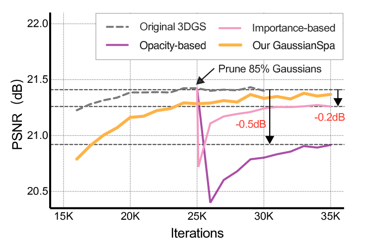
Figure 2: PSNR curves of human-crafted criteria-based pruning methods. All methods remove 85% of the Gaussians at iteration 25K.

2.2 Efficient 3DGS

3DGS significantly improves rendering quality and computational efficiency compared to traditional methods such as NeRF [35], which are often resource-intensive and computationally slow. However, the demands of real-time rendering and the reconstruction of unbounded, large-scale 3D scenes underscore the requirement for model efficiency [10]. Optimization for 3DGS focuses on four main categories to effectively reduce model size: Gaussian simplification, vector quantization, spherical harmonics optimization, and hybrid compression.

Gaussian Simplification. Gaussian simplification involves removing Gaussians to compress 3DGS models into compact forms, significantly reducing memory costs. Prior approaches [20, 40, 34, 54, 32, 46, 30, 13, 26] mainly focus on pruning redundant Gaussians according to hand-crafted importance criteria. Mini-Splatting [20] introduces blur splitting and depth reinitialization to address overlapping and under-reconstructed problems, using stochastic sampling to better preserve geometry based on importance scores. Radsplatting [40] computes an importance score by aggregating ray contributions of Gaussians across all input images, replacing summation with a max operator for robustness to varying scene coverage. Taming 3DGS [34] implements steerable densification by calculating scores based on pixel saliency, gradients, and Gaussian attributes, then selectively cloning or splitting high-scoring Gaussians. LP-3DGS [54] applies a trainable binary mask with Gumbel-Sigmoid to automatically optimize pruning, improving efficiency while maintaining quality.

Vector Quantization. Vector quantization [50] aims to compress data using discrete entries from a learned codebook, reducing data redundancy. Several works [22, 38, 12, 51, 42, 36, 39] apply vector quantization for compressing 3DGS models. For instance, EAGLES [22] quantizes attributes like spherical harmonics (SH) coefficients and opacity to create latent representations for per-point compression, using an MLP decoder to reconstruct the original attributes with high fidelity. CompGS [38] applies a K-means-based vector quantization approach to compress 3DGS parameters, significantly reducing storage and rendering time with minimal quality loss. RDO-Gaussian [51] performs end-to-end rate-distortion optimization for 3D Gaussian Splatting, combining dynamic pruning and entropy-constrained vector quantization to reduce storage while maintaining quality.

Spherical Harmonics Optimization. Among 3DGS parameters, spherical harmonics (SH) coefficients take up a significant portion, requiring (45+3) floating-point values per Gaussian for a degree of 3 (as used in [25]), which accounts for around 80% of the total attribute volume. Prior works [19, 29] optimize SH coefficients to reduce storage overhead. For instance, EfficientGS [31] retains zeroth-order SH for all Gaussians, increasing the order when necessary.

Hybrid Compression. In addition to methods focused on individual aspects of 3DGS compression, several recent approaches [19, 31, 29, 52] combine multiple techniques for hybrid compression to achieve further storage reduction. LightGaussian [19] prunes 3DGS points using a global importance score, applies vector quantization to compress SH coefficients, and reduces SH degree through knowledge distillation combined with pseudo-view augmentation. EfficientGS [31] not only keeps zeroth-order SH for all Gaussians, increasing the order only when needed but also classifies Gaussians into steady and non-steady states, densifying non-steady Gaussians while retaining only the top-K most important Gaussians per ray. CompactGaussian [29] introduces a learnable mask to mark redundant Gaussians and residual vector quantization for scale and rotation and replaces SH with a grid-based neural field to represent colors.

Although these methods improve 3DGS efficiency, they lead to irreversible information loss during the Gaussian simplification process. Specifically, those methods perform simplification by a one-shot pruning on the Gaussians without prominent sparse characteristics, causing a notable PSNR degradation that is challenging to recover, as shown in Figure 2. Consequently, when applying additional compressions like SH optimization and vector quantization after simplification, the compressed 3DGS model often exhibits further performance loss due to the accumulated errors. Our work focuses on Gaussian simplification by formulating it as an optimization problem and imposing substantial sparsity onto Gaussians, mitigating performance issues with improved rendering quality at the first stage to achieve efficient 3DGS.

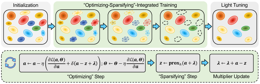
Figure 3: Overall workflow of our proposed GaussianSpa framework.

3 Methodology: GaussianSpa

3.1 Background of 3D Gaussian Splatting

3D Gaussian Splatting (3DGS) explicitly represents scenes using a collection of point-based 3D continuous Gaussians. Specifically, each Gaussian $G$ is characterized by its covariance matrix $\bm{\Sigma}$ and center position $\bm{\mu}$ as

$$G(\bm{x})=\exp\left(-\frac{1}{2}(\bm{x}-\bm{\mu})^{\top}\bm{\Sigma}^{-1}(\bm{x}-\bm{\mu})\right),$$ (1)

where $\bm{x}$ is an arbitrary location in the 3D scene. The covariance matrix $\bm{\Sigma}$ is generally composed of $\bm{\Sigma}=\bm{R}\bm{S}\bm{S}^{\top}\bm{R}^{\top}$ with a rotation matrix $\bm{R}$ and a scale matrix $\bm{S}$, ensuring the positive definite property. Additionally, each Gaussian is associated with an opacity $a$ and spherical harmonics (SH) coefficients.

When rendering a 2D image from the 3D scene at a certain camera angle, 3DGS projects 3D Gaussians to that 2D plane and calculates the projected 2D covariance matrix by

$$\bm{\Sigma^{\prime}}=\bm{J}\bm{W}\bm{\Sigma}\bm{W}^{\top}\bm{J}^{\top},$$ (2)

where $\bm{W}$ is the view transformation, and $\bm{J}$ is the Jacobian of the affine approximation of the projective transformation [55]. Then, for each pixel on the 2D image, the color $C$ is computed by blending all $N$ ordered Gaussians contributing to the pixel as

$$C=\sum_{i\in N}c_{i}\alpha_{i}\prod_{j=1}^{i-1}(1-\alpha_{j}).$$ (3)

Here, $c_{i}$ and $\alpha_{i}$ denote the view-dependent color computed from the corresponding SH coefficients and the rendering opacity calculated by the Gaussian opacity $a_{i}$, respectively, corresponding to the $i$-th Gaussian.

In the training process [25], the Gaussians are initialized from a sparse point cloud generated by Structure-from-Motion (SfM) techniques [47]. Then, the number of Gaussians is adjusted by a densification algorithm [25] according to the reconstruction geometry. Afterward, each Gaussian’s variables, including the center position, rotation matrix, scaling matrix, opacity, and SH coefficients, are optimized by minimizing the reconstruction errors using the standard gradient descent. Specifically, the loss $\mathcal{L}$ is given by

$$\mathcal{L}=(1-\rho)\mathcal{L}_{1}+\rho\mathcal{L}_{\text{D-SSIM}},$$ (4)

where $\mathcal{L}_{1}$ and $\mathcal{L}_{\text{D-SSIM}}$ are the $\ell_{1}$ norm and the structural dissimilarity between the rendered output and the ground truth, respectively. $\rho$ is a parameter that controls the tradeoff between the two losses.

3.2 Problem Formulation: Simplification as Constrained Optimization

To mitigate irreversible information loss caused by existing one-shot criterion-based pruning, our key innovation is to gradually impose substantial sparsity onto the Gaussians and maximally preserve information in the training process. Mathematically, considering a general 3DGS training, we introduce a sparsity constraint on the Gaussians to the training objective, $\min\mathcal{L}$. Thus, the 3DGS training is reformulated as another constrained optimization problem, the primary formulation of our proposed simplification framework, i.e.,

$$\min{} \mathcal{L},$$ (5)

s.t. $$\mathcal{N}(\bm{G})\leq\kappa.$$

The introduced constraint $\mathcal{N}(\cdot)\leq\kappa$ restricts the number of Gaussians no greater than a target number $\kappa$.

However, the above problem cannot be solved because the Gaussians are continuous functions instead of differentiable variables. Recalling the rendering process with Eq. 3, the contribution of the $i$-th Gaussians to a particular pixel is finally determined by its opacity $a_{i}$. Alternatively, the original sparsity constraint directly on the Gaussians can be explicitly transformed into a sparsity constraint on the opacity variables. As each Gaussian only has one opacity variable, we can use a vector $\bm{a}$ to represent all the opacities and easily restrict its number of non-zeros with $\ell_{0}$ norm, $\|\bm{a}\|_{0}$. For better presentation, we use a variable set $\bm{\Theta}$ to represent other GS variables except for the opacity $\bm{a}$. Hence, the constrained optimization problem can be reformulated as

$$\min_{\bm{a},\bm{\Theta}}{} \mathcal{L}(\bm{a},\bm{\Theta}),$$ (6)

s.t. $$\|\bm{a}\|_{0}\leq\kappa.$$

With this reformulation, we have simplified the primary problem to another form that our proposed “optimizing-sparsifying” can efficiently solve.

3.3 “Optimizing-Sparsifying” Solution

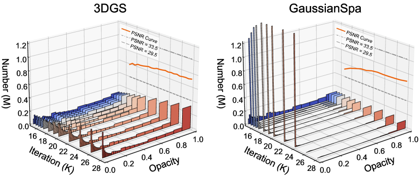
Figure 4: Evolution of opacity distribution and PSNR for 3DGS and GaussianSpa. The “optimizing-sparsifying” starts at iteration 15K. At iteration 25K, GaussianSpa removes “zero” Gaussians, followed by a light tuning.

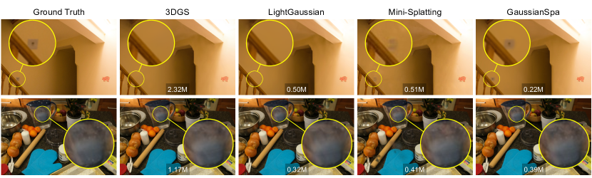
Figure 5: Visual quality results on the Drjohnson and Counter scenes, compared to existing simplification approaches and vanilla 3DGS. The numbers of remaining Gaussians are displayed. It is observed that our GaussianSpa recovers details closest to the ground truth in the actual rendering outcomes with a significantly reduced number of Gaussians.

In this subsection, we present an efficient “optimizing-sparsifying” solution for problem Eq. 6. The key idea is to split it into two simple sub-problems separately solved in an “optimizing” step and a “sparsifying” step alternately.

In order to deal with the non-convex constraint, $\|\bm{a}\|_{0}\leq\kappa$, we first introduce an indicator function,

$$h(\bm{a})=\left\{\begin{matrix}0,&\|\bm{a}\|_{0}\leq\kappa,\\ +\infty,&\textup{otherwise},\\ \end{matrix}\right.$$ (7)

to the minimization objective and remove the sparsity constraint. Thus, problem Eq. 6 becomes an unconstrained optimization form, i.e.,

$$\min_{\bm{a},\bm{\Theta}}~{}\mathcal{L}(\bm{a},\bm{\Theta})+h(\bm{a}).$$ (8)

Here, the first term is the original 3DGS training objective, which is easy to handle, while the second term is still non-differentiable. This makes the above problem unable to solve using gradient descent under existing training frameworks such as PyTorch [44] and TensorFlow [1]. To decouple the two terms, we further introduce an auxiliary variable $\bm{z}$, whose size is identical to $\bm{a}$, and convert Eq. 8 as

$$\min_{\bm{a},\bm{z},\bm{\Theta}}{} \mathcal{L}(\bm{a},\bm{\Theta})+h(\bm{z}),$$ (9)

s.t. $$\bm{a}=\bm{z}.$$

The above problem becomes another constrained problem with an equality constraint. Thus, the corresponding dual augmented Lagrangian [7] form can be given by

$$L(\bm{a},\bm{z},\bm{\Theta},\bm{\lambda};\delta)=\mathcal{L}(\bm{a},\bm{\Theta})+h(\bm{z})+\frac{\delta}{2}\|\bm{a}-\bm{z}+\bm{\lambda}\|^{2}+\frac{\delta}{2}\|\bm{\lambda}\|^{2},$$ (10)

where $\bm{\lambda}$ is the dual Lagrangian multiplier, and $\delta$ is the penalty parameter. Correspondingly, we can separately optimize over the 3DGS variables, $\bm{a},\bm{\Theta}$, and the auxiliary variable, $\bm{z}$, in the augmented Lagrangian, then solve two split sub-problems in an “optimizing” step and a “sparsifying” step alternately.

$$\RHD~{}\textbf{``Optimizing" Step:~{}~{}}\min_{\bm{a},\bm{\Theta}}\mathcal{L}(\bm{a},\bm{\Theta})+\frac{\delta}{2}\|\bm{a}-\bm{z}+\bm{\lambda}\|^{2}.$$ (11)

In the “optimizing” step, the minimization objective, Eq. 11, targets only 3DGS variables and contains two terms, which are the original 3DGS loss function and a quadratic regularization that enforces the opacity $\bm{a}$ close to the exactly sparse variable $\bm{z}$. Since both terms are differentiable, the sub-problem in this step can be directly optimized with gradient descent. In other words, the solution for this sub-problem is consistent with optimizing 3DGS variables with additional gradients, which are computed by

$$\frac{\partial L}{\partial\bm{a}} =\frac{\partial\mathcal{L}(\bm{a},\bm{\Theta})}{\partial\bm{a}}+\delta(\bm{a}-\bm{z}+\bm{\lambda}),$$ (12)

$$\frac{\partial L}{\partial\bm{\Theta}} =\frac{\partial\mathcal{L}(\bm{a},\bm{\Theta})}{\partial\bm{\Theta}}.$$ (13)

Hence, the opacity $\bm{a}$ and other GS variables $\bm{\Theta}$, can be updated by

$$\bm{a}\leftarrow\bm{a}-\eta\frac{\partial L}{\partial\bm{a}},~{}~{}\bm{\Theta}\leftarrow\bm{\Theta}-\eta\frac{\partial L}{\partial\bm{\Theta}},$$ (14)

respectively. Here, $\eta$ is the learning rate defined in the training process.

Remark-1. The “optimizing” step essentially optimizes over the original Gaussians and pushes the opacity $\bm{a}$ close to the auxiliary $\bm{z}$ that is exactly sparse using a gradient-based approach. This way, it can simultaneously satisfy the 3DGS performance and the sparsity requirements, achieving a sweet point in the training process.

$$\RHD~{}\textbf{``Sparsifying" Step:~{}~{}}\min_{\bm{z}}h(\bm{z})+\frac{\delta}{2}\|\bm{a}-\bm{z}+\bm{\lambda}\|^{2}.$$ (15)

In the “sparsifying” step, the minimization objective, Eq. 15, targets only the auxiliary variable, $\bm{z}$, while the term of indicator function dominates Eq. 15. This sub-problem essentially has a form of the proximal operator [43], $\mathrm{\bf{prox}}_{h}$, associated with the indicator function $h(\cdot)$. Thus, the solution of this sub-problem can be directly given by

$$\bm{z}\leftarrow\mathrm{\bf{prox}}_{h}(\bm{a}+\bm{\lambda}).$$ (16)

The proximal operator maps the opacity $\bm{a}$ to the auxiliary variable $\bm{z}$, which contains at most $\kappa$ non-zeroes. This operator results in a projection solution [8], sparsifying $(\bm{a}+\bm{\lambda})$, by projecting it onto a set that satisfies $\|\bm{z}\|_{0}\leq\kappa$. More specifically, the projection keeps top-$\kappa$ elements and sets the rest to zeros.

Remark-2. The “sparsifying” step essentially prunes the auxiliary variable $\bm{z}$, which can be considered the exactly sparse version of $\bm{a}$. By not directly operating the original Gaussians, this step avoids the irreversible loss of important information.

$\RHD$ Overall Procedure. After the “optimizing” step and the “sparsifying” step, the dual Lagrangian multiplier is updated by

$$\bm{\lambda}\leftarrow\bm{\lambda}+\bm{a}-\bm{z}.$$ (17)

Overall, the optimization steps and the multiplier update are performed alternately in the 3DGS training process until convergence, as summarized in Algorithm 1. Generally, we consider our solution convergences once the condition, $\|\bm{a}-\bm{z}\|^{2}\leq\epsilon$, is satisfied, or the iterations reach the predefined maximum number.

Remark-3. In summary, our “optimizing-sparsifying” solution does not explicitly prune the Gaussians but temporarily “marks” them to be pruned on the introduced auxiliary variable $\bm{z}$. As those steps are performed alternately, summarized in Algorithm 1, the process eventually converges to a sparse set that maximizes the performance. Upon the convergence, the information can be preserved and transferred to the “non-zero” Gaussians. Another benefit over existing heuristic one-shot pruning approaches is that our removal of Gaussians does not rely on a one-time importance measurement but a long-term training process. As shown in Figure 2, existing one-shot, criterion-based methods lead to a sudden performance drop, followed by irreversible losses of 0.2 dB and 0.5 dB for importance-based and opacity-based methods, respectively, even with additional training iterations. In contrast, our GaussianSpa approach smoothly and optimally preserves knowledge, enabling more accurate view rendering. Moreover, the introduced variables, $\bm{z}$ and $\bm{\lambda}$, are considered constants, as we do not calculate their gradients. The “sparsifying” step is performed every tens iterations instead of every single iteration. Thus, the overall training speed is very similar to the original 3DGS.

Algorithm 1 Procedure of “Optimizing-Sparsifying”

Input: Gaussian opacity $\bm{a}$, 3DGS variables $\bm{\Theta}$, target number of Gaussians $\kappa$, penalty parameter $\delta$, feasibility tolerance $\epsilon$, maximum iterations $T$.

Output: Optimized $\bm{a}$ and $\bm{\Theta}$.

1:$\bm{z}$ $\leftarrow$$\bm{a}$, $\bm{\lambda}$ $\leftarrow$$\bm{0}$;

2:$t$ $\leftarrow$$0$;

3:while $\|\bm{a}-\bm{z}\|^{2}>\epsilon$ and $t\leq T$ do

4:     Update $\bm{a}$ and $\bm{\Theta}$ via Eq. 14; $\triangleright$ “Optimizing” Step

5:     Update $\bm{z}$ via Eq. 16; $\triangleright$ “Sparsifying” Step

6:     Update $\bm{\lambda}$ via Eq. 17; $\triangleright$ Multiplier Update

7:     $t$ $\leftarrow$$t+1$;

8:end while

Method	Mip-NeRF 360				Tanks&Temples				Deep Blending
	PSNR↑	SSIM↑	LPIPS↓	#G/M↓	PSNR↑	SSIM↑	LPIPS↓	#G/M↓	PSNR↑	SSIM↑	LPIPS↓	#G/M↓
3DGS [25]	27.45	0.810	0.220	3.110	23.63	0.850	0.180	1.830	29.42	0.900	0.250	2.780
CompactGaussian [29]	27.08	0.798	0.247	1.388	23.32	0.831	0.201	0.836	29.79	0.901	0.258	1.060
LP-3DGS-R [54]	27.47	0.812	0.227	1.959	23.60	0.842	0.188	1.244	-	-	-	-
LP-3DGS-M [54]	27.12	0.805	0.239	1.866	23.41	0.834	0.198	1.116	-	-	-	-
EAGLES [22]	27.23	0.809	0.238	1.330	23.37	0.840	0.200	0.650	29.86	0.910	0.250	1.190
Mini-Splatting [20]	27.40	0.821	0.219	0.559	23.45	0.841	0.186	0.319	30.05	0.909	0.254	0.397
Taming 3DGS [34]	27.31	0.801	0.252	0.630	23.95	0.837	0.201	0.290	29.82	0.904	0.260	0.270
CompGS [38]	27.12	0.806	0.240	0.845	23.44	0.838	0.198	0.520	29.90	0.907	0.251	0.550
									30.37	0.914	0.249	0.335
GaussianSpa	27.85	0.825	0.214	0.547	23.98	0.852	0.180	0.269	30.33	0.912	0.254	0.256

Table 1: Quantitative results on multiple datasets, compared with existing state-of-the-art works. Mini-Splatting [20] results are replicated using official code. 3DGS results are reported from [22]. “#G/M” represents number of million Gaussians.

3.4 Overall Workflow of GaussianSpa

With the proposed “optimizing-sparsifying”-integrated training process presented in the previous subsection, the Gaussians exhibit substantial sparsity characteristics. In other words, a certain number of Gaussian opacities are close to zeros, meaning those Gaussians have almost no contribution to the rendering, which can be directly removed. As the redundant Gaussians are appropriately removed, our simplified 3DGS model can exhibit superior performance after a light tuning, even slightly higher than the original 3DGS. The overall workflow of our GaussianSpa is illustrated in Figure 3.

We have visualized the evolution of Gaussian opacity distribution along with the PSNR, trained on the Room scene, as shown in Figure 4. It is observed that the opacity distribution of GaussianSpa is significantly distinct from the original 3DGS – there is a clear gap between the “zero” Gaussians and the remaining Gaussians in GaussianSpa, while the PSNR keeps increasing. This means GaussianSpa has successfully imposed a substantial sparsity property and preserved information to the “non-zero” Gaussians. At iteration 25K, we remove all “zero” Gaussians and perform a light tuning that further improves the performance, finally obtaining a compact model with high-quality rendering.

4 Experiments

4.1 Experimental Settings

Datasets, Baselines, and Metrics. We evaluate the rendering performance on multiple real-world datasets, including Mip-NeRF 360 [5], Tanks&Temples [27], and Deep Blending [23]. On all datasets, we compare our proposed GaussianSpa with vanilla 3DGS [25] and existing state-of-the-art Gaussian simplification approaches, including CompactGaussian [29], LP-3DGS [54], EAGLES [22], Mini-Spatting [20], Taming 3DGS [34], and CompGS [38]. We follow the standard practice to quantitatively evaluate the rendering performance, reporting results using the peak signal-to-noise ratio (PSNR), structural similarity (SSIM), and learned perceptual image patch similarity (LPIPS). In addition to quantitative results, we comprehensively evaluate GaussianSpa with visual analyses such as ellipsoid view distribution and point cloud visualization against the existing state-of-the-art approaches.

Implementation Details. We conduct experiments under the same environment specified in the original 3DGS [25] with the PyTorch framework. Our experimental server has two AMD EPYC 9254 CPUs and eight NVIDIA GTX 6000 Ada GPUs. We use the same checkpoint files as Mini-Splatting [20] for training, which are stored before our “optimizing-sparsifying” process to ensure fair comparisons. GaussianSpa starts “optimizing-sparsifying” at iteration 15K and removes “zero” Gaussians at iteration 25K.

4.2 Quantitative Results

The quantitative results are summarized in Table 1, compared with various existing approaches. The table shows that our proposed GaussianSpa outperforms the baseline 3DGS across all three metrics with substantially fewer Gaussians. To be specific, after reducing the Gaussian points by 6$\times$, GaussianSpa still improves the PSNR by 0.4 dB over the vanilla 3DGS. Compared to other criterion-based simplification methods, including EAGLES [22], Mini-Splatting [20], Taming 3DGS [34], and CompGS [38], as well as the learnable mask-based approaches, CompactGaussia [29] and LP-3DGS [54], our GaussianSpa exhibits a significant improvement under a less number of Gaussians. Particularly, GaussianSpa achieves a PSNR improvement as high as 0.7 dB with even 3$\times$ fewer Gaussians, compared against LP-3DGS [54]. These results quantitatively demonstrate the superiority of our GaussianSpa.

We also plot quality curves with respect to the Gaussian reduction rate on the Room and Kitchen scenes in Figure 7 (more results are in Figure 13 in the Appendix), showing the robustness of GaussianSpa for different numbers of remaining Gaussians. Figure 7 shows that GaussianSpa outperforms the state-of-the-art method, Mini-Splatting [20], by an average of 0.5 dB across multiple Gaussian reduction rates.

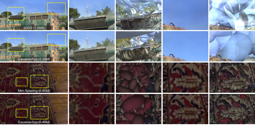
Figure 6: Visualization for rendered Gaussian ellipsoids. GaussianSpa adaptively reconstructs high-frequency (e.g., air outlet of the train, complex textures of the carpet) and low-frequency (e.g., large-area sky, simple textures of the carpet) regions using appropriate numbers of Gaussians, respectively, more precisely matching the original textures and shapes, compared to the state-of-the-art Mini-Splatting [20] and the vanilla 3DGS.

4.3 Visual Quality Results

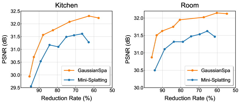
Figure 7: Quality-Reduction Rate curves on the (left) Kitchen and (right) Room scenes. GaussianSpa outperforms Mini-Splatting [20] across all reduction rates.

As depicted in Figure 5, we present the rendered images on the Drjohnson and Counter scenes [5, 23] for visual quality evaluation, in comparison to LightGaussian [19], Mini-Splattin [20], and the vanilla 3DGS. Together with Figure 1, those outcomes demonstrate the superior rendering quality of our GaussianSpa on diverse scenes over existing approaches, consistent with the quantitative results in the previous subsection. For instance, as shown in Figure 5, GaussianSpa accurately renders the outlet behind the railings for the Playroom scene, while LightGaussian [19] and Mini-Splatting [20] lose this object. Furthermore, GaussianSpa fully recovers the original details of the zoom-in object in the Counter scene, while other methods outcome blurry surfaces.

We comprehensively analyze the proposed GaussianSpa by visualizing the rendered Gaussian ellipsoids and final point clouds in Figure 6 and Figure 8, respectively. Those visualized results demonstrate that GaussianSpa can adaptively control the density to match the details when sparsifying the Gaussians, ensuring high-quality sparse 3D representation. From Figure 6, we can observe that GaussianSpa uses fewer but larger Gaussians to represent the blue sky and uses dense Gaussians to render complex carpet textures, providing precise rendering of details in the zoom-in images. In contrast, Mini-Splatting [20] cannot fully reconstruct the details, leading to blurry rendered textures. Figure 8 further demonstrates our superiority in simplification among existing approaches. GaussianSpa adaptively reduce the Gaussians in the low-frequency areas and preserve more Gaussians in high-frequency areas that generally need more Gaussians to synthesize, resulting in sparse Gaussian point clouds that precisely outline the scene contours.

5 Discussion

5.1 Convergence Analysis

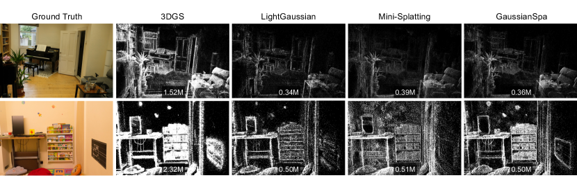
Figure 8: Visualized point clouds for the Room and Drjohnson scenes. The numbers of remaining Gaussians in millions are displayed. With GaussianSpa, sparse Gaussians concentrate on high-frequency areas after our “optimizing-sparsifying”-integrated training process, ensuring the capability to capture detail-rich textures and shapes. On the contrary, the point clouds produced by other approaches cannot outline the contours.

We analyze convergence behavior of the proposed GaussianSpa and appropriately set hyper-parameters, such as $\delta$, which controls the sparsity strength in Eq. 10. As introduced in Section 3, GaussianSpa performs the “sparsifying” step every fixed number of iterations, referred to here as “interval” here. We plot loss curves for multiple $\delta$’s and intervals in Figure 9. It is seen that with different $\delta$ and interval values, the curves converge well at a similar rate during our “optimizing-sparsifying”-integrated training process. After removing “zero” Gaussians at iteration 25K, the loss curve still exhibits a consistent convergence, confirming the feasibility of GaussianSpa.

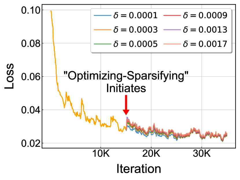
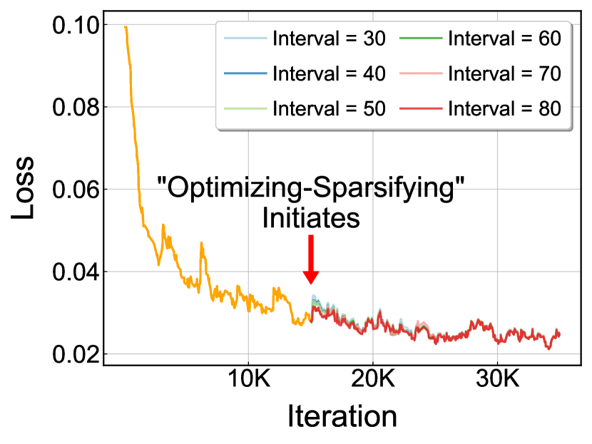
Figure 9: Loss curves with multiple (left) $\delta$ and (right) interval settings. The curves show that GaussianSpa exhibits a good convergence behaviour in the “optimizing-sparsifying”-integrated training process.

5.2 Generality of GaussianSpa

GaussianSpa is a general Gaussian simplification framework. Existing importance measurement criteria can be applied to project the auxiliary variable $\bm{z}$ onto the sparse space in the “sparsifying” step, Eq. 15, obtaining more compact 3DGS models with improved rendering quality. For example, we employ the criterion from LightGaussian [19] and plot the PSNR curves at multiple Gaussian reduction rates in Figure 13 in the Appendix. It is observed that GaussianSpa consistently outperforms LightGaussian [19] with an average of 0.4 dB improvement for the Playroom and Kitchen scenes.

5.3 Storage Compression

While GaussianSpa focuses on simplifying and optimizing the number of Gaussians to obtain a sparse 3DGS representation, existing compression techniques such as SH optimization and vector quantization can be applied as add-ons to the simplified 3DGS model. As shown in Table 2, we present the final storage cost for the Mip-NeRF 360 dataset by incorporating the SH distillation and vector quantization methods proposed by LightGaussian [19]. This comparison demonstrates that GaussianSpa can achieve the lowest storage consumption with additional compression techniques while maintaining superior rendering quality over existing hybrid compression methods, such as EfficientGS [31] and LightGaussian [19].

5.4 Relation to Other Optimization Algorithms

The “optimizing-sparsifying” algorithm in our proposed GaussianSpa can be categorized into the class of optimization algorithms that project the target variable onto a constrained space, specifically the $\ell_{p}$ ball (where $p=0$ in our case). This approach is similar to foundational optimization algorithms in compressed sensing [16] and sparse learning [9], such as Ridge regression [24] and Lasso regression [48]. These algorithms extend the least squares regression by incorporating $\ell_{p}$ regularization – Ridge regression adds the $\ell_{2}$ regularization, while the Lasso regression adds the $\ell_{1}$ regularization. The regularization acts as a penalty, combined with quadratic loss, reformulating the problem as a convex optimization task.

Method	PSNR↑	SSIM↑	LPIPS↓	Storage↓
EfficientGS [31]	27.38	0.817	0.216	98 MB
LightGaussian [19]	27.28	0.805	0.243	42 MB
GaussianSpa	27.85	0.825	0.214	25 MB

Table 2: Storage comparison evaluated on the Mip-NeRF 360 dataset. GaussianSpa’s storage cost is reported based on the add-on compression methods (i.e., SH distillation and vector quantization) from LightGaussian [19].

However, neither $\ell_{1}$ nor $\ell_{2}$ regularization yields truly sparse solutions; achieving genuine sparsity requires the $\ell_{0}$ regularization. Yet, when $p=0$, the problem, also known as the sparse coding problem [41], becomes nonconvex and is generally recognized as NP-hard [15, 37, 49]. This complexity makes it computationally impractical when the dimension of the target variable is high. In such cases, Lasso (where $p=1$) offers a convex constraint region, serving as the tightest convex surrogate for the sparse coding problem, albeit with some sacrifice in exact sparsity [11]. Another alternative solver suitable for this case is a greedy algorithm, such as the Matching Pursuit algorithm [33, 45]. However, this algorithm cannot guarantee the global optima.

Iterative thresholding (IT) is another direction to address this problem effectively [17, 14, 18]. These algorithms perform a matrix multiplication and its adjoint at each iteration, followed by a scalar shrinkage step, which yields a simple yet highly effective structure. Furthermore, a closed-form solution for the global minimizer of the sparse coding problem can be obtained – even for non-convex cases – under the condition that a unitary matrix is involved [17]. Inspired by this, we introduce a duplicated variable (i.e., $\bm{z}$) and project it onto the $\ell_{0}$ ball, optimizing over two variables alternately, similar to the alternating direction method of multipliers [8]. By leveraging the simplicity of the unitary case, the “sparsifying” step aligns with this scenario and thus admits an explicit solution. Hence, our algorithm simultaneously benefits from the sparsity imposed by the $\ell_{0}$ constraint and achieves fast convergence, guided by the explicit solution.

6 Conclusion

In this paper, we present an optimization-based 3DGS simplification framework, GaussianSpa, for compact and high-quality sparse view synthesis. GaussianSpa formulates 3DGS simplification as a constrained optimization problem with a sparsity constraint on the Gaussian opacities. Then, we propose an “optimizing-sparsifying” solution to efficiently solve the formulated problem during the 3DGS training process. We comprehensively evaluate the proposed GaussianSpa on multiple datasets with quantitative results and qualitative analyses, demonstrating the superiority in rendering quality with fewer Gaussians compared to existing state-of-the-art approaches.

Appendix

7 Additional Results

7.1 Additional Quantitative Results

We summarize additional quantitative results on the Mip-NeRF 360, Tanks&Temples, and Deep Blending datasets in Table 4, Table 5, and Table 3, respectively. We plot additional PSNR-#Gaussians curves on diverse Scenes in Figure 13, in comparison with Mini-Splatting [20] and LightGaussian [19]. It can be observed that with the same number of Gaussians, our GaussianSpa shows superior rendering outcomes.

7.2 Additional Visual Quality Results

Figure 10 and Figure 11 provide additional rendered images comparing GaussianSpa with LightGaussian [19], Mini-Splatting [20], and original 3DGS on various scenes. Those additional results demonstrate our GaussianSpa achieves stronger representational power for background and detail-rich areas such as walls, carpets, and ladders, showcasing superior rendering qualities. We also present additional point cloud views in Figure 12. This further illustrates that GaussianSpa creates a high-quality sparse 3D representation that adaptively uses more Gaussians to represent high-frequency areas.

Scene	Method	PSNR↑	SSIM↑	LPIPS↓	# G (M)↓
Drjohnson	3DGS	28.77	0.900	0.250	3.260
	Mini-Splatting	29.37	0.904	0.261	0.377
	GaussianSpa	29.89	0.913	0.243	0.450
	GaussianSpa	29.82	0.909	0.254	0.293
Playroom	3DGS	30.07	0.900	0.250	2.290
	Mini-Splatting	30.72	0.914	0.248	0.417
	GaussianSpa	30.84	0.916	0.254	0.219
	GaussianSpa	30.84	0.916	0.254	0.219
Average	3DGS	29.42	0.900	0.250	2.780
	Mini-Splatting	30.05	0.909	0.254	0.397
	GaussianSpa	30.37	0.914	0.249	0.335
	GaussianSpa	30.33	0.912	0.254	0.256

Table 3: Deep Blending per scene results. 3DGS results are reported from [22]. Mini-Splatting [20] results are replicated using official code.

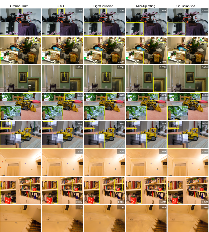
Figure 10: Additional visual comparison on more scenes. The numbers of remaining Gaussians in millions are displayed.

Figure 11: (Continue) Additional visual comparison on more scenes. The numbers of remaining Gaussians in millions are displayed.

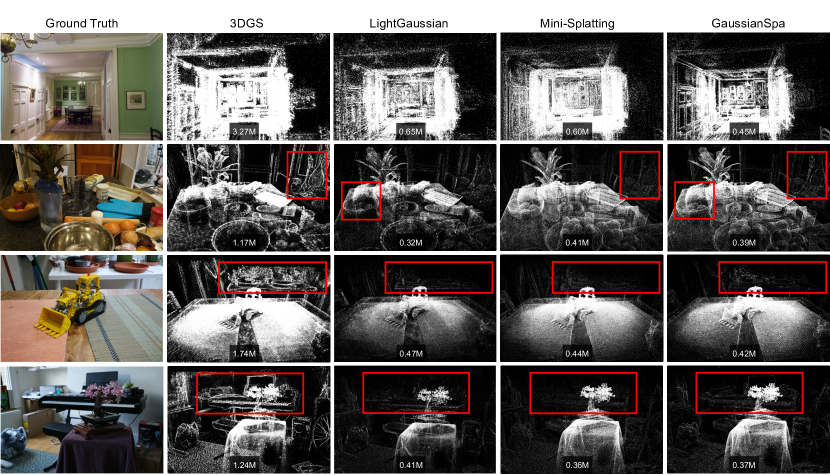
Figure 12: Additional visualized point clouds. The numbers of remaining Gaussians in millions are displayed.

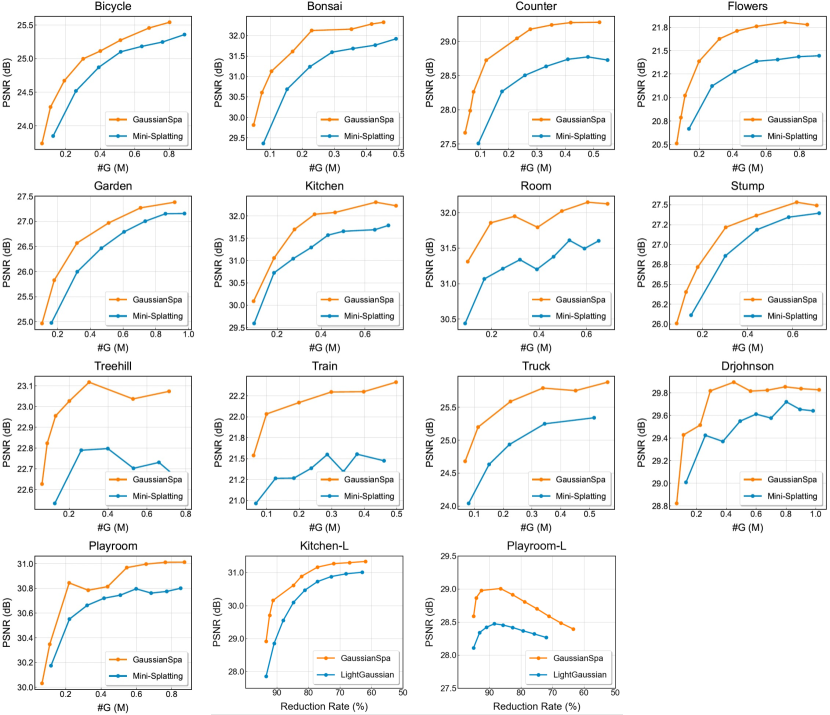
Figure 13: The first 13 sub-figures: Quality-#G (the number of Gaussians in millions) curves comparing GaussianSpa with Mini-Splatting [20] on multiple scenes. Our GaussianSpa consistently outperforms Mini-Splatting [20] with the same #G. The last two sub-figures: Quality-Reduction Rate curves comparing GaussianSpa with LightGaussian [19] on the Kitchen and Playroom scenes.

Scene	Method	PSNR↑	SSIM↑	LPIPS↓	# G (M)↓
Bicycle	3DGS	25.13	0.750	0.240	5.310
	Mini-Splatting	25.21	0.760	0.247	0.646
	GaussianSpa	25.44	0.769	0.246	0.656
Bonsai	3DGS	32.19	0.950	0.180	1.250
	Mini-Splatting	31.73	0.945	0.180	0.360
	GaussianSpa	32.40	0.947	0.174	0.372
Counter	3DGS	29.11	0.910	0.180	1.170
	Mini-Splatting	28.53	0.911	0.184	0.408
	GaussianSpa	29.23	0.919	0.176	0.392
Flowers	3DGS	21.37	0.590	0.360	3.470
	Mini-Splatting	21.42	0.616	0.336	0.670
	GaussianSpa	21.75	0.610	0.329	0.674
Garden	3DGS	27.32	0.860	0.120	5.690
	Mini-Splatting	26.99	0.842	0.156	0.738
	GaussianSpa	27.26	0.848	0.151	0.728
Kitchen	3DGS	31.53	0.930	0.120	1.770
	Mini-Splatting	31.24	0.929	0.122	0.438
	GaussianSpa	32.03	0.934	0.117	0.423
Room	3DGS	31.59	0.920	0.200	1.500
	Mini-Splatting	31.44	0.929	0.193	0.394
	GaussianSpa	32.04	0.933	0.188	0.355
Stump	3DGS	26.73	0.770	0.240	4.420
	Mini-Splatting	27.35	0.803	0.219	0.717
	GaussianSpa	27.56	0.808	0.218	0.690
Treehill	3DGS	22.61	0.640	0.350	3.420
	Mini-Splatting	22.69	0.652	0.332	0.663
	GaussianSpa	22.94	0.660	0.329	0.637
Average	3DGS	27.45	0.810	0.220	3.110
	Mini-Splatting	27.40	0.821	0.219	0.559
	GaussianSpa	27.85	0.825	0.214	0.547

Table 4: MiP-NeRF360 per scene results. 3DGS results are reported from [22]. Mini-Splatting [20] results are replicated using official code.

Scene	Method	PSNR↑	SSIM↑	LPIPS↓	# G (M)↓
Train	3DGS	21.94	0.810	0.200	1.110
	Mini-Splatting	21.78	0.805	0.231	0.287
	GaussianSpa	22.17	0.815	0.228	0.199
Truck	3DGS	25.31	0.880	0.150	2.540
	Mini-Splatting	25.13	0.878	0.141	0.352
	GaussianSpa	25.79	0.888	0.132	0.338
Average	3DGS	23.63	0.850	0.180	1.830
	Mini-Splatting	23.45	0.841	0.186	0.319
	GaussianSpa	23.98	0.852	0.180	0.269

Table 5: Tanks&Temples per scene results. 3DGS results are reported from [22]. Mini-Splatting [20] results are replicated using official code.

References

- Abadi et al. [2016] Martín Abadi, Paul Barham, Jianmin Chen, Zhifeng Chen, Andy Davis, Jeffrey Dean, Matthieu Devin, Sanjay Ghemawat, Geoffrey Irving, Michael Isard, et al. TensorFlow: a system for Large-Scale machine learning. In 12th USENIX symposium on operating systems design and implementation (OSDI 16), pages 265–283, 2016.
- Avidan and Shashua [1997] Shai Avidan and Amnon Shashua. Novel view synthesis in tensor space. In Proceedings of IEEE computer society conference on computer vision and pattern recognition, pages 1034–1040. IEEE, 1997.
- Barron et al. [2021] Jonathan T Barron, Ben Mildenhall, Matthew Tancik, Peter Hedman, Ricardo Martin-Brualla, and Pratul P Srinivasan. Mip-nerf: A multiscale representation for anti-aliasing neural radiance fields. In Proceedings of the IEEE/CVF international conference on computer vision, pages 5855–5864, 2021.
- Barron et al. [2022a] Jonathan T Barron, Ben Mildenhall, Dor Verbin, Pratul P Srinivasan, and Peter Hedman. Mip-nerf 360: Unbounded anti-aliased neural radiance fields. In Proceedings of the IEEE/CVF conference on computer vision and pattern recognition, pages 5470–5479, 2022a.
- Barron et al. [2022b] Jonathan T. Barron, Ben Mildenhall, Dor Verbin, Pratul P. Srinivasan, and Peter Hedman. Mip-nerf 360: Unbounded anti-aliased neural radiance fields. CVPR, 2022b.
- Barron et al. [2023] Jonathan T Barron, Ben Mildenhall, Dor Verbin, Pratul P Srinivasan, and Peter Hedman. Zip-nerf: Anti-aliased grid-based neural radiance fields. In Proceedings of the IEEE/CVF International Conference on Computer Vision, pages 19697–19705, 2023.
- Boyd and Vandenberghe [2004] Stephen Boyd and Lieven Vandenberghe. Convex optimization. Cambridge university press, 2004.
- Boyd et al. [2011] Stephen Boyd, Neal Parikh, Eric Chu, Borja Peleato, Jonathan Eckstein, et al. Distributed optimization and statistical learning via the alternating direction method of multipliers. Foundations and Trends® in Machine learning, 3(1):1–122, 2011.
- Bruckstein et al. [2009] Alfred M Bruckstein, David L Donoho, and Michael Elad. From sparse solutions of systems of equations to sparse modeling of signals and images. SIAM review, 51(1):34–81, 2009.
- Chen and Wang [2024] Guikun Chen and Wenguan Wang. A survey on 3d gaussian splatting. arXiv preprint arXiv:2401.03890, 2024.
- Chen et al. [2001] Scott Shaobing Chen, David L Donoho, and Michael A Saunders. Atomic decomposition by basis pursuit. SIAM review, 43(1):129–159, 2001.
- Chen et al. [2025] Yihang Chen, Qianyi Wu, Weiyao Lin, Mehrtash Harandi, and Jianfei Cai. Hac: Hash-grid assisted context for 3d gaussian splatting compression. In European Conference on Computer Vision, pages 422–438. Springer, 2025.
- Cheng et al. [2024] Kai Cheng, Xiaoxiao Long, Kaizhi Yang, Yao Yao, Wei Yin, Yuexin Ma, Wenping Wang, and Xuejin Chen. Gaussianpro: 3d gaussian splatting with progressive propagation. In Forty-first International Conference on Machine Learning, 2024.
- Daubechies et al. [2004] Ingrid Daubechies, Michel Defrise, and Christine De Mol. An iterative thresholding algorithm for linear inverse problems with a sparsity constraint. Communications on Pure and Applied Mathematics: A Journal Issued by the Courant Institute of Mathematical Sciences, 57(11):1413–1457, 2004.
- Davis [1994] Geoffrey Mark Davis. Adaptive nonlinear approximations. New York University, 1994.
- Donoho [2006] David L Donoho. Compressed sensing. IEEE Transactions on information theory, 52(4):1289–1306, 2006.
- Elad et al. [2007] Michael Elad, Boaz Matalon, Joseph Shtok, and Michael Zibulevsky. A wide-angle view at iterated shrinkage algorithms. In Wavelets XII, pages 15–33. SPIE, 2007.
- Eldar and Kutyniok [2012] Yonina C Eldar and Gitta Kutyniok. Compressed sensing: theory and applications. Cambridge university press, 2012.
- Fan et al. [2023] Zhiwen Fan, Kevin Wang, Kairun Wen, Zehao Zhu, Dejia Xu, and Zhangyang Wang. Lightgaussian: Unbounded 3d gaussian compression with 15x reduction and 200+ fps. arXiv preprint arXiv:2311.17245, 2023.
- Fang and Wang [2024] Guangchi Fang and Bing Wang. Mini-splatting: Representing scenes with a constrained number of gaussians. arXiv preprint arXiv:2403.14166, 2024.
- Gao et al. [2022] Kyle Gao, Yina Gao, Hongjie He, Dening Lu, Linlin Xu, and Jonathan Li. Nerf: Neural radiance field in 3d vision, a comprehensive review. arXiv preprint arXiv:2210.00379, 2022.
- Girish et al. [2023] Sharath Girish, Kamal Gupta, and Abhinav Shrivastava. Eagles: Efficient accelerated 3d gaussians with lightweight encodings. arXiv preprint arXiv:2312.04564, 2023.
- Hedman et al. [2018] Peter Hedman, Julien Philip, True Price, Jan-Michael Frahm, George Drettakis, and Gabriel Brostow. Deep blending for free-viewpoint image-based rendering. ACM Transactions on Graphics (ToG), 37(6):1–15, 2018.
- Hoerl and Kennard [1970] Arthur E Hoerl and Robert W Kennard. Ridge regression: Biased estimation for nonorthogonal problems. Technometrics, 12(1):55–67, 1970.
- Kerbl et al. [2023] Bernhard Kerbl, Georgios Kopanas, Thomas Leimkühler, and George Drettakis. 3d gaussian splatting for real-time radiance field rendering. ACM Trans. Graph., 42(4):139–1, 2023.
- Kim et al. [2024] Sieun Kim, Kyungjin Lee, and Youngki Lee. Color-cued efficient densification method for 3d gaussian splatting. In Proceedings of the IEEE/CVF Conference on Computer Vision and Pattern Recognition, pages 775–783, 2024.
- Knapitsch et al. [2017] Arno Knapitsch, Jaesik Park, Qian-Yi Zhou, and Vladlen Koltun. Tanks and temples: Benchmarking large-scale scene reconstruction. ACM Transactions on Graphics, 36(4), 2017.
- Kopanas et al. [2021] Georgios Kopanas, Julien Philip, Thomas Leimkühler, and George Drettakis. Point-based neural rendering with per-view optimization. In Computer Graphics Forum, pages 29–43. Wiley Online Library, 2021.
- Lee et al. [2024] Joo Chan Lee, Daniel Rho, Xiangyu Sun, Jong Hwan Ko, and Eunbyung Park. Compact 3d gaussian representation for radiance field. In Proceedings of the IEEE/CVF Conference on Computer Vision and Pattern Recognition, pages 21719–21728, 2024.
- Liu et al. [2024a] Rong Liu, Rui Xu, Yue Hu, Meida Chen, and Andrew Feng. Atomgs: Atomizing gaussian splatting for high-fidelity radiance field. arXiv preprint arXiv:2405.12369, 2024a.
- Liu et al. [2024b] Wenkai Liu, Tao Guan, Bin Zhu, Lili Ju, Zikai Song, Dan Li, Yuesong Wang, and Wei Yang. Efficientgs: Streamlining gaussian splatting for large-scale high-resolution scene representation. arXiv preprint arXiv:2404.12777, 2024b.
- Lu et al. [2024] Tao Lu, Mulin Yu, Linning Xu, Yuanbo Xiangli, Limin Wang, Dahua Lin, and Bo Dai. Scaffold-gs: Structured 3d gaussians for view-adaptive rendering. In Proceedings of the IEEE/CVF Conference on Computer Vision and Pattern Recognition, pages 20654–20664, 2024.
- Mallat and Zhang [1993] Stéphane G Mallat and Zhifeng Zhang. Matching pursuits with time-frequency dictionaries. IEEE Transactions on signal processing, 41(12):3397–3415, 1993.
- Mallick et al. [2024] Saswat Subhajyoti Mallick, Rahul Goel, Bernhard Kerbl, Francisco Vicente Carrasco, Markus Steinberger, and Fernando De La Torre. Taming 3dgs: High-quality radiance fields with limited resources. arXiv preprint arXiv:2406.15643, 2024.
- Mildenhall et al. [2021] Ben Mildenhall, Pratul P Srinivasan, Matthew Tancik, Jonathan T Barron, Ravi Ramamoorthi, and Ren Ng. Nerf: Representing scenes as neural radiance fields for view synthesis. Communications of the ACM, 65(1):99–106, 2021.
- Morgenstern et al. [2023] Wieland Morgenstern, Florian Barthel, Anna Hilsmann, and Peter Eisert. Compact 3d scene representation via self-organizing gaussian grids. arXiv preprint arXiv:2312.13299, 2023.
- Natarajan [1995] Balas Kausik Natarajan. Sparse approximate solutions to linear systems. SIAM journal on computing, 24(2):227–234, 1995.
- Navaneet et al. [2024] KL Navaneet, Kossar Pourahmadi Meibodi, Soroush Abbasi Koohpayegani, and Hamed Pirsiavash. Compgs: Smaller and faster gaussian splatting with vector quantization. In European Conference on Computer Vision, 2024.
- Niedermayr et al. [2024] Simon Niedermayr, Josef Stumpfegger, and Rüdiger Westermann. Compressed 3d gaussian splatting for accelerated novel view synthesis. In Proceedings of the IEEE/CVF Conference on Computer Vision and Pattern Recognition, pages 10349–10358, 2024.
- Niemeyer et al. [2024] Michael Niemeyer, Fabian Manhardt, Marie-Julie Rakotosaona, Michael Oechsle, Daniel Duckworth, Rama Gosula, Keisuke Tateno, John Bates, Dominik Kaeser, and Federico Tombari. Radsplat: Radiance field-informed gaussian splatting for robust real-time rendering with 900+ fps. arXiv preprint arXiv:2403.13806, 2024.
- Oktar and Turkan [2018] Yigit Oktar and Mehmet Turkan. A review of sparsity-based clustering methods. Signal processing, 148:20–30, 2018.
- Papantonakis et al. [2024] Panagiotis Papantonakis, Georgios Kopanas, Bernhard Kerbl, Alexandre Lanvin, and George Drettakis. Reducing the memory footprint of 3d gaussian splatting. Proceedings of the ACM on Computer Graphics and Interactive Techniques, 7(1):1–17, 2024.
- Parikh et al. [2014] Neal Parikh, Stephen Boyd, et al. Proximal algorithms. Foundations and trends® in Optimization, 1(3):127–239, 2014.
- Paszke et al. [2019] Adam Paszke, Sam Gross, Francisco Massa, Adam Lerer, James Bradbury, Gregory Chanan, Trevor Killeen, Zeming Lin, Natalia Gimelshein, Luca Antiga, et al. Pytorch: An imperative style, high-performance deep learning library. Advances in neural information processing systems, 32, 2019.
- Pati et al. [1993] Yagyensh Chandra Pati, Ramin Rezaiifar, and Perinkulam Sambamurthy Krishnaprasad. Orthogonal matching pursuit: Recursive function approximation with applications to wavelet decomposition. In Proceedings of 27th Asilomar conference on signals, systems and computers, pages 40–44. IEEE, 1993.
- Ren et al. [2024] Kerui Ren, Lihan Jiang, Tao Lu, Mulin Yu, Linning Xu, Zhangkai Ni, and Bo Dai. Octree-gs: Towards consistent real-time rendering with lod-structured 3d gaussians. arXiv preprint arXiv:2403.17898, 2024.
- Schonberger and Frahm [2016] Johannes L Schonberger and Jan-Michael Frahm. Structure-from-motion revisited. In Proceedings of the IEEE conference on computer vision and pattern recognition, pages 4104–4113, 2016.
- Tibshirani [1996] Robert Tibshirani. Regression shrinkage and selection via the lasso. Journal of the Royal Statistical Society Series B: Statistical Methodology, 58(1):267–288, 1996.
- Tillmann [2014] Andreas M Tillmann. On the computational intractability of exact and approximate dictionary learning. IEEE Signal Processing Letters, 22(1):45–49, 2014.
- Van Den Oord et al. [2017] Aaron Van Den Oord, Oriol Vinyals, et al. Neural discrete representation learning. Advances in neural information processing systems, 30, 2017.
- Wang et al. [2024] Henan Wang, Hanxin Zhu, Tianyu He, Runsen Feng, Jiajun Deng, Jiang Bian, and Zhibo Chen. End-to-end rate-distortion optimized 3d gaussian representation. arXiv preprint arXiv:2406.01597, 2024.
- Xie et al. [2024] Shuzhao Xie, Weixiang Zhang, Chen Tang, Yunpeng Bai, Rongwei Lu, Shijia Ge, and Zhi Wang. Mesongs: Post-training compression of 3d gaussians via efficient attribute transformation. arXiv preprint arXiv:2409.09756, 2024.
- Yang et al. [2024] Runyi Yang, Zhenxin Zhu, Zhou Jiang, Baijun Ye, Xiaoxue Chen, Yifei Zhang, Yuantao Chen, Jian Zhao, and Hao Zhao. Spectrally pruned gaussian fields with neural compensation. arXiv preprint arXiv:2405.00676, 2024.
- Zhang et al. [2024] Zhaoliang Zhang, Tianchen Song, Yongjae Lee, Li Yang, Cheng Peng, Rama Chellappa, and Deliang Fan. Lp-3dgs: Learning to prune 3d gaussian splatting. arXiv preprint arXiv:2405.18784, 2024.
- Zwicker et al. [2001] M. Zwicker, H. Pfister, J. van Baar, and M. Gross. Ewa volume splatting. In Proceedings Visualization, 2001. VIS ’01., pages 29–538, 2001.