Real randomized measurements for analyzing properties of quantum states
Jin-Min Liang
State Key Laboratory for Mesoscopic Physics, School of Physics, Frontiers Science Center for Nano-optoelectronics, Peking University, Beijing 100871, China
Satoya Imai
satoyaimai@yahoo.co.jp
QSTAR, INO-CNR, and LENS, Largo Enrico Fermi, 2, 50125 Firenze, Italy
Shuheng Liu
State Key Laboratory for Mesoscopic Physics, School of Physics, Frontiers Science Center for Nano-optoelectronics, Peking University, Beijing 100871, China
Shao-Ming Fei
School of Mathematical Sciences, Capital Normal University, Beijing 100048, China
Otfried Gühne
Naturwissenschaftlich-Technische Fakultät, Universität Siegen, Walter-Flex-Straße 3, 57068 Siegen, Germany
Qiongyi He
qiongyihe@pku.edu.cn
State Key Laboratory for Mesoscopic Physics, School of Physics, Frontiers Science Center for Nano-optoelectronics, Peking University, Beijing 100871, China
Collaborative Innovation Center of Extreme Optics, Shanxi University, Taiyuan, Shanxi 030006, China
Hefei National Laboratory, Hefei 230088, China
(December 5, 2024 )
Abstract
Randomized measurements are useful for analyzing quantum systems especially when quantum control is not fully perfect. However, their practical realization typically requires multiple rotations in the complex space due to the adoption of random unitaries. Here, we introduce two simplified randomized measurements that limit rotations in a subspace of the complex space. The first is real randomized measurements (RRMs) with orthogonal evolution and real local observables. The second is partial real randomized measurements (PRRMs) with orthogonal evolution and imaginary local observables. We show that these measurement protocols exhibit different abilities in capturing correlations of bipartite systems. We explore various applications of RRMs and PRRMs in different quantum information tasks such as characterizing high-dimensional entanglement, quantum imaginarity, and predicting properties of quantum states with classical shadow.
Introduction.— Recent experimental progress in controlling and manipulating larger quantum systems has enabled quantum advantages beyond classical regimes [1 , 2 , 3 ] . Extracting useful quantum information via measurements is essential for characterizing and analyzing large quantum systems. However, the curse of dimensionality poses challenges in reconstructing large density matrices by state tomography [4 , 5 ] . Although several computationally and experimentally efficient tomography methods have been designed [6 , 7 , 8 , 9 , 10 , 11 ] , these methods either still require complex optimization or are limited to specific states.
A feasible strategy is randomized measurements (RMs), which rotate measurement directions arbitrarily on each subsystem and collect measured data to analyze the properties of quantum states [12 , 13 ] . Applications have emerged in various domains, including quantum simulation [14 , 15 ] , state overlaps [16 , 17 , 18 ] , classical shadow tomography [19 , 20 ] , and the estimation of Rényi entropies [21 , 22 , 23 ] , partial transpose moments [24 , 25 , 26 , 27 , 28 ] , and quantum Fisher information [29 , 30 , 31 ] .
In RMs, Alice and Bob apply local random unitaries U A ⊗ U B tensor-product subscript 𝑈 𝐴 subscript 𝑈 𝐵 U_{A}\otimes U_{B} ϱ italic-ϱ \varrho M A ⊗ M B tensor-product subscript 𝑀 𝐴 subscript 𝑀 𝐵 M_{A}\otimes M_{B} 𝐔 ( d ) 𝐔 𝑑 \bm{\mathrm{U}}(d) t 𝑡 t
R A B ( t ) = ∫ 𝑑 U A ∫ 𝑑 U B [ tr ( ϱ U A M A U A † ⊗ U B M B U B † ) ] t . superscript subscript 𝑅 𝐴 𝐵 𝑡 differential-d subscript 𝑈 𝐴 differential-d subscript 𝑈 𝐵 superscript delimited-[] tr tensor-product italic-ϱ subscript 𝑈 𝐴 subscript 𝑀 𝐴 superscript subscript 𝑈 𝐴 † subscript 𝑈 𝐵 subscript 𝑀 𝐵 superscript subscript 𝑈 𝐵 † 𝑡 R_{AB}^{(t)}\!=\!\!\int\!dU_{A}\!\!\int\!dU_{B}\,[{\mathrm{tr}}(\varrho U_{A}M_{A}U_{A}^{{\dagger}}\otimes U_{B}M_{B}U_{B}^{{\dagger}})]^{t}. (1)
These moments provide an approach to characterize the quantum entanglement [32 , 33 , 34 ] . The techniques have been extended to high-dimensional systems [35 , 36 , 37 ] and multiqubit systems [38 , 39 , 40 ] .
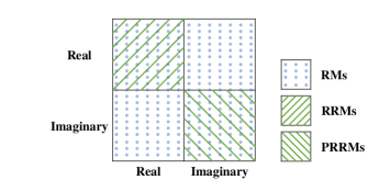
Figure 1: Layout for characterizing the correlations of bipartite quantum states from randomized measurements (RMs), real randomized measurements (RRMs), and partial real randomized measurements (PRRMs), respectively, as given by Eqs. (1 2 3 1
Although RMs are effective tools for analyzing quantum states, they still face several challenges. First, the practical implementation of RMs often requires multiple rotations in the whole complex space by successive tuning d 2 − 1 superscript 𝑑 2 1 d^{2}-1 d 𝑑 d [41 , 42 ] with certain symmetries like time-reversal symmetry [43 , 44 , 45 , 46 ] , employing RMs designed for the complex full space as in Eq. (1 [47 ] . Finally, the moments in Eq. (1 1 [48 , 49 , 50 , 51 , 52 , 53 ] .
In this paper, we generalize standard RMs to address these issues. In the following, we call a Hermitian operator X 𝑋 X X = X ⊤ 𝑋 superscript 𝑋 top X=X^{\top} X = − X ⊤ 𝑋 superscript 𝑋 top X=-X^{\top} ⊤ top \top
Assumptions .
(i) The random unitaries of the form U = e i θ O 𝑈 superscript 𝑒 𝑖 𝜃 𝑂 U=e^{i\theta}O θ ∈ [ 0 , 2 π ) 𝜃 0 2 𝜋 \theta\in[0,2\pi) O 𝑂 O O O ⊤ = O ⊤ O = 𝟙 𝑂 superscript 𝑂 top superscript 𝑂 top 𝑂 1 OO^{\top}=O^{\top}O=\mathbbm{1} M A subscript 𝑀 𝐴 M_{A} M B subscript 𝑀 𝐵 M_{B} M A subscript 𝑀 𝐴 M_{A} M B subscript 𝑀 𝐵 M_{B}
Here we call RMs real randomized measurements (RRMs) if the RMs meet the conditions (i) and (ii) in Assumptions, and partial real randomized measurements (PRRMs) if the RMs meet (i) and (iii). First, we define the t 𝑡 t d 2 − 1 superscript 𝑑 2 1 d^{2}-1 L = ( d − 1 ) ( d + 2 ) / 2 𝐿 𝑑 1 𝑑 2 2 L=(d-1)(d+2)/2 L ^ = d ( d − 1 ) / 2 ^ 𝐿 𝑑 𝑑 1 2 \hat{L}=d(d-1)/2 [54 , 55 ] and the Schmidt dimensionality [56 , 57 , 58 ] . Moreover, we characterize the imaginarity of quantum states by combining RMs, RRMs, and PRRMs, accessing its lower bound for the existing measure [48 ] . Finally, we apply RRMs to classical shadow tomography [59 , 60 ] .
Real randomized measurements.— Suppose that Alice and Bob share a two-qudit state ϱ italic-ϱ \varrho O A subscript 𝑂 𝐴 O_{A} O B subscript 𝑂 𝐵 O_{B} 𝐎 ( d ) 𝐎 𝑑 \bm{\mathrm{O}}(d) M A subscript 𝑀 𝐴 M_{A} M B subscript 𝑀 𝐵 M_{B} M ^ A subscript ^ 𝑀 𝐴 \hat{M}_{A} M ^ B subscript ^ 𝑀 𝐵 \hat{M}_{B} □ ^ ^ □ \hat{\square} t 𝑡 t
Q A B ( t ) superscript subscript 𝑄 𝐴 𝐵 𝑡 \displaystyle Q_{AB}^{(t)}\! = ∫ 𝑑 O A ∫ 𝑑 O B [ tr ( ϱ O A M A O A ⊤ ⊗ O B M B O B ⊤ ) ] t , absent differential-d subscript 𝑂 𝐴 differential-d subscript 𝑂 𝐵 superscript delimited-[] tr tensor-product italic-ϱ subscript 𝑂 𝐴 subscript 𝑀 𝐴 superscript subscript 𝑂 𝐴 top subscript 𝑂 𝐵 subscript 𝑀 𝐵 superscript subscript 𝑂 𝐵 top 𝑡 \displaystyle=\!\!\int\!dO_{A}\!\!\int\!dO_{B}\,[{\mathrm{tr}}(\varrho O_{A}M_{A}O_{A}^{\top}\otimes O_{B}M_{B}O_{B}^{\top})]^{t}, (2)
Q ^ A B ( t ) superscript subscript ^ 𝑄 𝐴 𝐵 𝑡 \displaystyle\hat{Q}_{AB}^{(t)}\! = ∫ 𝑑 O A ∫ 𝑑 O B [ tr ( ϱ O A M ^ A O A ⊤ ⊗ O B M ^ B O B ⊤ ) ] t . absent differential-d subscript 𝑂 𝐴 differential-d subscript 𝑂 𝐵 superscript delimited-[] tr tensor-product italic-ϱ subscript 𝑂 𝐴 subscript ^ 𝑀 𝐴 superscript subscript 𝑂 𝐴 top subscript 𝑂 𝐵 subscript ^ 𝑀 𝐵 superscript subscript 𝑂 𝐵 top 𝑡 \displaystyle=\!\!\int\!dO_{A}\!\!\int\!dO_{B}\,[{\mathrm{tr}}(\varrho O_{A}\hat{M}_{A}O_{A}^{\top}\otimes O_{B}\hat{M}_{B}O_{B}^{\top})]^{t}. (3)
Note that the moments Q A B ( t ) superscript subscript 𝑄 𝐴 𝐵 𝑡 Q_{AB}^{(t)} Q ^ A B ( t ) superscript subscript ^ 𝑄 𝐴 𝐵 𝑡 \hat{Q}_{AB}^{(t)} R A B ( t ) superscript subscript 𝑅 𝐴 𝐵 𝑡 R_{AB}^{(t)} Q A B ( t ) ( ϱ ) = Q A B ( t ) ( W A ⊗ W B ϱ W A ⊤ ⊗ W B ⊤ ) superscript subscript 𝑄 𝐴 𝐵 𝑡 italic-ϱ superscript subscript 𝑄 𝐴 𝐵 𝑡 tensor-product tensor-product subscript 𝑊 𝐴 subscript 𝑊 𝐵 italic-ϱ superscript subscript 𝑊 𝐴 top superscript subscript 𝑊 𝐵 top Q_{AB}^{(t)}(\varrho)=Q_{AB}^{(t)}(W_{A}\otimes W_{B}\varrho W_{A}^{\top}\otimes W_{B}^{\top}) W A , W B ∈ 𝐎 ( d ) subscript 𝑊 𝐴 subscript 𝑊 𝐵
𝐎 𝑑 W_{A},W_{B}\in\bm{\mathrm{O}}(d) Q ^ A B ( t ) superscript subscript ^ 𝑄 𝐴 𝐵 𝑡 \hat{Q}_{AB}^{(t)} R A B ( t ) ( ϱ ) = R A B ( t ) ( V A ⊗ V B ϱ V A † ⊗ V B † ) superscript subscript 𝑅 𝐴 𝐵 𝑡 italic-ϱ superscript subscript 𝑅 𝐴 𝐵 𝑡 tensor-product tensor-product subscript 𝑉 𝐴 subscript 𝑉 𝐵 italic-ϱ superscript subscript 𝑉 𝐴 † superscript subscript 𝑉 𝐵 † R_{AB}^{(t)}(\varrho)=R_{AB}^{(t)}(V_{A}\otimes V_{B}\varrho V_{A}^{{\dagger}}\otimes V_{B}^{{\dagger}}) V A , V B ∈ 𝐔 ( d ) subscript 𝑉 𝐴 subscript 𝑉 𝐵
𝐔 𝑑 V_{A},V_{B}\in\bm{\mathrm{U}}(d) Q A B ( t ) superscript subscript 𝑄 𝐴 𝐵 𝑡 Q_{AB}^{(t)} Q ^ A B ( t ) superscript subscript ^ 𝑄 𝐴 𝐵 𝑡 \hat{Q}_{AB}^{(t)} [61 , 62 ] .
Let us discuss the difference among RMs, RRMs, and RRMs. Recall that any two-qudit state ϱ italic-ϱ \varrho
ϱ = 1 d 2 ∑ j , k = 0 d 2 − 1 T j k λ j ⊗ λ k , italic-ϱ 1 superscript 𝑑 2 superscript subscript 𝑗 𝑘
0 superscript 𝑑 2 1 tensor-product subscript 𝑇 𝑗 𝑘 subscript 𝜆 𝑗 subscript 𝜆 𝑘 \varrho=\frac{1}{d^{2}}\sum_{j,k=0}^{d^{2}-1}T_{jk}\lambda_{j}\otimes\lambda_{k}, (4)
where λ 0 = 𝟙 d subscript 𝜆 0 subscript 1 𝑑 \lambda_{0}=\mathbbm{1}_{d} d 𝑑 d λ j subscript 𝜆 𝑗 \lambda_{j} λ j = λ j † subscript 𝜆 𝑗 superscript subscript 𝜆 𝑗 † \lambda_{j}=\lambda_{j}^{{\dagger}} tr ( λ j λ k ) = d δ j k tr subscript 𝜆 𝑗 subscript 𝜆 𝑘 𝑑 subscript 𝛿 𝑗 𝑘 {\mathrm{tr}}(\lambda_{j}\lambda_{k})=d\delta_{jk} tr ( λ j ) = 0 tr subscript 𝜆 𝑗 0 {\mathrm{tr}}(\lambda_{j})=0 j > 0 𝑗 0 j>0 [63 , 64 ] . Note that each of ( d 2 − 1 ) superscript 𝑑 2 1 (d^{2}-1) Real GGMs consisting of L 𝐿 L λ j ⊤ = λ j superscript subscript 𝜆 𝑗 top subscript 𝜆 𝑗 \lambda_{j}^{\top}=\lambda_{j} Imaginary GGMs consisting of L ^ ^ 𝐿 \hat{L} λ j ⊤ = − λ j superscript subscript 𝜆 𝑗 top subscript 𝜆 𝑗 \lambda_{j}^{\top}=-\lambda_{j} L = ( d − 1 ) ( d + 2 ) / 2 𝐿 𝑑 1 𝑑 2 2 L=(d-1)(d+2)/2 L ^ = d ( d − 1 ) / 2 ^ 𝐿 𝑑 𝑑 1 2 \hat{L}=d(d-1)/2 L + L ^ = d 2 − 1 𝐿 ^ 𝐿 superscript 𝑑 2 1 L+\hat{L}=d^{2}-1 A
The bipartite correlations in ϱ italic-ϱ \varrho 1
Observation 1 .
The RMs given by Eq.(1 ϱ italic-ϱ \varrho 2 3 ϱ italic-ϱ \varrho 1 ϱ italic-ϱ \varrho
Q A B ( t ) ( ϱ ) + Q ^ A B ( t ) ( ϱ ) ≤ R A B ( t ) ( ϱ ) , ∀ ϱ , superscript subscript 𝑄 𝐴 𝐵 𝑡 italic-ϱ superscript subscript ^ 𝑄 𝐴 𝐵 𝑡 italic-ϱ superscript subscript 𝑅 𝐴 𝐵 𝑡 italic-ϱ for-all italic-ϱ
Q_{AB}^{(t)}(\varrho)+\hat{Q}_{AB}^{(t)}(\varrho)\leq R_{AB}^{(t)}(\varrho),\quad\forall\varrho, (5)
where the equality is attained when ϱ italic-ϱ \varrho ϱ = ϱ ⊤ italic-ϱ superscript italic-ϱ top \varrho=\varrho^{\top}
The proof of the Observation 1 B t = 2 𝑡 2 t=2 𝟙 d ⊗ 𝟙 d tensor-product subscript 1 𝑑 subscript 1 𝑑 \mathbbm{1}_{d}\otimes\mathbbm{1}_{d} 𝕊 = ∑ j , k | j k ⟩ ⟨ k j | 𝕊 subscript 𝑗 𝑘
ket 𝑗 𝑘 bra 𝑘 𝑗 \mathbb{S}=\sum_{j,k}|jk\rangle\langle kj| Π = ∑ j , k | j j ⟩ ⟨ k k | Π subscript 𝑗 𝑘
ket 𝑗 𝑗 bra 𝑘 𝑘 \Pi=\sum_{j,k}|jj\rangle\langle kk| [65 , 66 , 67 , 68 , 69 ] and Appendix A { | j ⟩ } ket 𝑗 \{|j\rangle\} d 𝑑 d
∫ 𝑑 U U ⊗ 2 𝒜 U † ⊗ 2 = α 𝟙 d ⊗ 𝟙 d + β 𝕊 , differential-d 𝑈 superscript 𝑈 tensor-product absent 2 𝒜 superscript 𝑈 † tensor-product absent 2
tensor-product 𝛼 subscript 1 𝑑 subscript 1 𝑑 𝛽 𝕊 \displaystyle\int dU\,U^{\otimes 2}\mathcal{A}U^{{\dagger}\otimes 2}=\alpha\mathbbm{1}_{d}\otimes\mathbbm{1}_{d}+\beta\mathbb{S}, (6)
∫ 𝑑 O O ⊗ 2 𝒜 O ⊤ ⊗ 2 = γ 1 𝟙 d ⊗ 𝟙 d + γ 2 𝕊 + γ 3 Π , differential-d 𝑂 superscript 𝑂 tensor-product absent 2 𝒜 superscript 𝑂 top tensor-product absent 2
tensor-product subscript 𝛾 1 subscript 1 𝑑 subscript 1 𝑑 subscript 𝛾 2 𝕊 subscript 𝛾 3 Π \displaystyle\int dO\,O^{\otimes 2}\mathcal{A}O^{\top\otimes 2}=\gamma_{1}\mathbbm{1}_{d}\otimes\mathbbm{1}_{d}+\gamma_{2}\mathbb{S}+\gamma_{3}\Pi, (7)
where the parameters α , β , γ 1 , γ 2 𝛼 𝛽 subscript 𝛾 1 subscript 𝛾 2
\alpha,\beta,\gamma_{1},\gamma_{2} γ 3 subscript 𝛾 3 \gamma_{3} 𝒜 𝒜 \mathcal{A} A 6 Π Π \Pi 7 ϱ italic-ϱ \varrho
Entanglement detection via RRMs. —We here employ RRMs to characterize high-dimensional bipartite entanglement. Recall that the so-called Schmidt number (SN) of ϱ italic-ϱ \varrho | ψ j ⟩ ket subscript 𝜓 𝑗 |\psi_{j}\rangle [56 ] , SN ( ϱ ) = min { r : ϱ = ∑ j p j | ψ j ⟩ ⟨ ψ j | , SR ( | ψ j ⟩ ) ≤ r } SN italic-ϱ : 𝑟 formulae-sequence italic-ϱ subscript 𝑗 subscript 𝑝 𝑗 ket subscript 𝜓 𝑗 bra subscript 𝜓 𝑗 SR ket subscript 𝜓 𝑗 𝑟 \textrm{SN}(\varrho)=\min\{r:\varrho=\sum_{j}p_{j}|\psi_{j}\rangle\langle\psi_{j}|,\textrm{SR}(|\psi_{j}\rangle)\leq r\} p j ≥ 0 subscript 𝑝 𝑗 0 p_{j}\geq 0 ∑ j p j = 1 subscript 𝑗 subscript 𝑝 𝑗 1 \sum_{j}p_{j}=1 ( ϱ ) italic-ϱ (\varrho)
The first step is to evaluate the orthogonal integrals of the moments Q A B ( t ) ( ϱ ) superscript subscript 𝑄 𝐴 𝐵 𝑡 italic-ϱ Q_{AB}^{(t)}(\varrho) 2 t = 2 , 4 𝑡 2 4
t=2,4 C
Q A B ( 2 ) superscript subscript 𝑄 𝐴 𝐵 2 \displaystyle Q_{AB}^{(2)} = 1 L 2 ∑ j = 1 L τ j 2 , absent 1 superscript 𝐿 2 superscript subscript 𝑗 1 𝐿 superscript subscript 𝜏 𝑗 2 \displaystyle=\frac{1}{L^{2}}\sum_{j=1}^{L}\tau_{j}^{2}, (8)
Q A B ( 4 ) superscript subscript 𝑄 𝐴 𝐵 4 \displaystyle Q_{AB}^{(4)} = W [ 2 ∑ j = 1 L τ j 4 + L 4 ( Q A B ( 2 ) ) 2 ] , absent 𝑊 delimited-[] 2 superscript subscript 𝑗 1 𝐿 superscript subscript 𝜏 𝑗 4 superscript 𝐿 4 superscript superscript subscript 𝑄 𝐴 𝐵 2 2 \displaystyle=W\left[2\sum_{j=1}^{L}\tau_{j}^{4}+L^{4}\left(Q_{AB}^{(2)}\right)^{2}\right], (9)
where τ j subscript 𝜏 𝑗 \tau_{j} T R = ( T j , k ) subscript 𝑇 𝑅 subscript 𝑇 𝑗 𝑘
T_{R}=(T_{j,k}) 4 j , k > 0 𝑗 𝑘
0 j,k>0 L = ( d − 1 ) ( d + 2 ) / 2 𝐿 𝑑 1 𝑑 2 2 L=(d-1)(d+2)/2 W = 3 Γ 2 ( L 2 ) 16 Γ 2 ( L + 4 2 ) 𝑊 3 superscript Γ 2 𝐿 2 16 superscript Γ 2 𝐿 4 2 W=\frac{3\Gamma^{2}(\frac{L}{2})}{16\Gamma^{2}\left(\frac{L+4}{2}\right)} Γ ( z ) Γ 𝑧 \Gamma(z) Γ ( z ) = ( z − 1 ) ! Γ 𝑧 𝑧 1 \Gamma(z)=(z-1)! z 𝑧 z [70 ] .
It is important to note that for higher-order moments, not all observables give rise to the same results, since orthogonal matrices do not imply sphere rotations, due to the lack of the Bloch sphere for d > 2 𝑑 2 d>2 8 9 t = 2 , 4 𝑡 2 4
t=2,4 d 𝑑 d [35 , 37 ] , for details see Appendix C d = 3 𝑑 3 d=3 M A = M B = diag ( 3 / 2 , 0 , − 3 / 2 ) subscript 𝑀 𝐴 subscript 𝑀 𝐵 diag 3 2 0 3 2 M_{A}=M_{B}=\mathrm{diag}(\sqrt{3/2},0,-\sqrt{3/2}) [37 ] .
Next, we propose our entanglement dimensionality criterion by adopting the second and fourth moments of RRMs. Our approach to detect SN( ϱ ) italic-ϱ (\varrho) ( Q A B ( 2 ) , Q A B ( 4 ) ) superscript subscript 𝑄 𝐴 𝐵 2 superscript subscript 𝑄 𝐴 𝐵 4 (Q_{AB}^{(2)},Q_{AB}^{(4)}) 8 9 [34 , 35 , 37 , 36 ] . The task is to obtain the lower boundary on this plane, so as to reveal a hierarchy of Schmidt numbers. To do so, we use the criterion [37 , 36 ] that any bipartite quantum state ϱ italic-ϱ \varrho SN ( ϱ ) ≤ r SN italic-ϱ 𝑟 \textrm{SN}(\varrho)\leq r ‖ T ‖ tr = ∑ j = 1 d 2 − 1 τ j ≤ r d − 1 subscript norm 𝑇 tr superscript subscript 𝑗 1 superscript 𝑑 2 1 subscript 𝜏 𝑗 𝑟 𝑑 1 \|T\|_{{\mathrm{tr}}}=\sum_{j=1}^{d^{2}-1}\tau_{j}\leq rd-1 r = 1 , ⋯ , d 𝑟 1 ⋯ 𝑑
r=1,\cdots,d ∥ ⋅ ∥ tr \|\cdot\|_{{\mathrm{tr}}} T 𝑇 T 4 r = 1 𝑟 1 r=1 [71 ] . Recalling that T R subscript 𝑇 𝑅 T_{R} T 𝑇 T ‖ T R ‖ tr = ∑ j = 1 L τ j ≤ r d − 1 subscript norm subscript 𝑇 R tr superscript subscript 𝑗 1 𝐿 subscript 𝜏 𝑗 𝑟 𝑑 1 \|T_{\mathrm{R}}\|_{{\mathrm{tr}}}=\sum_{j=1}^{L}\tau_{j}\leq rd-1 [72 ] . We summarize our criteria as follows:
Observation 2 .
Let C 2 subscript 𝐶 2 C_{2} C 4 subscript 𝐶 4 C_{4} 8 9 ϱ italic-ϱ \varrho
min τ j subscript subscript 𝜏 𝑗 \displaystyle\min_{\tau_{j}}\quad Q A B ( 4 ) , superscript subscript 𝑄 𝐴 𝐵 4 \displaystyle Q_{AB}^{(4)}, (10)
s . t . formulae-sequence s t \displaystyle\mathrm{s.t.}\quad { Q A B ( 2 ) = C 2 , ∑ j = 1 L τ j ≤ r d − 1 , τ j ∈ [ 0 , d − 1 ] . cases superscript subscript 𝑄 𝐴 𝐵 2 subscript 𝐶 2 otherwise superscript subscript 𝑗 1 𝐿 subscript 𝜏 𝑗 𝑟 𝑑 1 otherwise subscript 𝜏 𝑗 0 𝑑 1 otherwise \displaystyle\begin{cases}Q_{AB}^{(2)}=C_{2},\\
\sum_{j=1}^{L}\tau_{j}\leq rd-1,\\
\tau_{j}\in[0,d-1].\end{cases} (11)
Denote F min ( r , C 2 ) subscript 𝐹 𝑟 subscript 𝐶 2 F_{\min}(r,C_{2}) r ∈ [ 1 , ⋯ , d ] 𝑟 1 ⋯ 𝑑
r\in[1,\cdots,d] C 2 subscript 𝐶 2 C_{2} SN ( ϱ ) = 1 SN italic-ϱ 1 \textrm{SN}(\varrho)=1 F min ( 1 , C 2 ) ≤ C 4 subscript 𝐹 1 subscript 𝐶 2 subscript 𝐶 4 F_{\min}(1,C_{2})\leq C_{4} SN ( ϱ ) = r SN italic-ϱ 𝑟 \textrm{SN}(\varrho)=r F min ( r , C 2 ) ≤ C 4 < F min ( r − 1 , C 2 ) subscript 𝐹 𝑟 subscript 𝐶 2 subscript 𝐶 4 subscript 𝐹 𝑟 1 subscript 𝐶 2 F_{\min}(r,C_{2})\leq C_{4}<F_{\min}(r-1,C_{2}) r = 2 , ⋯ , d 𝑟 2 ⋯ 𝑑
r=2,\cdots,d
The proof of Observation 2 B F min ( r , C 2 ) subscript 𝐹 𝑟 subscript 𝐶 2 F_{\min}(r,C_{2}) D 2 ( Q A B ( 2 ) , Q A B ( 4 ) ) superscript subscript 𝑄 𝐴 𝐵 2 superscript subscript 𝑄 𝐴 𝐵 4 (Q_{AB}^{(2)},Q_{AB}^{(4)}) 2 ϱ iso = p | Φ 3 + ⟩ ⟨ Φ 3 + | + ( 1 − p ) 𝟙 ⊗ 2 / 3 2 subscript italic-ϱ iso 𝑝 ket superscript subscript Φ 3 bra superscript subscript Φ 3 1 𝑝 superscript 1 tensor-product absent 2 superscript 3 2 \varrho_{\mathrm{iso}}=p|\Phi_{3}^{+}\rangle\langle\Phi_{3}^{+}|+(1-p)\mathbbm{1}^{\otimes 2}/3^{2} p ≥ 0.41 𝑝 0.41 p\geq 0.41 | Φ 3 + ⟩ = ( 1 / 3 ) ∑ j = 0 2 | j j ⟩ ket superscript subscript Φ 3 1 3 superscript subscript 𝑗 0 2 ket 𝑗 𝑗 |\Phi_{3}^{+}\rangle=({1}/{\sqrt{3}})\sum_{j=0}^{2}|jj\rangle
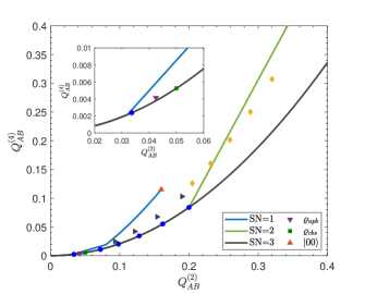
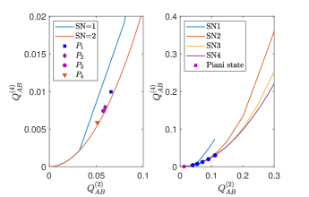
Figure 2: Entanglement dimensionality criterion based on second and fourth moments of RRMs for two-qutrit systems, formulated in Observation 2 ϱ iso subscript italic-ϱ iso \varrho_{\mathrm{iso}} p = 1 , 0.9 , 0.8 , 0.7 , 0.6 , 0.41 𝑝 1 0.9 0.8 0.7 0.6 0.41
p=1,0.9,0.8,0.7,0.6,0.41 ϱ ( v ) = v ( | 00 ⟩ + | 11 ⟩ ) ( ⟨ 00 | + ⟨ 11 | ) + ( 1 − v ) 𝟙 ⊗ 2 / 3 2 italic-ϱ 𝑣 𝑣 ket 00 ket 11 bra 00 bra 11 1 𝑣 superscript 1 tensor-product absent 2 superscript 3 2 \varrho(v)=v(|00\rangle+|11\rangle)(\langle 00|+\langle 11|)+(1-v)\mathbbm{1}^{\otimes 2}/3^{2} v = 1 , 0.9 , 0.8 , 0.7 𝑣 1 0.9 0.8 0.7
v=1,0.9,0.8,0.7 ϱ ( u ) = u ϱ 0 + ( 1 − u ) 𝟙 ⊗ 2 / 3 2 italic-ϱ 𝑢 𝑢 subscript italic-ϱ 0 1 𝑢 superscript 1 tensor-product absent 2 superscript 3 2 \varrho(u)=u\varrho_{0}+(1-u)\mathbbm{1}^{\otimes 2}/3^{2} u = 1 , 0.95 , 0.9 , 0.85 , 0.8 𝑢 1 0.95 0.9 0.85 0.8
u=1,0.95,0.9,0.85,0.8 ϱ 0 = ( 𝟙 ⊗ 2 + 2 λ 1 ⊗ λ 1 + 2 λ 3 ⊗ λ 3 ) / 3 2 subscript italic-ϱ 0 superscript 1 tensor-product absent 2 tensor-product 2 subscript 𝜆 1 subscript 𝜆 1 tensor-product 2 subscript 𝜆 3 subscript 𝜆 3 superscript 3 2 \varrho_{0}=(\mathbbm{1}^{\otimes 2}+2\lambda_{1}\otimes\lambda_{1}+2\lambda_{3}\otimes\lambda_{3})/3^{2} ϱ u p b subscript italic-ϱ 𝑢 𝑝 𝑏 \varrho_{upb} ϱ c b s subscript italic-ϱ 𝑐 𝑏 𝑠 \varrho_{cbs}
Surprisingly, Observation 2 r = 1 𝑟 1 r=1 [54 ] . Specifically, entangled states that are positive under partial transposition (PPT), that is, ϱ A B ⊤ A ≥ 0 superscript subscript italic-ϱ 𝐴 𝐵 subscript top 𝐴 0 \varrho_{AB}^{\top_{A}}\geq 0 [73 , 74 ] . In particular, as a subset of the PPT states, the partial transpose invariant (PTI) state, ϱ A B = ϱ A B ⊤ A subscript italic-ϱ 𝐴 𝐵 superscript subscript italic-ϱ 𝐴 𝐵 subscript top 𝐴 \varrho_{AB}=\varrho_{AB}^{\top_{A}} 1 ϱ c b s subscript italic-ϱ 𝑐 𝑏 𝑠 \varrho_{cbs} [75 ] and the unextendible product base state ϱ u p b subscript italic-ϱ 𝑢 𝑝 𝑏 \varrho_{upb} [55 ] . Fig. 2 [76 ] can also be detected by our criteria, see Appendix D
Detection and quantification of imaginarity.— From the resource theory of imaginarity [48 , 49 , 50 ] , the resource states are identified as imaginary states which have imaginary entries in a given basis { | j ⟩ } ket 𝑗 \{|j\rangle\} [2 , 52 ] , weak-value theory [77 ] , and quantum multiparameter metrology [78 ] .
Here, our task is to analyze and characterize imaginary states via RM frameworks. However, this is impossible if one only uses the moments R A B ( t ) superscript subscript 𝑅 𝐴 𝐵 𝑡 R_{AB}^{(t)} 1 1
Observation 3 .
Consider the second moments R A B ( 2 ) superscript subscript 𝑅 𝐴 𝐵 2 R_{AB}^{(2)} Q A B ( 2 ) superscript subscript 𝑄 𝐴 𝐵 2 Q_{AB}^{(2)} Q ^ A B ( 2 ) superscript subscript ^ 𝑄 𝐴 𝐵 2 \hat{Q}_{AB}^{(2)} ϱ A B subscript italic-ϱ 𝐴 𝐵 \varrho_{AB}
G A B ( 2 ) = ( d 2 − 1 ) 2 R A B ( 2 ) − L 2 Q A B ( 2 ) − L ^ 2 Q ^ A B ( 2 ) , superscript subscript 𝐺 𝐴 𝐵 2 superscript superscript 𝑑 2 1 2 superscript subscript 𝑅 𝐴 𝐵 2 superscript 𝐿 2 superscript subscript 𝑄 𝐴 𝐵 2 superscript ^ 𝐿 2 superscript subscript ^ 𝑄 𝐴 𝐵 2 G_{AB}^{(2)}=(d^{2}-1)^{2}R_{AB}^{(2)}-L^{2}Q_{AB}^{(2)}-\hat{L}^{2}\hat{Q}_{AB}^{(2)}, (12)
where L = ( d − 1 ) ( d + 2 ) / 2 𝐿 𝑑 1 𝑑 2 2 L=(d-1)(d+2)/2 L ^ = d ( d − 1 ) / 2 ^ 𝐿 𝑑 𝑑 1 2 \hat{L}=d(d-1)/2 Q ^ X ( 2 ) superscript subscript ^ 𝑄 𝑋 2 \hat{Q}_{X}^{(2)} ϱ X subscript italic-ϱ 𝑋 \varrho_{X} ( X = A , B ) 𝑋 𝐴 𝐵
(X=A,B)
(i) [Detection.] ϱ A B subscript italic-ϱ 𝐴 𝐵 \varrho_{AB} Q ^ A ( 2 ) = Q ^ B ( 2 ) = G A B ( 2 ) = 0 superscript subscript ^ 𝑄 𝐴 2 superscript subscript ^ 𝑄 𝐵 2 superscript subscript 𝐺 𝐴 𝐵 2 0 \hat{Q}_{A}^{(2)}=\hat{Q}_{B}^{(2)}=G_{AB}^{(2)}=0 ϱ A B subscript italic-ϱ 𝐴 𝐵 \varrho_{AB} Q ^ A ( 2 ) > 0 superscript subscript ^ 𝑄 𝐴 2 0 \hat{Q}_{A}^{(2)}>0 Q ^ B ( 2 ) > 0 superscript subscript ^ 𝑄 𝐵 2 0 \hat{Q}_{B}^{(2)}>0 G A B ( 2 ) > 0 superscript subscript 𝐺 𝐴 𝐵 2 0 G_{AB}^{(2)}>0
(ii) [Quantification.] Q ^ A ( 2 ) superscript subscript ^ 𝑄 𝐴 2 \hat{Q}_{A}^{(2)} Q ^ B ( 2 ) superscript subscript ^ 𝑄 𝐵 2 \hat{Q}_{B}^{(2)} G A B ( 2 ) superscript subscript 𝐺 𝐴 𝐵 2 G_{AB}^{(2)} ℱ R ( ϱ A B ) = min τ { μ ≥ 0 : ϱ A B + μ τ 1 + μ ∈ ℛ } subscript ℱ 𝑅 subscript italic-ϱ 𝐴 𝐵 subscript 𝜏 : 𝜇 0 subscript italic-ϱ 𝐴 𝐵 𝜇 𝜏 1 𝜇 ℛ \mathcal{F}_{R}(\varrho_{AB})=\min_{\tau}\{\mu\geq 0:\frac{\varrho_{AB}+\mu\tau}{1+\mu}\in\mathscr{R}\} [49 ] , where ℛ ℛ \mathscr{R} τ 𝜏 \tau
ℱ LB ( ϱ A B ) ≤ ℱ R ( ϱ A B ) , subscript ℱ LB subscript italic-ϱ 𝐴 𝐵 subscript ℱ 𝑅 subscript italic-ϱ 𝐴 𝐵 \mathcal{F}_{\mathrm{LB}}(\varrho_{AB})\leq\mathcal{F}_{R}(\varrho_{AB}), (13)
where
ℱ LB = 1 d L ^ ( Q ^ A ( 2 ) + Q ^ B ( 2 ) ) + G A B ( 2 ) . subscript ℱ LB 1 𝑑 ^ 𝐿 superscript subscript ^ 𝑄 𝐴 2 superscript subscript ^ 𝑄 𝐵 2 superscript subscript 𝐺 𝐴 𝐵 2 \mathcal{F}_{\mathrm{LB}}=\frac{1}{d}\sqrt{\hat{L}\left(\hat{Q}_{A}^{(2)}+\hat{Q}_{B}^{(2)}\right)+G_{AB}^{(2)}}. (14)
The proof of Observation 3 B Q ^ X ( 2 ) superscript subscript ^ 𝑄 𝑋 2 \hat{Q}_{X}^{(2)} G X = ( d 2 − 1 ) R X ( 2 ) − L Q X ( 2 ) subscript 𝐺 𝑋 superscript 𝑑 2 1 superscript subscript 𝑅 𝑋 2 𝐿 superscript subscript 𝑄 𝑋 2 G_{X}=(d^{2}-1)R_{X}^{(2)}-LQ_{X}^{(2)} 1
Table 1: Two-qutrit states: (1). ( | 00 ⟩ + i | 22 ⟩ ) / 2 ket 00 𝑖 ket 22 2 (|00\rangle+i|22\rangle)/\sqrt{2} ( | 00 ⟩ + | 11 ⟩ + i | 22 ⟩ ) / 3 ket 00 ket 11 𝑖 ket 22 3 (|00\rangle+|11\rangle+i|22\rangle)/\sqrt{3} ( i | 02 ⟩ + i | 12 ⟩ + | 10 ⟩ + | 12 ⟩ ) / 2 𝑖 ket 02 𝑖 ket 12 ket 10 ket 12 2 (i|02\rangle+i|12\rangle+|10\rangle+|12\rangle)/2 ( | 00 ⟩ + | 22 ⟩ ) / 2 ket 00 ket 22 2 (|00\rangle+|22\rangle)/\sqrt{2}
ϱ A B subscript italic-ϱ 𝐴 𝐵 \varrho_{AB} Q ^ A ( 2 ) superscript subscript ^ 𝑄 𝐴 2 \hat{Q}_{A}^{(2)} Q ^ B ( 2 ) superscript subscript ^ 𝑄 𝐵 2 \hat{Q}_{B}^{(2)} G A B ( 2 ) superscript subscript 𝐺 𝐴 𝐵 2 G_{AB}^{(2)} ℱ LB ( ϱ A B ) subscript ℱ LB subscript italic-ϱ 𝐴 𝐵 \mathcal{F}_{\mathrm{LB}}(\varrho_{AB}) ℱ R ( ϱ A B ) subscript ℱ 𝑅 subscript italic-ϱ 𝐴 𝐵 \mathcal{F}_{R}(\varrho_{AB}) Result
(1)
0 0 0 0 4.5 4.5 4.5 0.7071 0.7071 0.7071 1 1 1 Imaginary
(2)
0 0 0 0 4 4 4 0.6667 0.6667 0.6667 0.9428 0.9428 0.9428 Imaginary
(3)
0.1250 0.1250 0.1250 0.1250 0.1250 0.1250 2.6250 2.6250 2.6250 0.6124 0.6124 0.6124 0.8660 0.8660 0.8660 Imaginary
(4)
0 0 0 0 0 0 0 0 0 0 Real
Classical shadow.— The classical shadow is a powerful tool in certifying properties of quantum systems [19 , 59 , 60 ] . The standard classical shadow is based on RMs by employing random unitary and computational basis measurements.
Next, we develop the classical shadow with RRMs following (i) and (ii) in Assumptions. Applying orthogonal operation O 𝑂 O ϱ → O ϱ O ⊤ → italic-ϱ 𝑂 italic-ϱ superscript 𝑂 top \varrho\rightarrow O\varrho O^{\top} { | b ⟩ } ket 𝑏 \{|b\rangle\} O ⊤ | b ⟩ ⟨ b | O superscript 𝑂 top ket 𝑏 bra 𝑏 𝑂 O^{\top}|b\rangle\langle b|O ℳ ( ρ ) = 𝔼 [ O ⊤ | b ⟩ ⟨ b | O ] ℳ 𝜌 𝔼 delimited-[] superscript 𝑂 top ket 𝑏 bra 𝑏 𝑂 \mathcal{M}(\rho)=\mathbb{E}\left[O^{\top}|b\rangle\langle b|O\right] ϱ ~ = 𝔼 [ ℳ − 1 ( O ⊤ | b ⟩ ⟨ b | O ) ] ~ italic-ϱ 𝔼 delimited-[] superscript ℳ 1 superscript 𝑂 top ket 𝑏 bra 𝑏 𝑂 \tilde{\varrho}=\mathbb{E}\left[\mathcal{M}^{-1}\left(O^{\top}|b\rangle\langle b|O\right)\right] ℳ − 1 superscript ℳ 1 \mathcal{M}^{-1} ℳ ( ϱ ) ℳ italic-ϱ \mathcal{M}(\varrho)
Observation 4 .
By performing a global orthogonal matrix O 𝑂 O N 𝑁 N ϱ italic-ϱ \varrho
ℳ ( ϱ ) = 𝟙 d N + 2 ϱ d N + 2 , ℳ − 1 ( ϱ ) = d N + 2 2 ϱ − 1 2 𝟙 d N . formulae-sequence ℳ italic-ϱ subscript 1 superscript 𝑑 𝑁 2 italic-ϱ superscript 𝑑 𝑁 2 superscript ℳ 1 italic-ϱ superscript 𝑑 𝑁 2 2 italic-ϱ 1 2 subscript 1 superscript 𝑑 𝑁 \mathcal{M}(\varrho)=\frac{\mathbbm{1}_{d^{N}}+2\varrho}{d^{N}+2},\quad\mathcal{M}^{-1}(\varrho)=\frac{d^{N}+2}{2}\varrho-\frac{1}{2}\mathbbm{1}_{d^{N}}. (15)
The proof of Observation 4 B 7 N O subscript 𝑁 𝑂 N_{O} K 𝐾 K { ϱ ~ ( m ) } m = 1 N O superscript subscript superscript ~ italic-ϱ 𝑚 𝑚 1 subscript 𝑁 𝑂 \{\tilde{\varrho}^{(m)}\}_{m=1}^{N_{O}} ϱ italic-ϱ \varrho
To test Observation 4 N 𝑁 N ϱ p = ( 1 − p ) | GHZ + ⟩ ⟨ GHZ + | + p | GHZ − ⟩ ⟨ GHZ − | subscript italic-ϱ 𝑝 1 𝑝 ket subscript GHZ quantum-operator-product subscript GHZ 𝑝 subscript GHZ bra subscript GHZ \varrho_{p}=(1-p)|{\mathrm{GHZ}}_{+}\rangle\langle{\mathrm{GHZ}}_{+}|+p|{\mathrm{GHZ}}_{-}\rangle\langle{\mathrm{GHZ}}_{-}| p ∈ [ 0 , 1 ] 𝑝 0 1 p\in[0,1] | GHZ ± ⟩ = ( | 0 ⟩ ⊗ N ± | 1 ⟩ ⊗ N ) / 2 ket subscript GHZ plus-or-minus plus-or-minus superscript ket 0 tensor-product absent 𝑁 superscript ket 1 tensor-product absent 𝑁 2 |{\mathrm{GHZ}}_{\pm}\rangle=(|0\rangle^{\otimes N}\pm|1\rangle^{\otimes N})/\sqrt{2} f es = tr ( ϱ ~ p | GHZ + ⟩ ⟨ GHZ + | ) subscript 𝑓 es tr subscript ~ italic-ϱ 𝑝 ket subscript GHZ bra subscript GHZ f_{\mathrm{es}}={\mathrm{tr}}(\tilde{\varrho}_{p}|{\mathrm{GHZ}}_{+}\rangle\langle{\mathrm{GHZ}}_{+}|) ϱ ~ p subscript ~ italic-ϱ 𝑝 \tilde{\varrho}_{p} ϱ p subscript italic-ϱ 𝑝 \varrho_{p} f es subscript 𝑓 es f_{\mathrm{es}} f ex = tr ( ϱ p | GHZ + ⟩ ⟨ GHZ + | ) = 1 − p subscript 𝑓 ex tr subscript italic-ϱ 𝑝 ket subscript GHZ bra subscript GHZ 1 𝑝 f_{\mathrm{ex}}={\mathrm{tr}}({\varrho}_{p}|{\mathrm{GHZ}}_{+}\rangle\langle{\mathrm{GHZ}}_{+}|)=1-p 3 | f es − f ex | subscript 𝑓 es subscript 𝑓 ex |f_{\mathrm{es}}-f_{\mathrm{ex}}| 5 5 5 ϱ p subscript italic-ϱ 𝑝 \varrho_{p}
We remark that standard classical shadows can also be implemented via local unitary matrices to predict the properties of any state [19 ] , but not for local orthogonal matrices. In Appendix E E [16 ] .
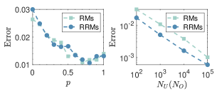
Figure 3: (a) The average of the error | f es − f ex | subscript 𝑓 es subscript 𝑓 ex |f_{\mathrm{es}}-f_{\mathrm{ex}}| p 𝑝 p N U = N O = 100 subscript 𝑁 𝑈 subscript 𝑁 𝑂 100 N_{U}=N_{O}=100 K = 10 3 𝐾 superscript 10 3 K=10^{3} 4 | X A B ( 2 ) − X ~ A B ( 2 ) | superscript subscript 𝑋 𝐴 𝐵 2 superscript subscript ~ 𝑋 𝐴 𝐵 2 |X_{AB}^{(2)}-\tilde{X}_{AB}^{(2)}| ( | 00 ⟩ + | 11 ⟩ ) / 2 ket 00 ket 11 2 (|00\rangle+|11\rangle)/\sqrt{2} X A B ( 2 ) , X ~ A B ( 2 ) superscript subscript 𝑋 𝐴 𝐵 2 superscript subscript ~ 𝑋 𝐴 𝐵 2
X_{AB}^{(2)},\tilde{X}_{AB}^{(2)} X = R , Q 𝑋 𝑅 𝑄
X=R,Q X ~ A B ( 2 ) = N V − 1 ∑ j = 1 N V tr ( V j ϱ V j † M A ⊗ M B ) 2 superscript subscript ~ 𝑋 𝐴 𝐵 2 superscript subscript 𝑁 𝑉 1 superscript subscript 𝑗 1 subscript 𝑁 𝑉 tr superscript tensor-product subscript 𝑉 𝑗 italic-ϱ superscript subscript 𝑉 𝑗 † subscript 𝑀 𝐴 subscript 𝑀 𝐵 2 \tilde{X}_{AB}^{(2)}=N_{V}^{-1}\sum_{j=1}^{N_{V}}{\mathrm{tr}}(V_{j}\varrho V_{j}^{{\dagger}}M_{A}\otimes M_{B})^{2} V j = V A ( j ) ⊗ V B ( j ) subscript 𝑉 𝑗 tensor-product superscript subscript 𝑉 𝐴 𝑗 superscript subscript 𝑉 𝐵 𝑗 V_{j}=V_{A}^{(j)}\otimes V_{B}^{(j)} V = U , O 𝑉 𝑈 𝑂
V=U,O
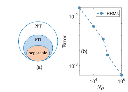
Experimental considerations.— Our protocols have advantages related to the experimental settings compared to standard RMs. One is that fewer experimental steps are required for performing an orthogonal matrix. In photonic systems, 1 / 2 1 2 1/2 [50 ] . Another is that fewer random operations are enough for certain tasks. In Fig. 3 10 3 superscript 10 3 10^{3} 4.6 × 10 − 3 4.6 superscript 10 3 4.6\times 10^{-3} 10 5 superscript 10 5 10^{5}
An important step in implementing our protocols is to generate Haar random orthogonal matrices following the known algorithms [79 , 80 ] . To check whether the sample matrices are indeed Haar random, one can apply the frame potential [81 , 82 , 83 ] for orthogonal matrices [47 ] .
Conclusion.— In this work, we have introduced the concepts of RRMs and PRRMs to characterize quantum states. We have shown that RRMs can detect bound entanglement and dimensionality, while the combination of RMs, RRMs, and PRRMs can characterize imaginary states. We have also extended the classical shadow by using random orthogonal matrices. Our results provide simplified experimental strategies to analyze high-dimensional quantum states using more easily performed orthogonal operations.
Several potential avenues for further investigation arise from our research. First, while we considered the orthogonal versions of RMs, developing RMs within different subsets of unitaries would be interesting. This could motivate further investigations of quantum resources beyond entanglement and imaginarity. Second, it would be worthwhile to find stronger entanglement criteria than the criterion by RMs itself, e.g., using linear or nonlinear combination in the space of Q A B subscript 𝑄 𝐴 𝐵 Q_{AB} Q ^ A B subscript ^ 𝑄 𝐴 𝐵 \hat{Q}_{AB} [40 ] . Finally, it would be desirable to verify our results in different experimental platforms such as trapped ions [22 ] , Rydberg atoms [15 ] , and photonic systems [40 , 84 ] .
Acknowledgment.— We thank Feng-Xiao Sun, Jiajie Guo, Nikolai Wyderka, Xiao-Dong Yu, Yu Xiang, and Zhenhuan Liu for useful discussions. This work is supported by the National Natural Science Foundation of China (Grant Nos. 12125402, 12347152, 12405005, 12405006, 12075159, and 12171044), Beijing Natural Science Foundation (Grant No. Z240007), and the Innovation Program for Quantum Science and Technology (No. 2021ZD0301500), the Postdoctoral Fellowship Program of CPSF (No. GZC20230103), the China Postdoctoral Science Foundation (No. 2023M740118 and 2023M740119), the specific research fund of the Innovation Platform for Academicians of Hainan Province, the Deutsche Forschungsgemeinschaft (DFG, German Research Foundation, project numbers 447948357 and 440958198), the Sino-German Center for Research Promotion (Project M-0294), and the German Ministry of Education and Research (Project QuKuK, BMBF Grant No. 16KIS1618K). Satoya Imai acknowledges the European Commission through the H2020 QuantERA ERA-NET Cofund in Quantum Technologies projects "MENTA".
Note added: After finishing our work, similar ideas on classical shdows with RRMs have also been discussed in [85 ] .
Contents
A Preliminaries and calculation of second-order moments
A.1 Moments over orthogonal groupA.2 Useful properties of the generalized Gell-Mann matrices
A.3 Moments of RRMs and PRRMs
A.3.1 Single-qudit systemsA.3.2 Two-qudit systemA.3.3 Multipartite systems
B Proofs of the observations in the main textC Estimating the moments of bipartite systems from random rotationsD Other numerical results and analytic lower bound
E Generalized results
E.1 Entanglement criterion of N 𝑁 N E.2 Imaginarity detection criterion and quantification of multi-qudit statesE.3 Classical shadow with RRMs
E.4 Cross-platform verification of quantum devices
E.4.1 Estimation of the overlap between bipartite states from local orthogonal matricesE.4.2 Estimation of the overlap between multipartite states from global and local orthogonal matrices
The following appendices A E A B C D E
Appendix A Preliminaries and calculation of second-order moments
A.1 Moments over orthogonal group
Let us start by introducing the notation used in this work. We denote the set of linear operators that act on the d 𝑑 d ℂ d superscript ℂ 𝑑 \mathds{C}^{d} ℒ ( ℂ d ) ℒ superscript ℂ 𝑑 \mathcal{L}(\mathds{C}^{d}) d 𝑑 d 𝟙 d subscript 1 𝑑 \mathbbm{1}_{d} 𝐎 ( d ) 𝐎 𝑑 \bm{\mathrm{O}}(d) O ∈ ℒ ( ℂ d ) 𝑂 ℒ superscript ℂ 𝑑 O\in\mathcal{L}(\mathds{C}^{d}) O O ⊤ = O ⊤ O = 𝟙 d 𝑂 superscript 𝑂 top superscript 𝑂 top 𝑂 subscript 1 𝑑 OO^{\top}=O^{\top}O=\mathbbm{1}_{d} 𝐎 ( d ) 𝐎 𝑑 \bm{\mathrm{O}}(d) μ 𝜇 \mu Haar measure , and we will denote integrals to the Haar measure as ∫ 𝑑 O differential-d 𝑂 \int dO
By introducing two important operators, the SWAP operator, 𝕊 = ∑ j , k = 0 d − 1 | j k ⟩ ⟨ k j | 𝕊 superscript subscript 𝑗 𝑘
0 𝑑 1 ket 𝑗 𝑘 bra 𝑘 𝑗 \mathbb{S}=\sum_{j,k=0}^{d-1}|jk\rangle\langle kj| Π = ∑ j , k = 0 d − 1 | j j ⟩ ⟨ k k | Π superscript subscript 𝑗 𝑘
0 𝑑 1 ket 𝑗 𝑗 bra 𝑘 𝑘 \Pi=\sum_{j,k=0}^{d-1}|jj\rangle\langle kk|
Lemma 1 .
(First and second moment). Given 𝒜 1 ∈ ℒ ( ℂ d ) subscript 𝒜 1 ℒ superscript ℂ 𝑑 \mathcal{A}_{1}\in\mathcal{L}(\mathds{C}^{d}) 𝒜 2 ∈ ℒ ( ℂ d ⊗ ℂ d ) subscript 𝒜 2 ℒ tensor-product superscript ℂ 𝑑 superscript ℂ 𝑑 \mathcal{A}_{2}\in\mathcal{L}(\mathds{C}^{d}\otimes\mathds{C}^{d})
∫ 𝑑 O O 𝒜 1 O ⊤ differential-d 𝑂 𝑂 subscript 𝒜 1 superscript 𝑂 top \displaystyle\int dOO\mathcal{A}_{1}O^{\top} = tr ( 𝒜 1 ) d 𝟙 d , absent tr subscript 𝒜 1 𝑑 subscript 1 𝑑 \displaystyle=\frac{{\mathrm{tr}}(\mathcal{A}_{1})}{d}\mathbbm{1}_{d}, (16)
∫ 𝑑 O O ⊗ 2 𝒜 2 O ⊤ ⊗ 2 differential-d 𝑂 superscript 𝑂 tensor-product absent 2 subscript 𝒜 2 superscript 𝑂 top tensor-product absent 2
\displaystyle\int dO\,O^{\otimes 2}\mathcal{A}_{2}O^{\top\otimes 2} = γ 1 𝟙 d ⊗ 𝟙 d + γ 2 𝕊 + γ 3 Π , absent tensor-product subscript 𝛾 1 subscript 1 𝑑 subscript 1 𝑑 subscript 𝛾 2 𝕊 subscript 𝛾 3 Π \displaystyle=\gamma_{1}\mathbbm{1}_{d}\otimes\mathbbm{1}_{d}+\gamma_{2}\mathbb{S}+\gamma_{3}\Pi, (17)
where coefficients are
γ 1 subscript 𝛾 1 \displaystyle\gamma_{1} = ( d + 1 ) tr ( 𝒜 2 ) − tr ( 𝕊 𝒜 2 ) − tr ( Π 𝒜 2 ) d ( d − 1 ) ( d + 2 ) , absent 𝑑 1 tr subscript 𝒜 2 tr 𝕊 subscript 𝒜 2 tr Π subscript 𝒜 2 𝑑 𝑑 1 𝑑 2 \displaystyle=\frac{(d+1){\mathrm{tr}}(\mathcal{A}_{2})-{\mathrm{tr}}(\mathbb{S}\mathcal{A}_{2})-{\mathrm{tr}}(\Pi\mathcal{A}_{2})}{d(d-1)(d+2)}, (18)
γ 2 subscript 𝛾 2 \displaystyle\gamma_{2} = − tr ( 𝒜 2 ) + ( d + 1 ) tr ( 𝕊 𝒜 2 ) − tr ( Π 𝒜 2 ) d ( d − 1 ) ( d + 2 ) , absent tr subscript 𝒜 2 𝑑 1 tr 𝕊 subscript 𝒜 2 tr Π subscript 𝒜 2 𝑑 𝑑 1 𝑑 2 \displaystyle=\frac{-{\mathrm{tr}}(\mathcal{A}_{2})+(d+1){\mathrm{tr}}(\mathbb{S}\mathcal{A}_{2})-{\mathrm{tr}}(\Pi\mathcal{A}_{2})}{d(d-1)(d+2)}, (19)
γ 3 subscript 𝛾 3 \displaystyle\gamma_{3} = − tr ( 𝒜 2 ) − tr ( 𝕊 𝒜 2 ) + ( d + 1 ) tr ( Π 𝒜 2 ) d ( d − 1 ) ( d + 2 ) . absent tr subscript 𝒜 2 tr 𝕊 subscript 𝒜 2 𝑑 1 tr Π subscript 𝒜 2 𝑑 𝑑 1 𝑑 2 \displaystyle=\frac{-{\mathrm{tr}}(\mathcal{A}_{2})-{\mathrm{tr}}(\mathbb{S}\mathcal{A}_{2})+(d+1){\mathrm{tr}}(\Pi\mathcal{A}_{2})}{d(d-1)(d+2)}. (20)
Proof.
The first-order moment is proportional to the identity operator, i.e. ∫ 𝑑 O O 𝒜 1 O ⊤ = α 𝟙 d differential-d 𝑂 𝑂 subscript 𝒜 1 superscript 𝑂 top 𝛼 subscript 1 𝑑 \int dOO\mathcal{A}_{1}O^{\top}=\alpha\mathbbm{1}_{d} α ∈ ℂ 𝛼 ℂ \alpha\in\mathds{C} α = tr ( 𝒜 1 ) d 𝛼 tr subscript 𝒜 1 𝑑 \alpha=\frac{{\mathrm{tr}}(\mathcal{A}_{1})}{d}
The second moment is a linear combination of three operators 𝟙 d ⊗ 𝟙 d tensor-product subscript 1 𝑑 subscript 1 𝑑 \mathbbm{1}_{d}\otimes\mathbbm{1}_{d} 𝕊 𝕊 \mathbb{S} Π Π \Pi [66 ] ,
∫ 𝑑 O ( O ⊗ O ) 𝒜 2 ( O ⊤ ⊗ O ⊤ ) = γ 1 𝟙 d ⊗ 𝟙 d + γ 2 𝕊 + γ 3 Π . differential-d 𝑂 tensor-product 𝑂 𝑂 subscript 𝒜 2 tensor-product superscript 𝑂 top superscript 𝑂 top tensor-product subscript 𝛾 1 subscript 1 𝑑 subscript 1 𝑑 subscript 𝛾 2 𝕊 subscript 𝛾 3 Π \displaystyle\int dO(O\otimes O)\mathcal{A}_{2}(O^{\top}\otimes O^{\top})=\gamma_{1}\mathbbm{1}_{d}\otimes\mathbbm{1}_{d}+\gamma_{2}\mathbb{S}+\gamma_{3}\Pi. (21)
To find the coefficients, we left-multiply both sides by 𝟙 d ⊗ 𝟙 d tensor-product subscript 1 𝑑 subscript 1 𝑑 \mathbbm{1}_{d}\otimes\mathbbm{1}_{d} 𝕊 𝕊 \mathbb{S} Π Π \Pi
( tr ( 𝒜 2 ) tr ( 𝕊 𝒜 2 ) tr ( Π 𝒜 2 ) ) = d ( d 1 1 1 d 1 1 1 d ) ( γ 1 γ 2 γ 3 ) matrix tr subscript 𝒜 2 tr 𝕊 subscript 𝒜 2 tr Π subscript 𝒜 2 𝑑 matrix 𝑑 1 1 1 𝑑 1 1 1 𝑑 matrix subscript 𝛾 1 subscript 𝛾 2 subscript 𝛾 3 \displaystyle\begin{pmatrix}{\mathrm{tr}}(\mathcal{A}_{2})\\
{\mathrm{tr}}(\mathbb{S}\mathcal{A}_{2})\\
{\mathrm{tr}}(\Pi\mathcal{A}_{2})\end{pmatrix}=d\begin{pmatrix}d&1&1\\
1&d&1\\
1&1&d\end{pmatrix}\begin{pmatrix}\gamma_{1}\\
\gamma_{2}\\
\gamma_{3}\end{pmatrix} (22)
During the calculation, we use the fact that tr ( 𝟙 d ⊗ 𝟙 d ) = d 2 tr tensor-product subscript 1 𝑑 subscript 1 𝑑 superscript 𝑑 2 {\mathrm{tr}}(\mathbbm{1}_{d}\otimes\mathbbm{1}_{d})=d^{2} tr ( 𝕊 ) = tr ( Π ) = d tr 𝕊 tr Π 𝑑 {\mathrm{tr}}(\mathbb{S})={\mathrm{tr}}(\Pi)=d
In general, the t 𝑡 t ( 2 t ) ! 2 t t ! 2 𝑡 superscript 2 𝑡 𝑡 \frac{(2t)!}{2^{t}t!} [86 ] and the Schur-Weyl duality for orthogonal groups [67 ] . For instance, the fourth moment can be represented as a linear combination of 105 105 105
Lemma 2 .
For any two operators 𝒜 , ℬ ∈ ℒ ( ℂ d ) 𝒜 ℬ
ℒ superscript ℂ 𝑑 \mathcal{A},\mathcal{B}\in\mathcal{L}(\mathds{C}^{d}) tr ( Π 𝒜 ⊗ ℬ ) = tr ( 𝕊 𝒜 ⊗ ℬ ⊤ ) tr tensor-product Π 𝒜 ℬ tr tensor-product 𝕊 𝒜 superscript ℬ top {\mathrm{tr}}(\Pi\mathcal{A}\otimes\mathcal{B})={\mathrm{tr}}(\mathbb{S}\mathcal{A}\otimes\mathcal{B}^{\top})
Proof.
Note that the operator Π Π \Pi
Π = ∑ j , k = 0 d − 1 | j j ⟩ ⟨ k k | = ∑ j , k = 0 d − 1 | j ⟩ ⟨ k | ⊗ | j ⟩ ⟨ k | = ∑ j , k = 0 d − 1 | j ⟩ ⟨ k | ⊗ ( | j ⟩ ⟨ k | ) ⊤ = 𝕊 ⊤ 2 , Π superscript subscript 𝑗 𝑘
0 𝑑 1 ket 𝑗 𝑗 bra 𝑘 𝑘 superscript subscript 𝑗 𝑘
0 𝑑 1 tensor-product ket 𝑗 bra 𝑘 ket 𝑗 bra 𝑘 superscript subscript 𝑗 𝑘
0 𝑑 1 tensor-product ket 𝑗 bra 𝑘 superscript ket 𝑗 bra 𝑘 top superscript 𝕊 subscript top 2 \displaystyle\Pi=\sum_{j,k=0}^{d-1}|jj\rangle\langle kk|=\sum_{j,k=0}^{d-1}|j\rangle\langle k|\otimes|j\rangle\langle k|=\sum_{j,k=0}^{d-1}|j\rangle\langle k|\otimes(|j\rangle\langle k|)^{\top}=\mathbb{S}^{\top_{2}}, (23)
where A ⊤ superscript 𝐴 top A^{\top} A 𝐴 A ⊤ 2 subscript top 2 \top_{2}
tr ( Π 𝒜 ⊗ ℬ ) tr tensor-product Π 𝒜 ℬ \displaystyle{\mathrm{tr}}(\Pi\mathcal{A}\otimes\mathcal{B}) = tr ( 𝕊 ⊤ 2 𝒜 ⊗ ℬ ) = tr ( 𝕊 𝒜 ⊗ ℬ ⊤ ) . absent tr tensor-product superscript 𝕊 subscript top 2 𝒜 ℬ tr tensor-product 𝕊 𝒜 superscript ℬ top \displaystyle={\mathrm{tr}}(\mathbb{S}^{\top_{2}}\mathcal{A}\otimes\mathcal{B})={\mathrm{tr}}(\mathbb{S}\mathcal{A}\otimes\mathcal{B}^{\top}). (24)
∎
A.2 Useful properties of the generalized Gell-Mann matrices
The generalized Gell-Mann matrices (GGMs) are extensions of the Gell-Mann matrices, which are originally defined for qutrit systems. The GGMs are denoted as { λ j } j = 1 d 2 − 1 superscript subscript subscript 𝜆 𝑗 𝑗 1 superscript 𝑑 2 1 \{\lambda_{j}\}_{j=1}^{d^{2}-1} λ 0 = 𝟙 d subscript 𝜆 0 subscript 1 𝑑 \lambda_{0}=\mathbbm{1}_{d} λ j subscript 𝜆 𝑗 \lambda_{j} λ j = λ j † subscript 𝜆 𝑗 superscript subscript 𝜆 𝑗 † \lambda_{j}=\lambda_{j}^{{\dagger}} tr ( λ j λ k ) = d δ j k tr subscript 𝜆 𝑗 subscript 𝜆 𝑘 𝑑 subscript 𝛿 𝑗 𝑘 {\mathrm{tr}}(\lambda_{j}\lambda_{k})=d\delta_{jk} tr ( λ j ) = 0 tr subscript 𝜆 𝑗 0 {\mathrm{tr}}(\lambda_{j})=0 j > 0 𝑗 0 j>0 [87 ] . The GGMs consist of three different types of matrices [64 ] ,
(i) d ( d − 1 ) 2 𝑑 𝑑 1 2 \frac{d(d-1)}{2}
λ j k ( s ) = d 2 ( | j ⟩ ⟨ k | + | k ⟩ ⟨ j | ) , 0 ≤ j < k ≤ d − 1 . formulae-sequence superscript subscript 𝜆 𝑗 𝑘 𝑠 𝑑 2 ket 𝑗 bra 𝑘 ket 𝑘 bra 𝑗 0 𝑗 𝑘 𝑑 1 \displaystyle\lambda_{jk}^{(s)}=\sqrt{\frac{d}{2}}\left(|j\rangle\langle k|+|k\rangle\langle j|\right),\quad 0\leq j<k\leq d-1. (25)
(ii) d ( d − 1 ) 2 𝑑 𝑑 1 2 \frac{d(d-1)}{2}
λ j k ( a ) = d 2 ( − i | j ⟩ ⟨ k | + i | k ⟩ ⟨ j | ) , 0 ≤ j < k ≤ d − 1 . formulae-sequence superscript subscript 𝜆 𝑗 𝑘 𝑎 𝑑 2 𝑖 ket 𝑗 quantum-operator-product 𝑘 𝑖 𝑘 bra 𝑗 0 𝑗 𝑘 𝑑 1 \displaystyle\lambda_{jk}^{(a)}=\sqrt{\frac{d}{2}}\left(-i|j\rangle\langle k|+i|k\rangle\langle j|\right),\quad 0\leq j<k\leq d-1. (26)
(iii) d − 1 𝑑 1 d-1
λ l ( d ) = d ( l + 1 ) ( l + 2 ) [ − ( l + 1 ) | l + 1 ⟩ ⟨ l + 1 | + ∑ j = 0 l | j ⟩ ⟨ j | ] , 0 ≤ l ≤ d − 2 . formulae-sequence superscript subscript 𝜆 𝑙 𝑑 𝑑 𝑙 1 𝑙 2 delimited-[] 𝑙 1 ket 𝑙 1 quantum-operator-product 𝑙 1 superscript subscript 𝑗 0 𝑙 𝑗 bra 𝑗 0 𝑙 𝑑 2 \displaystyle\lambda_{l}^{(d)}=\sqrt{\frac{d}{(l+1)(l+2)}}\left[-(l+1)|l+1\rangle\langle l+1|+\sum_{j=0}^{l}|j\rangle\langle j|\right],\quad 0\leq l\leq d-2. (27)
It is important to note that all symmetric and diagonal Gell-Mann matrices have real elements and satisfy Assumptions (ii) in the main text. On the other hand, all antisymmetric Gell-Mann matrices have imaginary elements and satisfy Assumptions (iii) in the main text. As a result, we can divide the Gell-Mann matrices into two categories: real Gell-Mann matrices denoted as 𝝀 = { λ 1 Re , ⋯ , λ L Re } 𝝀 superscript subscript 𝜆 1 Re ⋯ superscript subscript 𝜆 𝐿 Re \bm{\lambda}=\{\lambda_{1}^{\mathrm{Re}},\cdots,\lambda_{L}^{\mathrm{Re}}\} 𝝀 ^ = { λ 1 Im , ⋯ , λ L ^ Im } ^ 𝝀 superscript subscript 𝜆 1 Im ⋯ superscript subscript 𝜆 ^ 𝐿 Im \hat{\bm{\lambda}}=\{\lambda_{1}^{\mathrm{Im}},\cdots,\lambda_{\hat{L}}^{\mathrm{Im}}\} L = ( d − 1 ) ( d + 2 ) 2 𝐿 𝑑 1 𝑑 2 2 L=\frac{(d-1)(d+2)}{2} L ^ = d ( d − 1 ) 2 ^ 𝐿 𝑑 𝑑 1 2 \hat{L}=\frac{d(d-1)}{2} L + L ^ = d 2 − 1 𝐿 ^ 𝐿 superscript 𝑑 2 1 L+\hat{L}=d^{2}-1
Lemma 3 .
For two GGMs 𝒜 𝒜 \mathcal{A} ℬ ℬ \mathcal{B} ℋ ∈ ℂ d × d ℋ superscript ℂ 𝑑 𝑑 \mathcal{H}\in\mathbb{C}^{d\times d}
tr ( Π 𝒜 ⊗ ℬ ) = { d , 𝒜 = ℬ ∈ 𝝀 − d , 𝒜 = ℬ ∈ 𝝀 ^ 0 , o t h e r w i s e . . tr tensor-product Π 𝒜 ℬ cases 𝑑 𝒜 ℬ 𝝀 𝑑 𝒜 ℬ ^ 𝝀 0 𝑜 𝑡 ℎ 𝑒 𝑟 𝑤 𝑖 𝑠 𝑒 \displaystyle{\mathrm{tr}}(\Pi\mathcal{A}\otimes\mathcal{B})=\begin{cases}d,&\mathcal{A}=\mathcal{B}\in\bm{\lambda}\\
-d,&\mathcal{A}=\mathcal{B}\in\hat{\bm{\lambda}}\\
0,&otherwise.\\
\end{cases}. (28)
Proof.
Based on Lemma 2
tr ( Π 𝒜 ⊗ ℬ ) = tr ( 𝕊 𝒜 ⊗ ℬ ⊤ ) = { tr ( 𝒜 ℬ ) , ℬ ∈ 𝝀 − tr ( 𝒜 ℬ ) , ℬ ∈ 𝝀 ^ . tr tensor-product Π 𝒜 ℬ tr tensor-product 𝕊 𝒜 superscript ℬ top cases tr 𝒜 ℬ ℬ 𝝀 tr 𝒜 ℬ ℬ ^ 𝝀 \displaystyle{\mathrm{tr}}(\Pi\mathcal{A}\otimes\mathcal{B})={\mathrm{tr}}(\mathbb{S}\mathcal{A}\otimes\mathcal{B}^{\top})=\begin{cases}{\mathrm{tr}}(\mathcal{A}\mathcal{B}),&\mathcal{B}\in\bm{\lambda}\\
-{\mathrm{tr}}(\mathcal{A}\mathcal{B}),&\mathcal{B}\in\hat{\bm{\lambda}}\\
\end{cases}. (29)
The proof is completed by using tr ( λ j λ k ) = d δ j k tr subscript 𝜆 𝑗 subscript 𝜆 𝑘 𝑑 subscript 𝛿 𝑗 𝑘 {\mathrm{tr}}(\lambda_{j}\lambda_{k})=d\delta_{jk} λ j subscript 𝜆 𝑗 \lambda_{j} λ k subscript 𝜆 𝑘 \lambda_{k}
A.3 Moments of RRMs and PRRMs
In this subsection, we derive the second moment for quantum states of single-qudit, two-qudit, and N 𝑁 N
A.3.1 Single-qudit systems
Consider a single qudit state ϱ = 1 d ∑ j = 0 d 2 − 1 T j λ j italic-ϱ 1 𝑑 superscript subscript 𝑗 0 superscript 𝑑 2 1 subscript 𝑇 𝑗 subscript 𝜆 𝑗 \varrho=\frac{1}{d}\sum_{j=0}^{d^{2}-1}T_{j}\lambda_{j} M 𝑀 M tr ( M ) = 0 tr 𝑀 0 {\mathrm{tr}}(M)=0 tr ( M 2 ) = d tr superscript 𝑀 2 𝑑 {\mathrm{tr}}(M^{2})=d
Q ( 2 ) superscript 𝑄 2 \displaystyle Q^{(2)} = ∫ 𝑑 O [ tr ( O ϱ O ⊤ M ) ] 2 = 1 d 2 ∑ j , k = 0 d 2 − 1 T j T k tr ( Φ ) , absent differential-d 𝑂 superscript delimited-[] tr 𝑂 italic-ϱ superscript 𝑂 top 𝑀 2 1 superscript 𝑑 2 superscript subscript 𝑗 𝑘
0 superscript 𝑑 2 1 subscript 𝑇 𝑗 subscript 𝑇 𝑘 tr Φ \displaystyle=\int dO\left[{\mathrm{tr}}\left(O\varrho O^{\top}M\right)\right]^{2}=\frac{1}{d^{2}}\sum_{j,k=0}^{d^{2}-1}T_{j}T_{k}{\mathrm{tr}}(\Phi), (30)
where the quantity
tr ( Φ ) tr Φ \displaystyle{\mathrm{tr}}(\Phi) = tr [ ∫ 𝑑 O ( O ⊗ O ) ( λ j ⊗ λ k ) ( O ⊤ ⊗ O ⊤ ) ( M ⊗ M ) ] absent tr delimited-[] differential-d 𝑂 tensor-product 𝑂 𝑂 tensor-product subscript 𝜆 𝑗 subscript 𝜆 𝑘 tensor-product superscript 𝑂 top superscript 𝑂 top tensor-product 𝑀 𝑀 \displaystyle={\mathrm{tr}}\left[\int dO\left(O\otimes O\right)(\lambda_{j}\otimes\lambda_{k})\left(O^{\top}\otimes O^{\top}\right)\left(M\otimes M\right)\right] (31)
= γ 2 tr ( 𝕊 M ⊗ M ) + γ 3 tr ( Π M ⊗ M ) absent subscript 𝛾 2 tr tensor-product 𝕊 𝑀 𝑀 subscript 𝛾 3 tr tensor-product Π 𝑀 𝑀 \displaystyle=\gamma_{2}{\mathrm{tr}}(\mathbb{S}M\otimes M)+\gamma_{3}{\mathrm{tr}}(\Pi M\otimes M) (32)
= d ( γ 2 + γ 3 ) absent 𝑑 subscript 𝛾 2 subscript 𝛾 3 \displaystyle=d\left(\gamma_{2}+\gamma_{3}\right) (33)
The third equation uses the fact that tr ( 𝕊 M ⊗ M ) = tr ( Π M ⊗ M ) = tr ( M 2 ) = d tr tensor-product 𝕊 𝑀 𝑀 tr tensor-product Π 𝑀 𝑀 tr superscript 𝑀 2 𝑑 {\mathrm{tr}}(\mathbb{S}M\otimes M)={\mathrm{tr}}(\Pi M\otimes M)={\mathrm{tr}}(M^{2})=d
γ 2 subscript 𝛾 2 \displaystyle\gamma_{2} = ( d + 1 ) d ( d − 1 ) ( d + 2 ) d δ j k − 1 d ( d − 1 ) ( d + 2 ) tr ( Π λ j ⊗ λ k ) , absent 𝑑 1 𝑑 𝑑 1 𝑑 2 𝑑 subscript 𝛿 𝑗 𝑘 1 𝑑 𝑑 1 𝑑 2 tr tensor-product Π subscript 𝜆 𝑗 subscript 𝜆 𝑘 \displaystyle=\frac{(d+1)}{d(d-1)(d+2)}d\delta_{jk}-\frac{1}{d(d-1)(d+2)}{\mathrm{tr}}(\Pi\lambda_{j}\otimes\lambda_{k}), (34)
γ 3 subscript 𝛾 3 \displaystyle\gamma_{3} = − 1 d ( d − 1 ) ( d + 2 ) d δ j k + ( d + 1 ) d ( d − 1 ) ( d + 2 ) tr ( Π λ j ⊗ λ k ) . absent 1 𝑑 𝑑 1 𝑑 2 𝑑 subscript 𝛿 𝑗 𝑘 𝑑 1 𝑑 𝑑 1 𝑑 2 tr tensor-product Π subscript 𝜆 𝑗 subscript 𝜆 𝑘 \displaystyle=-\frac{1}{d(d-1)(d+2)}d\delta_{jk}+\frac{(d+1)}{d(d-1)(d+2)}{\mathrm{tr}}(\Pi\lambda_{j}\otimes\lambda_{k}). (35)
Following the Lemma 1
tr ( Φ ) tr Φ \displaystyle{\mathrm{tr}}(\Phi) = d ( γ 2 + γ 3 ) = d 2 δ j k + d tr ( Π λ j ⊗ λ k ) ( d − 1 ) ( d + 2 ) = { 2 d 2 δ j k ( d − 1 ) ( d + 2 ) , λ k ∈ 𝝀 0 , λ k ∈ 𝝀 ^ . absent 𝑑 subscript 𝛾 2 subscript 𝛾 3 superscript 𝑑 2 subscript 𝛿 𝑗 𝑘 𝑑 tr tensor-product Π subscript 𝜆 𝑗 subscript 𝜆 𝑘 𝑑 1 𝑑 2 cases 2 superscript 𝑑 2 subscript 𝛿 𝑗 𝑘 𝑑 1 𝑑 2 subscript 𝜆 𝑘 𝝀 0 subscript 𝜆 𝑘 ^ 𝝀 \displaystyle=d\left(\gamma_{2}+\gamma_{3}\right)=\frac{d^{2}\delta_{jk}+d{\mathrm{tr}}(\Pi\lambda_{j}\otimes\lambda_{k})}{(d-1)(d+2)}=\begin{cases}\frac{2d^{2}\delta_{jk}}{(d-1)(d+2)},&\lambda_{k}\in\bm{\lambda}\\
0,&\lambda_{k}\in\hat{\bm{\lambda}}\\
\end{cases}. (36)
Using Lemma 3
Q ( 2 ) superscript 𝑄 2 \displaystyle Q^{(2)} = 1 d 2 × 2 d 2 ( d − 1 ) ( d + 2 ) ∑ j = 1 L T j 2 = 2 ( d − 1 ) ( d + 2 ) ∑ j = 1 L T j 2 = L − 1 ∑ j = 1 L T j 2 . absent 1 superscript 𝑑 2 2 superscript 𝑑 2 𝑑 1 𝑑 2 superscript subscript 𝑗 1 𝐿 superscript subscript 𝑇 𝑗 2 2 𝑑 1 𝑑 2 superscript subscript 𝑗 1 𝐿 superscript subscript 𝑇 𝑗 2 superscript 𝐿 1 superscript subscript 𝑗 1 𝐿 superscript subscript 𝑇 𝑗 2 \displaystyle=\frac{1}{d^{2}}\times\frac{2d^{2}}{(d-1)(d+2)}\sum_{j=1}^{L}T_{j}^{2}=\frac{2}{(d-1)(d+2)}\sum_{j=1}^{L}T_{j}^{2}=L^{-1}\sum_{j=1}^{L}T_{j}^{2}. (37)
If we utilize an imaginary observable M ^ ^ 𝑀 \hat{M} tr ( M ^ ) = 0 tr ^ 𝑀 0 {\mathrm{tr}}(\hat{M})=0 tr ( M ^ 2 ) = d tr superscript ^ 𝑀 2 𝑑 {\mathrm{tr}}(\hat{M}^{2})=d
tr ( Φ ) tr Φ \displaystyle{\mathrm{tr}}(\Phi) = d ( γ 2 − γ 3 ) = d δ j k − tr ( Π λ j ⊗ λ k ) d − 1 = { 0 , λ k ∈ 𝝀 2 d d − 1 , λ k ∈ 𝝀 ^ . absent 𝑑 subscript 𝛾 2 subscript 𝛾 3 𝑑 subscript 𝛿 𝑗 𝑘 tr tensor-product Π subscript 𝜆 𝑗 subscript 𝜆 𝑘 𝑑 1 cases 0 subscript 𝜆 𝑘 𝝀 2 𝑑 𝑑 1 subscript 𝜆 𝑘 ^ 𝝀 \displaystyle=d\left(\gamma_{2}-\gamma_{3}\right)=\frac{d\delta_{jk}-{\mathrm{tr}}(\Pi\lambda_{j}\otimes\lambda_{k})}{d-1}=\begin{cases}0,&\lambda_{k}\in\bm{\lambda}\\
\frac{2d}{d-1},&\lambda_{k}\in\hat{\bm{\lambda}}\\
\end{cases}. (38)
Using the same tricks as RRMs, the second moment of PRRMs is
Q ^ ( 2 ) superscript ^ 𝑄 2 \displaystyle\hat{Q}^{(2)} = ∫ 𝑑 O [ tr ( O ϱ O ⊤ M ^ ) ] 2 = 1 d 2 × 2 d d − 1 ∑ j = 1 L ^ T j 2 = 2 d ( d − 1 ) ∑ j = 1 L ^ T j 2 = L ^ − 1 ∑ j = 1 L ^ T j 2 . absent differential-d 𝑂 superscript delimited-[] tr 𝑂 italic-ϱ superscript 𝑂 top ^ 𝑀 2 1 superscript 𝑑 2 2 𝑑 𝑑 1 superscript subscript 𝑗 1 ^ 𝐿 superscript subscript 𝑇 𝑗 2 2 𝑑 𝑑 1 superscript subscript 𝑗 1 ^ 𝐿 superscript subscript 𝑇 𝑗 2 superscript ^ 𝐿 1 superscript subscript 𝑗 1 ^ 𝐿 superscript subscript 𝑇 𝑗 2 \displaystyle=\int dO\left[{\mathrm{tr}}\left(O\varrho O^{\top}\hat{M}\right)\right]^{2}=\frac{1}{d^{2}}\times\frac{2d}{d-1}\sum_{j=1}^{\hat{L}}T_{j}^{2}=\frac{2}{d(d-1)}\sum_{j=1}^{\hat{L}}T_{j}^{2}=\hat{L}^{-1}\sum_{j=1}^{\hat{L}}T_{j}^{2}. (39)
A.3.2 Two-qudit system
Consider a two-qudit state ϱ = 1 d 2 ∑ j , k = 0 d 2 − 1 T j k λ j A ⊗ λ k B italic-ϱ 1 superscript 𝑑 2 superscript subscript 𝑗 𝑘
0 superscript 𝑑 2 1 tensor-product subscript 𝑇 𝑗 𝑘 superscript subscript 𝜆 𝑗 𝐴 superscript subscript 𝜆 𝑘 𝐵 \varrho=\frac{1}{d^{2}}\sum_{j,k=0}^{d^{2}-1}T_{jk}\lambda_{j}^{A}\otimes\lambda_{k}^{B} M A subscript 𝑀 𝐴 M_{A} M B subscript 𝑀 𝐵 M_{B} tr ( M s ) = 0 tr subscript 𝑀 𝑠 0 {\mathrm{tr}}(M_{s})=0 tr ( M s 2 ) = d tr superscript subscript 𝑀 𝑠 2 𝑑 {\mathrm{tr}}(M_{s}^{2})=d s = A , B 𝑠 𝐴 𝐵
s=A,B
Q ( 2 ) superscript 𝑄 2 \displaystyle Q^{(2)} = ∫ 𝑑 O A ∫ 𝑑 O B { tr [ ( O A ⊗ O B ) ϱ ( O A ⊤ ⊗ O B ⊤ ) ( M A ⊗ M B ) ] } 2 absent differential-d subscript 𝑂 𝐴 differential-d subscript 𝑂 𝐵 superscript tr delimited-[] tensor-product subscript 𝑂 𝐴 subscript 𝑂 𝐵 italic-ϱ tensor-product superscript subscript 𝑂 𝐴 top superscript subscript 𝑂 𝐵 top tensor-product subscript 𝑀 𝐴 subscript 𝑀 𝐵 2 \displaystyle=\int dO_{A}\int dO_{B}\left\{{\mathrm{tr}}\left[(O_{A}\otimes O_{B})\varrho(O_{A}^{\top}\otimes O_{B}^{\top})(M_{A}\otimes M_{B})\right]\right\}^{2} (40)
= 1 d 4 ∑ j 1 , k 1 , j 2 , k 2 = 1 d 2 − 1 T j 1 k 1 T j 2 k 2 tr ( Φ A ) tr ( Φ B ) . absent 1 superscript 𝑑 4 superscript subscript subscript 𝑗 1 subscript 𝑘 1 subscript 𝑗 2 subscript 𝑘 2
1 superscript 𝑑 2 1 subscript 𝑇 subscript 𝑗 1 subscript 𝑘 1 subscript 𝑇 subscript 𝑗 2 subscript 𝑘 2 tr subscript Φ 𝐴 tr subscript Φ 𝐵 \displaystyle=\frac{1}{d^{4}}\sum_{j_{1},k_{1},j_{2},k_{2}=1}^{d^{2}-1}T_{j_{1}k_{1}}T_{j_{2}k_{2}}{\mathrm{tr}}(\Phi_{A}){\mathrm{tr}}(\Phi_{B}). (41)
where the quantity
tr ( Φ A ) tr subscript Φ 𝐴 \displaystyle{\mathrm{tr}}(\Phi_{A}) = tr [ ∫ 𝑑 O A ( O A ⊗ O A ) ( λ j 1 A ⊗ λ j 2 A ) ( O A ⊤ ⊗ O A ⊤ ) ( M A ⊗ M A ) ] absent tr delimited-[] differential-d subscript 𝑂 𝐴 tensor-product subscript 𝑂 𝐴 subscript 𝑂 𝐴 tensor-product superscript subscript 𝜆 subscript 𝑗 1 𝐴 superscript subscript 𝜆 subscript 𝑗 2 𝐴 tensor-product superscript subscript 𝑂 𝐴 top superscript subscript 𝑂 𝐴 top tensor-product subscript 𝑀 𝐴 subscript 𝑀 𝐴 \displaystyle={\mathrm{tr}}\left[\int dO_{A}(O_{A}\otimes O_{A})(\lambda_{j_{1}}^{A}\otimes\lambda_{j_{2}}^{A})(O_{A}^{\top}\otimes O_{A}^{\top})(M_{A}\otimes M_{A})\right] (42)
= γ 2 tr [ 𝕊 ( M A ⊗ M A ) ] + γ 3 tr [ Π ( M A ⊗ M A ) ] absent subscript 𝛾 2 tr delimited-[] 𝕊 tensor-product subscript 𝑀 𝐴 subscript 𝑀 𝐴 subscript 𝛾 3 tr delimited-[] Π tensor-product subscript 𝑀 𝐴 subscript 𝑀 𝐴 \displaystyle=\gamma_{2}{\mathrm{tr}}\left[\mathbb{S}(M_{A}\otimes M_{A})\right]+\gamma_{3}{\mathrm{tr}}\left[\Pi(M_{A}\otimes M_{A})\right] (43)
= d ( γ 2 + γ 3 ) . absent 𝑑 subscript 𝛾 2 subscript 𝛾 3 \displaystyle=d(\gamma_{2}+\gamma_{3}). (44)
A similar result for tr ( Φ B ) tr subscript Φ 𝐵 {\mathrm{tr}}(\Phi_{B})
Q ( 2 ) superscript 𝑄 2 \displaystyle Q^{(2)} = 1 d 4 [ 2 d 2 ( d − 1 ) ( d + 2 ) ] 2 ∑ j , k = 1 L T j k 2 = [ 2 ( d − 1 ) ( d + 2 ) ] 2 ∑ j , k = 1 L T j k 2 = L − 2 ∑ j , k = 1 L T j k 2 . absent 1 superscript 𝑑 4 superscript delimited-[] 2 superscript 𝑑 2 𝑑 1 𝑑 2 2 superscript subscript 𝑗 𝑘
1 𝐿 superscript subscript 𝑇 𝑗 𝑘 2 superscript delimited-[] 2 𝑑 1 𝑑 2 2 superscript subscript 𝑗 𝑘
1 𝐿 superscript subscript 𝑇 𝑗 𝑘 2 superscript 𝐿 2 superscript subscript 𝑗 𝑘
1 𝐿 superscript subscript 𝑇 𝑗 𝑘 2 \displaystyle=\frac{1}{d^{4}}\left[\frac{2d^{2}}{(d-1)(d+2)}\right]^{2}\sum_{j,k=1}^{L}T_{jk}^{2}=\left[\frac{2}{(d-1)(d+2)}\right]^{2}\sum_{j,k=1}^{L}T_{jk}^{2}=L^{-2}\sum_{j,k=1}^{L}T_{jk}^{2}. (45)
If we utilize imaginary observables M ^ A subscript ^ 𝑀 𝐴 \hat{M}_{A} M ^ B subscript ^ 𝑀 𝐵 \hat{M}_{B} tr ( M ^ s ) = 0 tr subscript ^ 𝑀 𝑠 0 {\mathrm{tr}}(\hat{M}_{s})=0 tr ( M ^ s 2 ) = d tr superscript subscript ^ 𝑀 𝑠 2 𝑑 {\mathrm{tr}}(\hat{M}_{s}^{2})=d s = A , B 𝑠 𝐴 𝐵
s=A,B
Q ^ ( 2 ) superscript ^ 𝑄 2 \displaystyle\hat{Q}^{(2)} = ∫ 𝑑 O A ∫ 𝑑 O B { tr [ ( O A ⊗ O B ) ϱ ( O A ⊤ ⊗ O B ⊤ ) ( M ^ A ⊗ M ^ B ) ] } 2 = 1 d 4 [ 2 d d − 1 ] 2 ∑ j , k = 1 L ^ T j k 2 = L ^ − 2 ∑ j , k = 1 L ^ T j k 2 . absent differential-d subscript 𝑂 𝐴 differential-d subscript 𝑂 𝐵 superscript tr delimited-[] tensor-product subscript 𝑂 𝐴 subscript 𝑂 𝐵 italic-ϱ tensor-product superscript subscript 𝑂 𝐴 top superscript subscript 𝑂 𝐵 top tensor-product subscript ^ 𝑀 𝐴 subscript ^ 𝑀 𝐵 2 1 superscript 𝑑 4 superscript delimited-[] 2 𝑑 𝑑 1 2 superscript subscript 𝑗 𝑘
1 ^ 𝐿 superscript subscript 𝑇 𝑗 𝑘 2 superscript ^ 𝐿 2 superscript subscript 𝑗 𝑘
1 ^ 𝐿 superscript subscript 𝑇 𝑗 𝑘 2 \displaystyle=\int dO_{A}\int dO_{B}\left\{{\mathrm{tr}}\left[(O_{A}\otimes O_{B})\varrho(O_{A}^{\top}\otimes O_{B}^{\top})(\hat{M}_{A}\otimes\hat{M}_{B})\right]\right\}^{2}=\frac{1}{d^{4}}\left[\frac{2d}{d-1}\right]^{2}\sum_{j,k=1}^{\hat{L}}T_{jk}^{2}=\hat{L}^{-2}\sum_{j,k=1}^{\hat{L}}T_{jk}^{2}. (46)
A.3.3 Multipartite systems
Generalizing the above results to an N 𝑁 N ϱ = 1 d N ∑ j 1 , ⋯ , j N = 0 d 2 − 1 T j 1 ⋯ j N λ j 1 ⊗ ⋯ ⊗ λ j N italic-ϱ 1 superscript 𝑑 𝑁 superscript subscript subscript 𝑗 1 ⋯ subscript 𝑗 𝑁
0 superscript 𝑑 2 1 tensor-product subscript 𝑇 subscript 𝑗 1 ⋯ subscript 𝑗 𝑁 subscript 𝜆 subscript 𝑗 1 ⋯ subscript 𝜆 subscript 𝑗 𝑁 \varrho=\frac{1}{d^{N}}\sum_{j_{1},\cdots,j_{N}=0}^{d^{2}-1}T_{j_{1}\cdots j_{N}}\lambda_{j_{1}}\otimes\cdots\otimes\lambda_{j_{N}} M s subscript 𝑀 𝑠 M_{s} tr ( M s ) = 0 tr subscript 𝑀 𝑠 0 {\mathrm{tr}}(M_{s})=0 tr ( M s 2 ) = d tr superscript subscript 𝑀 𝑠 2 𝑑 {\mathrm{tr}}(M_{s}^{2})=d s = 1 , ⋯ , N 𝑠 1 ⋯ 𝑁
s=1,\cdots,N
Q ( 2 ) superscript 𝑄 2 \displaystyle Q^{(2)} = 1 d 2 N [ 2 d 2 ( d − 1 ) ( d + 2 ) ] N ∑ j 1 , ⋯ , j N = 1 L T j 1 ⋯ j N 2 = L − N ∑ j 1 , ⋯ , j N = 1 L T j 1 ⋯ j N 2 . absent 1 superscript 𝑑 2 𝑁 superscript delimited-[] 2 superscript 𝑑 2 𝑑 1 𝑑 2 𝑁 superscript subscript subscript 𝑗 1 ⋯ subscript 𝑗 𝑁
1 𝐿 superscript subscript 𝑇 subscript 𝑗 1 ⋯ subscript 𝑗 𝑁 2 superscript 𝐿 𝑁 superscript subscript subscript 𝑗 1 ⋯ subscript 𝑗 𝑁
1 𝐿 superscript subscript 𝑇 subscript 𝑗 1 ⋯ subscript 𝑗 𝑁 2 \displaystyle=\frac{1}{d^{2N}}\left[\frac{2d^{2}}{(d-1)(d+2)}\right]^{N}\sum_{j_{1},\cdots,j_{N}=1}^{L}T_{j_{1}\cdots j_{N}}^{2}=L^{-N}\sum_{j_{1},\cdots,j_{N}=1}^{L}T_{j_{1}\cdots j_{N}}^{2}. (47)
If we use imaginary observables M ^ s subscript ^ 𝑀 𝑠 \hat{M}_{s} tr ( M ^ s ) = 0 tr subscript ^ 𝑀 𝑠 0 {\mathrm{tr}}(\hat{M}_{s})=0 tr ( M ^ s 2 ) = d tr superscript subscript ^ 𝑀 𝑠 2 𝑑 {\mathrm{tr}}(\hat{M}_{s}^{2})=d s = 1 , ⋯ , N 𝑠 1 ⋯ 𝑁
s=1,\cdots,N
Q ^ ( 2 ) superscript ^ 𝑄 2 \displaystyle\hat{Q}^{(2)} = 1 d 2 N [ 2 d d − 1 ] N ∑ j 1 , ⋯ , j N = 1 L ^ T j 1 ⋯ j N 2 = [ 2 d ( d − 1 ) ] N ∑ j 1 , ⋯ , j N = 1 L ^ T j 1 ⋯ j N 2 = L ^ − N ∑ j 1 , ⋯ , j N = 1 L ^ T j 1 ⋯ j N 2 . absent 1 superscript 𝑑 2 𝑁 superscript delimited-[] 2 𝑑 𝑑 1 𝑁 superscript subscript subscript 𝑗 1 ⋯ subscript 𝑗 𝑁
1 ^ 𝐿 superscript subscript 𝑇 subscript 𝑗 1 ⋯ subscript 𝑗 𝑁 2 superscript delimited-[] 2 𝑑 𝑑 1 𝑁 superscript subscript subscript 𝑗 1 ⋯ subscript 𝑗 𝑁
1 ^ 𝐿 superscript subscript 𝑇 subscript 𝑗 1 ⋯ subscript 𝑗 𝑁 2 superscript ^ 𝐿 𝑁 superscript subscript subscript 𝑗 1 ⋯ subscript 𝑗 𝑁
1 ^ 𝐿 superscript subscript 𝑇 subscript 𝑗 1 ⋯ subscript 𝑗 𝑁 2 \displaystyle=\frac{1}{d^{2N}}\left[\frac{2d}{d-1}\right]^{N}\sum_{j_{1},\cdots,j_{N}=1}^{\hat{L}}T_{j_{1}\cdots j_{N}}^{2}=\left[\frac{2}{d(d-1)}\right]^{N}\sum_{j_{1},\cdots,j_{N}=1}^{\hat{L}}T_{j_{1}\cdots j_{N}}^{2}=\hat{L}^{-N}\sum_{j_{1},\cdots,j_{N}=1}^{\hat{L}}T_{j_{1}\cdots j_{N}}^{2}. (48)
Appendix B Proofs of the observations in the main text
In this section, we present the observations in the main text and give the corresponding proofs.
Observation 1 .
The RMs given by Eq.(1 ϱ italic-ϱ \varrho 2 3 ϱ italic-ϱ \varrho 1 ϱ italic-ϱ \varrho
Q A B ( t ) ( ϱ ) + Q ^ A B ( t ) ( ϱ ) ≤ R A B ( t ) ( ϱ ) , ∀ ϱ , superscript subscript 𝑄 𝐴 𝐵 𝑡 italic-ϱ superscript subscript ^ 𝑄 𝐴 𝐵 𝑡 italic-ϱ superscript subscript 𝑅 𝐴 𝐵 𝑡 italic-ϱ for-all italic-ϱ
Q_{AB}^{(t)}(\varrho)+\hat{Q}_{AB}^{(t)}(\varrho)\leq R_{AB}^{(t)}(\varrho),\quad\forall\varrho, (49)
where the equality is attained when ϱ italic-ϱ \varrho ϱ = ϱ ⊤ italic-ϱ superscript italic-ϱ top \varrho=\varrho^{\top}
Proof.
For t = 2 𝑡 2 t=2 A.3.2
For general t 𝑡 t t 𝑡 t S ( t ) superscript 𝑆 𝑡 S^{(t)} C [37 ] . For real observables, the rotations always occur on the real GMs and thereby only extract real-real correlations. Imaginary observables have similar results.
∎
Observation 2 .
Let C 2 subscript 𝐶 2 C_{2} C 4 subscript 𝐶 4 C_{4} 8 9 ϱ italic-ϱ \varrho
min τ j subscript subscript 𝜏 𝑗 \displaystyle\min_{\tau_{j}}\quad Q A B ( 4 ) , superscript subscript 𝑄 𝐴 𝐵 4 \displaystyle Q_{AB}^{(4)}, (50)
s . t . formulae-sequence s t \displaystyle\mathrm{s.t.}\quad { Q A B ( 2 ) = C 2 , ∑ j = 1 L τ j ≤ r d − 1 , τ j ∈ [ 0 , d − 1 ] . cases superscript subscript 𝑄 𝐴 𝐵 2 subscript 𝐶 2 otherwise superscript subscript 𝑗 1 𝐿 subscript 𝜏 𝑗 𝑟 𝑑 1 otherwise subscript 𝜏 𝑗 0 𝑑 1 otherwise \displaystyle\begin{cases}Q_{AB}^{(2)}=C_{2},\\
\sum_{j=1}^{L}\tau_{j}\leq rd-1,\\
\tau_{j}\in[0,d-1].\end{cases} (51)
Denote F min ( r , C 2 ) subscript 𝐹 𝑟 subscript 𝐶 2 F_{\min}(r,C_{2}) r ∈ [ 1 , ⋯ , d ] 𝑟 1 ⋯ 𝑑
r\in[1,\cdots,d] C 2 subscript 𝐶 2 C_{2} SN ( ϱ ) = 1 SN italic-ϱ 1 \textrm{SN}(\varrho)=1 F min ( 1 , C 2 ) ≤ C 4 subscript 𝐹 1 subscript 𝐶 2 subscript 𝐶 4 F_{\min}(1,C_{2})\leq C_{4} SN ( ϱ ) = r SN italic-ϱ 𝑟 \textrm{SN}(\varrho)=r F min ( r , C 2 ) ≤ C 4 < F min ( r − 1 , C 2 ) subscript 𝐹 𝑟 subscript 𝐶 2 subscript 𝐶 4 subscript 𝐹 𝑟 1 subscript 𝐶 2 F_{\min}(r,C_{2})\leq C_{4}<F_{\min}(r-1,C_{2}) r = 2 , ⋯ , d 𝑟 2 ⋯ 𝑑
r=2,\cdots,d
Proof.
For a fixed Q A B ( 2 ) = C 2 superscript subscript 𝑄 𝐴 𝐵 2 subscript 𝐶 2 Q_{AB}^{(2)}=C_{2} F min ( r , C 2 ) subscript 𝐹 𝑟 subscript 𝐶 2 F_{\min}(r,C_{2}) r = 1 , 2 , ⋯ , d 𝑟 1 2 ⋯ 𝑑
r=1,2,\cdots,d r = 1 𝑟 1 r=1 F min ( 1 , C 2 ) subscript 𝐹 1 subscript 𝐶 2 F_{\min}(1,C_{2}) ϱ italic-ϱ \varrho C 4 subscript 𝐶 4 C_{4} C 4 < F min ( 1 , C 2 ) subscript 𝐶 4 subscript 𝐹 1 subscript 𝐶 2 C_{4}<F_{\min}(1,C_{2}) ϱ italic-ϱ \varrho r = 2 , ⋯ , d 𝑟 2 ⋯ 𝑑
r=2,\cdots,d
Observation 3 .
Consider the second moments R A B ( 2 ) superscript subscript 𝑅 𝐴 𝐵 2 R_{AB}^{(2)} Q A B ( 2 ) superscript subscript 𝑄 𝐴 𝐵 2 Q_{AB}^{(2)} Q ^ A B ( 2 ) superscript subscript ^ 𝑄 𝐴 𝐵 2 \hat{Q}_{AB}^{(2)} ϱ A B subscript italic-ϱ 𝐴 𝐵 \varrho_{AB}
G A B ( 2 ) = ( d 2 − 1 ) 2 R A B ( 2 ) − L 2 Q A B ( 2 ) − L ^ 2 Q ^ A B ( 2 ) , superscript subscript 𝐺 𝐴 𝐵 2 superscript superscript 𝑑 2 1 2 superscript subscript 𝑅 𝐴 𝐵 2 superscript 𝐿 2 superscript subscript 𝑄 𝐴 𝐵 2 superscript ^ 𝐿 2 superscript subscript ^ 𝑄 𝐴 𝐵 2 G_{AB}^{(2)}=(d^{2}-1)^{2}R_{AB}^{(2)}-L^{2}Q_{AB}^{(2)}-\hat{L}^{2}\hat{Q}_{AB}^{(2)}, (52)
where L = ( d − 1 ) ( d + 2 ) / 2 𝐿 𝑑 1 𝑑 2 2 L=(d-1)(d+2)/2 L ^ = d ( d − 1 ) / 2 ^ 𝐿 𝑑 𝑑 1 2 \hat{L}=d(d-1)/2 Q ^ X ( 2 ) superscript subscript ^ 𝑄 𝑋 2 \hat{Q}_{X}^{(2)} ϱ X subscript italic-ϱ 𝑋 \varrho_{X} ( X = A , B ) 𝑋 𝐴 𝐵
(X=A,B)
(i) [Detection.] ϱ A B subscript italic-ϱ 𝐴 𝐵 \varrho_{AB} Q ^ A ( 2 ) = Q ^ B ( 2 ) = G A B ( 2 ) = 0 superscript subscript ^ 𝑄 𝐴 2 superscript subscript ^ 𝑄 𝐵 2 superscript subscript 𝐺 𝐴 𝐵 2 0 \hat{Q}_{A}^{(2)}=\hat{Q}_{B}^{(2)}=G_{AB}^{(2)}=0 ϱ A B subscript italic-ϱ 𝐴 𝐵 \varrho_{AB} Q ^ A ( 2 ) > 0 superscript subscript ^ 𝑄 𝐴 2 0 \hat{Q}_{A}^{(2)}>0 Q ^ B ( 2 ) > 0 superscript subscript ^ 𝑄 𝐵 2 0 \hat{Q}_{B}^{(2)}>0 G A B ( 2 ) > 0 superscript subscript 𝐺 𝐴 𝐵 2 0 G_{AB}^{(2)}>0
(ii) [Quantification.] Q ^ A ( 2 ) superscript subscript ^ 𝑄 𝐴 2 \hat{Q}_{A}^{(2)} Q ^ B ( 2 ) superscript subscript ^ 𝑄 𝐵 2 \hat{Q}_{B}^{(2)} G A B ( 2 ) superscript subscript 𝐺 𝐴 𝐵 2 G_{AB}^{(2)} ℱ R ( ϱ A B ) = min τ { μ ≥ 0 : ϱ A B + μ τ 1 + μ ∈ ℛ } subscript ℱ 𝑅 subscript italic-ϱ 𝐴 𝐵 subscript 𝜏 : 𝜇 0 subscript italic-ϱ 𝐴 𝐵 𝜇 𝜏 1 𝜇 ℛ \mathcal{F}_{R}(\varrho_{AB})=\min_{\tau}\{\mu\geq 0:\frac{\varrho_{AB}+\mu\tau}{1+\mu}\in\mathscr{R}\} [49 ] , where ℛ ℛ \mathscr{R} τ 𝜏 \tau
ℱ LB ( ϱ A B ) ≤ ℱ R ( ϱ A B ) , subscript ℱ LB subscript italic-ϱ 𝐴 𝐵 subscript ℱ 𝑅 subscript italic-ϱ 𝐴 𝐵 \mathcal{F}_{\mathrm{LB}}(\varrho_{AB})\leq\mathcal{F}_{R}(\varrho_{AB}), (53)
where
ℱ LB = 1 d L ^ ( Q ^ A ( 2 ) + Q ^ B ( 2 ) ) + G A B ( 2 ) . subscript ℱ LB 1 𝑑 ^ 𝐿 superscript subscript ^ 𝑄 𝐴 2 superscript subscript ^ 𝑄 𝐵 2 superscript subscript 𝐺 𝐴 𝐵 2 \mathcal{F}_{\mathrm{LB}}=\frac{1}{d}\sqrt{\hat{L}\left(\hat{Q}_{A}^{(2)}+\hat{Q}_{B}^{(2)}\right)+G_{AB}^{(2)}}. (54)
Proof.
We express ϱ A B subscript italic-ϱ 𝐴 𝐵 \varrho_{AB}
ϱ A B subscript italic-ϱ 𝐴 𝐵 \displaystyle\varrho_{AB} = 1 d 2 ∑ j , k = 0 d 2 − 1 T j k λ j A ⊗ λ k B absent 1 superscript 𝑑 2 superscript subscript 𝑗 𝑘
0 superscript 𝑑 2 1 tensor-product subscript 𝑇 𝑗 𝑘 superscript subscript 𝜆 𝑗 𝐴 superscript subscript 𝜆 𝑘 𝐵 \displaystyle=\frac{1}{d^{2}}\sum_{j,k=0}^{d^{2}-1}T_{jk}\lambda_{j}^{A}\otimes\lambda_{k}^{B} (55)
= 1 d 2 𝟙 d A ⊗ 𝟙 d B + 1 d 2 ∑ k = 1 d 2 − 1 T 0 k 𝟙 d A ⊗ λ k B + 1 d 2 ∑ j = 1 d 2 − 1 T j 0 λ j A ⊗ 𝟙 d B + 1 d 2 ∑ j , k = 1 d 2 − 1 T j k λ j A ⊗ λ k B absent tensor-product 1 superscript 𝑑 2 superscript subscript 1 𝑑 𝐴 superscript subscript 1 𝑑 𝐵 1 superscript 𝑑 2 superscript subscript 𝑘 1 superscript 𝑑 2 1 tensor-product subscript 𝑇 0 𝑘 superscript subscript 1 𝑑 𝐴 superscript subscript 𝜆 𝑘 𝐵 1 superscript 𝑑 2 superscript subscript 𝑗 1 superscript 𝑑 2 1 tensor-product subscript 𝑇 𝑗 0 superscript subscript 𝜆 𝑗 𝐴 superscript subscript 1 𝑑 𝐵 1 superscript 𝑑 2 superscript subscript 𝑗 𝑘
1 superscript 𝑑 2 1 tensor-product subscript 𝑇 𝑗 𝑘 superscript subscript 𝜆 𝑗 𝐴 superscript subscript 𝜆 𝑘 𝐵 \displaystyle=\frac{1}{d^{2}}\mathbbm{1}_{d}^{A}\otimes\mathbbm{1}_{d}^{B}+\frac{1}{d^{2}}\sum_{k=1}^{d^{2}-1}T_{0k}\mathbbm{1}_{d}^{A}\otimes\lambda_{k}^{B}+\frac{1}{d^{2}}\sum_{j=1}^{d^{2}-1}T_{j0}\lambda_{j}^{A}\otimes\mathbbm{1}_{d}^{B}+\frac{1}{d^{2}}\sum_{j,k=1}^{d^{2}-1}T_{jk}\lambda_{j}^{A}\otimes\lambda_{k}^{B} (56)
= ϱ A ⊗ 𝟙 d B d + 𝟙 d A d ⊗ ϱ B + 1 d 2 ∑ j , k = 1 d 2 − 1 T j k λ j A ⊗ λ k B − 1 d 2 𝟙 d A ⊗ 𝟙 d B , absent tensor-product subscript italic-ϱ 𝐴 superscript subscript 1 𝑑 𝐵 𝑑 tensor-product superscript subscript 1 𝑑 𝐴 𝑑 subscript italic-ϱ 𝐵 1 superscript 𝑑 2 superscript subscript 𝑗 𝑘
1 superscript 𝑑 2 1 tensor-product subscript 𝑇 𝑗 𝑘 superscript subscript 𝜆 𝑗 𝐴 superscript subscript 𝜆 𝑘 𝐵 tensor-product 1 superscript 𝑑 2 superscript subscript 1 𝑑 𝐴 superscript subscript 1 𝑑 𝐵 \displaystyle=\varrho_{A}\otimes\frac{\mathbbm{1}_{d}^{B}}{d}+\frac{\mathbbm{1}_{d}^{A}}{d}\otimes\varrho_{B}+\frac{1}{d^{2}}\sum_{j,k=1}^{d^{2}-1}T_{jk}\lambda_{j}^{A}\otimes\lambda_{k}^{B}-\frac{1}{d^{2}}\mathbbm{1}_{d}^{A}\otimes\mathbbm{1}_{d}^{B}, (57)
where the reduced states
ϱ A = tr B ( ϱ A B ) = 1 d ( 𝟙 d A + ∑ j = 0 d 2 − 1 T j 0 λ j A ) , ϱ B = tr A ( ϱ A B ) = 1 d ( 𝟙 d B + ∑ k = 0 d 2 − 1 T 0 k λ k B ) . formulae-sequence subscript italic-ϱ 𝐴 subscript tr 𝐵 subscript italic-ϱ 𝐴 𝐵 1 𝑑 superscript subscript 1 𝑑 𝐴 superscript subscript 𝑗 0 superscript 𝑑 2 1 subscript 𝑇 𝑗 0 superscript subscript 𝜆 𝑗 𝐴 subscript italic-ϱ 𝐵 subscript tr 𝐴 subscript italic-ϱ 𝐴 𝐵 1 𝑑 superscript subscript 1 𝑑 𝐵 superscript subscript 𝑘 0 superscript 𝑑 2 1 subscript 𝑇 0 𝑘 superscript subscript 𝜆 𝑘 𝐵 \displaystyle\varrho_{A}={\mathrm{tr}}_{B}(\varrho_{AB})=\frac{1}{d}\left(\mathbbm{1}_{d}^{A}+\sum_{j=0}^{d^{2}-1}T_{j0}\lambda_{j}^{A}\right),\leavevmode\nobreak\ \varrho_{B}={\mathrm{tr}}_{A}(\varrho_{AB})=\frac{1}{d}\left(\mathbbm{1}_{d}^{B}+\sum_{k=0}^{d^{2}-1}T_{0k}\lambda_{k}^{B}\right). (58)
The imaginarity of ϱ A B subscript italic-ϱ 𝐴 𝐵 \varrho_{AB} ϱ A subscript italic-ϱ 𝐴 \varrho_{A} ϱ B subscript italic-ϱ 𝐵 \varrho_{B} ∑ j , k = 1 d 2 − 1 T j k λ j A ⊗ λ k B superscript subscript 𝑗 𝑘
1 superscript 𝑑 2 1 tensor-product subscript 𝑇 𝑗 𝑘 superscript subscript 𝜆 𝑗 𝐴 superscript subscript 𝜆 𝑘 𝐵 \sum_{j,k=1}^{d^{2}-1}T_{jk}\lambda_{j}^{A}\otimes\lambda_{k}^{B} ϱ A B subscript italic-ϱ 𝐴 𝐵 \varrho_{AB}
(a) ϱ A subscript italic-ϱ 𝐴 \varrho_{A}
(b) ϱ B subscript italic-ϱ 𝐵 \varrho_{B}
(c) the correlation ∑ j , k = 1 d 2 − 1 T j k λ j A ⊗ λ k B superscript subscript 𝑗 𝑘
1 superscript 𝑑 2 1 tensor-product subscript 𝑇 𝑗 𝑘 superscript subscript 𝜆 𝑗 𝐴 superscript subscript 𝜆 𝑘 𝐵 \sum_{j,k=1}^{d^{2}-1}T_{jk}\lambda_{j}^{A}\otimes\lambda_{k}^{B} λ j A superscript subscript 𝜆 𝑗 𝐴 \lambda_{j}^{A} λ k B superscript subscript 𝜆 𝑘 𝐵 \lambda_{k}^{B} ∑ j , k = 1 d 2 − 1 T j k λ j A ⊗ λ k B superscript subscript 𝑗 𝑘
1 superscript 𝑑 2 1 tensor-product subscript 𝑇 𝑗 𝑘 superscript subscript 𝜆 𝑗 𝐴 superscript subscript 𝜆 𝑘 𝐵 \sum_{j,k=1}^{d^{2}-1}T_{jk}\lambda_{j}^{A}\otimes\lambda_{k}^{B}
The above conditions correspond to the quantities (a) Q ^ A ( 2 ) > 0 superscript subscript ^ 𝑄 𝐴 2 0 \hat{Q}_{A}^{(2)}>0 Q ^ B ( 2 ) > 0 superscript subscript ^ 𝑄 𝐵 2 0 \hat{Q}_{B}^{(2)}>0 G A B ( 2 ) > 0 superscript subscript 𝐺 𝐴 𝐵 2 0 G_{AB}^{(2)}>0 ϱ A B subscript italic-ϱ 𝐴 𝐵 \varrho_{AB}
Next, we prove the lower bound of the robustness of imaginarity of ϱ A B subscript italic-ϱ 𝐴 𝐵 \varrho_{AB} [49 ] , we have
ℱ R ( ϱ A B ) subscript ℱ 𝑅 subscript italic-ϱ 𝐴 𝐵 \displaystyle\mathcal{F}_{R}(\varrho_{AB}) = min τ { μ ≥ 0 : ϱ A B + μ τ 1 + μ ∈ ℛ } absent subscript 𝜏 : 𝜇 0 subscript italic-ϱ 𝐴 𝐵 𝜇 𝜏 1 𝜇 ℛ \displaystyle=\min_{\tau}\left\{\mu\geq 0:\frac{\varrho_{AB}+\mu\tau}{1+\mu}\in\mathscr{R}\right\} (59)
= 1 2 ‖ ϱ A B − ϱ A B ⊤ ‖ tr absent 1 2 subscript norm subscript italic-ϱ 𝐴 𝐵 superscript subscript italic-ϱ 𝐴 𝐵 top tr \displaystyle=\frac{1}{2}\|\varrho_{AB}-\varrho_{AB}^{\top}\|_{{\mathrm{tr}}} (60)
≥ 1 2 ‖ ϱ A B − ϱ A B ⊤ ‖ HS , absent 1 2 subscript norm subscript italic-ϱ 𝐴 𝐵 superscript subscript italic-ϱ 𝐴 𝐵 top HS \displaystyle\geq\frac{1}{2}\|\varrho_{AB}-\varrho_{AB}^{\top}\|_{\mathrm{HS}}, (61)
where ‖ A ‖ tr = tr ( A † A ) = ∑ j σ j subscript norm 𝐴 tr tr superscript 𝐴 † 𝐴 subscript 𝑗 subscript 𝜎 𝑗 \|A\|_{{\mathrm{tr}}}={\mathrm{tr}}\left(\sqrt{A^{{\dagger}}A}\right)=\sum_{j}\sigma_{j} A 𝐴 A ‖ A ‖ HS = tr ( A † A ) = ∑ j σ j 2 subscript norm 𝐴 HS tr superscript 𝐴 † 𝐴 subscript 𝑗 superscript subscript 𝜎 𝑗 2 \|A\|_{\mathrm{HS}}=\sqrt{{\mathrm{tr}}\left(A^{{\dagger}}A\right)}=\sqrt{\sum_{j}\sigma_{j}^{2}} A 𝐴 A ‖ A ‖ tr ≥ ‖ A ‖ HS subscript norm 𝐴 tr subscript norm 𝐴 HS \|A\|_{{\mathrm{tr}}}\geq\|A\|_{\mathrm{HS}} A 𝐴 A
Motivated by the Bloch decomposition of ϱ A B subscript italic-ϱ 𝐴 𝐵 \varrho_{AB} ϱ A B subscript italic-ϱ 𝐴 𝐵 \varrho_{AB}
1 d 2 ∑ j , k = 1 d 2 − 1 T j k λ j A ⊗ λ k B 1 superscript 𝑑 2 superscript subscript 𝑗 𝑘
1 superscript 𝑑 2 1 tensor-product subscript 𝑇 𝑗 𝑘 superscript subscript 𝜆 𝑗 𝐴 superscript subscript 𝜆 𝑘 𝐵 \displaystyle\frac{1}{d^{2}}\sum_{j,k=1}^{d^{2}-1}T_{jk}\lambda_{j}^{A}\otimes\lambda_{k}^{B} = 1 d 2 ∑ j , k = 1 L T j k λ j A ⊗ λ k B + 1 d 2 ∑ j , k = 1 L ^ T j k λ j A ⊗ λ k B + 1 d 2 ∑ j = 1 L ∑ k = 1 L ^ T j k λ j A ⊗ λ k B absent 1 superscript 𝑑 2 superscript subscript 𝑗 𝑘
1 𝐿 tensor-product subscript 𝑇 𝑗 𝑘 superscript subscript 𝜆 𝑗 𝐴 superscript subscript 𝜆 𝑘 𝐵 1 superscript 𝑑 2 superscript subscript 𝑗 𝑘
1 ^ 𝐿 tensor-product subscript 𝑇 𝑗 𝑘 superscript subscript 𝜆 𝑗 𝐴 superscript subscript 𝜆 𝑘 𝐵 1 superscript 𝑑 2 superscript subscript 𝑗 1 𝐿 superscript subscript 𝑘 1 ^ 𝐿 tensor-product subscript 𝑇 𝑗 𝑘 superscript subscript 𝜆 𝑗 𝐴 superscript subscript 𝜆 𝑘 𝐵 \displaystyle=\frac{1}{d^{2}}\sum_{j,k=1}^{L}T_{jk}\lambda_{j}^{A}\otimes\lambda_{k}^{B}+\frac{1}{d^{2}}\sum_{j,k=1}^{\hat{L}}T_{jk}\lambda_{j}^{A}\otimes\lambda_{k}^{B}+\frac{1}{d^{2}}\sum_{j=1}^{L}\sum_{k=1}^{\hat{L}}T_{jk}\lambda_{j}^{A}\otimes\lambda_{k}^{B}
+ 1 d 2 ∑ j = 1 L ^ ∑ k = 1 L T j k λ j A ⊗ λ k B , 1 superscript 𝑑 2 superscript subscript 𝑗 1 ^ 𝐿 superscript subscript 𝑘 1 𝐿 tensor-product subscript 𝑇 𝑗 𝑘 superscript subscript 𝜆 𝑗 𝐴 superscript subscript 𝜆 𝑘 𝐵 \displaystyle+\frac{1}{d^{2}}\sum_{j=1}^{\hat{L}}\sum_{k=1}^{L}T_{jk}\lambda_{j}^{A}\otimes\lambda_{k}^{B}, (62)
and its transposition
( 1 d 2 ∑ j , k = 1 d 2 − 1 T j k λ j A ⊗ λ k B ) ⊤ superscript 1 superscript 𝑑 2 superscript subscript 𝑗 𝑘
1 superscript 𝑑 2 1 tensor-product subscript 𝑇 𝑗 𝑘 superscript subscript 𝜆 𝑗 𝐴 superscript subscript 𝜆 𝑘 𝐵 top \displaystyle\left(\frac{1}{d^{2}}\sum_{j,k=1}^{d^{2}-1}T_{jk}\lambda_{j}^{A}\otimes\lambda_{k}^{B}\right)^{\top} = 1 d 2 ∑ j , k = 1 L T j k λ j A ⊗ λ k B + 1 d 2 ∑ j , k = 1 L ^ T j k λ j A ⊗ λ k B − 1 d 2 ∑ j = 1 L ∑ k = 1 L ^ T j k λ j A ⊗ λ k B absent 1 superscript 𝑑 2 superscript subscript 𝑗 𝑘
1 𝐿 tensor-product subscript 𝑇 𝑗 𝑘 superscript subscript 𝜆 𝑗 𝐴 superscript subscript 𝜆 𝑘 𝐵 1 superscript 𝑑 2 superscript subscript 𝑗 𝑘
1 ^ 𝐿 tensor-product subscript 𝑇 𝑗 𝑘 superscript subscript 𝜆 𝑗 𝐴 superscript subscript 𝜆 𝑘 𝐵 1 superscript 𝑑 2 superscript subscript 𝑗 1 𝐿 superscript subscript 𝑘 1 ^ 𝐿 tensor-product subscript 𝑇 𝑗 𝑘 superscript subscript 𝜆 𝑗 𝐴 superscript subscript 𝜆 𝑘 𝐵 \displaystyle=\frac{1}{d^{2}}\sum_{j,k=1}^{L}T_{jk}\lambda_{j}^{A}\otimes\lambda_{k}^{B}+\frac{1}{d^{2}}\sum_{j,k=1}^{\hat{L}}T_{jk}\lambda_{j}^{A}\otimes\lambda_{k}^{B}-\frac{1}{d^{2}}\sum_{j=1}^{L}\sum_{k=1}^{\hat{L}}T_{jk}\lambda_{j}^{A}\otimes\lambda_{k}^{B}
− 1 d 2 ∑ j = 1 L ^ ∑ k = 1 L T j k λ j A ⊗ λ k B . 1 superscript 𝑑 2 superscript subscript 𝑗 1 ^ 𝐿 superscript subscript 𝑘 1 𝐿 tensor-product subscript 𝑇 𝑗 𝑘 superscript subscript 𝜆 𝑗 𝐴 superscript subscript 𝜆 𝑘 𝐵 \displaystyle-\frac{1}{d^{2}}\sum_{j=1}^{\hat{L}}\sum_{k=1}^{L}T_{jk}\lambda_{j}^{A}\otimes\lambda_{k}^{B}. (63)
The gap between the above quantities is given by
1 d 2 ∑ j , k = 1 d 2 − 1 T j k λ j A ⊗ λ k B − ( 1 d 2 ∑ j , k = 1 d 2 − 1 T j k λ j A ⊗ λ k B ) ⊤ 1 superscript 𝑑 2 superscript subscript 𝑗 𝑘
1 superscript 𝑑 2 1 tensor-product subscript 𝑇 𝑗 𝑘 superscript subscript 𝜆 𝑗 𝐴 superscript subscript 𝜆 𝑘 𝐵 superscript 1 superscript 𝑑 2 superscript subscript 𝑗 𝑘
1 superscript 𝑑 2 1 tensor-product subscript 𝑇 𝑗 𝑘 superscript subscript 𝜆 𝑗 𝐴 superscript subscript 𝜆 𝑘 𝐵 top \displaystyle\frac{1}{d^{2}}\sum_{j,k=1}^{d^{2}-1}T_{jk}\lambda_{j}^{A}\otimes\lambda_{k}^{B}-\left(\frac{1}{d^{2}}\sum_{j,k=1}^{d^{2}-1}T_{jk}\lambda_{j}^{A}\otimes\lambda_{k}^{B}\right)^{\top} = 2 d 2 ( ∑ j = 1 L ∑ k = 1 L ^ T j k λ j A ⊗ λ k B + ∑ j = 1 L ^ ∑ k = 1 L T j k λ j A ⊗ λ k B ) . absent 2 superscript 𝑑 2 superscript subscript 𝑗 1 𝐿 superscript subscript 𝑘 1 ^ 𝐿 tensor-product subscript 𝑇 𝑗 𝑘 superscript subscript 𝜆 𝑗 𝐴 superscript subscript 𝜆 𝑘 𝐵 superscript subscript 𝑗 1 ^ 𝐿 superscript subscript 𝑘 1 𝐿 tensor-product subscript 𝑇 𝑗 𝑘 superscript subscript 𝜆 𝑗 𝐴 superscript subscript 𝜆 𝑘 𝐵 \displaystyle=\frac{2}{d^{2}}\left(\sum_{j=1}^{L}\sum_{k=1}^{\hat{L}}T_{jk}\lambda_{j}^{A}\otimes\lambda_{k}^{B}+\sum_{j=1}^{\hat{L}}\sum_{k=1}^{L}T_{jk}\lambda_{j}^{A}\otimes\lambda_{k}^{B}\right). (64)
We then obtain
ϱ A B − ϱ A B ⊤ subscript italic-ϱ 𝐴 𝐵 superscript subscript italic-ϱ 𝐴 𝐵 top \displaystyle\varrho_{AB}-\varrho_{AB}^{\top} = ϱ A ⊗ 𝟙 d B d + 𝟙 d A d ⊗ ϱ B + 1 d 2 ∑ j , k = 1 d 2 − 1 T j k λ j A ⊗ λ k B − ( ϱ A ⊗ 𝟙 d B d + 𝟙 d A d ⊗ ϱ B + 1 d 2 ∑ j , k = 1 d 2 − 1 T j k λ j A ⊗ λ k B ) ⊤ absent tensor-product subscript italic-ϱ 𝐴 superscript subscript 1 𝑑 𝐵 𝑑 tensor-product superscript subscript 1 𝑑 𝐴 𝑑 subscript italic-ϱ 𝐵 1 superscript 𝑑 2 superscript subscript 𝑗 𝑘
1 superscript 𝑑 2 1 tensor-product subscript 𝑇 𝑗 𝑘 superscript subscript 𝜆 𝑗 𝐴 superscript subscript 𝜆 𝑘 𝐵 superscript tensor-product subscript italic-ϱ 𝐴 superscript subscript 1 𝑑 𝐵 𝑑 tensor-product superscript subscript 1 𝑑 𝐴 𝑑 subscript italic-ϱ 𝐵 1 superscript 𝑑 2 superscript subscript 𝑗 𝑘
1 superscript 𝑑 2 1 tensor-product subscript 𝑇 𝑗 𝑘 superscript subscript 𝜆 𝑗 𝐴 superscript subscript 𝜆 𝑘 𝐵 top \displaystyle=\varrho_{A}\otimes\frac{\mathbbm{1}_{d}^{B}}{d}+\frac{\mathbbm{1}_{d}^{A}}{d}\otimes\varrho_{B}+\frac{1}{d^{2}}\sum_{j,k=1}^{d^{2}-1}T_{jk}\lambda_{j}^{A}\otimes\lambda_{k}^{B}-\left(\varrho_{A}\otimes\frac{\mathbbm{1}_{d}^{B}}{d}+\frac{\mathbbm{1}_{d}^{A}}{d}\otimes\varrho_{B}+\frac{1}{d^{2}}\sum_{j,k=1}^{d^{2}-1}T_{jk}\lambda_{j}^{A}\otimes\lambda_{k}^{B}\right)^{\top}
= ( ϱ A − ϱ A ⊤ ) ⊗ 𝟙 d B d + 𝟙 d A d ⊗ ( ϱ B − ϱ B ⊤ ) + 2 d 2 ( ∑ j = 1 L ∑ k = 1 L ^ T j k λ j A ⊗ λ k B + ∑ j = 1 L ^ ∑ k = 1 L T j k λ j A ⊗ λ k B ) . absent tensor-product subscript italic-ϱ 𝐴 superscript subscript italic-ϱ 𝐴 top superscript subscript 1 𝑑 𝐵 𝑑 tensor-product superscript subscript 1 𝑑 𝐴 𝑑 subscript italic-ϱ 𝐵 superscript subscript italic-ϱ 𝐵 top 2 superscript 𝑑 2 superscript subscript 𝑗 1 𝐿 superscript subscript 𝑘 1 ^ 𝐿 tensor-product subscript 𝑇 𝑗 𝑘 superscript subscript 𝜆 𝑗 𝐴 superscript subscript 𝜆 𝑘 𝐵 superscript subscript 𝑗 1 ^ 𝐿 superscript subscript 𝑘 1 𝐿 tensor-product subscript 𝑇 𝑗 𝑘 superscript subscript 𝜆 𝑗 𝐴 superscript subscript 𝜆 𝑘 𝐵 \displaystyle=\left(\varrho_{A}-\varrho_{A}^{\top}\right)\otimes\frac{\mathbbm{1}_{d}^{B}}{d}+\frac{\mathbbm{1}_{d}^{A}}{d}\otimes\left(\varrho_{B}-\varrho_{B}^{\top}\right)+\frac{2}{d^{2}}\left(\sum_{j=1}^{L}\sum_{k=1}^{\hat{L}}T_{jk}\lambda_{j}^{A}\otimes\lambda_{k}^{B}+\sum_{j=1}^{\hat{L}}\sum_{k=1}^{L}T_{jk}\lambda_{j}^{A}\otimes\lambda_{k}^{B}\right). (65)
Thus, the Hilbert-Schmidt distance is given by
‖ ϱ A B − ϱ A B ⊤ ‖ HS 2 superscript subscript norm subscript italic-ϱ 𝐴 𝐵 superscript subscript italic-ϱ 𝐴 𝐵 top HS 2 \displaystyle\|\varrho_{AB}-\varrho_{AB}^{\top}\|_{\mathrm{HS}}^{2} = ‖ ( ϱ A − ϱ A ⊤ ) ⊗ 𝟙 d B d + 𝟙 d A d ⊗ ( ϱ B − ϱ B ⊤ ) + 2 d 2 ( ∑ j = 1 L ∑ k = 1 L ^ T j k λ j A ⊗ λ j B + ∑ j = 1 L ^ ∑ k = 1 L T j k λ j A ⊗ λ j B ) ‖ HS 2 absent superscript subscript norm tensor-product subscript italic-ϱ 𝐴 superscript subscript italic-ϱ 𝐴 top superscript subscript 1 𝑑 𝐵 𝑑 tensor-product superscript subscript 1 𝑑 𝐴 𝑑 subscript italic-ϱ 𝐵 superscript subscript italic-ϱ 𝐵 top 2 superscript 𝑑 2 superscript subscript 𝑗 1 𝐿 superscript subscript 𝑘 1 ^ 𝐿 tensor-product subscript 𝑇 𝑗 𝑘 superscript subscript 𝜆 𝑗 𝐴 superscript subscript 𝜆 𝑗 𝐵 superscript subscript 𝑗 1 ^ 𝐿 superscript subscript 𝑘 1 𝐿 tensor-product subscript 𝑇 𝑗 𝑘 superscript subscript 𝜆 𝑗 𝐴 superscript subscript 𝜆 𝑗 𝐵 HS 2 \displaystyle=\left\|\left(\varrho_{A}-\varrho_{A}^{\top}\right)\otimes\frac{\mathbbm{1}_{d}^{B}}{d}+\frac{\mathbbm{1}_{d}^{A}}{d}\otimes\left(\varrho_{B}-\varrho_{B}^{\top}\right)+\frac{2}{d^{2}}\left(\sum_{j=1}^{L}\sum_{k=1}^{\hat{L}}T_{jk}\lambda_{j}^{A}\otimes\lambda_{j}^{B}+\sum_{j=1}^{\hat{L}}\sum_{k=1}^{L}T_{jk}\lambda_{j}^{A}\otimes\lambda_{j}^{B}\right)\right\|_{\mathrm{HS}}^{2}
= ‖ ( ϱ A − ϱ A ⊤ ) ⊗ 𝟙 d B d ‖ HS 2 + ‖ 𝟙 d A d ⊗ ( ϱ B − ϱ B ⊤ ) ‖ HS 2 absent superscript subscript norm tensor-product subscript italic-ϱ 𝐴 superscript subscript italic-ϱ 𝐴 top superscript subscript 1 𝑑 𝐵 𝑑 HS 2 superscript subscript norm tensor-product superscript subscript 1 𝑑 𝐴 𝑑 subscript italic-ϱ 𝐵 superscript subscript italic-ϱ 𝐵 top HS 2 \displaystyle=\left\|\left(\varrho_{A}-\varrho_{A}^{\top}\right)\otimes\frac{\mathbbm{1}_{d}^{B}}{d}\right\|_{\mathrm{HS}}^{2}+\left\|\frac{\mathbbm{1}_{d}^{A}}{d}\otimes\left(\varrho_{B}-\varrho_{B}^{\top}\right)\right\|_{\mathrm{HS}}^{2}
+ ‖ 2 d 2 ( ∑ j = 1 L ∑ k = 1 L ^ T j k λ j A ⊗ λ k B + ∑ j = 1 L ^ ∑ k = 1 L T j k λ j A ⊗ λ k B ) ‖ HS 2 superscript subscript norm 2 superscript 𝑑 2 superscript subscript 𝑗 1 𝐿 superscript subscript 𝑘 1 ^ 𝐿 tensor-product subscript 𝑇 𝑗 𝑘 superscript subscript 𝜆 𝑗 𝐴 superscript subscript 𝜆 𝑘 𝐵 superscript subscript 𝑗 1 ^ 𝐿 superscript subscript 𝑘 1 𝐿 tensor-product subscript 𝑇 𝑗 𝑘 superscript subscript 𝜆 𝑗 𝐴 superscript subscript 𝜆 𝑘 𝐵 HS 2 \displaystyle+\left\|\frac{2}{d^{2}}\left(\sum_{j=1}^{L}\sum_{k=1}^{\hat{L}}T_{jk}\lambda_{j}^{A}\otimes\lambda_{k}^{B}+\sum_{j=1}^{\hat{L}}\sum_{k=1}^{L}T_{jk}\lambda_{j}^{A}\otimes\lambda_{k}^{B}\right)\right\|_{\mathrm{HS}}^{2} (66)
= 1 d ( ‖ ϱ B − ϱ B ⊤ ‖ HS 2 + ‖ ϱ A − ϱ A ⊤ ‖ HS 2 ) + 4 d 4 ‖ ∑ j = 1 L ∑ k = 1 L ^ T j k λ j A ⊗ λ j B + ∑ j = 1 L ^ ∑ k = 1 L T j k λ j A ⊗ λ j B ‖ HS 2 . absent 1 𝑑 superscript subscript norm subscript italic-ϱ 𝐵 superscript subscript italic-ϱ 𝐵 top HS 2 superscript subscript norm subscript italic-ϱ 𝐴 superscript subscript italic-ϱ 𝐴 top HS 2 4 superscript 𝑑 4 superscript subscript norm superscript subscript 𝑗 1 𝐿 superscript subscript 𝑘 1 ^ 𝐿 tensor-product subscript 𝑇 𝑗 𝑘 superscript subscript 𝜆 𝑗 𝐴 superscript subscript 𝜆 𝑗 𝐵 superscript subscript 𝑗 1 ^ 𝐿 superscript subscript 𝑘 1 𝐿 tensor-product subscript 𝑇 𝑗 𝑘 superscript subscript 𝜆 𝑗 𝐴 superscript subscript 𝜆 𝑗 𝐵 HS 2 \displaystyle=\frac{1}{d}\left(\left\|\varrho_{B}-\varrho_{B}^{\top}\right\|_{\mathrm{HS}}^{2}+\left\|\varrho_{A}-\varrho_{A}^{\top}\right\|_{\mathrm{HS}}^{2}\right)+\frac{4}{d^{4}}\left\|\sum_{j=1}^{L}\sum_{k=1}^{\hat{L}}T_{jk}\lambda_{j}^{A}\otimes\lambda_{j}^{B}+\sum_{j=1}^{\hat{L}}\sum_{k=1}^{L}T_{jk}\lambda_{j}^{A}\otimes\lambda_{j}^{B}\right\|_{\mathrm{HS}}^{2}. (67)
where Eqs. (66 67
Next, we divide ϱ A subscript italic-ϱ 𝐴 \varrho_{A}
ϱ A = 1 d 𝟙 d A + 1 d ∑ j = 1 L T j 0 λ j A + 1 d ∑ k = 1 L ^ T k 0 λ k A subscript italic-ϱ 𝐴 1 𝑑 superscript subscript 1 𝑑 𝐴 1 𝑑 superscript subscript 𝑗 1 𝐿 subscript 𝑇 𝑗 0 superscript subscript 𝜆 𝑗 𝐴 1 𝑑 superscript subscript 𝑘 1 ^ 𝐿 subscript 𝑇 𝑘 0 superscript subscript 𝜆 𝑘 𝐴 \displaystyle\varrho_{A}=\frac{1}{d}\mathbbm{1}_{d}^{A}+\frac{1}{d}\sum_{j=1}^{L}T_{j0}\lambda_{j}^{A}+\frac{1}{d}\sum_{k=1}^{\hat{L}}T_{k0}\lambda_{k}^{A} (68)
and find the matrix
ϱ A − ϱ A ⊤ = 2 d ∑ k = 1 L ^ T k 0 λ k A , subscript italic-ϱ 𝐴 superscript subscript italic-ϱ 𝐴 top 2 𝑑 superscript subscript 𝑘 1 ^ 𝐿 subscript 𝑇 𝑘 0 superscript subscript 𝜆 𝑘 𝐴 \displaystyle\varrho_{A}-\varrho_{A}^{\top}=\frac{2}{d}\sum_{k=1}^{\hat{L}}T_{k0}\lambda_{k}^{A}, (69)
The square of the Hilbert-Schmidt norm of matrix ϱ A − ϱ A ⊤ subscript italic-ϱ 𝐴 superscript subscript italic-ϱ 𝐴 top \varrho_{A}-\varrho_{A}^{\top}
‖ ϱ A − ϱ A ⊤ ‖ HS 2 = ‖ 2 d ∑ k = 1 L ^ T k 0 λ k A ‖ HS 2 = tr [ 4 d 2 ∑ j , k = 1 L ^ T j 0 T k 0 λ j A λ k A ] = 4 d ∑ j = 1 L ^ T j 0 2 . superscript subscript norm subscript italic-ϱ 𝐴 superscript subscript italic-ϱ 𝐴 top HS 2 superscript subscript norm 2 𝑑 superscript subscript 𝑘 1 ^ 𝐿 subscript 𝑇 𝑘 0 superscript subscript 𝜆 𝑘 𝐴 HS 2 tr delimited-[] 4 superscript 𝑑 2 superscript subscript 𝑗 𝑘
1 ^ 𝐿 subscript 𝑇 𝑗 0 subscript 𝑇 𝑘 0 superscript subscript 𝜆 𝑗 𝐴 superscript subscript 𝜆 𝑘 𝐴 4 𝑑 superscript subscript 𝑗 1 ^ 𝐿 superscript subscript 𝑇 𝑗 0 2 \displaystyle\|\varrho_{A}-\varrho_{A}^{\top}\|_{\mathrm{HS}}^{2}=\left\|\frac{2}{d}\sum_{k=1}^{\hat{L}}T_{k0}\lambda_{k}^{A}\right\|_{\mathrm{HS}}^{2}={\mathrm{tr}}\left[\frac{4}{d^{2}}\sum_{j,k=1}^{\hat{L}}T_{j0}T_{k0}\lambda_{j}^{A}\lambda_{k}^{A}\right]=\frac{4}{d}\sum_{j=1}^{\hat{L}}T_{j0}^{2}. (70)
The gap between the second moments of RMs and RRMs is defined as
G A subscript 𝐺 𝐴 \displaystyle G_{A} = ( d 2 − 1 ) R A ( 2 ) − L Q A ( 2 ) = ∑ j = 1 d 2 − 1 T j 0 2 − ∑ k = 1 L T k 0 2 = ∑ j = 1 L ^ T j 0 2 = L ^ Q ^ A ( 2 ) . absent superscript 𝑑 2 1 superscript subscript 𝑅 𝐴 2 𝐿 superscript subscript 𝑄 𝐴 2 superscript subscript 𝑗 1 superscript 𝑑 2 1 superscript subscript 𝑇 𝑗 0 2 superscript subscript 𝑘 1 𝐿 superscript subscript 𝑇 𝑘 0 2 superscript subscript 𝑗 1 ^ 𝐿 superscript subscript 𝑇 𝑗 0 2 ^ 𝐿 superscript subscript ^ 𝑄 𝐴 2 \displaystyle=(d^{2}-1)R_{A}^{(2)}-LQ_{A}^{(2)}=\sum_{j=1}^{d^{2}-1}T_{j0}^{2}-\sum_{k=1}^{L}T_{k0}^{2}=\sum_{j=1}^{\hat{L}}T_{j0}^{2}=\hat{L}\hat{Q}_{A}^{(2)}. (71)
The gap G A subscript 𝐺 𝐴 G_{A} Q ^ A ( 2 ) superscript subscript ^ 𝑄 𝐴 2 \hat{Q}_{A}^{(2)} ‖ ϱ A − ϱ A ⊤ ‖ HS 2 = 4 L ^ d Q ^ A ( 2 ) superscript subscript norm subscript italic-ϱ 𝐴 superscript subscript italic-ϱ 𝐴 top HS 2 4 ^ 𝐿 𝑑 superscript subscript ^ 𝑄 𝐴 2 \|\varrho_{A}-\varrho_{A}^{\top}\|_{\mathrm{HS}}^{2}=\frac{4\hat{L}}{d}\hat{Q}_{A}^{(2)} ‖ ϱ B − ϱ B ⊤ ‖ HS 2 = 4 L ^ d Q ^ B ( 2 ) superscript subscript norm subscript italic-ϱ 𝐵 superscript subscript italic-ϱ 𝐵 top HS 2 4 ^ 𝐿 𝑑 superscript subscript ^ 𝑄 𝐵 2 \|\varrho_{B}-\varrho_{B}^{\top}\|_{\mathrm{HS}}^{2}=\frac{4\hat{L}}{d}\hat{Q}_{B}^{(2)}
For Eq.(67 G A B ( 2 ) superscript subscript 𝐺 𝐴 𝐵 2 G_{AB}^{(2)}
‖ 2 d 2 ( ∑ j = 1 L ∑ k = 1 L ^ T j k λ j A ⊗ λ k B + ∑ j = 1 L ^ ∑ k = 1 L T j k λ j A ⊗ λ k B ) ‖ HS 2 superscript subscript norm 2 superscript 𝑑 2 superscript subscript 𝑗 1 𝐿 superscript subscript 𝑘 1 ^ 𝐿 tensor-product subscript 𝑇 𝑗 𝑘 superscript subscript 𝜆 𝑗 𝐴 superscript subscript 𝜆 𝑘 𝐵 superscript subscript 𝑗 1 ^ 𝐿 superscript subscript 𝑘 1 𝐿 tensor-product subscript 𝑇 𝑗 𝑘 superscript subscript 𝜆 𝑗 𝐴 superscript subscript 𝜆 𝑘 𝐵 HS 2 \displaystyle\left\|\frac{2}{d^{2}}\left(\sum_{j=1}^{L}\sum_{k=1}^{\hat{L}}T_{jk}\lambda_{j}^{A}\otimes\lambda_{k}^{B}+\sum_{j=1}^{\hat{L}}\sum_{k=1}^{L}T_{jk}\lambda_{j}^{A}\otimes\lambda_{k}^{B}\right)\right\|_{\mathrm{HS}}^{2} = 4 d 2 ( ∑ j = 1 L ∑ k = 1 L ^ T j k 2 + ∑ j = 1 L ^ ∑ k = 1 L T j k 2 ) absent 4 superscript 𝑑 2 superscript subscript 𝑗 1 𝐿 superscript subscript 𝑘 1 ^ 𝐿 superscript subscript 𝑇 𝑗 𝑘 2 superscript subscript 𝑗 1 ^ 𝐿 superscript subscript 𝑘 1 𝐿 superscript subscript 𝑇 𝑗 𝑘 2 \displaystyle=\frac{4}{d^{2}}\left(\sum_{j=1}^{L}\sum_{k=1}^{\hat{L}}T_{jk}^{2}+\sum_{j=1}^{\hat{L}}\sum_{k=1}^{L}T_{jk}^{2}\right) (72)
= 4 d 2 [ ( d 2 − 1 ) 2 R A B ( 2 ) − L 2 Q A B ( 2 ) − L ^ 2 Q ^ A B ( 2 ) ] absent 4 superscript 𝑑 2 delimited-[] superscript superscript 𝑑 2 1 2 superscript subscript 𝑅 𝐴 𝐵 2 superscript 𝐿 2 superscript subscript 𝑄 𝐴 𝐵 2 superscript ^ 𝐿 2 superscript subscript ^ 𝑄 𝐴 𝐵 2 \displaystyle=\frac{4}{d^{2}}\left[(d^{2}-1)^{2}R_{AB}^{(2)}-L^{2}Q_{AB}^{(2)}-\hat{L}^{2}\hat{Q}_{AB}^{(2)}\right] (73)
= 4 d 2 G A B ( 2 ) . absent 4 superscript 𝑑 2 superscript subscript 𝐺 𝐴 𝐵 2 \displaystyle=\frac{4}{d^{2}}G_{AB}^{(2)}. (74)
As a result, we obtain
‖ ϱ A B − ϱ A B ⊤ ‖ HS 2 = 4 d 2 [ L ^ ( Q ^ A ( 2 ) + Q ^ B ( 2 ) ) + G A B ( 2 ) ] . superscript subscript norm subscript italic-ϱ 𝐴 𝐵 superscript subscript italic-ϱ 𝐴 𝐵 top HS 2 4 superscript 𝑑 2 delimited-[] ^ 𝐿 superscript subscript ^ 𝑄 𝐴 2 superscript subscript ^ 𝑄 𝐵 2 superscript subscript 𝐺 𝐴 𝐵 2 \displaystyle\|\varrho_{AB}-\varrho_{AB}^{\top}\|_{\mathrm{HS}}^{2}=\frac{4}{d^{2}}\left[\hat{L}\left(\hat{Q}_{A}^{(2)}+\hat{Q}_{B}^{(2)}\right)+G_{AB}^{(2)}\right]. (75)
Finally, the robustness of the imaginarity measure ℱ R ( ϱ A B ) subscript ℱ 𝑅 subscript italic-ϱ 𝐴 𝐵 \mathcal{F}_{R}(\varrho_{AB})
ℱ R ( ϱ A B ) subscript ℱ 𝑅 subscript italic-ϱ 𝐴 𝐵 \displaystyle\mathcal{F}_{R}(\varrho_{AB}) ≥ 1 2 ‖ ϱ A B − ϱ A B ⊤ ‖ HS absent 1 2 subscript norm subscript italic-ϱ 𝐴 𝐵 superscript subscript italic-ϱ 𝐴 𝐵 top HS \displaystyle\geq\frac{1}{2}\|\varrho_{AB}-\varrho_{AB}^{\top}\|_{\mathrm{HS}} (76)
= 1 d L ^ ( Q ^ A ( 2 ) + Q ^ B ( 2 ) ) + G A B ( 2 ) . absent 1 𝑑 ^ 𝐿 superscript subscript ^ 𝑄 𝐴 2 superscript subscript ^ 𝑄 𝐵 2 superscript subscript 𝐺 𝐴 𝐵 2 \displaystyle=\frac{1}{d}\sqrt{\hat{L}\left(\hat{Q}_{A}^{(2)}+\hat{Q}_{B}^{(2)}\right)+G_{AB}^{(2)}}. (77)
The equality holds if and only if ϱ A B subscript italic-ϱ 𝐴 𝐵 \varrho_{AB}
Observation 4 .
By performing a global orthogonal matrix O 𝑂 O N 𝑁 N ϱ italic-ϱ \varrho
ℳ ( ϱ ) = 𝟙 d N + 2 ϱ d N + 2 , ℳ − 1 ( ϱ ) = d N + 2 2 ϱ − 1 2 𝟙 d N . formulae-sequence ℳ italic-ϱ subscript 1 superscript 𝑑 𝑁 2 italic-ϱ superscript 𝑑 𝑁 2 superscript ℳ 1 italic-ϱ superscript 𝑑 𝑁 2 2 italic-ϱ 1 2 subscript 1 superscript 𝑑 𝑁 \mathcal{M}(\varrho)=\frac{\mathbbm{1}_{d^{N}}+2\varrho}{d^{N}+2},\quad\mathcal{M}^{-1}(\varrho)=\frac{d^{N}+2}{2}\varrho-\frac{1}{2}\mathbbm{1}_{d^{N}}. (78)
Proof.
For the measurement channel ℳ ( ϱ ) ℳ italic-ϱ \mathcal{M}(\varrho)
ℳ ( ϱ ) ℳ italic-ϱ \displaystyle\mathcal{M}(\varrho) = ∑ b ∫ 𝑑 O ⟨ b | O ϱ O ⊤ | b ⟩ O ⊤ | b ⟩ ⟨ b | O absent subscript 𝑏 differential-d 𝑂 quantum-operator-product 𝑏 𝑂 italic-ϱ superscript 𝑂 top 𝑏 superscript 𝑂 top ket 𝑏 bra 𝑏 𝑂 \displaystyle=\sum_{b}\int dO\langle b|O\varrho O^{\top}|b\rangle O^{\top}|b\rangle\langle b|O (79)
= ∑ b ∫ 𝑑 O tr ( ϱ O ⊤ | b ⟩ ⟨ b | O ) O ⊤ | b ⟩ ⟨ b | O absent subscript 𝑏 differential-d 𝑂 tr italic-ϱ superscript 𝑂 top ket 𝑏 bra 𝑏 𝑂 superscript 𝑂 top ket 𝑏 bra 𝑏 𝑂 \displaystyle=\sum_{b}\int dO{\mathrm{tr}}(\varrho O^{\top}|b\rangle\langle b|O)O^{\top}|b\rangle\langle b|O (80)
= ∑ b ∫ 𝑑 O tr 1 [ ( ϱ ⊗ 𝟙 d N ) O ⊤ ⊗ 2 | b ⟩ ⟨ b | ⊗ 2 O ⊗ 2 ] absent subscript 𝑏 differential-d 𝑂 subscript tr 1 delimited-[] tensor-product italic-ϱ subscript 1 superscript 𝑑 𝑁 superscript 𝑂 top tensor-product absent 2
ket 𝑏 superscript bra 𝑏 tensor-product absent 2 superscript 𝑂 tensor-product absent 2 \displaystyle=\sum_{b}\int dO{\mathrm{tr}}_{1}\left[(\varrho\otimes\mathbbm{1}_{d^{N}})O^{\top\otimes 2}|b\rangle\langle b|^{\otimes 2}O^{\otimes 2}\right] (81)
= ∑ b tr 1 [ ( ϱ ⊗ 𝟙 d N ) ∫ 𝑑 O O ⊤ ⊗ 2 | b ⟩ ⟨ b | ⊗ 2 O ⊗ 2 ] . absent subscript 𝑏 subscript tr 1 delimited-[] tensor-product italic-ϱ subscript 1 superscript 𝑑 𝑁 differential-d 𝑂 superscript 𝑂 top tensor-product absent 2
ket 𝑏 superscript bra 𝑏 tensor-product absent 2 superscript 𝑂 tensor-product absent 2 \displaystyle=\sum_{b}{\mathrm{tr}}_{1}\left[(\varrho\otimes\mathbbm{1}_{d^{N}})\int dOO^{\top\otimes 2}|b\rangle\langle b|^{\otimes 2}O^{\otimes 2}\right]. (82)
Utilizing Lemma 1
ℳ ( ϱ ) ℳ italic-ϱ \displaystyle\mathcal{M}(\varrho) = 1 d N ( d N + 2 ) ∑ b tr 1 [ ϱ ⊗ 𝟙 d N + ( ϱ ⊗ 𝟙 d N ) 𝕊 + ( ϱ ⊗ 𝟙 d N ) Π ] absent 1 superscript 𝑑 𝑁 superscript 𝑑 𝑁 2 subscript 𝑏 subscript tr 1 delimited-[] tensor-product italic-ϱ subscript 1 superscript 𝑑 𝑁 tensor-product italic-ϱ subscript 1 superscript 𝑑 𝑁 𝕊 tensor-product italic-ϱ subscript 1 superscript 𝑑 𝑁 Π \displaystyle=\frac{1}{d^{N}(d^{N}+2)}\sum_{b}{\mathrm{tr}}_{1}\left[\varrho\otimes\mathbbm{1}_{d^{N}}+(\varrho\otimes\mathbbm{1}_{d^{N}})\mathbb{S}+(\varrho\otimes\mathbbm{1}_{d^{N}})\Pi\right] (83)
= 1 d N + 2 [ tr ( ϱ ) 𝟙 d N + ϱ + ϱ ⊤ ] , absent 1 superscript 𝑑 𝑁 2 delimited-[] tr italic-ϱ subscript 1 superscript 𝑑 𝑁 italic-ϱ superscript italic-ϱ top \displaystyle=\frac{1}{d^{N}+2}\left[{\mathrm{tr}}(\varrho)\mathbbm{1}_{d^{N}}+\varrho+\varrho^{\top}\right], (84)
= 𝟙 d N + 2 ϱ d N + 2 . absent subscript 1 superscript 𝑑 𝑁 2 italic-ϱ superscript 𝑑 𝑁 2 \displaystyle=\frac{\mathbbm{1}_{d^{N}}+2\varrho}{d^{N}+2}. (85)
The second equality utilizes the following tricks (see Eqs. (140 and 152) in Ref. [68 ] ),
tr 1 ( 𝒜 ⊗ ℬ 𝕊 ) = ℬ 𝒜 , tr 1 ( 𝒜 ⊗ ℬ Π ) = ℬ 𝒜 ⊤ . formulae-sequence subscript tr 1 tensor-product 𝒜 ℬ 𝕊 ℬ 𝒜 subscript tr 1 tensor-product 𝒜 ℬ Π ℬ superscript 𝒜 top \displaystyle{\mathrm{tr}}_{1}(\mathcal{A}\otimes\mathcal{B}\mathbb{S})=\mathcal{B}\mathcal{A},\quad{\mathrm{tr}}_{1}(\mathcal{A}\otimes\mathcal{B}\Pi)=\mathcal{B}\mathcal{A}^{\top}. (86)
Finally, we have that ℳ − 1 ( ϱ ) = d N + 2 2 ϱ − 1 2 𝟙 d N superscript ℳ 1 italic-ϱ superscript 𝑑 𝑁 2 2 italic-ϱ 1 2 subscript 1 superscript 𝑑 𝑁 \mathcal{M}^{-1}(\varrho)=\frac{d^{N}+2}{2}\varrho-\frac{1}{2}\mathbbm{1}_{d^{N}} ℳ − 1 [ ℳ ( ϱ ) ] = ϱ superscript ℳ 1 delimited-[] ℳ italic-ϱ italic-ϱ \mathcal{M}^{-1}\left[\mathcal{M}(\varrho)\right]=\varrho
Appendix C Estimating the moments of bipartite systems from random rotations
To evaluate the t 𝑡 t t 𝑡 t S ( t ) superscript 𝑆 𝑡 S^{(t)}
S ( t ) superscript 𝑆 𝑡 \displaystyle S^{(t)} = 1 𝒱 2 ∬ 𝑑 𝒖 A 𝑑 𝒖 B { tr [ ϱ ( 𝒖 A 𝝀 A ⊗ 𝒖 B 𝝀 B ) ] } t , absent 1 superscript 𝒱 2 double-integral differential-d superscript 𝒖 𝐴 differential-d superscript 𝒖 𝐵 superscript tr delimited-[] italic-ϱ tensor-product superscript 𝒖 𝐴 superscript 𝝀 𝐴 superscript 𝒖 𝐵 superscript 𝝀 𝐵 𝑡 \displaystyle=\frac{1}{\mathcal{V}^{2}}\iint d\bm{u}^{A}d\bm{u}^{B}\left\{{\mathrm{tr}}\left[\varrho\left(\bm{u}^{A}\bm{\lambda}^{A}\otimes\bm{u}^{B}\bm{\lambda}^{B}\right)\right]\right\}^{t}, (87)
= 1 𝒱 2 ∬ 𝑑 𝒖 A 𝑑 𝒖 B { tr [ ( ∑ j , k = 0 d 2 − 1 T j k d 2 λ j A ⊗ λ k B ) ( 𝒖 A 𝝀 A ⊗ 𝒖 B 𝝀 B ) ] } t , absent 1 superscript 𝒱 2 double-integral differential-d superscript 𝒖 𝐴 differential-d superscript 𝒖 𝐵 superscript tr delimited-[] superscript subscript 𝑗 𝑘
0 superscript 𝑑 2 1 tensor-product subscript 𝑇 𝑗 𝑘 superscript 𝑑 2 superscript subscript 𝜆 𝑗 𝐴 superscript subscript 𝜆 𝑘 𝐵 tensor-product superscript 𝒖 𝐴 superscript 𝝀 𝐴 superscript 𝒖 𝐵 superscript 𝝀 𝐵 𝑡 \displaystyle=\frac{1}{\mathcal{V}^{2}}\iint d\bm{u}^{A}d\bm{u}^{B}\left\{{\mathrm{tr}}\left[\left(\sum_{j,k=0}^{d^{2}-1}\frac{T_{jk}}{d^{2}}\lambda_{j}^{A}\otimes\lambda_{k}^{B}\right)\left(\bm{u}^{A}\bm{\lambda}^{A}\otimes\bm{u}^{B}\bm{\lambda}^{B}\right)\right]\right\}^{t}, (88)
= 1 𝒱 2 ∬ 𝑑 𝒖 A 𝑑 𝒖 B [ ∑ j , k = 1 L T j k d 2 tr ( λ j A 𝒖 A 𝝀 A ) tr ( λ k B 𝒖 B 𝝀 B ) ] t absent 1 superscript 𝒱 2 double-integral differential-d superscript 𝒖 𝐴 differential-d superscript 𝒖 𝐵 superscript delimited-[] superscript subscript 𝑗 𝑘
1 𝐿 subscript 𝑇 𝑗 𝑘 superscript 𝑑 2 tr superscript subscript 𝜆 𝑗 𝐴 superscript 𝒖 𝐴 superscript 𝝀 𝐴 tr superscript subscript 𝜆 𝑘 𝐵 superscript 𝒖 𝐵 superscript 𝝀 𝐵 𝑡 \displaystyle=\frac{1}{\mathcal{V}^{2}}\iint d\bm{u}^{A}d\bm{u}^{B}\left[\sum_{j,k=1}^{L}\frac{T_{jk}}{d^{2}}{\mathrm{tr}}(\lambda_{j}^{A}\bm{u}^{A}\bm{\lambda}^{A}){\mathrm{tr}}(\lambda_{k}^{B}\bm{u}^{B}\bm{\lambda}^{B})\right]^{t} (89)
= 1 𝒱 2 ∬ 𝑑 𝒖 A 𝑑 𝒖 B [ ∑ l 1 , l 2 = 1 L T l 1 l 2 u l 1 A u l 2 B ] t , absent 1 superscript 𝒱 2 double-integral differential-d superscript 𝒖 𝐴 differential-d superscript 𝒖 𝐵 superscript delimited-[] superscript subscript subscript 𝑙 1 subscript 𝑙 2
1 𝐿 subscript 𝑇 subscript 𝑙 1 subscript 𝑙 2 subscript superscript 𝑢 𝐴 subscript 𝑙 1 subscript superscript 𝑢 𝐵 subscript 𝑙 2 𝑡 \displaystyle=\frac{1}{\mathcal{V}^{2}}\iint d\bm{u}^{A}d\bm{u}^{B}\left[\sum_{l_{1},l_{2}=1}^{L}T_{l_{1}l_{2}}u^{A}_{l_{1}}u^{B}_{l_{2}}\right]^{t}, (90)
where 𝒖 A = ( u 1 A , u 2 , A , ⋯ , u L A ) \bm{u}^{A}=\left(u_{1}^{A},u_{2},^{A},\cdots,u_{L}^{A}\right) 𝒖 B = ( u 1 B , u 2 B , ⋯ , u L B ) superscript 𝒖 𝐵 superscript subscript 𝑢 1 𝐵 superscript subscript 𝑢 2 𝐵 ⋯ superscript subscript 𝑢 𝐿 𝐵 \bm{u}^{B}=\left(u_{1}^{B},u_{2}^{B},\cdots,u_{L}^{B}\right) L 𝐿 L L 𝐿 L 𝒱 = 2 π L 2 Γ ( L 2 ) 𝒱 2 superscript 𝜋 𝐿 2 Γ 𝐿 2 \mathcal{V}=\frac{2\pi^{\frac{L}{2}}}{\Gamma(\frac{L}{2})} L 𝐿 L [37 ] , where Γ ( z ) Γ 𝑧 \Gamma(z) Γ ( z ) = ( z − 1 ) ! Γ 𝑧 𝑧 1 \Gamma(z)=(z-1)! z 𝑧 z [70 ] . Using the multinomial theorem
( ∑ j , k = 1 n X j , k ) t = ∑ t 1 , 1 + ⋯ + t n , n = t t ! t 1 , 1 ! ⋯ t n , n ! ∏ j , k = 1 n X j , k t j , k , superscript superscript subscript 𝑗 𝑘
1 𝑛 subscript 𝑋 𝑗 𝑘
𝑡 subscript subscript 𝑡 1 1
⋯ subscript 𝑡 𝑛 𝑛
𝑡 𝑡 subscript 𝑡 1 1
⋯ subscript 𝑡 𝑛 𝑛
superscript subscript product 𝑗 𝑘
1 𝑛 superscript subscript 𝑋 𝑗 𝑘
subscript 𝑡 𝑗 𝑘
\displaystyle\left(\sum_{j,k=1}^{n}X_{j,k}\right)^{t}=\sum_{t_{1,1}+\cdots+t_{n,n}=t}\frac{t!}{t_{1,1}!\cdots t_{n,n}!}\prod_{j,k=1}^{n}X_{j,k}^{t_{j,k}}, (91)
we have
S ( t ) = superscript 𝑆 𝑡 absent \displaystyle S^{(t)}= 1 𝒱 2 ∬ 𝑑 𝒖 A 𝑑 𝒖 B ∑ t 1 , 1 + ⋯ + t L , L = t t ! t 1 , 1 ! ⋯ t L , L ! ∏ l 1 , l 2 = 1 L ( T l 1 l 2 u l 1 A u l 2 B ) t l 1 , l 2 1 superscript 𝒱 2 double-integral differential-d superscript 𝒖 𝐴 differential-d superscript 𝒖 𝐵 subscript subscript 𝑡 1 1
⋯ subscript 𝑡 𝐿 𝐿
𝑡 𝑡 subscript 𝑡 1 1
⋯ subscript 𝑡 𝐿 𝐿
superscript subscript product subscript 𝑙 1 subscript 𝑙 2
1 𝐿 superscript subscript 𝑇 subscript 𝑙 1 subscript 𝑙 2 subscript superscript 𝑢 𝐴 subscript 𝑙 1 subscript superscript 𝑢 𝐵 subscript 𝑙 2 subscript 𝑡 subscript 𝑙 1 subscript 𝑙 2
\displaystyle\frac{1}{\mathcal{V}^{2}}\iint d\bm{u}^{A}d\bm{u}^{B}\sum_{t_{1,1}+\cdots+t_{L,L}=t}\frac{t!}{t_{1,1}!\cdots t_{L,L}!}\prod_{l_{1},l_{2}=1}^{L}\left(T_{l_{1}l_{2}}u^{A}_{l_{1}}u^{B}_{l_{2}}\right)^{t_{l_{1},l_{2}}} (92)
= \displaystyle= 1 𝒱 2 ∑ t 1 , 1 + ⋯ + t L , L = t t ! t 1 , 1 ! ⋯ t L , L ! ∏ l 1 , l 2 = 1 L T l 1 l 2 t l 1 , l 2 ∫ 𝑑 𝒖 A ∏ l 1 = 1 L ( u l 1 A ) α l 1 ∫ 𝑑 𝒖 B ∏ l 2 = 1 L ( u l 2 B ) α ~ l 2 . 1 superscript 𝒱 2 subscript subscript 𝑡 1 1
⋯ subscript 𝑡 𝐿 𝐿
𝑡 𝑡 subscript 𝑡 1 1
⋯ subscript 𝑡 𝐿 𝐿
superscript subscript product subscript 𝑙 1 subscript 𝑙 2
1 𝐿 superscript subscript 𝑇 subscript 𝑙 1 subscript 𝑙 2 subscript 𝑡 subscript 𝑙 1 subscript 𝑙 2
differential-d superscript 𝒖 𝐴 superscript subscript product subscript 𝑙 1 1 𝐿 superscript subscript superscript 𝑢 𝐴 subscript 𝑙 1 subscript 𝛼 subscript 𝑙 1 differential-d superscript 𝒖 𝐵 superscript subscript product subscript 𝑙 2 1 𝐿 superscript subscript superscript 𝑢 𝐵 subscript 𝑙 2 subscript ~ 𝛼 subscript 𝑙 2 \displaystyle\frac{1}{\mathcal{V}^{2}}\sum_{t_{1,1}+\cdots+t_{L,L}=t}\frac{t!}{t_{1,1}!\cdots t_{L,L}!}\prod_{l_{1},l_{2}=1}^{L}T_{l_{1}l_{2}}^{t_{l_{1},l_{2}}}\int d\bm{u}^{A}\prod_{l_{1}=1}^{L}\left(u^{A}_{l_{1}}\right)^{\alpha_{l_{1}}}\int d\bm{u}^{B}\prod_{l_{2}=1}^{L}\left(u^{B}_{l_{2}}\right)^{\tilde{\alpha}_{l_{2}}}. (93)
For all odd α l 1 subscript 𝛼 subscript 𝑙 1 \alpha_{l_{1}} α ~ l 2 subscript ~ 𝛼 subscript 𝑙 2 \tilde{\alpha}_{l_{2}} ∫ 𝑑 𝒖 A ∏ l 1 = 1 L ( u l 1 A ) α l 1 = ∫ 𝑑 𝒖 B ∏ l 2 = 1 L ( u l 2 B ) α ~ l 2 = 0 differential-d superscript 𝒖 𝐴 superscript subscript product subscript 𝑙 1 1 𝐿 superscript subscript superscript 𝑢 𝐴 subscript 𝑙 1 subscript 𝛼 subscript 𝑙 1 differential-d superscript 𝒖 𝐵 superscript subscript product subscript 𝑙 2 1 𝐿 superscript subscript superscript 𝑢 𝐵 subscript 𝑙 2 subscript ~ 𝛼 subscript 𝑙 2 0 \int d\bm{u}^{A}\prod_{l_{1}=1}^{L}\left(u^{A}_{l_{1}}\right)^{\alpha_{l_{1}}}=\int d\bm{u}^{B}\prod_{l_{2}=1}^{L}\left(u^{B}_{l_{2}}\right)^{\tilde{\alpha}_{l_{2}}}=0 [70 ] . Thus, we only consider even numbers and yield
S ( t ) = 4 𝒱 2 ∑ t 1 , 1 + ⋯ + t L , L = t t ! t 1 , 1 ! ⋯ t L , L ! ∏ l 1 , l 2 = 1 L T l 1 l 2 t l 1 , l 2 B ( β 1 , ⋯ , β L ) B ( β ~ 1 , ⋯ , β ~ L ) . superscript 𝑆 𝑡 4 superscript 𝒱 2 subscript subscript 𝑡 1 1
⋯ subscript 𝑡 𝐿 𝐿
𝑡 𝑡 subscript 𝑡 1 1
⋯ subscript 𝑡 𝐿 𝐿
superscript subscript product subscript 𝑙 1 subscript 𝑙 2
1 𝐿 superscript subscript 𝑇 subscript 𝑙 1 subscript 𝑙 2 subscript 𝑡 subscript 𝑙 1 subscript 𝑙 2
𝐵 subscript 𝛽 1 ⋯ subscript 𝛽 𝐿 𝐵 subscript ~ 𝛽 1 ⋯ subscript ~ 𝛽 𝐿 \displaystyle S^{(t)}=\frac{4}{\mathcal{V}^{2}}\sum_{t_{1,1}+\cdots+t_{L,L}=t}\frac{t!}{t_{1,1}!\cdots t_{L,L}!}\prod_{l_{1},l_{2}=1}^{L}T_{l_{1}l_{2}}^{t_{l_{1},l_{2}}}B(\beta_{1},\cdots,\beta_{L})B(\tilde{\beta}_{1},\cdots,\tilde{\beta}_{L}). (94)
The multi-variable beta function is defined as,
B ( β 1 , ⋯ , β L ) = Γ ( β 1 ) ⋯ Γ ( β L ) Γ ( β 1 + ⋯ + β L ) , B ( β ~ 1 , ⋯ , β ~ L ) = Γ ( β ~ 1 ) ⋯ Γ ( β ~ L ) Γ ( β ~ 1 + ⋯ + β ~ L ) , formulae-sequence 𝐵 subscript 𝛽 1 ⋯ subscript 𝛽 𝐿 Γ subscript 𝛽 1 ⋯ Γ subscript 𝛽 𝐿 Γ subscript 𝛽 1 ⋯ subscript 𝛽 𝐿 𝐵 subscript ~ 𝛽 1 ⋯ subscript ~ 𝛽 𝐿 Γ subscript ~ 𝛽 1 ⋯ Γ subscript ~ 𝛽 𝐿 Γ subscript ~ 𝛽 1 ⋯ subscript ~ 𝛽 𝐿 \displaystyle B(\beta_{1},\cdots,\beta_{L})=\frac{\Gamma(\beta_{1})\cdots\Gamma(\beta_{L})}{\Gamma(\beta_{1}+\cdots+\beta_{L})},\leavevmode\nobreak\ B(\tilde{\beta}_{1},\cdots,\tilde{\beta}_{L})=\frac{\Gamma(\tilde{\beta}_{1})\cdots\Gamma(\tilde{\beta}_{L})}{\Gamma(\tilde{\beta}_{1}+\cdots+\tilde{\beta}_{L})}, (95)
and parameters are
α l 1 = ∑ l 2 = 1 L t l 1 , l 2 , α ~ l 2 = ∑ l 1 = 1 L t l 1 , l 2 , β l 1 = α l 1 + 1 2 , β ~ l 2 = α ~ l 2 + 1 2 , formulae-sequence subscript 𝛼 subscript 𝑙 1 superscript subscript subscript 𝑙 2 1 𝐿 subscript 𝑡 subscript 𝑙 1 subscript 𝑙 2
formulae-sequence subscript ~ 𝛼 subscript 𝑙 2 superscript subscript subscript 𝑙 1 1 𝐿 subscript 𝑡 subscript 𝑙 1 subscript 𝑙 2
formulae-sequence subscript 𝛽 subscript 𝑙 1 subscript 𝛼 subscript 𝑙 1 1 2 subscript ~ 𝛽 subscript 𝑙 2 subscript ~ 𝛼 subscript 𝑙 2 1 2 \displaystyle\alpha_{l_{1}}=\sum_{l_{2}=1}^{L}t_{l_{1},l_{2}},\leavevmode\nobreak\ \tilde{\alpha}_{l_{2}}=\sum_{l_{1}=1}^{L}t_{l_{1},l_{2}},\leavevmode\nobreak\ \beta_{l_{1}}=\frac{\alpha_{l_{1}}+1}{2},\leavevmode\nobreak\ \tilde{\beta}_{l_{2}}=\frac{\tilde{\alpha}_{l_{2}}+1}{2}, (96)
where the gamma function Γ ( k ) = ( k − 1 ) ! Γ 𝑘 𝑘 1 \Gamma(k)=(k-1)! Γ ( k + 1 / 2 ) = ( k − 1 / 2 ) ⋯ 1 2 π Γ 𝑘 1 2 𝑘 1 2 ⋯ 1 2 𝜋 \Gamma(k+1/2)=(k-1/2)\cdots\frac{1}{2}\sqrt{\pi} k 𝑘 k [70 ] .
For t = 2 𝑡 2 t=2 t 1 , 1 + ⋯ + t L , L = 2 subscript 𝑡 1 1
⋯ subscript 𝑡 𝐿 𝐿
2 t_{1,1}+\cdots+t_{L,L}=2 2 2 2 α l 1 subscript 𝛼 subscript 𝑙 1 \alpha_{l_{1}} α l 2 subscript 𝛼 subscript 𝑙 2 \alpha_{l_{2}} 2 ! 0 ! ⋯ 2 ! ⋯ 0 ! = 1 2 0 ⋯ 2 ⋯ 0 1 \frac{2!}{0!\cdots 2!\cdots 0!}=1
B ( β 1 , ⋯ , β L ) 𝐵 subscript 𝛽 1 ⋯ subscript 𝛽 𝐿 \displaystyle B(\beta_{1},\cdots,\beta_{L}) = B ( β ~ 1 , ⋯ , β ~ L ) = B ( 1 2 , ⋯ , 3 2 , ⋯ , 1 2 ) = [ Γ ( 1 2 ) ] L − 1 Γ ( 3 2 ) Γ ( L + 2 2 ) = π L 2 2 Γ ( L + 2 2 ) . absent 𝐵 subscript ~ 𝛽 1 ⋯ subscript ~ 𝛽 𝐿 𝐵 1 2 ⋯ 3 2 ⋯ 1 2 superscript delimited-[] Γ 1 2 𝐿 1 Γ 3 2 Γ 𝐿 2 2 superscript 𝜋 𝐿 2 2 Γ 𝐿 2 2 \displaystyle=B(\tilde{\beta}_{1},\cdots,\tilde{\beta}_{L})=B\left(\frac{1}{2},\cdots,\frac{3}{2},\cdots,\frac{1}{2}\right)=\frac{\left[\Gamma\left(\frac{1}{2}\right)\right]^{L-1}\Gamma\left(\frac{3}{2}\right)}{\Gamma\left(\frac{L+2}{2}\right)}=\frac{\pi^{\frac{L}{2}}}{2\Gamma\left(\frac{L+2}{2}\right)}. (97)
Note that Γ ( 1 2 ) = π Γ 1 2 𝜋 \Gamma(\frac{1}{2})=\sqrt{\pi}
S ( 2 ) superscript 𝑆 2 \displaystyle S^{(2)} = 4 𝒱 2 B 2 ( β 1 , ⋯ , β L ) ∑ l 1 , l 2 = 1 L T l 1 l 2 2 = 4 𝒱 2 [ π L 2 2 Γ ( L + 2 2 ) ] 2 ∑ l 1 , l 2 = 1 L T l 1 l 2 2 absent 4 superscript 𝒱 2 superscript 𝐵 2 subscript 𝛽 1 ⋯ subscript 𝛽 𝐿 superscript subscript subscript 𝑙 1 subscript 𝑙 2
1 𝐿 superscript subscript 𝑇 subscript 𝑙 1 subscript 𝑙 2 2 4 superscript 𝒱 2 superscript delimited-[] superscript 𝜋 𝐿 2 2 Γ 𝐿 2 2 2 superscript subscript subscript 𝑙 1 subscript 𝑙 2
1 𝐿 superscript subscript 𝑇 subscript 𝑙 1 subscript 𝑙 2 2 \displaystyle=\frac{4}{\mathcal{V}^{2}}B^{2}(\beta_{1},\cdots,\beta_{L})\sum_{l_{1},l_{2}=1}^{L}T_{l_{1}l_{2}}^{2}=\frac{4}{\mathcal{V}^{2}}\left[\frac{\pi^{\frac{L}{2}}}{2\Gamma\left(\frac{L+2}{2}\right)}\right]^{2}\sum_{l_{1},l_{2}=1}^{L}T_{l_{1}l_{2}}^{2} (98)
= 1 𝒱 2 π L Γ 2 ( L + 2 2 ) ∑ l 1 , l 2 = 1 L T l 1 l 2 2 = V 1 ∑ l 1 , l 2 = 1 L T l 1 l 2 2 , absent 1 superscript 𝒱 2 superscript 𝜋 𝐿 superscript Γ 2 𝐿 2 2 superscript subscript subscript 𝑙 1 subscript 𝑙 2
1 𝐿 superscript subscript 𝑇 subscript 𝑙 1 subscript 𝑙 2 2 subscript 𝑉 1 superscript subscript subscript 𝑙 1 subscript 𝑙 2
1 𝐿 superscript subscript 𝑇 subscript 𝑙 1 subscript 𝑙 2 2 \displaystyle=\frac{1}{\mathcal{V}^{2}}\frac{\pi^{L}}{\Gamma^{2}\left(\frac{L+2}{2}\right)}\sum_{l_{1},l_{2}=1}^{L}T_{l_{1}l_{2}}^{2}=V_{1}\sum_{l_{1},l_{2}=1}^{L}T_{l_{1}l_{2}}^{2}, (99)
where the constant
V 1 = 1 𝒱 2 π L Γ 2 ( L + 2 2 ) = Γ 2 ( L 2 ) 4 π L π L Γ 2 ( L + 2 2 ) = Γ 2 ( L 2 ) 4 Γ 2 ( L + 2 2 ) . subscript 𝑉 1 1 superscript 𝒱 2 superscript 𝜋 𝐿 superscript Γ 2 𝐿 2 2 superscript Γ 2 𝐿 2 4 superscript 𝜋 𝐿 superscript 𝜋 𝐿 superscript Γ 2 𝐿 2 2 superscript Γ 2 𝐿 2 4 superscript Γ 2 𝐿 2 2 \displaystyle V_{1}=\frac{1}{\mathcal{V}^{2}}\frac{\pi^{L}}{\Gamma^{2}\left(\frac{L+2}{2}\right)}=\frac{\Gamma^{2}(\frac{L}{2})}{4\pi^{L}}\frac{\pi^{L}}{\Gamma^{2}\left(\frac{L+2}{2}\right)}=\frac{\Gamma^{2}(\frac{L}{2})}{4\Gamma^{2}(\frac{L+2}{2})}. (100)
For t = 4 𝑡 4 t=4 t 1 , 1 + ⋯ + t L , L = 4 subscript 𝑡 1 1 ⋯ subscript 𝑡 𝐿 𝐿
4 t_{1,1+\cdots+t_{L,L}}=4
(i) Only one t l 1 , l 2 = 4 subscript 𝑡 subscript 𝑙 1 subscript 𝑙 2
4 t_{l_{1},l_{2}}=4
α l 1 subscript 𝛼 subscript 𝑙 1 \displaystyle\alpha_{l_{1}} = 4 , α ~ l 2 = 4 , β l 1 = 5 2 , β ~ l 2 = 5 2 , formulae-sequence absent 4 formulae-sequence subscript ~ 𝛼 subscript 𝑙 2 4 formulae-sequence subscript 𝛽 subscript 𝑙 1 5 2 subscript ~ 𝛽 subscript 𝑙 2 5 2 \displaystyle=4,\leavevmode\nobreak\ \tilde{\alpha}_{l_{2}}=4,\leavevmode\nobreak\ \beta_{l_{1}}=\frac{5}{2},\leavevmode\nobreak\ \tilde{\beta}_{l_{2}}=\frac{5}{2}, (101)
B ( β 1 , ⋯ , β L ) 𝐵 subscript 𝛽 1 ⋯ subscript 𝛽 𝐿 \displaystyle B(\beta_{1},\cdots,\beta_{L}) = B ( β ~ 1 , ⋯ , β ~ L ) = B ( 1 2 , ⋯ , 5 2 , ⋯ , 1 2 ) = [ Γ ( 1 2 ) ) ] L − 1 Γ ( 5 2 ) Γ ( L + 4 2 ) = 3 π L 2 4 Γ ( L + 4 2 ) . \displaystyle=B(\tilde{\beta}_{1},\cdots,\tilde{\beta}_{L})=B\left(\frac{1}{2},\cdots,\frac{5}{2},\cdots,\frac{1}{2}\right)=\frac{\left[\Gamma\left(\frac{1}{2}\right))\right]^{L-1}\Gamma\left(\frac{5}{2}\right)}{\Gamma\left(\frac{L+4}{2}\right)}=\frac{3\pi^{\frac{L}{2}}}{4\Gamma\left(\frac{L+4}{2}\right)}. (102)
The fourth moment is
S ( 4 ) = superscript 𝑆 4 absent \displaystyle S^{(4)}= 4 𝒱 2 × 3 2 π L 4 2 Γ 2 ( L + 4 2 ) ∑ l 1 , l 2 = 1 L T l 1 l 2 4 . 4 superscript 𝒱 2 superscript 3 2 superscript 𝜋 𝐿 superscript 4 2 superscript Γ 2 𝐿 4 2 superscript subscript subscript 𝑙 1 subscript 𝑙 2
1 𝐿 superscript subscript 𝑇 subscript 𝑙 1 subscript 𝑙 2 4 \displaystyle\frac{4}{\mathcal{V}^{2}}\times\frac{3^{2}\pi^{L}}{4^{2}\Gamma^{2}\left(\frac{L+4}{2}\right)}\sum_{l_{1},l_{2}=1}^{L}T_{l_{1}l_{2}}^{4}. (103)
(ii) Two of the elements are equal to 2 2 2 3 3 3
(a) α l 1 = 4 subscript 𝛼 subscript 𝑙 1 4 \alpha_{l_{1}}=4 α ~ l 2 = α ~ l 3 = 2 subscript ~ 𝛼 subscript 𝑙 2 subscript ~ 𝛼 subscript 𝑙 3 2 \tilde{\alpha}_{l_{2}}=\tilde{\alpha}_{l_{3}}=2
α l 1 subscript 𝛼 subscript 𝑙 1 \displaystyle\alpha_{l_{1}} = 4 , α ~ l 2 = 2 , α ~ l 3 = 2 , β l 1 = 5 2 , β ~ l 2 = 3 2 , β ~ l 2 = 3 2 , formulae-sequence absent 4 formulae-sequence subscript ~ 𝛼 subscript 𝑙 2 2 formulae-sequence subscript ~ 𝛼 subscript 𝑙 3 2 formulae-sequence subscript 𝛽 subscript 𝑙 1 5 2 formulae-sequence subscript ~ 𝛽 subscript 𝑙 2 3 2 subscript ~ 𝛽 subscript 𝑙 2 3 2 \displaystyle=4,\leavevmode\nobreak\ \tilde{\alpha}_{l_{2}}=2,\leavevmode\nobreak\ \tilde{\alpha}_{l_{3}}=2,\leavevmode\nobreak\ \beta_{l_{1}}=\frac{5}{2},\leavevmode\nobreak\ \tilde{\beta}_{l_{2}}=\frac{3}{2},\leavevmode\nobreak\ \tilde{\beta}_{l_{2}}=\frac{3}{2}, (104)
B ( β 1 , ⋯ , β L ) 𝐵 subscript 𝛽 1 ⋯ subscript 𝛽 𝐿 \displaystyle B(\beta_{1},\cdots,\beta_{L}) = B ( 1 2 , ⋯ , 5 2 , ⋯ , 1 2 ) = [ Γ ( 1 2 ) ) ] L − 1 Γ ( 5 2 ) Γ ( L + 4 2 ) = 3 π L 2 4 Γ ( L + 4 2 ) , \displaystyle=B\left(\frac{1}{2},\cdots,\frac{5}{2},\cdots,\frac{1}{2}\right)=\frac{\left[\Gamma\left(\frac{1}{2}\right))\right]^{L-1}\Gamma\left(\frac{5}{2}\right)}{\Gamma\left(\frac{L+4}{2}\right)}=\frac{3\pi^{\frac{L}{2}}}{4\Gamma\left(\frac{L+4}{2}\right)}, (105)
B ( β ~ 1 , ⋯ , β ~ L ) 𝐵 subscript ~ 𝛽 1 ⋯ subscript ~ 𝛽 𝐿 \displaystyle B(\tilde{\beta}_{1},\cdots,\tilde{\beta}_{L}) = B ( 1 2 , ⋯ , 3 2 , ⋯ , 3 2 , ⋯ , 1 2 ) = [ Γ ( 1 2 ) ) ] L − 2 [ Γ ( 3 2 ) ] 2 Γ ( L + 4 2 ) = π L 2 4 Γ ( L + 4 2 ) . \displaystyle=B\left(\frac{1}{2},\cdots,\frac{3}{2},\cdots,\frac{3}{2},\cdots,\frac{1}{2}\right)=\frac{\left[\Gamma\left(\frac{1}{2}\right))\right]^{L-2}\left[\Gamma\left(\frac{3}{2}\right)\right]^{2}}{\Gamma\left(\frac{L+4}{2}\right)}=\frac{\pi^{\frac{L}{2}}}{4\Gamma\left(\frac{L+4}{2}\right)}. (106)
We find
S ( 4 ) = superscript 𝑆 4 absent \displaystyle S^{(4)}= 4 𝒱 2 × 6 × 1 2 × 3 π L 4 2 Γ 2 ( L + 4 2 ) ∑ l 1 , l 2 , l 3 = 1 l 2 ≠ l 3 L T l 1 l 2 2 T l 1 l 3 2 . 4 superscript 𝒱 2 6 1 2 3 superscript 𝜋 𝐿 superscript 4 2 superscript Γ 2 𝐿 4 2 superscript subscript subscript 𝑙 1 subscript 𝑙 2 subscript 𝑙 3
1 subscript 𝑙 2 subscript 𝑙 3
𝐿 superscript subscript 𝑇 subscript 𝑙 1 subscript 𝑙 2 2 superscript subscript 𝑇 subscript 𝑙 1 subscript 𝑙 3 2 \displaystyle\frac{4}{\mathcal{V}^{2}}\times 6\times\frac{1}{2}\times\frac{3\pi^{L}}{4^{2}\Gamma^{2}\left(\frac{L+4}{2}\right)}\sum_{\begin{subarray}{c}l_{1},l_{2},l_{3}=1\\
l_{2}\neq l_{3}\end{subarray}}^{L}T_{l_{1}l_{2}}^{2}T_{l_{1}l_{3}}^{2}. (107)
(b) α l 1 = α l 2 = 2 subscript 𝛼 subscript 𝑙 1 subscript 𝛼 subscript 𝑙 2 2 \alpha_{l_{1}}=\alpha_{l_{2}}=2 α ~ l 3 = 4 subscript ~ 𝛼 subscript 𝑙 3 4 \tilde{\alpha}_{l_{3}}=4
α l 1 subscript 𝛼 subscript 𝑙 1 \displaystyle\alpha_{l_{1}} = 2 , α l 2 = 2 , α ~ l 3 = 4 , β l 1 = 3 2 , β l 2 = 3 2 , β ~ l 2 = 5 2 , formulae-sequence absent 2 formulae-sequence subscript 𝛼 subscript 𝑙 2 2 formulae-sequence subscript ~ 𝛼 subscript 𝑙 3 4 formulae-sequence subscript 𝛽 subscript 𝑙 1 3 2 formulae-sequence subscript 𝛽 subscript 𝑙 2 3 2 subscript ~ 𝛽 subscript 𝑙 2 5 2 \displaystyle=2,\leavevmode\nobreak\ \alpha_{l_{2}}=2,\leavevmode\nobreak\ \tilde{\alpha}_{l_{3}}=4,\leavevmode\nobreak\ \beta_{l_{1}}=\frac{3}{2},\leavevmode\nobreak\ \beta_{l_{2}}=\frac{3}{2},\leavevmode\nobreak\ \tilde{\beta}_{l_{2}}=\frac{5}{2}, (108)
B ( β 1 , ⋯ , β L ) 𝐵 subscript 𝛽 1 ⋯ subscript 𝛽 𝐿 \displaystyle B(\beta_{1},\cdots,\beta_{L}) = B ( 1 2 , ⋯ , 3 2 , ⋯ , 3 2 , ⋯ , 1 2 ) = [ Γ ( 1 2 ) ) ] L − 2 [ Γ ( 3 2 ) ] 2 Γ ( L + 4 2 ) = π L 2 4 Γ ( L + 4 2 ) , \displaystyle=B\left(\frac{1}{2},\cdots,\frac{3}{2},\cdots,\frac{3}{2},\cdots,\frac{1}{2}\right)=\frac{\left[\Gamma\left(\frac{1}{2}\right))\right]^{L-2}\left[\Gamma\left(\frac{3}{2}\right)\right]^{2}}{\Gamma\left(\frac{L+4}{2}\right)}=\frac{\pi^{\frac{L}{2}}}{4\Gamma\left(\frac{L+4}{2}\right)}, (109)
B ( β ~ 1 , ⋯ , β ~ L ) 𝐵 subscript ~ 𝛽 1 ⋯ subscript ~ 𝛽 𝐿 \displaystyle B(\tilde{\beta}_{1},\cdots,\tilde{\beta}_{L}) = B ( 1 2 , ⋯ , 5 2 , ⋯ , 1 2 ) = [ Γ ( 1 2 ) ) ] L − 1 Γ ( 5 2 ) Γ ( L + 4 2 ) = 3 π L 2 4 Γ ( L + 4 2 ) . \displaystyle=B\left(\frac{1}{2},\cdots,\frac{5}{2},\cdots,\frac{1}{2}\right)=\frac{\left[\Gamma\left(\frac{1}{2}\right))\right]^{L-1}\Gamma\left(\frac{5}{2}\right)}{\Gamma\left(\frac{L+4}{2}\right)}=\frac{3\pi^{\frac{L}{2}}}{4\Gamma\left(\frac{L+4}{2}\right)}. (110)
We find a similar result
S ( 4 ) = superscript 𝑆 4 absent \displaystyle S^{(4)}= 4 𝒱 2 × 6 × 1 2 × 3 π L 4 2 Γ 2 ( L + 4 2 ) ∑ l 1 , l 2 , l 3 = 1 l 1 ≠ l 2 L T l 1 l 3 2 T l 2 l 3 2 . 4 superscript 𝒱 2 6 1 2 3 superscript 𝜋 𝐿 superscript 4 2 superscript Γ 2 𝐿 4 2 superscript subscript subscript 𝑙 1 subscript 𝑙 2 subscript 𝑙 3
1 subscript 𝑙 1 subscript 𝑙 2
𝐿 superscript subscript 𝑇 subscript 𝑙 1 subscript 𝑙 3 2 superscript subscript 𝑇 subscript 𝑙 2 subscript 𝑙 3 2 \displaystyle\frac{4}{\mathcal{V}^{2}}\times 6\times\frac{1}{2}\times\frac{3\pi^{L}}{4^{2}\Gamma^{2}\left(\frac{L+4}{2}\right)}\sum_{\begin{subarray}{c}l_{1},l_{2},l_{3}=1\\
l_{1}\neq l_{2}\end{subarray}}^{L}T_{l_{1}l_{3}}^{2}T_{l_{2}l_{3}}^{2}. (111)
(c) α l 1 = α l 2 = 2 subscript 𝛼 subscript 𝑙 1 subscript 𝛼 subscript 𝑙 2 2 \alpha_{l_{1}}=\alpha_{l_{2}}=2 α ~ l 3 = α ~ l 4 = 2 subscript ~ 𝛼 subscript 𝑙 3 subscript ~ 𝛼 subscript 𝑙 4 2 \tilde{\alpha}_{l_{3}}=\tilde{\alpha}_{l_{4}}=2
α l 1 subscript 𝛼 subscript 𝑙 1 \displaystyle\alpha_{l_{1}} = 2 , α l 2 = 2 , α ~ l 3 = 2 , α ~ l 4 = 2 , β l 1 = β l 2 = 3 2 , β ~ l 3 = β ~ l 4 = 3 2 , formulae-sequence formulae-sequence absent 2 formulae-sequence subscript 𝛼 subscript 𝑙 2 2 formulae-sequence subscript ~ 𝛼 subscript 𝑙 3 2 formulae-sequence subscript ~ 𝛼 subscript 𝑙 4 2 subscript 𝛽 subscript 𝑙 1 subscript 𝛽 subscript 𝑙 2 3 2 subscript ~ 𝛽 subscript 𝑙 3 subscript ~ 𝛽 subscript 𝑙 4 3 2 \displaystyle=2,\leavevmode\nobreak\ \alpha_{l_{2}}=2,\leavevmode\nobreak\ \tilde{\alpha}_{l_{3}}=2,\leavevmode\nobreak\ \tilde{\alpha}_{l_{4}}=2,\leavevmode\nobreak\ \beta_{l_{1}}=\beta_{l_{2}}=\frac{3}{2},\leavevmode\nobreak\ \tilde{\beta}_{l_{3}}=\tilde{\beta}_{l_{4}}=\frac{3}{2}, (112)
B ( β 1 , ⋯ , β L ) 𝐵 subscript 𝛽 1 ⋯ subscript 𝛽 𝐿 \displaystyle B(\beta_{1},\cdots,\beta_{L}) = B ( β ~ 1 , ⋯ , β ~ L ) = B ( 1 2 , ⋯ , 3 2 , ⋯ , 3 2 , ⋯ , 1 2 ) = [ Γ ( 1 2 ) ) ] L − 2 [ Γ ( 3 2 ) ] 2 Γ ( L + 4 2 ) = π L 2 4 Γ ( L + 4 2 ) . \displaystyle=B(\tilde{\beta}_{1},\cdots,\tilde{\beta}_{L})=B\left(\frac{1}{2},\cdots,\frac{3}{2},\cdots,\frac{3}{2},\cdots,\frac{1}{2}\right)=\frac{\left[\Gamma\left(\frac{1}{2}\right))\right]^{L-2}\left[\Gamma\left(\frac{3}{2}\right)\right]^{2}}{\Gamma\left(\frac{L+4}{2}\right)}=\frac{\pi^{\frac{L}{2}}}{4\Gamma\left(\frac{L+4}{2}\right)}. (113)
We find
S ( 4 ) = superscript 𝑆 4 absent \displaystyle S^{(4)}= 4 𝒱 2 × 6 × 1 2 × π L 4 2 Γ 2 ( L + 4 2 ) ∑ l 1 , l 2 , l 3 , l 4 = 1 l 1 ≠ l 3 , l 2 ≠ l 4 L T l 1 l 2 2 T l 3 l 4 2 . 4 superscript 𝒱 2 6 1 2 superscript 𝜋 𝐿 superscript 4 2 superscript Γ 2 𝐿 4 2 superscript subscript subscript 𝑙 1 subscript 𝑙 2 subscript 𝑙 3 subscript 𝑙 4
1 formulae-sequence subscript 𝑙 1 subscript 𝑙 3 subscript 𝑙 2 subscript 𝑙 4
𝐿 superscript subscript 𝑇 subscript 𝑙 1 subscript 𝑙 2 2 superscript subscript 𝑇 subscript 𝑙 3 subscript 𝑙 4 2 \displaystyle\frac{4}{\mathcal{V}^{2}}\times 6\times\frac{1}{2}\times\frac{\pi^{L}}{4^{2}\Gamma^{2}\left(\frac{L+4}{2}\right)}\sum_{\begin{subarray}{c}l_{1},l_{2},l_{3},l_{4}=1\\
l_{1}\neq l_{3},l_{2}\neq l_{4}\end{subarray}}^{L}T_{l_{1}l_{2}}^{2}T_{l_{3}l_{4}}^{2}. (114)
(iii) For t l 1 , l 2 = t l 3 , l 4 = t l 5 , l 6 = t l 7 , l 8 = 1 subscript 𝑡 subscript 𝑙 1 subscript 𝑙 2
subscript 𝑡 subscript 𝑙 3 subscript 𝑙 4
subscript 𝑡 subscript 𝑙 5 subscript 𝑙 6
subscript 𝑡 subscript 𝑙 7 subscript 𝑙 8
1 t_{l_{1},l_{2}}=t_{l_{3},l_{4}}=t_{l_{5},l_{6}}=t_{l_{7},l_{8}}=1 t l 1 , l 2 = t l 1 , l 3 = 1 subscript 𝑡 subscript 𝑙 1 subscript 𝑙 2
subscript 𝑡 subscript 𝑙 1 subscript 𝑙 3
1 t_{l_{1},l_{2}}=t_{l_{1},l_{3}}=1 t l 4 , l 2 = t l 4 , l 3 = 1 subscript 𝑡 subscript 𝑙 4 subscript 𝑙 2
subscript 𝑡 subscript 𝑙 4 subscript 𝑙 3
1 t_{l_{4},l_{2}}=t_{l_{4},l_{3}}=1
α l 1 subscript 𝛼 subscript 𝑙 1 \displaystyle\alpha_{l_{1}} = t l 1 , l 2 + t l 1 , l 3 = 2 , α l 2 = t l 4 , l 2 + t l 4 , l 3 = 2 , formulae-sequence absent subscript 𝑡 subscript 𝑙 1 subscript 𝑙 2
subscript 𝑡 subscript 𝑙 1 subscript 𝑙 3
2 subscript 𝛼 subscript 𝑙 2 subscript 𝑡 subscript 𝑙 4 subscript 𝑙 2
subscript 𝑡 subscript 𝑙 4 subscript 𝑙 3
2 \displaystyle=t_{l_{1},l_{2}}+t_{l_{1},l_{3}}=2,\alpha_{l_{2}}=t_{l_{4},l_{2}}+t_{l_{4},l_{3}}=2, (115)
α ~ l 2 subscript ~ 𝛼 subscript 𝑙 2 \displaystyle\tilde{\alpha}_{l_{2}} = t l 1 , l 2 + t l 4 , l 2 = 2 , α ~ l 3 = t l 1 , l 3 + t l 4 , l 3 = 2 , formulae-sequence absent subscript 𝑡 subscript 𝑙 1 subscript 𝑙 2
subscript 𝑡 subscript 𝑙 4 subscript 𝑙 2
2 subscript ~ 𝛼 subscript 𝑙 3 subscript 𝑡 subscript 𝑙 1 subscript 𝑙 3
subscript 𝑡 subscript 𝑙 4 subscript 𝑙 3
2 \displaystyle=t_{l_{1},l_{2}}+t_{l_{4},l_{2}}=2,\tilde{\alpha}_{l_{3}}=t_{l_{1},l_{3}}+t_{l_{4},l_{3}}=2, (116)
B ( β 1 , ⋯ , β L ) 𝐵 subscript 𝛽 1 ⋯ subscript 𝛽 𝐿 \displaystyle B(\beta_{1},\cdots,\beta_{L}) = B ( 1 2 , ⋯ , 3 2 , ⋯ , 3 2 , ⋯ , 1 2 ) = π L 2 4 Γ ( L + 4 2 ) , absent 𝐵 1 2 ⋯ 3 2 ⋯ 3 2 ⋯ 1 2 superscript 𝜋 𝐿 2 4 Γ 𝐿 4 2 \displaystyle=B\left(\frac{1}{2},\cdots,\frac{3}{2},\cdots,\frac{3}{2},\cdots,\frac{1}{2}\right)=\frac{\pi^{\frac{L}{2}}}{4\Gamma\left(\frac{L+4}{2}\right)}, (117)
B ( β ~ 1 , ⋯ , β ~ L ) 𝐵 subscript ~ 𝛽 1 ⋯ subscript ~ 𝛽 𝐿 \displaystyle B(\tilde{\beta}_{1},\cdots,\tilde{\beta}_{L}) = B ( 1 2 , ⋯ , 3 2 , ⋯ , 3 2 , ⋯ , 1 2 ) = π L 2 4 Γ ( L + 4 2 ) . absent 𝐵 1 2 ⋯ 3 2 ⋯ 3 2 ⋯ 1 2 superscript 𝜋 𝐿 2 4 Γ 𝐿 4 2 \displaystyle=B\left(\frac{1}{2},\cdots,\frac{3}{2},\cdots,\frac{3}{2},\cdots,\frac{1}{2}\right)=\frac{\pi^{\frac{L}{2}}}{4\Gamma\left(\frac{L+4}{2}\right)}. (118)
Therefore, the fourth moment turns to
S ( 4 ) = superscript 𝑆 4 absent \displaystyle S^{(4)}= 4 𝒱 2 × 24 × 1 4 × π L 4 2 Γ 2 ( L + 4 2 ) ∑ l 1 , l 2 , l 3 , l 4 = 1 l 2 ≠ l 3 , l 1 ≠ l 4 L T l 1 l 2 T l 1 l 3 T l 4 l 2 T l 4 l 3 . 4 superscript 𝒱 2 24 1 4 superscript 𝜋 𝐿 superscript 4 2 superscript Γ 2 𝐿 4 2 superscript subscript subscript 𝑙 1 subscript 𝑙 2 subscript 𝑙 3 subscript 𝑙 4
1 formulae-sequence subscript 𝑙 2 subscript 𝑙 3 subscript 𝑙 1 subscript 𝑙 4
𝐿 subscript 𝑇 subscript 𝑙 1 subscript 𝑙 2 subscript 𝑇 subscript 𝑙 1 subscript 𝑙 3 subscript 𝑇 subscript 𝑙 4 subscript 𝑙 2 subscript 𝑇 subscript 𝑙 4 subscript 𝑙 3 \displaystyle\frac{4}{\mathcal{V}^{2}}\times 24\times\frac{1}{4}\times\frac{\pi^{L}}{4^{2}\Gamma^{2}\left(\frac{L+4}{2}\right)}\sum_{\begin{subarray}{c}l_{1},l_{2},l_{3},l_{4}=1\\
l_{2}\neq l_{3},l_{1}\neq l_{4}\end{subarray}}^{L}T_{l_{1}l_{2}}T_{l_{1}l_{3}}T_{l_{4}l_{2}}T_{l_{4}l_{3}}. (119)
In summary, we conclude
S ( 4 ) = W [ 3 ∑ l 1 , l 2 = 1 L T l 1 l 2 4 \displaystyle S^{(4)}=W\left[3\sum_{l_{1},l_{2}=1}^{L}T_{l_{1}l_{2}}^{4}\right. + 3 ∑ l 1 , l 2 , l 3 = 1 l 2 ≠ l 3 L T l 1 l 2 2 T l 1 l 3 2 + 3 ∑ l 1 , l 2 , l 3 = 1 l 1 ≠ l 2 L T l 1 l 3 2 T l 2 l 3 2 3 superscript subscript subscript 𝑙 1 subscript 𝑙 2 subscript 𝑙 3
1 subscript 𝑙 2 subscript 𝑙 3
𝐿 superscript subscript 𝑇 subscript 𝑙 1 subscript 𝑙 2 2 superscript subscript 𝑇 subscript 𝑙 1 subscript 𝑙 3 2 3 superscript subscript subscript 𝑙 1 subscript 𝑙 2 subscript 𝑙 3
1 subscript 𝑙 1 subscript 𝑙 2
𝐿 superscript subscript 𝑇 subscript 𝑙 1 subscript 𝑙 3 2 superscript subscript 𝑇 subscript 𝑙 2 subscript 𝑙 3 2 \displaystyle\left.+3\sum_{\begin{subarray}{c}l_{1},l_{2},l_{3}=1\\
l_{2}\neq l_{3}\end{subarray}}^{L}T_{l_{1}l_{2}}^{2}T_{l_{1}l_{3}}^{2}+3\sum_{\begin{subarray}{c}l_{1},l_{2},l_{3}=1\\
l_{1}\neq l_{2}\end{subarray}}^{L}T_{l_{1}l_{3}}^{2}T_{l_{2}l_{3}}^{2}\right. (120)
+ ∑ l 1 , l 2 , l 3 , l 4 = 1 l 1 ≠ l 3 , l 2 ≠ l 4 L T l 1 l 2 2 T l 3 l 4 2 + 2 ∑ l 1 , l 2 , l 3 , l 4 = 1 l 2 ≠ l 3 , l 1 ≠ l 4 L T l 1 l 2 T l 1 l 3 T l 4 l 2 T l 4 l 3 ] , \displaystyle\left.+\sum_{\begin{subarray}{c}l_{1},l_{2},l_{3},l_{4}=1\\
l_{1}\neq l_{3},l_{2}\neq l_{4}\end{subarray}}^{L}T_{l_{1}l_{2}}^{2}T_{l_{3}l_{4}}^{2}+2\sum_{\begin{subarray}{c}l_{1},l_{2},l_{3},l_{4}=1\\
l_{2}\neq l_{3},l_{1}\neq l_{4}\end{subarray}}^{L}T_{l_{1}l_{2}}T_{l_{1}l_{3}}T_{l_{4}l_{2}}T_{l_{4}l_{3}}\right], (121)
where the constant
W = 4 𝒱 2 × 3 π L 4 2 Γ 2 ( L + 4 2 ) = 1 𝒱 2 3 π L 4 Γ 2 ( L + 4 2 ) = Γ 2 ( L 2 ) 4 π L 3 π L 4 Γ 2 ( L + 4 2 ) = 3 Γ 2 ( L 2 ) 16 Γ 2 ( L + 4 2 ) . 𝑊 4 superscript 𝒱 2 3 superscript 𝜋 𝐿 superscript 4 2 superscript Γ 2 𝐿 4 2 1 superscript 𝒱 2 3 superscript 𝜋 𝐿 4 superscript Γ 2 𝐿 4 2 superscript Γ 2 𝐿 2 4 superscript 𝜋 𝐿 3 superscript 𝜋 𝐿 4 superscript Γ 2 𝐿 4 2 3 superscript Γ 2 𝐿 2 16 superscript Γ 2 𝐿 4 2 \displaystyle W=\frac{4}{\mathcal{V}^{2}}\times\frac{3\pi^{L}}{4^{2}\Gamma^{2}\left(\frac{L+4}{2}\right)}=\frac{1}{\mathcal{V}^{2}}\frac{3\pi^{L}}{4\Gamma^{2}\left(\frac{L+4}{2}\right)}=\frac{\Gamma^{2}(\frac{L}{2})}{4\pi^{L}}\frac{3\pi^{L}}{4\Gamma^{2}\left(\frac{L+4}{2}\right)}=\frac{3\Gamma^{2}(\frac{L}{2})}{16\Gamma^{2}\left(\frac{L+4}{2}\right)}. (122)
Extract the submatrix T R = ( T j , k ) subscript 𝑇 R subscript 𝑇 𝑗 𝑘
T_{\mathrm{R}}=(T_{j,k}) j , k ∈ { 1 , 2 , ⋯ , L } 𝑗 𝑘
1 2 ⋯ 𝐿 j,k\in\{1,2,\cdots,L\} τ j subscript 𝜏 𝑗 \tau_{j} j = 1 , ⋯ , L 𝑗 1 ⋯ 𝐿
j=1,\cdots,L
S ( 2 ) superscript 𝑆 2 \displaystyle S^{(2)} = V ∑ j = 1 L τ j 2 , absent 𝑉 superscript subscript 𝑗 1 𝐿 superscript subscript 𝜏 𝑗 2 \displaystyle=V\sum_{j=1}^{L}\tau_{j}^{2}, (123)
S ( 4 ) superscript 𝑆 4 \displaystyle S^{(4)} = W [ 2 ∑ j = 1 L τ j 4 + ( ∑ j = 1 L τ j 2 ) 2 ] = W [ 2 ∑ j = 1 L τ j 4 + L 4 [ S ( 2 ) ] 2 ] . absent 𝑊 delimited-[] 2 superscript subscript 𝑗 1 𝐿 superscript subscript 𝜏 𝑗 4 superscript superscript subscript 𝑗 1 𝐿 superscript subscript 𝜏 𝑗 2 2 𝑊 delimited-[] 2 superscript subscript 𝑗 1 𝐿 superscript subscript 𝜏 𝑗 4 superscript 𝐿 4 superscript delimited-[] superscript 𝑆 2 2 \displaystyle=W\left[2\sum_{j=1}^{L}\tau_{j}^{4}+\left(\sum_{j=1}^{L}\tau_{j}^{2}\right)^{2}\right]=W\left[2\sum_{j=1}^{L}\tau_{j}^{4}+L^{4}\left[S^{(2)}\right]^{2}\right]. (124)
Note that ∑ j = 1 L τ j 4 = ∑ j , k = 1 L T j k 4 superscript subscript 𝑗 1 𝐿 superscript subscript 𝜏 𝑗 4 superscript subscript 𝑗 𝑘
1 𝐿 superscript subscript 𝑇 𝑗 𝑘 4 \sum_{j=1}^{L}\tau_{j}^{4}=\sum_{j,k=1}^{L}T_{jk}^{4} ∑ j = 1 L τ j 2 = ∑ j , k = 1 L T j k 2 superscript subscript 𝑗 1 𝐿 superscript subscript 𝜏 𝑗 2 superscript subscript 𝑗 𝑘
1 𝐿 superscript subscript 𝑇 𝑗 𝑘 2 \sum_{j=1}^{L}\tau_{j}^{2}=\sum_{j,k=1}^{L}T_{jk}^{2}
Now, we construct a suitable observable such that Q ( 2 ) = S ( 2 ) superscript 𝑄 2 superscript 𝑆 2 Q^{(2)}=S^{(2)} M A = M B = diag ( k 1 , k 2 , ⋯ , k d ) subscript 𝑀 𝐴 subscript 𝑀 𝐵 diag subscript 𝑘 1 subscript 𝑘 2 ⋯ subscript 𝑘 𝑑 M_{A}=M_{B}=\mathrm{diag}\left(k_{1},k_{2},\cdots,k_{d}\right) k j subscript 𝑘 𝑗 k_{j} ∑ j = 1 d k j = 0 superscript subscript 𝑗 1 𝑑 subscript 𝑘 𝑗 0 \sum_{j=1}^{d}k_{j}=0 j = 1 , 2 , ⋯ , d 𝑗 1 2 ⋯ 𝑑
j=1,2,\cdots,d Q ( 2 ) superscript 𝑄 2 Q^{(2)} k j subscript 𝑘 𝑗 k_{j} ∑ j = 1 d k j 2 = d superscript subscript 𝑗 1 𝑑 superscript subscript 𝑘 𝑗 2 𝑑 \sum_{j=1}^{d}k_{j}^{2}=d Q ( 2 ) superscript 𝑄 2 Q^{(2)} A.3 M A = M B = diag ( 3 / 2 , 0 , − 3 / 2 ) subscript 𝑀 𝐴 subscript 𝑀 𝐵 diag 3 2 0 3 2 M_{A}=M_{B}=\mathrm{diag}\left(\sqrt{3/2},0,-\sqrt{3/2}\right) d = 3 𝑑 3 d=3
It is possible to construct suitable observables such that Q ( 4 ) = S ( 4 ) superscript 𝑄 4 superscript 𝑆 4 Q^{(4)}=S^{(4)} d 𝑑 d [37 ] are suitable,
d = 3 , M A = M B = diag ( 3 / 2 , 0 , − 3 / 2 ) , formulae-sequence 𝑑 3 subscript 𝑀 𝐴 subscript 𝑀 𝐵 diag 3 2 0 3 2 \displaystyle d=3,M_{A}=M_{B}=\mathrm{diag}\left(\sqrt{3/2},0,-\sqrt{3/2}\right), (125)
d = 4 , M A = M B = diag ( 1.357 , 0.400 , − 0.400 , − 1.357 ) , formulae-sequence 𝑑 4 subscript 𝑀 𝐴 subscript 𝑀 𝐵 diag 1.357 0.400 0.400 1.357 \displaystyle d=4,M_{A}=M_{B}=\mathrm{diag}\left(1.357,0.400,-0.400,-1.357\right), (126)
d = 5 , M A = M B = diag ( 1.444 , 0.644 , 0 , − 0.644 , − 1.444 ) , formulae-sequence 𝑑 5 subscript 𝑀 𝐴 subscript 𝑀 𝐵 diag 1.444 0.644 0 0.644 1.444 \displaystyle d=5,M_{A}=M_{B}=\mathrm{diag}\left(1.444,0.644,0,-0.644,-1.444\right), (127)
d = 6 , M A = M B = diag ( 1.4966 , 0.8719 , − 1.4966 , − 0.8719 , 0 , 0 ) , formulae-sequence 𝑑 6 subscript 𝑀 𝐴 subscript 𝑀 𝐵 diag 1.4966 0.8719 1.4966 0.8719 0 0 \displaystyle d=6,M_{A}=M_{B}=\mathrm{diag}\left(1.4966,0.8719,-1.4966,-0.8719,0,0\right), (128)
d = 7 , M A = M B = diag ( 1.5041 , 1.1125 , − 1.5041 , − 1.1125 , 0 , 0 , 0 ) . formulae-sequence 𝑑 7 subscript 𝑀 𝐴 subscript 𝑀 𝐵 diag 1.5041 1.1125 1.5041 1.1125 0 0 0 \displaystyle d=7,M_{A}=M_{B}=\mathrm{diag}\left(1.5041,1.1125,-1.5041,-1.1125,0,0,0\right). (129)
Appendix D Other numerical results and analytic lower bound
Here we provide several examples for evaluating our entanglement detection criterion presented in the main text.
For two-qutrit states, we consider bound entangled Bell diagonal states [76 ] . Given the generalized Bell state | ϕ 00 ⟩ = 1 d ∑ j = 0 d − 1 | j j ⟩ ket superscript italic-ϕ 00 1 𝑑 superscript subscript 𝑗 0 𝑑 1 ket 𝑗 𝑗 |\phi^{00}\rangle=\frac{1}{\sqrt{d}}\sum_{j=0}^{d-1}|jj\rangle | ϕ α β ⟩ = ( Z α ⊗ X β ) | ϕ 00 ⟩ ket superscript italic-ϕ 𝛼 𝛽 tensor-product superscript 𝑍 𝛼 superscript 𝑋 𝛽 ket superscript italic-ϕ 00 |\phi^{\alpha\beta}\rangle=\left(Z^{\alpha}\otimes X^{\beta}\right)|\phi^{00}\rangle α , β = 0 , 2 , ⋯ , d − 1 formulae-sequence 𝛼 𝛽
0 2 ⋯ 𝑑 1
\alpha,\beta=0,2,\cdots,d-1 X : | j ⟩ ← | j ⊕ 1 ⟩ : 𝑋 ← ket 𝑗 ket direct-sum 𝑗 1 X:|j\rangle\leftarrow|j\oplus 1\rangle Z : | j ⟩ ← ω j | j ⟩ : 𝑍 ← ket 𝑗 superscript 𝜔 𝑗 ket 𝑗 Z:|j\rangle\leftarrow\omega^{j}|j\rangle ⊕ direct-sum \oplus d 𝑑 d ω = e 2 π i / d 𝜔 superscript 𝑒 2 𝜋 𝑖 𝑑 \omega=e^{2\pi i/d} { p α β | p α β ≥ 0 , ∑ α , β p α β = 1 } conditional-set subscript 𝑝 𝛼 𝛽 formulae-sequence subscript 𝑝 𝛼 𝛽 0 subscript 𝛼 𝛽
subscript 𝑝 𝛼 𝛽 1 \{p_{\alpha\beta}|p_{\alpha\beta}\geq 0,\sum_{\alpha,\beta}p_{\alpha\beta}=1\}
ϱ P = ∑ α , β = 0 d − 1 p α β | ϕ α β ⟩ ⟨ ϕ α β | . subscript italic-ϱ 𝑃 superscript subscript 𝛼 𝛽
0 𝑑 1 subscript 𝑝 𝛼 𝛽 ket superscript italic-ϕ 𝛼 𝛽 bra superscript italic-ϕ 𝛼 𝛽 \displaystyle\varrho_{P}=\sum_{\alpha,\beta=0}^{d-1}p_{\alpha\beta}|\phi^{\alpha\beta}\rangle\langle\phi^{\alpha\beta}|. (130)
Fig. D4 ϱ P subscript italic-ϱ 𝑃 \varrho_{P} ϱ P subscript italic-ϱ 𝑃 \varrho_{P}
P 1 = ( 0 0 0 0 0.18 0.82 0 0 0 ) , P 2 = ( 0.52 0 0 0 0 0 0 0.48 0 ) , P 3 = ( 0.5 0 0 0 0 0 0 0 0.5 ) , P 4 = ( 0.045 0 0 0 0.2055 0 0 0 0.7495 ) . formulae-sequence subscript 𝑃 1 matrix 0 0 0 0 0.18 0.82 0 0 0 formulae-sequence subscript 𝑃 2 matrix 0.52 0 0 0 0 0 0 0.48 0 formulae-sequence subscript 𝑃 3 matrix 0.5 0 0 0 0 0 0 0 0.5 subscript 𝑃 4 matrix 0.045 0 0 0 0.2055 0 0 0 0.7495 \displaystyle P_{1}=\begin{pmatrix}0&0&0\\
0&0.18&0.82\\
0&0&0\end{pmatrix},P_{2}=\begin{pmatrix}0.52&0&0\\
0&0&0\\
0&0.48&0\end{pmatrix},P_{3}=\begin{pmatrix}0.5&0&0\\
0&0&0\\
0&0&0.5\end{pmatrix},P_{4}=\begin{pmatrix}0.045&0&0\\
0&0.2055&0\\
0&0&0.7495\end{pmatrix}. (131)
The above states are also PPT states such that ϱ P ⊤ A ≥ 0 superscript subscript italic-ϱ 𝑃 subscript top 𝐴 0 \varrho_{P}^{\top_{A}}\geq 0
For 4 ⊗ 4 tensor-product 4 4 4\otimes 4 [88 ] . Consider the orthogonal projections P j k = | Φ j k ⟩ ⟨ Φ j k | subscript 𝑃 𝑗 𝑘 ket subscript Φ 𝑗 𝑘 bra subscript Φ 𝑗 𝑘 P_{jk}=|\Phi_{jk}\rangle\langle\Phi_{jk}| | Φ j k ⟩ = ( 𝟙 ⊗ σ j ⊗ σ k ) ∑ k = 0 3 1 2 | k k ⟩ ket subscript Φ 𝑗 𝑘 tensor-product 1 subscript 𝜎 𝑗 subscript 𝜎 𝑘 superscript subscript 𝑘 0 3 1 2 ket 𝑘 𝑘 |\Phi_{jk}\rangle=\left(\mathbbm{1}\otimes\sigma_{j}\otimes\sigma_{k}\right)\sum_{k=0}^{3}\frac{1}{2}|kk\rangle σ j subscript 𝜎 𝑗 \sigma_{j} σ k subscript 𝜎 𝑘 \sigma_{k}
ϱ = 1 6 ( P 02 + P 11 + P 23 + P 31 + P 32 + P 33 ) . italic-ϱ 1 6 subscript 𝑃 02 subscript 𝑃 11 subscript 𝑃 23 subscript 𝑃 31 subscript 𝑃 32 subscript 𝑃 33 \displaystyle\varrho=\frac{1}{6}\left(P_{02}+P_{11}+P_{23}+P_{31}+P_{32}+P_{33}\right). (132)
Fig. D4
Figure D4: Entanglement dimensionality criterion based on second and fourth moments of RRMs for (a) two-qutrit and (b) 4 ⊗ 4 tensor-product 4 4 4\otimes 4 P 1 , P 2 , P 3 , P 4 subscript 𝑃 1 subscript 𝑃 2 subscript 𝑃 3 subscript 𝑃 4
P_{1},P_{2},P_{3},P_{4} 4 ⊗ 4 tensor-product 4 4 4\otimes 4 ϱ iso subscript italic-ϱ iso \varrho_{\mathrm{iso}} p = 1 , 0.9 , 0.8 , 0.7 , 0.6 𝑝 1 0.9 0.8 0.7 0.6
p=1,0.9,0.8,0.7,0.6
Next, we calculate the lower bound of the optimization problem in Observation 2 SN ( ϱ A B ) = r SN subscript italic-ϱ 𝐴 𝐵 𝑟 \mathrm{SN}(\varrho_{AB})=r
F min ( r , Q A B ( 2 ) ) = { W L 3 [ Q A B ( 2 ) ] 2 ( 2 + L ) , 0 ≤ Q A B ( 2 ) ≤ ( d r − 1 ) 2 L 3 2 W f ( N g , Q A B ( 2 ) ) + W L 4 [ Q A B ( 2 ) ] 2 , ( d r − 1 ) 2 L 2 ( N g + 1 ) ≤ Q A B ( 2 ) < ( d r − 1 ) 2 L 2 N g , 1 ≤ N g ≤ L − 1 subscript 𝐹 𝑟 superscript subscript 𝑄 𝐴 𝐵 2 cases 𝑊 superscript 𝐿 3 superscript delimited-[] superscript subscript 𝑄 𝐴 𝐵 2 2 2 𝐿 0 superscript subscript 𝑄 𝐴 𝐵 2 superscript 𝑑 𝑟 1 2 superscript 𝐿 3 2 𝑊 𝑓 subscript 𝑁 𝑔 superscript subscript 𝑄 𝐴 𝐵 2 𝑊 superscript 𝐿 4 superscript delimited-[] superscript subscript 𝑄 𝐴 𝐵 2 2 formulae-sequence superscript 𝑑 𝑟 1 2 superscript 𝐿 2 subscript 𝑁 𝑔 1 superscript subscript 𝑄 𝐴 𝐵 2 superscript 𝑑 𝑟 1 2 superscript 𝐿 2 subscript 𝑁 𝑔 1 subscript 𝑁 𝑔 𝐿 1 F_{\min}\left(r,Q_{AB}^{(2)}\right)=\begin{cases}WL^{3}\left[Q_{AB}^{(2)}\right]^{2}(2+L),&0\leq Q_{AB}^{(2)}\leq\frac{(dr-1)^{2}}{L^{3}}\\
2Wf\left(N_{g},Q_{AB}^{(2)}\right)+WL^{4}\left[Q_{AB}^{(2)}\right]^{2},&\frac{(dr-1)^{2}}{L^{2}\left(N_{g}+1\right)}\leq Q_{AB}^{(2)}<\frac{(dr-1)^{2}}{L^{2}N_{g}},1\leq N_{g}\leq L-1\end{cases} (133)
where N g subscript 𝑁 𝑔 N_{g}
f ( N g , Q A B ( 2 ) ) = [ N g ( N g + 1 ) X − N g ( d r − 1 ) 2 − ( d r − 1 ) ] 4 + [ N g ( N g + 1 ) X − N g ( d r − 1 ) 2 + N g ( d r − 1 ) ] 4 N g 3 ( N g + 1 ) 4 , 𝑓 subscript 𝑁 𝑔 superscript subscript 𝑄 𝐴 𝐵 2 superscript delimited-[] subscript 𝑁 𝑔 subscript 𝑁 𝑔 1 𝑋 subscript 𝑁 𝑔 superscript 𝑑 𝑟 1 2 𝑑 𝑟 1 4 superscript delimited-[] subscript 𝑁 𝑔 subscript 𝑁 𝑔 1 𝑋 subscript 𝑁 𝑔 superscript 𝑑 𝑟 1 2 subscript 𝑁 𝑔 𝑑 𝑟 1 4 superscript subscript 𝑁 𝑔 3 superscript subscript 𝑁 𝑔 1 4 f\left(N_{g},Q_{AB}^{(2)}\right)=\frac{\left[\sqrt{N_{g}\left(N_{g}+1\right)X-N_{g}\left(dr-1\right)^{2}}-(dr-1)\right]^{4}+\frac{\left[\sqrt{N_{g}\left(N_{g}+1\right)X-N_{g}\left(dr-1\right)^{2}}+N_{g}(dr-1)\right]^{4}}{N_{g}^{3}}}{\left(N_{g}+1\right)^{4}}, (134)
and X = L 2 Q A B ( 2 ) 𝑋 superscript 𝐿 2 superscript subscript 𝑄 𝐴 𝐵 2 X=L^{2}Q_{AB}^{(2)}
Appendix E Generalized results
In this section, we present several generalized results including the detection of entanglement and imaginarity, the estimation of the overlap, and the classical shadow.
E.1 Entanglement criterion of N 𝑁 N
For multipartite systems, denoting an N 𝑁 N ϱ = 1 d N ∑ j 1 , ⋯ , j N = 0 d 2 − 1 T j 1 ⋯ j N λ j 1 ⊗ ⋯ ⊗ λ j N italic-ϱ 1 superscript 𝑑 𝑁 superscript subscript subscript 𝑗 1 ⋯ subscript 𝑗 𝑁
0 superscript 𝑑 2 1 tensor-product subscript 𝑇 subscript 𝑗 1 ⋯ subscript 𝑗 𝑁 subscript 𝜆 subscript 𝑗 1 ⋯ subscript 𝜆 subscript 𝑗 𝑁 \varrho=\frac{1}{d^{N}}\sum_{j_{1},\cdots,j_{N}=0}^{d^{2}-1}T_{j_{1}\cdots j_{N}}\lambda_{j_{1}}\otimes\cdots\otimes\lambda_{j_{N}} Q ( 2 ) = L − N ∑ j 1 , ⋯ , j N = 1 L T j 1 ⋯ j N 2 superscript 𝑄 2 superscript 𝐿 𝑁 superscript subscript subscript 𝑗 1 ⋯ subscript 𝑗 𝑁
1 𝐿 superscript subscript 𝑇 subscript 𝑗 1 ⋯ subscript 𝑗 𝑁 2 Q^{(2)}=L^{-N}\sum_{j_{1},\cdots,j_{N}=1}^{L}T_{j_{1}\cdots j_{N}}^{2}
Observation 5 .
Any separable N 𝑁 N ϱ italic-ϱ \varrho Q ( 2 ) ≤ [ 2 d + 2 ] N superscript 𝑄 2 superscript delimited-[] 2 𝑑 2 𝑁 Q^{(2)}\leq\left[\frac{2}{d+2}\right]^{N}
Proof.
For all separable N 𝑁 N 𝒮 N = ∑ j 1 , ⋯ , j N = 1 d 2 − 1 T j 1 ⋯ j N 2 ≤ ( d − 1 ) N subscript 𝒮 𝑁 superscript subscript subscript 𝑗 1 ⋯ subscript 𝑗 𝑁
1 superscript 𝑑 2 1 superscript subscript 𝑇 subscript 𝑗 1 ⋯ subscript 𝑗 𝑁 2 superscript 𝑑 1 𝑁 \mathcal{S}_{N}=\sum_{j_{1},\cdots,j_{N}=1}^{d^{2}-1}T_{j_{1}\cdots j_{N}}^{2}\leq(d-1)^{N} [89 , 13 ] . The second moment of RRMs has an upper bound
Q ( 2 ) superscript 𝑄 2 \displaystyle Q^{(2)} = [ 2 ( d − 1 ) ( d + 2 ) ] N ∑ j 1 , ⋯ , j N = 1 L T j 1 ⋯ j N 2 absent superscript delimited-[] 2 𝑑 1 𝑑 2 𝑁 superscript subscript subscript 𝑗 1 ⋯ subscript 𝑗 𝑁
1 𝐿 superscript subscript 𝑇 subscript 𝑗 1 ⋯ subscript 𝑗 𝑁 2 \displaystyle=\left[\frac{2}{(d-1)(d+2)}\right]^{N}\sum_{j_{1},\cdots,j_{N}=1}^{L}T_{j_{1}\cdots j_{N}}^{2} (135)
≤ [ 2 ( d − 1 ) ( d + 2 ) ] N ∑ j 1 , ⋯ , j N = 1 d 2 − 1 T j 1 ⋯ j N 2 absent superscript delimited-[] 2 𝑑 1 𝑑 2 𝑁 superscript subscript subscript 𝑗 1 ⋯ subscript 𝑗 𝑁
1 superscript 𝑑 2 1 superscript subscript 𝑇 subscript 𝑗 1 ⋯ subscript 𝑗 𝑁 2 \displaystyle\leq\left[\frac{2}{(d-1)(d+2)}\right]^{N}\sum_{j_{1},\cdots,j_{N}=1}^{d^{2}-1}T_{j_{1}\cdots j_{N}}^{2} (136)
= [ 2 d + 2 ] N . absent superscript delimited-[] 2 𝑑 2 𝑁 \displaystyle=\left[\frac{2}{d+2}\right]^{N}. (137)
∎
The violation of this bound (observation 5
E.2 Imaginarity detection criterion and quantification of multi-qudit states
In the main text, we present the imaginarity detection criterion and quantification of two-qudit states. Next, we consider the single-qudit states.
Observation 6 .
Let ϱ s subscript italic-ϱ 𝑠 \varrho_{s} R s ( 2 ) superscript subscript 𝑅 𝑠 2 R_{s}^{(2)} Q s ( 2 ) superscript subscript 𝑄 𝑠 2 Q_{s}^{(2)}
G s = ( d 2 − 1 ) R s ( 2 ) − L Q s ( 2 ) . subscript 𝐺 𝑠 superscript 𝑑 2 1 superscript subscript 𝑅 𝑠 2 𝐿 superscript subscript 𝑄 𝑠 2 \displaystyle G_{s}=(d^{2}-1)R_{s}^{(2)}-LQ_{s}^{(2)}. (138)
Then we have (a) ϱ s subscript italic-ϱ 𝑠 \varrho_{s} G s > 0 subscript 𝐺 𝑠 0 G_{s}>0 ϱ s subscript italic-ϱ 𝑠 \varrho_{s} G s subscript 𝐺 𝑠 G_{s} ℱ R ( ϱ A B ) = min τ { μ ≥ 0 : ϱ A B + μ τ 1 + μ ∈ ℛ } subscript ℱ 𝑅 subscript italic-ϱ 𝐴 𝐵 subscript 𝜏 : 𝜇 0 subscript italic-ϱ 𝐴 𝐵 𝜇 𝜏 1 𝜇 ℛ \mathcal{F}_{R}(\varrho_{AB})=\min_{\tau}\left\{\mu\geq 0:\frac{\varrho_{AB}+\mu\tau}{1+\mu}\in\mathscr{R}\right\} [49 ] , such that G s / d ≤ ℱ R ( ϱ s ) subscript 𝐺 𝑠 𝑑 subscript ℱ 𝑅 subscript italic-ϱ 𝑠 \sqrt{{G_{s}}/{d}}\leq\mathcal{F}_{R}(\varrho_{s}) ϱ s subscript italic-ϱ 𝑠 \varrho_{s} ℛ ℛ \mathscr{R}
Proof.
First of all, we establish a connection between the gap G s subscript 𝐺 𝑠 G_{s} ‖ ϱ s − ϱ s ⊤ ‖ HS 2 superscript subscript norm subscript italic-ϱ 𝑠 superscript subscript italic-ϱ 𝑠 top HS 2 \|\varrho_{s}-\varrho_{s}^{\top}\|_{\mathrm{HS}}^{2} ϱ s ⊤ superscript subscript italic-ϱ 𝑠 top \varrho_{s}^{\top} ϱ s subscript italic-ϱ 𝑠 \varrho_{s} ϱ s subscript italic-ϱ 𝑠 \varrho_{s} ϱ s = 1 d 𝟙 d + 1 d ∑ j = 1 L T j λ j + 1 d ∑ k = 1 L ^ T k λ k subscript italic-ϱ 𝑠 1 𝑑 subscript 1 𝑑 1 𝑑 superscript subscript 𝑗 1 𝐿 subscript 𝑇 𝑗 subscript 𝜆 𝑗 1 𝑑 superscript subscript 𝑘 1 ^ 𝐿 subscript 𝑇 𝑘 subscript 𝜆 𝑘 \varrho_{s}=\frac{1}{d}\mathbbm{1}_{d}+\frac{1}{d}\sum_{j=1}^{L}T_{j}\lambda_{j}+\frac{1}{d}\sum_{k=1}^{\hat{L}}T_{k}\lambda_{k}
ϱ s − ϱ s ⊤ subscript italic-ϱ 𝑠 superscript subscript italic-ϱ 𝑠 top \displaystyle\varrho_{s}-\varrho_{s}^{\top} = 1 d ∑ j = 1 L T j λ j + 1 d ∑ k = 1 L ^ T k λ k − 1 d ∑ j = 1 L T j λ j ⊤ − 1 d ∑ k = 1 L ^ T k λ k ⊤ absent 1 𝑑 superscript subscript 𝑗 1 𝐿 subscript 𝑇 𝑗 subscript 𝜆 𝑗 1 𝑑 superscript subscript 𝑘 1 ^ 𝐿 subscript 𝑇 𝑘 subscript 𝜆 𝑘 1 𝑑 superscript subscript 𝑗 1 𝐿 subscript 𝑇 𝑗 superscript subscript 𝜆 𝑗 top 1 𝑑 superscript subscript 𝑘 1 ^ 𝐿 subscript 𝑇 𝑘 superscript subscript 𝜆 𝑘 top \displaystyle=\frac{1}{d}\sum_{j=1}^{L}T_{j}\lambda_{j}+\frac{1}{d}\sum_{k=1}^{\hat{L}}T_{k}\lambda_{k}-\frac{1}{d}\sum_{j=1}^{L}T_{j}\lambda_{j}^{\top}-\frac{1}{d}\sum_{k=1}^{\hat{L}}T_{k}\lambda_{k}^{\top} (139)
= 2 d ∑ k = 1 L ^ T k λ k , absent 2 𝑑 superscript subscript 𝑘 1 ^ 𝐿 subscript 𝑇 𝑘 subscript 𝜆 𝑘 \displaystyle=\frac{2}{d}\sum_{k=1}^{\hat{L}}T_{k}\lambda_{k}, (140)
The square of the Hilbert-Schmidt norm of matrix ϱ s − ϱ s ⊤ subscript italic-ϱ 𝑠 superscript subscript italic-ϱ 𝑠 top \varrho_{s}-\varrho_{s}^{\top}
‖ ϱ s − ϱ s ⊤ ‖ HS 2 = ‖ 2 d ∑ j = 1 L ^ T j λ j ‖ HS 2 = tr [ 4 d 2 ∑ j , k = 1 L ^ T j T k λ j λ k ] = 4 d ∑ j = 1 L ^ T j 2 . superscript subscript norm subscript italic-ϱ 𝑠 superscript subscript italic-ϱ 𝑠 top HS 2 superscript subscript norm 2 𝑑 superscript subscript 𝑗 1 ^ 𝐿 subscript 𝑇 𝑗 subscript 𝜆 𝑗 HS 2 tr delimited-[] 4 superscript 𝑑 2 superscript subscript 𝑗 𝑘
1 ^ 𝐿 subscript 𝑇 𝑗 subscript 𝑇 𝑘 subscript 𝜆 𝑗 subscript 𝜆 𝑘 4 𝑑 superscript subscript 𝑗 1 ^ 𝐿 superscript subscript 𝑇 𝑗 2 \displaystyle\|\varrho_{s}-\varrho_{s}^{\top}\|_{\mathrm{HS}}^{2}=\left\|\frac{2}{d}\sum_{j=1}^{\hat{L}}T_{j}\lambda_{j}\right\|_{\mathrm{HS}}^{2}={\mathrm{tr}}\left[\frac{4}{d^{2}}\sum_{j,k=1}^{\hat{L}}T_{j}T_{k}\lambda_{j}\lambda_{k}\right]=\frac{4}{d}\sum_{j=1}^{\hat{L}}T_{j}^{2}. (141)
The gap is defined as
G s = ( d 2 − 1 ) R s ( 2 ) − L Q s ( 2 ) = ∑ j = 1 d 2 − 1 T j 2 − ∑ k = 1 L T k 2 = ∑ j = 1 L ^ T j 2 = L ^ Q ^ s ( 2 ) ≥ 0 . subscript 𝐺 𝑠 superscript 𝑑 2 1 superscript subscript 𝑅 𝑠 2 𝐿 superscript subscript 𝑄 𝑠 2 superscript subscript 𝑗 1 superscript 𝑑 2 1 superscript subscript 𝑇 𝑗 2 superscript subscript 𝑘 1 𝐿 superscript subscript 𝑇 𝑘 2 superscript subscript 𝑗 1 ^ 𝐿 superscript subscript 𝑇 𝑗 2 ^ 𝐿 superscript subscript ^ 𝑄 𝑠 2 0 \displaystyle G_{s}=(d^{2}-1)R_{s}^{(2)}-LQ_{s}^{(2)}=\sum_{j=1}^{d^{2}-1}T_{j}^{2}-\sum_{k=1}^{L}T_{k}^{2}=\sum_{j=1}^{\hat{L}}T_{j}^{2}=\hat{L}\hat{Q}_{s}^{(2)}\geq 0. (142)
Therefore, G s = d 4 ‖ ϱ s − ϱ s ⊤ ‖ HS 2 subscript 𝐺 𝑠 𝑑 4 superscript subscript norm subscript italic-ϱ 𝑠 superscript subscript italic-ϱ 𝑠 top HS 2 G_{s}=\frac{d}{4}\|\varrho_{s}-\varrho_{s}^{\top}\|_{\mathrm{HS}}^{2} G s = 0 subscript 𝐺 𝑠 0 G_{s}=0 ϱ s = ϱ s ⊤ subscript italic-ϱ 𝑠 superscript subscript italic-ϱ 𝑠 top \varrho_{s}=\varrho_{s}^{\top} G s > 0 subscript 𝐺 𝑠 0 G_{s}>0 ϱ italic-ϱ \varrho
For result (b), the inequality ‖ A ‖ tr ≥ ‖ A ‖ HS subscript norm 𝐴 tr subscript norm 𝐴 HS \|A\|_{{\mathrm{tr}}}\geq\|A\|_{\mathrm{HS}} A 𝐴 A
ℱ R ( ϱ s ) = 1 2 ‖ ϱ s − ϱ s ⊤ ‖ tr subscript ℱ 𝑅 subscript italic-ϱ 𝑠 1 2 subscript norm subscript italic-ϱ 𝑠 superscript subscript italic-ϱ 𝑠 top tr \displaystyle\mathcal{F}_{R}(\varrho_{s})=\frac{1}{2}\|\varrho_{s}-\varrho_{s}^{\top}\|_{{\mathrm{tr}}} ≥ 1 2 ‖ ϱ s − ϱ s ⊤ ‖ HS absent 1 2 subscript norm subscript italic-ϱ 𝑠 superscript subscript italic-ϱ 𝑠 top HS \displaystyle\geq\frac{1}{2}\|\varrho_{s}-\varrho_{s}^{\top}\|_{\mathrm{HS}} (143)
= 1 2 4 G s d = G s d . absent 1 2 4 subscript 𝐺 𝑠 𝑑 subscript 𝐺 𝑠 𝑑 \displaystyle=\frac{1}{2}\sqrt{\frac{4G_{s}}{d}}=\sqrt{\frac{G_{s}}{d}}. (144)
The equality holds if and only if ϱ s − ϱ s ⊤ subscript italic-ϱ 𝑠 superscript subscript italic-ϱ 𝑠 top \varrho_{s}-\varrho_{s}^{\top} ϱ s subscript italic-ϱ 𝑠 \varrho_{s}
The next observation shows that if we only utilize the moments of RMs and RRMs, we can obtain a sufficient condition for detecting the imaginarity of two-qudit states.
Observation 7 .
Let ϱ A B subscript italic-ϱ 𝐴 𝐵 \varrho_{AB} ϱ A B subscript italic-ϱ 𝐴 𝐵 \varrho_{AB} G A > 0 subscript 𝐺 𝐴 0 G_{A}>0 G B > 0 subscript 𝐺 𝐵 0 G_{B}>0 G A subscript 𝐺 𝐴 G_{A} G B subscript 𝐺 𝐵 G_{B} ϱ A subscript italic-ϱ 𝐴 \varrho_{A} ϱ B subscript italic-ϱ 𝐵 \varrho_{B} 6
Proof.
Consider a two-qudit quantum state
ϱ A B = 1 d 2 ∑ j , k = 0 d 2 − 1 T j k λ j A ⊗ λ k B . subscript italic-ϱ 𝐴 𝐵 1 superscript 𝑑 2 superscript subscript 𝑗 𝑘
0 superscript 𝑑 2 1 tensor-product subscript 𝑇 𝑗 𝑘 superscript subscript 𝜆 𝑗 𝐴 superscript subscript 𝜆 𝑘 𝐵 \displaystyle\varrho_{AB}=\frac{1}{d^{2}}\sum_{j,k=0}^{d^{2}-1}T_{jk}\lambda_{j}^{A}\otimes\lambda_{k}^{B}. (145)
Two reduced states are
ϱ A subscript italic-ϱ 𝐴 \displaystyle\varrho_{A} = 1 d ∑ j = 0 d 2 − 1 T j 0 λ j A , ϱ B = 1 d ∑ k = 0 d 2 − 1 T 0 k λ k B . formulae-sequence absent 1 𝑑 superscript subscript 𝑗 0 superscript 𝑑 2 1 subscript 𝑇 𝑗 0 superscript subscript 𝜆 𝑗 𝐴 subscript italic-ϱ 𝐵 1 𝑑 superscript subscript 𝑘 0 superscript 𝑑 2 1 subscript 𝑇 0 𝑘 superscript subscript 𝜆 𝑘 𝐵 \displaystyle=\frac{1}{d}\sum_{j=0}^{d^{2}-1}T_{j0}\lambda_{j}^{A},\leavevmode\nobreak\ \varrho_{B}=\frac{1}{d}\sum_{k=0}^{d^{2}-1}T_{0k}\lambda_{k}^{B}. (146)
If one of the reduced states ϱ s subscript italic-ϱ 𝑠 \varrho_{s} ϱ A B subscript italic-ϱ 𝐴 𝐵 \varrho_{AB} s ∈ { A , B } 𝑠 𝐴 𝐵 s\in\{A,B\} ϱ s subscript italic-ϱ 𝑠 \varrho_{s} G s > 0 subscript 𝐺 𝑠 0 G_{s}>0 G s > 0 subscript 𝐺 𝑠 0 G_{s}>0 ϱ italic-ϱ \varrho
We remark that ϱ A B subscript italic-ϱ 𝐴 𝐵 \varrho_{AB} ϱ A B subscript italic-ϱ 𝐴 𝐵 \varrho_{AB} ϱ A B subscript italic-ϱ 𝐴 𝐵 \varrho_{AB} 8 7 N 𝑁 N
Observation 8 .
Let ρ 𝜌 \rho N 𝑁 N m 𝑚 m A j subscript 𝐴 𝑗 A_{j} j = 1 , ⋯ , m 𝑗 1 ⋯ 𝑚
j=1,\cdots,m ϱ italic-ϱ \varrho ϱ s = tr s ¯ ( ϱ ) subscript italic-ϱ 𝑠 subscript tr ¯ 𝑠 italic-ϱ \varrho_{s}={\mathrm{tr}}_{\bar{s}}(\varrho) G s > 0 subscript 𝐺 𝑠 0 G_{s}>0 s 𝑠 s s ¯ = { A 1 , ⋯ , A α − 1 , A α , ⋯ , A m } ¯ 𝑠 subscript 𝐴 1 ⋯ subscript 𝐴 𝛼 1 subscript 𝐴 𝛼 ⋯ subscript 𝐴 𝑚 \bar{s}=\{A_{1},\cdots,A_{\alpha-1},A_{\alpha},\cdots,A_{m}\}
The proof is similar to Observation 7 8
E.3 Classical shadow with RRMs
The classical shadow is a method for predicting properties of quantum systems based on RMs [19 ] . One applies a random local or global unitary U 𝑈 U N 𝑁 N ϱ italic-ϱ \varrho { | b ⟩ } ket 𝑏 \{|b\rangle\} b = ( b 1 , ⋯ , b N ) 𝑏 subscript 𝑏 1 ⋯ subscript 𝑏 𝑁 b=(b_{1},\cdots,b_{N}) b n ∈ { 0 , 1 } subscript 𝑏 𝑛 0 1 b_{n}\in\{0,1\} n = 1 , ⋯ , N 𝑛 1 ⋯ 𝑁
n=1,\cdots,N N K subscript 𝑁 𝐾 N_{K} U 𝑈 U N U subscript 𝑁 𝑈 N_{U} U 𝑈 U U 𝑈 U [12 ] . We here find that RRMs with global orthogonal matrices are sufficient for analyzing real states.
The classical shadow with RRMs employs a global orthogonal matrix O 𝑂 O ϱ → O ϱ O ⊤ → italic-ϱ 𝑂 italic-ϱ superscript 𝑂 top \varrho\rightarrow O\varrho O^{\top} { | b ⟩ } ket 𝑏 \{|b\rangle\} O ⊤ | b ⟩ ⟨ b | O superscript 𝑂 top ket 𝑏 bra 𝑏 𝑂 O^{\top}|b\rangle\langle b|O
ℳ ( ρ ) = ∑ b ∫ 𝑑 O ⟨ b | O ϱ O ⊤ | b ⟩ O ⊤ | b ⟩ ⟨ b | O . ℳ 𝜌 subscript 𝑏 differential-d 𝑂 quantum-operator-product 𝑏 𝑂 italic-ϱ superscript 𝑂 top 𝑏 superscript 𝑂 top ket 𝑏 bra 𝑏 𝑂 \displaystyle\mathcal{M}(\rho)=\sum_{b}\int dO\langle b|O\varrho O^{\top}|b\rangle O^{\top}|b\rangle\langle b|O. (147)
Assuming that ℳ ℳ \mathcal{M} ϱ ~ := ℳ − 1 ( O ⊤ | b ⟩ ⟨ b | O ) assign ~ italic-ϱ superscript ℳ 1 superscript 𝑂 top ket 𝑏 bra 𝑏 𝑂 \tilde{\varrho}:=\mathcal{M}^{-1}(O^{\top}|b\rangle\langle b|O) ϱ italic-ϱ \varrho 𝔼 ( ϱ ~ ) = ϱ 𝔼 ~ italic-ϱ italic-ϱ \mathbb{E}(\tilde{\varrho})=\varrho ℳ ( ⋅ ) ℳ ⋅ \mathcal{M}(\cdot)
Therefore, the classical shadow for the m 𝑚 m O ( m ) superscript 𝑂 𝑚 O^{(m)} K 𝐾 K | b ( m , k ) ⟩ = | b 1 ( m , k ) ⋯ b N ( m , k ) ⟩ ket superscript 𝑏 𝑚 𝑘 ket superscript subscript 𝑏 1 𝑚 𝑘 ⋯ superscript subscript 𝑏 𝑁 𝑚 𝑘 |b^{(m,k)}\rangle=|b_{1}^{(m,k)}\cdots b_{N}^{(m,k)}\rangle k = 1 , ⋯ , K 𝑘 1 ⋯ 𝐾
k=1,\cdots,K
ϱ ~ ( m ) := d N + 2 2 O ( m ) T | b ( m , k ) ⟩ ⟨ b ( m , k ) | O ( m ) − 1 2 𝟙 d N . assign superscript ~ italic-ϱ 𝑚 superscript 𝑑 𝑁 2 2 superscript 𝑂 𝑚 𝑇 ket superscript 𝑏 𝑚 𝑘 bra superscript 𝑏 𝑚 𝑘 superscript 𝑂 𝑚 1 2 subscript 1 superscript 𝑑 𝑁 \displaystyle\tilde{\varrho}^{(m)}:=\frac{d^{N}+2}{2}O^{(m)T}|b^{(m,k)}\rangle\langle b^{(m,k)}|O^{(m)}-\frac{1}{2}\mathbbm{1}_{d^{N}}. (148)
The collection { ϱ ~ ( m ) } m = 1 ⋯ , N O subscript superscript ~ italic-ϱ 𝑚 𝑚 1 ⋯ subscript 𝑁 𝑂
\{\tilde{\varrho}^{(m)}\}_{m=1\cdots,N_{O}} ϱ italic-ϱ \varrho 𝒢 𝒢 \mathcal{G} g = tr ( 𝒢 ϱ ~ ) 𝑔 tr 𝒢 ~ italic-ϱ g={\mathrm{tr}}(\mathcal{G}\tilde{\varrho})
Here, two questions arise. First, how about the upper bounds for the sample complexity of the above tasks? However, this problem involves the 4 4 4 O = ⨂ j = 1 N O j 𝑂 superscript subscript tensor-product 𝑗 1 𝑁 subscript 𝑂 𝑗 O=\bigotimes_{j=1}^{N}O_{j} X = X 1 ⊗ ⋯ ⊗ X N 𝑋 tensor-product subscript 𝑋 1 ⋯ subscript 𝑋 𝑁 X=X_{1}\otimes\cdots\otimes X_{N} X j ∈ ℝ d × d subscript 𝑋 𝑗 superscript ℝ 𝑑 𝑑 X_{j}\in\mathbb{R}^{d\times d}
ℳ ( X ) ℳ 𝑋 \displaystyle\mathcal{M}(X) = ∑ b ∫ 𝑑 O ⟨ b | O ( X 1 ⊗ ⋯ ⊗ X N ) O ⊤ | b ⟩ O ⊤ | b ⟩ ⟨ b | O absent subscript 𝑏 differential-d 𝑂 quantum-operator-product 𝑏 𝑂 tensor-product subscript 𝑋 1 ⋯ subscript 𝑋 𝑁 superscript 𝑂 top 𝑏 superscript 𝑂 top ket 𝑏 bra 𝑏 𝑂 \displaystyle=\sum_{b}\int dO\langle b|O(X_{1}\otimes\cdots\otimes X_{N})O^{\top}|b\rangle O^{\top}|b\rangle\langle b|O (149)
= ⨂ j = 1 N ∑ b j ∈ { 0 , ⋯ , d } ∫ 𝑑 O j ⟨ b j | O j X j O j ⊤ | b j ⟩ O j ⊤ | b j ⟩ ⟨ b j | O j absent superscript subscript tensor-product 𝑗 1 𝑁 subscript subscript 𝑏 𝑗 0 ⋯ 𝑑 differential-d subscript 𝑂 𝑗 quantum-operator-product subscript 𝑏 𝑗 subscript 𝑂 𝑗 subscript 𝑋 𝑗 superscript subscript 𝑂 𝑗 top subscript 𝑏 𝑗 superscript subscript 𝑂 𝑗 top ket subscript 𝑏 𝑗 bra subscript 𝑏 𝑗 subscript 𝑂 𝑗 \displaystyle=\bigotimes_{j=1}^{N}\sum_{b_{j}\in\{0,\cdots,d\}}\int dO_{j}\langle b_{j}|O_{j}X_{j}O_{j}^{\top}|b_{j}\rangle O_{j}^{\top}|b_{j}\rangle\langle b_{j}|O_{j} (150)
= ⨂ j = 1 N 1 d ( d + 2 ) ∑ b j ∈ { 0 , ⋯ , d − 1 } tr 1 [ X j ⊗ 𝟙 d + ( X j ⊗ 𝟙 d ) 𝕊 + ( X j ⊗ 𝟙 d ) Π ] absent superscript subscript tensor-product 𝑗 1 𝑁 1 𝑑 𝑑 2 subscript subscript 𝑏 𝑗 0 ⋯ 𝑑 1 subscript tr 1 delimited-[] tensor-product subscript 𝑋 𝑗 subscript 1 𝑑 tensor-product subscript 𝑋 𝑗 subscript 1 𝑑 𝕊 tensor-product subscript 𝑋 𝑗 subscript 1 𝑑 Π \displaystyle=\bigotimes_{j=1}^{N}\frac{1}{d(d+2)}\sum_{b_{j}\in\{0,\cdots,d-1\}}{\mathrm{tr}}_{1}\left[X_{j}\otimes\mathbbm{1}_{d}+(X_{j}\otimes\mathbbm{1}_{d})\mathbb{S}+(X_{j}\otimes\mathbbm{1}_{d})\Pi\right] (151)
= ⨂ j = 1 N tr ( X j ) 𝟙 d + X j + X j ⊤ d + 2 . absent superscript subscript tensor-product 𝑗 1 𝑁 tr subscript 𝑋 𝑗 subscript 1 𝑑 subscript 𝑋 𝑗 superscript subscript 𝑋 𝑗 top 𝑑 2 \displaystyle=\bigotimes_{j=1}^{N}\frac{{\mathrm{tr}}(X_{j})\mathbbm{1}_{d}+X_{j}+X_{j}^{\top}}{d+2}. (152)
It is clear to check that if X j = X j ⊤ subscript 𝑋 𝑗 superscript subscript 𝑋 𝑗 top X_{j}=X_{j}^{\top}
ℳ ( X ) ℳ 𝑋 \displaystyle\mathcal{M}(X) = ⨂ j = 1 N tr ( X j ) 𝟙 d + 2 X j d + 2 . absent superscript subscript tensor-product 𝑗 1 𝑁 tr subscript 𝑋 𝑗 subscript 1 𝑑 2 subscript 𝑋 𝑗 𝑑 2 \displaystyle=\bigotimes_{j=1}^{N}\frac{{\mathrm{tr}}(X_{j})\mathbbm{1}_{d}+2X_{j}}{d+2}. (153)
Thus the classical shadow is deduced via the inverse of the channel,
X ~ = ℳ − 1 ( O ⊤ | b ⟩ ⟨ b | O ) = ⨂ j = 1 N d + 2 2 O j ⊤ | b j ⟩ ⟨ b j | O j − 1 2 𝟙 d . ~ 𝑋 superscript ℳ 1 superscript 𝑂 top ket 𝑏 bra 𝑏 𝑂 superscript subscript tensor-product 𝑗 1 𝑁 𝑑 2 2 superscript subscript 𝑂 𝑗 top ket subscript 𝑏 𝑗 bra subscript 𝑏 𝑗 subscript 𝑂 𝑗 1 2 subscript 1 𝑑 \displaystyle\tilde{X}=\mathcal{M}^{-1}(O^{\top}|b\rangle\langle b|O)=\bigotimes_{j=1}^{N}\frac{d+2}{2}O_{j}^{\top}|b_{j}\rangle\langle b_{j}|O_{j}-\frac{1}{2}\mathbbm{1}_{d}. (154)
Extending linearly to all quantum states in ℒ ( ℂ d N ) ℒ superscript ℂ superscript 𝑑 𝑁 \mathcal{L}(\mathds{C}^{d^{N}})
E.4 Cross-platform verification of quantum devices
We next present a protocol with RRMs and PRRMs for cross-platform verification of quantum computers [16 ] . In particular, we will estimate the fidelity ℱ ( ϱ 1 , ϱ 2 ) = tr ( ϱ 1 ϱ 2 ) max { tr ( ϱ 1 2 ) , tr ( ϱ 2 2 ) } ℱ subscript italic-ϱ 1 subscript italic-ϱ 2 tr subscript italic-ϱ 1 subscript italic-ϱ 2 tr superscript subscript italic-ϱ 1 2 tr superscript subscript italic-ϱ 2 2 \mathcal{F}(\varrho_{1},\varrho_{2})=\frac{{\mathrm{tr}}(\varrho_{1}\varrho_{2})}{\max\{{\mathrm{tr}}(\varrho_{1}^{2}),{\mathrm{tr}}(\varrho_{2}^{2})\}} ϱ 1 subscript italic-ϱ 1 \varrho_{1} ϱ 2 subscript italic-ϱ 2 \varrho_{2} [90 ] . Following (i-iii) in Assumptions, we present a strategy to estimate the overlap tr ( ϱ 1 ϱ 2 ) tr subscript italic-ϱ 1 subscript italic-ϱ 2 {\mathrm{tr}}(\varrho_{1}\varrho_{2})
E.4.1 Estimation of the overlap between bipartite states from local orthogonal matrices
From Assumptions (i) and (ii), we first apply both ϱ 1 subscript italic-ϱ 1 \varrho_{1} ϱ 2 subscript italic-ϱ 2 \varrho_{2} O = O A ⊗ O B 𝑂 tensor-product subscript 𝑂 𝐴 subscript 𝑂 𝐵 O=O_{A}\otimes O_{B} O A subscript 𝑂 𝐴 O_{A} O B subscript 𝑂 𝐵 O_{B} 𝐎 ( d ) 𝐎 𝑑 \bm{\mathrm{O}}(d) d 2 × d 2 superscript 𝑑 2 superscript 𝑑 2 d^{2}\times d^{2}
M 1 = ( α 1 | 0 ⟩ ⟨ 0 | + α 2 | d − 1 ⟩ ⟨ d − 1 | ) ⊗ 2 , subscript 𝑀 1 superscript subscript 𝛼 1 ket 0 quantum-operator-product 0 subscript 𝛼 2 𝑑 1 bra 𝑑 1 tensor-product absent 2 \displaystyle M_{1}=\left(\alpha_{1}|0\rangle\langle 0|+\alpha_{2}|d-1\rangle\langle d-1|\right)^{\otimes 2}, (155)
M 2 = ( β 1 | 0 ⟩ ⟨ 0 | + β 2 | d − 1 ⟩ ⟨ d − 1 | ) ⊗ 2 , subscript 𝑀 2 superscript subscript 𝛽 1 ket 0 quantum-operator-product 0 subscript 𝛽 2 𝑑 1 bra 𝑑 1 tensor-product absent 2 \displaystyle M_{2}=\left(\beta_{1}|0\rangle\langle 0|+\beta_{2}|d-1\rangle\langle d-1|\right)^{\otimes 2}, (156)
where real numbers α 1 subscript 𝛼 1 \alpha_{1} α 2 subscript 𝛼 2 \alpha_{2} β 1 subscript 𝛽 1 \beta_{1} β 2 subscript 𝛽 2 \beta_{2}
( d + 1 ) ( α 1 + α 2 ) ( β 1 + β 2 ) 𝑑 1 subscript 𝛼 1 subscript 𝛼 2 subscript 𝛽 1 subscript 𝛽 2 \displaystyle(d+1)(\alpha_{1}+\alpha_{2})(\beta_{1}+\beta_{2}) = 2 ( α 1 β 1 + α 2 β 2 ) . absent 2 subscript 𝛼 1 subscript 𝛽 1 subscript 𝛼 2 subscript 𝛽 2 \displaystyle=2(\alpha_{1}\beta_{1}+\alpha_{2}\beta_{2}). (157)
d ( α 1 β 1 + α 2 β 2 ) 𝑑 subscript 𝛼 1 subscript 𝛽 1 subscript 𝛼 2 subscript 𝛽 2 \displaystyle d(\alpha_{1}\beta_{1}+\alpha_{2}\beta_{2}) ≠ ( α 1 + α 2 ) ( β 1 + β 2 ) . absent subscript 𝛼 1 subscript 𝛼 2 subscript 𝛽 1 subscript 𝛽 2 \displaystyle\neq(\alpha_{1}+\alpha_{2})(\beta_{1}+\beta_{2}). (158)
We estimate two expectation values E k = tr ( O ϱ k O ⊤ M k ) subscript 𝐸 𝑘 tr 𝑂 subscript italic-ϱ 𝑘 superscript 𝑂 top subscript 𝑀 𝑘 E_{k}={\mathrm{tr}}\left(O\varrho_{k}O^{\top}M_{k}\right) k = 1 , 2 𝑘 1 2
k=1,2 O 𝑂 O 𝒟 = ∫ 𝑑 O E 1 E 2 𝒟 differential-d 𝑂 subscript 𝐸 1 subscript 𝐸 2 \mathcal{D}=\int dOE_{1}E_{2}
Similarly, we consider two imaginary observables
M ^ 1 = M ^ 2 = ( − i | 0 ⟩ ⟨ d − 1 | + i | d − 1 ⟩ ⟨ 0 | ) ⊗ 2 , subscript ^ 𝑀 1 subscript ^ 𝑀 2 superscript 𝑖 ket 0 quantum-operator-product 𝑑 1 𝑖 𝑑 1 bra 0 tensor-product absent 2 \displaystyle\hat{M}_{1}=\hat{M}_{2}=(-i|0\rangle\langle d-1|+i|d-1\rangle\langle 0|)^{\otimes 2}, (159)
and find another quantity 𝒟 ^ = ∫ 𝑑 O E ^ 1 E ^ 2 ^ 𝒟 differential-d 𝑂 subscript ^ 𝐸 1 subscript ^ 𝐸 2 \hat{\mathcal{D}}=\int dO\hat{E}_{1}\hat{E}_{2} E ^ k = tr ( O ϱ k O ⊤ M ^ 1 ) subscript ^ 𝐸 𝑘 tr 𝑂 subscript italic-ϱ 𝑘 superscript 𝑂 top subscript ^ 𝑀 1 \hat{E}_{k}={\mathrm{tr}}(O\varrho_{k}O^{\top}\hat{M}_{1}) k = 1 , 2 𝑘 1 2
k=1,2 𝒟 𝒟 \mathcal{D} 𝒟 ^ ^ 𝒟 \hat{\mathcal{D}}
Observation 9 .
Consider any two-qudit state ϱ 1 subscript italic-ϱ 1 \varrho_{1} ϱ 2 subscript italic-ϱ 2 \varrho_{2}
tr ( ϱ 1 ϱ 2 ) = η 2 𝒟 + γ 2 𝒟 ^ 4 γ 2 η 2 , tr subscript italic-ϱ 1 subscript italic-ϱ 2 superscript 𝜂 2 𝒟 superscript 𝛾 2 ^ 𝒟 4 superscript 𝛾 2 superscript 𝜂 2 \displaystyle{\mathrm{tr}}(\varrho_{1}\varrho_{2})=\frac{\eta^{2}\mathcal{D}+\gamma^{2}\hat{\mathcal{D}}}{4\gamma^{2}\eta^{2}}, (160)
where parameters γ = − ( α 1 + α 2 ) ( β 1 + β 2 ) + d ( α 1 β 1 + α 2 β 2 ) d ( d − 1 ) ( d + 2 ) 𝛾 subscript 𝛼 1 subscript 𝛼 2 subscript 𝛽 1 subscript 𝛽 2 𝑑 subscript 𝛼 1 subscript 𝛽 1 subscript 𝛼 2 subscript 𝛽 2 𝑑 𝑑 1 𝑑 2 \gamma=\frac{-(\alpha_{1}+\alpha_{2})(\beta_{1}+\beta_{2})+d(\alpha_{1}\beta_{1}+\alpha_{2}\beta_{2})}{d\left(d-1\right)\left(d+2\right)} η = 2 d ( d − 1 ) 𝜂 2 𝑑 𝑑 1 \eta=\frac{2}{d(d-1)}
Proof.
Consider two-qudit stats ϱ 1 subscript italic-ϱ 1 \varrho_{1} ϱ 2 subscript italic-ϱ 2 \varrho_{2} tr ( ϱ 1 ϱ 2 ) tr subscript italic-ϱ 1 subscript italic-ϱ 2 {\mathrm{tr}}(\varrho_{1}\varrho_{2}) α 1 , α 2 , β 1 , β 2 subscript 𝛼 1 subscript 𝛼 2 subscript 𝛽 1 subscript 𝛽 2
\alpha_{1},\alpha_{2},\beta_{1},\beta_{2}
M 1 = M 1 A ⊗ M 1 B = ( α 1 | 0 ⟩ ⟨ 0 | + α 2 | d − 1 ⟩ ⟨ d − 1 | ) ⊗ 2 , subscript 𝑀 1 tensor-product superscript subscript 𝑀 1 𝐴 superscript subscript 𝑀 1 𝐵 superscript subscript 𝛼 1 ket 0 quantum-operator-product 0 subscript 𝛼 2 𝑑 1 bra 𝑑 1 tensor-product absent 2 \displaystyle M_{1}=M_{1}^{A}\otimes M_{1}^{B}=\left(\alpha_{1}|0\rangle\langle 0|+\alpha_{2}|d-1\rangle\langle d-1|\right)^{\otimes 2}, (161)
M 2 = M 2 A ⊗ M 2 B = ( β 1 | 0 ⟩ ⟨ 0 | + β 2 | d − 1 ⟩ ⟨ d − 1 | ) ⊗ 2 . subscript 𝑀 2 tensor-product superscript subscript 𝑀 2 𝐴 superscript subscript 𝑀 2 𝐵 superscript subscript 𝛽 1 ket 0 quantum-operator-product 0 subscript 𝛽 2 𝑑 1 bra 𝑑 1 tensor-product absent 2 \displaystyle M_{2}=M_{2}^{A}\otimes M_{2}^{B}=\left(\beta_{1}|0\rangle\langle 0|+\beta_{2}|d-1\rangle\langle d-1|\right)^{\otimes 2}. (162)
We have
tr ( M 1 k ⊗ M 2 k ) tr tensor-product superscript subscript 𝑀 1 𝑘 superscript subscript 𝑀 2 𝑘 \displaystyle{\mathrm{tr}}(M_{1}^{k}\otimes M_{2}^{k}) = ( α 1 + α 2 ) ( β 1 + β 2 ) , absent subscript 𝛼 1 subscript 𝛼 2 subscript 𝛽 1 subscript 𝛽 2 \displaystyle=(\alpha_{1}+\alpha_{2})(\beta_{1}+\beta_{2}), (163)
tr ( 𝕊 M 1 k ⊗ M 2 k ) tr tensor-product 𝕊 superscript subscript 𝑀 1 𝑘 superscript subscript 𝑀 2 𝑘 \displaystyle{\mathrm{tr}}(\mathbb{S}M_{1}^{k}\otimes M_{2}^{k}) = tr ( M 1 k M 2 k ) = α 1 β 1 + α 2 β 2 , absent tr superscript subscript 𝑀 1 𝑘 superscript subscript 𝑀 2 𝑘 subscript 𝛼 1 subscript 𝛽 1 subscript 𝛼 2 subscript 𝛽 2 \displaystyle={\mathrm{tr}}(M_{1}^{k}M_{2}^{k})=\alpha_{1}\beta_{1}+\alpha_{2}\beta_{2}, (164)
tr ( Π M 1 k ⊗ M 2 k ) tr tensor-product Π superscript subscript 𝑀 1 𝑘 superscript subscript 𝑀 2 𝑘 \displaystyle{\mathrm{tr}}(\Pi M_{1}^{k}\otimes M_{2}^{k}) = tr ( 𝕊 M ^ 1 k ⊗ ( M ^ 2 k ) ⊤ ) = tr ( 𝕊 M 1 k ⊗ M 2 k ) = α 1 β 1 + α 2 β 2 , absent tr tensor-product 𝕊 superscript subscript ^ 𝑀 1 𝑘 superscript superscript subscript ^ 𝑀 2 𝑘 top tr tensor-product 𝕊 superscript subscript 𝑀 1 𝑘 superscript subscript 𝑀 2 𝑘 subscript 𝛼 1 subscript 𝛽 1 subscript 𝛼 2 subscript 𝛽 2 \displaystyle={\mathrm{tr}}\left(\mathbb{S}\hat{M}_{1}^{k}\otimes\left(\hat{M}_{2}^{k}\right)^{\top}\right)={\mathrm{tr}}(\mathbb{S}M_{1}^{k}\otimes M_{2}^{k})=\alpha_{1}\beta_{1}+\alpha_{2}\beta_{2}, (165)
for k = A , B 𝑘 𝐴 𝐵
k=A,B O = O A ⊗ O B 𝑂 tensor-product subscript 𝑂 𝐴 subscript 𝑂 𝐵 O=O_{A}\otimes O_{B}
𝒟 𝒟 \displaystyle\mathcal{D} = ∫ 𝑑 O tr ( O ϱ 1 O ⊤ M 1 ) tr ( O ϱ 2 O ⊤ M 2 ) absent differential-d 𝑂 tr 𝑂 subscript italic-ϱ 1 superscript 𝑂 top subscript 𝑀 1 tr 𝑂 subscript italic-ϱ 2 superscript 𝑂 top subscript 𝑀 2 \displaystyle=\int dO{\mathrm{tr}}\left(O\varrho_{1}O^{\top}M_{1}\right){\mathrm{tr}}\left(O\varrho_{2}O^{\top}M_{2}\right) (166)
= tr [ ∫ 𝑑 O ( O ⊤ ⊗ O ⊤ ) ( M 1 ⊗ M 2 ) ( O ⊗ O ) ( ϱ 1 ⊗ ϱ 2 ) ] absent tr delimited-[] differential-d 𝑂 tensor-product superscript 𝑂 top superscript 𝑂 top tensor-product subscript 𝑀 1 subscript 𝑀 2 tensor-product 𝑂 𝑂 tensor-product subscript italic-ϱ 1 subscript italic-ϱ 2 \displaystyle={\mathrm{tr}}\left[\int dO(O^{\top}\otimes O^{\top})(M_{1}\otimes M_{2})(O\otimes O)(\varrho_{1}\otimes\varrho_{2})\right] (167)
= tr [ ∫ 𝑑 O A ∫ 𝑑 O B ( O A ⊤ ⊗ O B ⊤ ⊗ O A ⊤ ⊗ O B ⊤ ) ( M 1 A ⊗ M 1 B ⊗ M 2 A ⊗ M 2 B ) ( O A ⊗ O B ⊗ O A ⊗ O B ) ( ϱ 1 ⊗ ϱ 2 ) ] absent tr delimited-[] differential-d subscript 𝑂 𝐴 differential-d subscript 𝑂 𝐵 tensor-product superscript subscript 𝑂 𝐴 top superscript subscript 𝑂 𝐵 top superscript subscript 𝑂 𝐴 top superscript subscript 𝑂 𝐵 top tensor-product superscript subscript 𝑀 1 𝐴 superscript subscript 𝑀 1 𝐵 superscript subscript 𝑀 2 𝐴 superscript subscript 𝑀 2 𝐵 tensor-product subscript 𝑂 𝐴 subscript 𝑂 𝐵 subscript 𝑂 𝐴 subscript 𝑂 𝐵 tensor-product subscript italic-ϱ 1 subscript italic-ϱ 2 \displaystyle={\mathrm{tr}}\left[\int dO_{A}\int dO_{B}(O_{A}^{\top}\otimes O_{B}^{\top}\otimes O_{A}^{\top}\otimes O_{B}^{\top})(M_{1}^{A}\otimes M_{1}^{B}\otimes M_{2}^{A}\otimes M_{2}^{B})(O_{A}\otimes O_{B}\otimes O_{A}\otimes O_{B})(\varrho_{1}\otimes\varrho_{2})\right] (168)
= tr [ ⨂ k = A , B ∫ 𝑑 O k ( O k ⊤ ⊗ O k ⊤ ) ( M 1 k ⊗ M 2 k ) ( O k ⊗ O k ) ( ϱ 1 ⊗ ϱ 2 ) ] . absent tr delimited-[] subscript tensor-product 𝑘 𝐴 𝐵
differential-d subscript 𝑂 𝑘 tensor-product superscript subscript 𝑂 𝑘 top superscript subscript 𝑂 𝑘 top tensor-product superscript subscript 𝑀 1 𝑘 superscript subscript 𝑀 2 𝑘 tensor-product subscript 𝑂 𝑘 subscript 𝑂 𝑘 tensor-product subscript italic-ϱ 1 subscript italic-ϱ 2 \displaystyle={\mathrm{tr}}\left[\bigotimes_{k=A,B}\int dO_{k}(O_{k}^{\top}\otimes O_{k}^{\top})(M_{1}^{k}\otimes M_{2}^{k})(O_{k}\otimes O_{k})(\varrho_{1}\otimes\varrho_{2})\right]. (169)
Using Lemma 1
∫ 𝑑 O k ( O k ⊤ ⊗ O k ⊤ ) ( M 1 k ⊗ M 2 k ) ( O k ⊗ O k ) differential-d subscript 𝑂 𝑘 tensor-product superscript subscript 𝑂 𝑘 top superscript subscript 𝑂 𝑘 top tensor-product superscript subscript 𝑀 1 𝑘 superscript subscript 𝑀 2 𝑘 tensor-product subscript 𝑂 𝑘 subscript 𝑂 𝑘 \displaystyle\int dO_{k}(O_{k}^{\top}\otimes O_{k}^{\top})(M_{1}^{k}\otimes M_{2}^{k})(O_{k}\otimes O_{k}) = c 1 𝟙 d 2 + c 2 𝕊 k + c 3 Π k , absent subscript 𝑐 1 subscript 1 superscript 𝑑 2 subscript 𝑐 2 subscript 𝕊 𝑘 subscript 𝑐 3 subscript Π 𝑘 \displaystyle=c_{1}\mathbbm{1}_{d^{2}}+c_{2}\mathbb{S}_{k}+c_{3}\Pi_{k}, (170)
where coefficients are
c 1 subscript 𝑐 1 \displaystyle c_{1} = ( d + 1 ) tr ( M 1 k ⊗ M 2 k ) − tr ( 𝕊 M 1 k ⊗ M 2 k ) − tr ( Π M 1 k ⊗ M 2 k ) d ( d − 1 ) ( d + 2 ) absent 𝑑 1 tr tensor-product superscript subscript 𝑀 1 𝑘 superscript subscript 𝑀 2 𝑘 tr tensor-product 𝕊 superscript subscript 𝑀 1 𝑘 superscript subscript 𝑀 2 𝑘 tr tensor-product Π superscript subscript 𝑀 1 𝑘 superscript subscript 𝑀 2 𝑘 𝑑 𝑑 1 𝑑 2 \displaystyle=\frac{(d+1){\mathrm{tr}}(M_{1}^{k}\otimes M_{2}^{k})-{\mathrm{tr}}(\mathbb{S}M_{1}^{k}\otimes M_{2}^{k})-{\mathrm{tr}}(\Pi M_{1}^{k}\otimes M_{2}^{k})}{d(d-1)(d+2)} (171)
= ( d + 1 ) ( α 1 + α 2 ) ( β 1 + β 2 ) − 2 ( α 1 β 1 + α 2 β 2 ) d ( d − 1 ) ( d + 2 ) , absent 𝑑 1 subscript 𝛼 1 subscript 𝛼 2 subscript 𝛽 1 subscript 𝛽 2 2 subscript 𝛼 1 subscript 𝛽 1 subscript 𝛼 2 subscript 𝛽 2 𝑑 𝑑 1 𝑑 2 \displaystyle=\frac{(d+1)(\alpha_{1}+\alpha_{2})(\beta_{1}+\beta_{2})-2(\alpha_{1}\beta_{1}+\alpha_{2}\beta_{2})}{d(d-1)(d+2)}, (172)
c 2 subscript 𝑐 2 \displaystyle c_{2} = − tr ( M 1 k ⊗ M 2 k ) + ( d + 1 ) tr ( 𝕊 M 1 k ⊗ M 2 k ) − tr ( Π M 1 k ⊗ M 2 k ) d ( d − 1 ) ( d + 2 ) absent tr tensor-product superscript subscript 𝑀 1 𝑘 superscript subscript 𝑀 2 𝑘 𝑑 1 tr tensor-product 𝕊 superscript subscript 𝑀 1 𝑘 superscript subscript 𝑀 2 𝑘 tr tensor-product Π superscript subscript 𝑀 1 𝑘 superscript subscript 𝑀 2 𝑘 𝑑 𝑑 1 𝑑 2 \displaystyle=\frac{-{\mathrm{tr}}(M_{1}^{k}\otimes M_{2}^{k})+(d+1){\mathrm{tr}}(\mathbb{S}M_{1}^{k}\otimes M_{2}^{k})-{\mathrm{tr}}(\Pi M_{1}^{k}\otimes M_{2}^{k})}{d(d-1)(d+2)} (173)
= − ( α 1 + α 2 ) ( β 1 + β 2 ) + d ( α 1 β 1 + α 2 β 2 ) d ( d − 1 ) ( d + 2 ) , absent subscript 𝛼 1 subscript 𝛼 2 subscript 𝛽 1 subscript 𝛽 2 𝑑 subscript 𝛼 1 subscript 𝛽 1 subscript 𝛼 2 subscript 𝛽 2 𝑑 𝑑 1 𝑑 2 \displaystyle=\frac{-(\alpha_{1}+\alpha_{2})(\beta_{1}+\beta_{2})+d(\alpha_{1}\beta_{1}+\alpha_{2}\beta_{2})}{d(d-1)(d+2)}, (174)
c 3 subscript 𝑐 3 \displaystyle c_{3} = − tr ( M 1 k ⊗ M 2 k ) − tr ( 𝕊 M 1 k ⊗ M 2 k ) + ( d + 1 ) tr ( Π M 1 k ⊗ M 2 k ) d ( d − 1 ) ( d + 2 ) absent tr tensor-product superscript subscript 𝑀 1 𝑘 superscript subscript 𝑀 2 𝑘 tr tensor-product 𝕊 superscript subscript 𝑀 1 𝑘 superscript subscript 𝑀 2 𝑘 𝑑 1 tr tensor-product Π superscript subscript 𝑀 1 𝑘 superscript subscript 𝑀 2 𝑘 𝑑 𝑑 1 𝑑 2 \displaystyle=\frac{-{\mathrm{tr}}(M_{1}^{k}\otimes M_{2}^{k})-{\mathrm{tr}}(\mathbb{S}M_{1}^{k}\otimes M_{2}^{k})+(d+1){\mathrm{tr}}(\Pi M_{1}^{k}\otimes M_{2}^{k})}{d(d-1)(d+2)} (175)
= c 2 . absent subscript 𝑐 2 \displaystyle=c_{2}. (176)
Hence, the quantity 𝒟 𝒟 \mathcal{D}
𝒟 𝒟 \displaystyle\mathcal{D} = tr [ ⨂ k = A , B ( c 1 𝟙 d 2 + c 2 𝕊 k + c 2 Π k ) ( ϱ 1 ⊗ ϱ 2 ) ] absent tr delimited-[] subscript tensor-product 𝑘 𝐴 𝐵
subscript 𝑐 1 subscript 1 superscript 𝑑 2 subscript 𝑐 2 subscript 𝕊 𝑘 subscript 𝑐 2 subscript Π 𝑘 tensor-product subscript italic-ϱ 1 subscript italic-ϱ 2 \displaystyle={\mathrm{tr}}\left[\bigotimes_{k=A,B}\left(c_{1}\mathbbm{1}_{d^{2}}+c_{2}\mathbb{S}_{k}+c_{2}\Pi_{k}\right)(\varrho_{1}\otimes\varrho_{2})\right] (178)
= γ 2 tr [ ⨂ k = A , B ( 𝕊 k + Π k ) ( ϱ 1 ⊗ ϱ 2 ) ] absent superscript 𝛾 2 tr delimited-[] subscript tensor-product 𝑘 𝐴 𝐵
subscript 𝕊 𝑘 subscript Π 𝑘 tensor-product subscript italic-ϱ 1 subscript italic-ϱ 2 \displaystyle=\gamma^{2}{\mathrm{tr}}\left[\bigotimes_{k=A,B}\left(\mathbb{S}_{k}+\Pi_{k}\right)(\varrho_{1}\otimes\varrho_{2})\right] (179)
= γ 2 tr [ ( 𝕊 A ⊗ 𝕊 B + 𝕊 A ⊗ Π B + Π A ⊗ 𝕊 B + Π A ⊗ Π B ) ( ϱ 1 ⊗ ϱ 2 ) ] , absent superscript 𝛾 2 tr delimited-[] tensor-product subscript 𝕊 𝐴 subscript 𝕊 𝐵 tensor-product subscript 𝕊 𝐴 subscript Π 𝐵 tensor-product subscript Π 𝐴 subscript 𝕊 𝐵 tensor-product subscript Π 𝐴 subscript Π 𝐵 tensor-product subscript italic-ϱ 1 subscript italic-ϱ 2 \displaystyle=\gamma^{2}{\mathrm{tr}}\left[\left(\mathbb{S}_{A}\otimes\mathbb{S}_{B}+\mathbb{S}_{A}\otimes\Pi_{B}+\Pi_{A}\otimes\mathbb{S}_{B}+\Pi_{A}\otimes\Pi_{B}\right)(\varrho_{1}\otimes\varrho_{2})\right], (180)
To remove the tensor item that includes single operators 𝕊 k subscript 𝕊 𝑘 \mathbb{S}_{k} Π k subscript Π 𝑘 \Pi_{k} c 1 = 0 subscript 𝑐 1 0 c_{1}=0 α 1 , α 2 , β 1 , β 2 subscript 𝛼 1 subscript 𝛼 2 subscript 𝛽 1 subscript 𝛽 2
\alpha_{1},\alpha_{2},\beta_{1},\beta_{2}
( d + 1 ) ( α 1 + α 2 ) ( β 1 + β 2 ) = 2 ( α 1 β 1 + α 2 β 2 ) . 𝑑 1 subscript 𝛼 1 subscript 𝛼 2 subscript 𝛽 1 subscript 𝛽 2 2 subscript 𝛼 1 subscript 𝛽 1 subscript 𝛼 2 subscript 𝛽 2 \displaystyle(d+1)(\alpha_{1}+\alpha_{2})(\beta_{1}+\beta_{2})=2(\alpha_{1}\beta_{1}+\alpha_{2}\beta_{2}). (181)
The parameter γ = c 2 𝛾 subscript 𝑐 2 \gamma=c_{2} 𝒟 𝒟 \mathcal{D} γ 𝛾 \gamma α j subscript 𝛼 𝑗 \alpha_{j} β j subscript 𝛽 𝑗 \beta_{j} j = 1 , 2 𝑗 1 2
j=1,2
d ( α 1 β 1 + α 2 β 2 ) ≠ ( α 1 + α 2 ) ( β 1 + β 2 ) . 𝑑 subscript 𝛼 1 subscript 𝛽 1 subscript 𝛼 2 subscript 𝛽 2 subscript 𝛼 1 subscript 𝛼 2 subscript 𝛽 1 subscript 𝛽 2 \displaystyle d(\alpha_{1}\beta_{1}+\alpha_{2}\beta_{2})\neq(\alpha_{1}+\alpha_{2})(\beta_{1}+\beta_{2}). (182)
Now we define two two-qudit imaginary observables,
M ^ 1 = M ^ 1 A ⊗ M ^ 1 B = ( − i | 0 ⟩ ⟨ d − 1 | + i | d − 1 ⟩ ⟨ 0 | ) ⊗ 2 , subscript ^ 𝑀 1 tensor-product superscript subscript ^ 𝑀 1 𝐴 superscript subscript ^ 𝑀 1 𝐵 superscript 𝑖 ket 0 quantum-operator-product 𝑑 1 𝑖 𝑑 1 bra 0 tensor-product absent 2 \displaystyle\hat{M}_{1}=\hat{M}_{1}^{A}\otimes\hat{M}_{1}^{B}=(-i|0\rangle\langle d-1|+i|d-1\rangle\langle 0|)^{\otimes 2}, (183)
M ^ 2 = M ^ 2 A ⊗ M ^ 2 B = ( − i | 0 ⟩ ⟨ d − 1 | + i | d − 1 ⟩ ⟨ 0 | ) ⊗ 2 . subscript ^ 𝑀 2 tensor-product superscript subscript ^ 𝑀 2 𝐴 superscript subscript ^ 𝑀 2 𝐵 superscript 𝑖 ket 0 quantum-operator-product 𝑑 1 𝑖 𝑑 1 bra 0 tensor-product absent 2 \displaystyle\hat{M}_{2}=\hat{M}_{2}^{A}\otimes\hat{M}_{2}^{B}=(-i|0\rangle\langle d-1|+i|d-1\rangle\langle 0|)^{\otimes 2}. (184)
We have
tr ( M ^ 1 k ⊗ M ^ 2 k ) tr tensor-product superscript subscript ^ 𝑀 1 𝑘 superscript subscript ^ 𝑀 2 𝑘 \displaystyle{\mathrm{tr}}(\hat{M}_{1}^{k}\otimes\hat{M}_{2}^{k}) = 0 , absent 0 \displaystyle=0, (185)
tr ( 𝕊 M ^ 1 k ⊗ M ^ 2 k ) tr tensor-product 𝕊 superscript subscript ^ 𝑀 1 𝑘 superscript subscript ^ 𝑀 2 𝑘 \displaystyle{\mathrm{tr}}(\mathbb{S}\hat{M}_{1}^{k}\otimes\hat{M}_{2}^{k}) = tr ( M ^ 1 k M ^ 2 k ) = 2 , absent tr superscript subscript ^ 𝑀 1 𝑘 superscript subscript ^ 𝑀 2 𝑘 2 \displaystyle={\mathrm{tr}}(\hat{M}_{1}^{k}\hat{M}_{2}^{k})=2, (186)
tr ( Π M ^ 1 k ⊗ M ^ 2 k ) tr tensor-product Π superscript subscript ^ 𝑀 1 𝑘 superscript subscript ^ 𝑀 2 𝑘 \displaystyle{\mathrm{tr}}(\Pi\hat{M}_{1}^{k}\otimes\hat{M}_{2}^{k}) = tr ( 𝕊 M ^ 1 k ⊗ ( M ^ 2 k ) ⊤ ) = − tr ( 𝕊 M ^ 1 k ⊗ M ^ 2 k ) = − 2 . absent tr tensor-product 𝕊 superscript subscript ^ 𝑀 1 𝑘 superscript superscript subscript ^ 𝑀 2 𝑘 top tr tensor-product 𝕊 superscript subscript ^ 𝑀 1 𝑘 superscript subscript ^ 𝑀 2 𝑘 2 \displaystyle={\mathrm{tr}}\left(\mathbb{S}\hat{M}_{1}^{k}\otimes\left(\hat{M}_{2}^{k}\right)^{\top}\right)=-{\mathrm{tr}}(\mathbb{S}\hat{M}_{1}^{k}\otimes\hat{M}_{2}^{k})=-2. (187)
In this scenario, the integral over orthogonal matrix O = O A ⊗ O B 𝑂 tensor-product subscript 𝑂 𝐴 subscript 𝑂 𝐵 O=O_{A}\otimes O_{B}
𝒟 ^ ^ 𝒟 \displaystyle\hat{\mathcal{D}} = ∫ 𝑑 O tr ( O ϱ 1 O ⊤ M ^ 1 ) tr ( O ϱ 2 O ⊤ M ^ 2 ) absent differential-d 𝑂 tr 𝑂 subscript italic-ϱ 1 superscript 𝑂 top subscript ^ 𝑀 1 tr 𝑂 subscript italic-ϱ 2 superscript 𝑂 top subscript ^ 𝑀 2 \displaystyle=\int dO{\mathrm{tr}}\left(O\varrho_{1}O^{\top}\hat{M}_{1}\right){\mathrm{tr}}\left(O\varrho_{2}O^{\top}\hat{M}_{2}\right) (188)
= tr [ ⨂ k = A , B ∫ 𝑑 O k ( O k ⊤ ⊗ O k ⊤ ) ( M ^ 1 k ⊗ M ^ 2 k ) ( O k ⊗ O k ) ( ϱ 1 ⊗ ϱ 2 ) ] . absent tr delimited-[] subscript tensor-product 𝑘 𝐴 𝐵
differential-d subscript 𝑂 𝑘 tensor-product superscript subscript 𝑂 𝑘 top superscript subscript 𝑂 𝑘 top tensor-product superscript subscript ^ 𝑀 1 𝑘 superscript subscript ^ 𝑀 2 𝑘 tensor-product subscript 𝑂 𝑘 subscript 𝑂 𝑘 tensor-product subscript italic-ϱ 1 subscript italic-ϱ 2 \displaystyle={\mathrm{tr}}\left[\bigotimes_{k=A,B}\int dO_{k}(O_{k}^{\top}\otimes O_{k}^{\top})(\hat{M}_{1}^{k}\otimes\hat{M}_{2}^{k})(O_{k}\otimes O_{k})(\varrho_{1}\otimes\varrho_{2})\right]. (189)
Using Lemma 1
∫ 𝑑 O k ( O k ⊤ ⊗ O k ⊤ ) ( M ^ 1 k ⊗ M ^ 2 k ) ( O k ⊗ O k ) differential-d subscript 𝑂 𝑘 tensor-product superscript subscript 𝑂 𝑘 top superscript subscript 𝑂 𝑘 top tensor-product superscript subscript ^ 𝑀 1 𝑘 superscript subscript ^ 𝑀 2 𝑘 tensor-product subscript 𝑂 𝑘 subscript 𝑂 𝑘 \displaystyle\int dO_{k}(O_{k}^{\top}\otimes O_{k}^{\top})(\hat{M}_{1}^{k}\otimes\hat{M}_{2}^{k})(O_{k}\otimes O_{k}) = c ^ 1 𝟙 d 2 + c ^ 2 𝕊 k + c ^ 3 Π k , absent subscript ^ 𝑐 1 subscript 1 superscript 𝑑 2 subscript ^ 𝑐 2 subscript 𝕊 𝑘 subscript ^ 𝑐 3 subscript Π 𝑘 \displaystyle=\hat{c}_{1}\mathbbm{1}_{d^{2}}+\hat{c}_{2}\mathbb{S}_{k}+\hat{c}_{3}\Pi_{k}, (190)
where coefficients are
c ^ 1 subscript ^ 𝑐 1 \displaystyle\hat{c}_{1} = ( d + 1 ) tr ( M ^ 1 k ⊗ M ^ 2 k ) − tr ( 𝕊 M ^ 1 k ⊗ M ^ 2 k ) − tr ( Π M ^ 1 k ⊗ M ^ 2 k ) d ( d − 1 ) ( d + 2 ) = 0 , absent 𝑑 1 tr tensor-product superscript subscript ^ 𝑀 1 𝑘 superscript subscript ^ 𝑀 2 𝑘 tr tensor-product 𝕊 superscript subscript ^ 𝑀 1 𝑘 superscript subscript ^ 𝑀 2 𝑘 tr tensor-product Π superscript subscript ^ 𝑀 1 𝑘 superscript subscript ^ 𝑀 2 𝑘 𝑑 𝑑 1 𝑑 2 0 \displaystyle=\frac{(d+1){\mathrm{tr}}(\hat{M}_{1}^{k}\otimes\hat{M}_{2}^{k})-{\mathrm{tr}}(\mathbb{S}\hat{M}_{1}^{k}\otimes\hat{M}_{2}^{k})-{\mathrm{tr}}(\Pi\hat{M}_{1}^{k}\otimes\hat{M}_{2}^{k})}{d(d-1)(d+2)}=0, (191)
c ^ 2 subscript ^ 𝑐 2 \displaystyle\hat{c}_{2} = − tr ( M ^ 1 k ⊗ M ^ 2 k ) + ( d + 1 ) tr ( 𝕊 M ^ 1 k ⊗ M ^ 2 k ) − tr ( Π M ^ 1 k ⊗ M ^ 2 k ) d ( d − 1 ) ( d + 2 ) = 2 d ( d − 1 ) , absent tr tensor-product superscript subscript ^ 𝑀 1 𝑘 superscript subscript ^ 𝑀 2 𝑘 𝑑 1 tr tensor-product 𝕊 superscript subscript ^ 𝑀 1 𝑘 superscript subscript ^ 𝑀 2 𝑘 tr tensor-product Π superscript subscript ^ 𝑀 1 𝑘 superscript subscript ^ 𝑀 2 𝑘 𝑑 𝑑 1 𝑑 2 2 𝑑 𝑑 1 \displaystyle=\frac{-{\mathrm{tr}}(\hat{M}_{1}^{k}\otimes\hat{M}_{2}^{k})+(d+1){\mathrm{tr}}(\mathbb{S}\hat{M}_{1}^{k}\otimes\hat{M}_{2}^{k})-{\mathrm{tr}}(\Pi\hat{M}_{1}^{k}\otimes\hat{M}_{2}^{k})}{d(d-1)(d+2)}=\frac{2}{d(d-1)}, (192)
c ^ 3 subscript ^ 𝑐 3 \displaystyle\hat{c}_{3} = − tr ( M ^ 1 k ⊗ M ^ 2 k ) − tr ( 𝕊 M ^ 1 k ⊗ M ^ 2 k ) + ( d + 1 ) tr ( Π M ^ 1 k ⊗ M ^ 2 k ) d ( d − 1 ) ( d + 2 ) = − 2 d ( d − 1 ) = − c ^ 2 . absent tr tensor-product superscript subscript ^ 𝑀 1 𝑘 superscript subscript ^ 𝑀 2 𝑘 tr tensor-product 𝕊 superscript subscript ^ 𝑀 1 𝑘 superscript subscript ^ 𝑀 2 𝑘 𝑑 1 tr tensor-product Π superscript subscript ^ 𝑀 1 𝑘 superscript subscript ^ 𝑀 2 𝑘 𝑑 𝑑 1 𝑑 2 2 𝑑 𝑑 1 subscript ^ 𝑐 2 \displaystyle=\frac{-{\mathrm{tr}}(\hat{M}_{1}^{k}\otimes\hat{M}_{2}^{k})-{\mathrm{tr}}(\mathbb{S}\hat{M}_{1}^{k}\otimes\hat{M}_{2}^{k})+(d+1){\mathrm{tr}}(\Pi\hat{M}_{1}^{k}\otimes\hat{M}_{2}^{k})}{d(d-1)(d+2)}=\frac{-2}{d(d-1)}=-\hat{c}_{2}. (193)
The integral over orthogonal matrix O = O A ⊗ O B 𝑂 tensor-product subscript 𝑂 𝐴 subscript 𝑂 𝐵 O=O_{A}\otimes O_{B}
𝒟 ^ ^ 𝒟 \displaystyle\hat{\mathcal{D}} = η 2 tr [ ⨂ k = A , B ( 𝕊 k − Π k ) ( ϱ 1 ⊗ ϱ 2 ) ] absent superscript 𝜂 2 tr delimited-[] subscript tensor-product 𝑘 𝐴 𝐵
subscript 𝕊 𝑘 subscript Π 𝑘 tensor-product subscript italic-ϱ 1 subscript italic-ϱ 2 \displaystyle=\eta^{2}{\mathrm{tr}}\left[\bigotimes_{k=A,B}\left(\mathbb{S}_{k}-\Pi_{k}\right)(\varrho_{1}\otimes\varrho_{2})\right] (194)
= η 2 tr [ ( 𝕊 A ⊗ 𝕊 B − 𝕊 A ⊗ Π B − Π A ⊗ 𝕊 B + Π A ⊗ Π B ) ( ϱ 1 ⊗ ϱ 2 ) ] , absent superscript 𝜂 2 tr delimited-[] tensor-product subscript 𝕊 𝐴 subscript 𝕊 𝐵 tensor-product subscript 𝕊 𝐴 subscript Π 𝐵 tensor-product subscript Π 𝐴 subscript 𝕊 𝐵 tensor-product subscript Π 𝐴 subscript Π 𝐵 tensor-product subscript italic-ϱ 1 subscript italic-ϱ 2 \displaystyle=\eta^{2}{\mathrm{tr}}\left[\left(\mathbb{S}_{A}\otimes\mathbb{S}_{B}-\mathbb{S}_{A}\otimes\Pi_{B}-\Pi_{A}\otimes\mathbb{S}_{B}+\Pi_{A}\otimes\Pi_{B}\right)(\varrho_{1}\otimes\varrho_{2})\right], (195)
where the parameter η = 2 d ( d − 1 ) 𝜂 2 𝑑 𝑑 1 \eta=\frac{2}{d(d-1)}
Add the above two integrals with suitable coefficients and we have
𝒟 γ 2 + 𝒟 ^ η 2 𝒟 superscript 𝛾 2 ^ 𝒟 superscript 𝜂 2 \displaystyle\frac{\mathcal{D}}{\gamma^{2}}+\frac{\hat{\mathcal{D}}}{\eta^{2}} = 2 t r [ ( 𝕊 A ⊗ 𝕊 B + Π A ⊗ Π B ) ( ϱ 1 ⊗ ϱ 2 ) ] absent 2 t r delimited-[] tensor-product subscript 𝕊 𝐴 subscript 𝕊 𝐵 tensor-product subscript Π 𝐴 subscript Π 𝐵 tensor-product subscript italic-ϱ 1 subscript italic-ϱ 2 \displaystyle=2{\mathrm{tr}}\left[\left(\mathbb{S}_{A}\otimes\mathbb{S}_{B}+\Pi_{A}\otimes\Pi_{B}\right)(\varrho_{1}\otimes\varrho_{2})\right]
= 4 t r [ ( 𝕊 A ⊗ 𝕊 B ) ( ϱ 1 ⊗ ϱ 2 ) ] absent 4 t r delimited-[] tensor-product subscript 𝕊 𝐴 subscript 𝕊 𝐵 tensor-product subscript italic-ϱ 1 subscript italic-ϱ 2 \displaystyle=4{\mathrm{tr}}\left[\left(\mathbb{S}_{A}\otimes\mathbb{S}_{B}\right)(\varrho_{1}\otimes\varrho_{2})\right] (196)
= 4 t r [ ϱ 1 ϱ 2 ] . absent 4 t r delimited-[] subscript italic-ϱ 1 subscript italic-ϱ 2 \displaystyle=4{\mathrm{tr}}\left[\varrho_{1}\varrho_{2}\right]. (197)
In Eq.(196 ϱ 1 subscript italic-ϱ 1 \varrho_{1} ϱ 2 subscript italic-ϱ 2 \varrho_{2} ϱ 2 = ϱ ⊤ subscript italic-ϱ 2 superscript italic-ϱ top \varrho_{2}=\varrho^{\top}
tr [ ( Π A ⊗ Π B ) ( ϱ 1 ⊗ ϱ 2 ) ] tr delimited-[] tensor-product subscript Π 𝐴 subscript Π 𝐵 tensor-product subscript italic-ϱ 1 subscript italic-ϱ 2 \displaystyle{\mathrm{tr}}\left[\left(\Pi_{A}\otimes\Pi_{B}\right)\left(\varrho_{1}\otimes\varrho_{2}\right)\right] = tr [ ( 𝕊 A ⊤ 2 ⊗ 𝕊 B ⊤ 2 ) ( ϱ 1 ⊗ ϱ 2 ) ] absent tr delimited-[] tensor-product superscript subscript 𝕊 𝐴 subscript top 2 superscript subscript 𝕊 𝐵 subscript top 2 tensor-product subscript italic-ϱ 1 subscript italic-ϱ 2 \displaystyle={\mathrm{tr}}\left[\left(\mathbb{S}_{A}^{\top_{2}}\otimes\mathbb{S}_{B}^{\top_{2}}\right)\left(\varrho_{1}\otimes\varrho_{2}\right)\right] (198)
= tr [ ( 𝕊 A ⊤ 2 ⊗ 𝕊 B ⊤ 2 ) ( ∑ 𝒍 , 𝒎 , 𝒋 , 𝒌 ϱ 1 𝒍 𝒎 ϱ 2 𝒋 𝒌 | l A ⟩ ⟨ l ~ A | ⊗ | m B ⟩ ⟨ m ~ B | ⊗ | j A ⟩ ⟨ j ~ A | ⊗ | k B ⟩ ⟨ k ~ B | ) ] absent tr delimited-[] tensor-product superscript subscript 𝕊 𝐴 subscript top 2 superscript subscript 𝕊 𝐵 subscript top 2 subscript 𝒍 𝒎 𝒋 𝒌
tensor-product tensor-product tensor-product superscript subscript italic-ϱ 1 𝒍 𝒎 superscript subscript italic-ϱ 2 𝒋 𝒌 ket subscript 𝑙 𝐴 bra subscript ~ 𝑙 𝐴 ket subscript 𝑚 𝐵 bra subscript ~ 𝑚 𝐵 ket subscript 𝑗 𝐴 bra subscript ~ 𝑗 𝐴 ket subscript 𝑘 𝐵 bra subscript ~ 𝑘 𝐵 \displaystyle={\mathrm{tr}}\left[\left(\mathbb{S}_{A}^{\top_{2}}\otimes\mathbb{S}_{B}^{\top_{2}}\right)\left(\sum_{\bm{l},\bm{m},\bm{j},\bm{k}}\varrho_{1}^{\bm{l}\bm{m}}\varrho_{2}^{\bm{j}\bm{k}}|l_{A}\rangle\langle\tilde{l}_{A}|\otimes|m_{B}\rangle\langle\tilde{m}_{B}|\otimes|j_{A}\rangle\langle\tilde{j}_{A}|\otimes|k_{B}\rangle\langle\tilde{k}_{B}|\right)\right] (199)
= tr [ ( 𝕊 A ⊗ 𝕊 B ) ( ∑ 𝒍 , 𝒎 , 𝒋 , 𝒌 ϱ 1 𝒍 𝒎 ϱ 2 𝒋 𝒌 | l A ⟩ ⟨ l ~ A | ⊗ | m B ⟩ ⟨ m ~ B | ⊗ | j A ⟩ ⟨ j ~ A | ⊤ ⊗ | k B ⟩ ⟨ k ~ B | ⊤ ) ] absent tr delimited-[] tensor-product subscript 𝕊 𝐴 subscript 𝕊 𝐵 subscript 𝒍 𝒎 𝒋 𝒌
tensor-product tensor-product tensor-product superscript subscript italic-ϱ 1 𝒍 𝒎 superscript subscript italic-ϱ 2 𝒋 𝒌 ket subscript 𝑙 𝐴 bra subscript ~ 𝑙 𝐴 ket subscript 𝑚 𝐵 bra subscript ~ 𝑚 𝐵 ket subscript 𝑗 𝐴 superscript bra subscript ~ 𝑗 𝐴 top ket subscript 𝑘 𝐵 superscript bra subscript ~ 𝑘 𝐵 top \displaystyle={\mathrm{tr}}\left[\left(\mathbb{S}_{A}\otimes\mathbb{S}_{B}\right)\left(\sum_{\bm{l},\bm{m},\bm{j},\bm{k}}\varrho_{1}^{\bm{l}\bm{m}}\varrho_{2}^{\bm{j}\bm{k}}|l_{A}\rangle\langle\tilde{l}_{A}|\otimes|m_{B}\rangle\langle\tilde{m}_{B}|\otimes|j_{A}\rangle\langle\tilde{j}_{A}|^{\top}\otimes|k_{B}\rangle\langle\tilde{k}_{B}|^{\top}\right)\right] (200)
= tr [ ( 𝕊 A ⊗ 𝕊 B ) ( ∑ 𝒍 , 𝒎 , 𝒋 , 𝒌 ϱ 1 𝒍 𝒎 ϱ 2 𝒋 𝒌 | l A ⟩ ⟨ l ~ A | ⊗ | m B ⟩ ⟨ m ~ B | ⊗ | j A ⟩ ⟨ j ~ A | ⊗ | k B ⟩ ⟨ k ~ B | ) ] absent tr delimited-[] tensor-product subscript 𝕊 𝐴 subscript 𝕊 𝐵 subscript 𝒍 𝒎 𝒋 𝒌
tensor-product tensor-product tensor-product superscript subscript italic-ϱ 1 𝒍 𝒎 superscript subscript italic-ϱ 2 𝒋 𝒌 ket subscript 𝑙 𝐴 bra subscript ~ 𝑙 𝐴 ket subscript 𝑚 𝐵 bra subscript ~ 𝑚 𝐵 ket subscript 𝑗 𝐴 bra subscript ~ 𝑗 𝐴 ket subscript 𝑘 𝐵 bra subscript ~ 𝑘 𝐵 \displaystyle={\mathrm{tr}}\left[\left(\mathbb{S}_{A}\otimes\mathbb{S}_{B}\right)\left(\sum_{\bm{l},\bm{m},\bm{j},\bm{k}}\varrho_{1}^{\bm{l}\bm{m}}\varrho_{2}^{\bm{j}\bm{k}}|l_{A}\rangle\langle\tilde{l}_{A}|\otimes|m_{B}\rangle\langle\tilde{m}_{B}|\otimes|j_{A}\rangle\langle\tilde{j}_{A}|\otimes|k_{B}\rangle\langle\tilde{k}_{B}|\right)\right] (201)
= tr [ ( 𝕊 A ⊗ 𝕊 B ) ( ϱ 1 ⊗ ϱ 2 ) ] . absent tr delimited-[] tensor-product subscript 𝕊 𝐴 subscript 𝕊 𝐵 tensor-product subscript italic-ϱ 1 subscript italic-ϱ 2 \displaystyle={\mathrm{tr}}\left[\left(\mathbb{S}_{A}\otimes\mathbb{S}_{B}\right)\left(\varrho_{1}\otimes\varrho_{2}\right)\right]. (202)
We here expand ϱ 1 subscript italic-ϱ 1 \varrho_{1} ϱ 2 subscript italic-ϱ 2 \varrho_{2}
ϱ 1 subscript italic-ϱ 1 \displaystyle\varrho_{1} = ∑ 𝒍 , 𝒎 ϱ 1 𝒍 𝒎 | l A ⟩ ⟨ l ~ A | ⊗ | m B ⟩ ⟨ m ~ B | , absent subscript 𝒍 𝒎
tensor-product superscript subscript italic-ϱ 1 𝒍 𝒎 ket subscript 𝑙 𝐴 bra subscript ~ 𝑙 𝐴 ket subscript 𝑚 𝐵 bra subscript ~ 𝑚 𝐵 \displaystyle=\sum_{\bm{l},\bm{m}}\varrho_{1}^{\bm{l}\bm{m}}|l_{A}\rangle\langle\tilde{l}_{A}|\otimes|m_{B}\rangle\langle\tilde{m}_{B}|, (203)
ϱ 2 subscript italic-ϱ 2 \displaystyle\varrho_{2} = ∑ 𝒋 , 𝒌 ϱ 2 𝒋 𝒌 | j A ⟩ ⟨ j ~ A | ⊗ | k B ⟩ ⟨ k ~ B | . absent subscript 𝒋 𝒌
tensor-product superscript subscript italic-ϱ 2 𝒋 𝒌 ket subscript 𝑗 𝐴 bra subscript ~ 𝑗 𝐴 ket subscript 𝑘 𝐵 bra subscript ~ 𝑘 𝐵 \displaystyle=\sum_{\bm{j},\bm{k}}\varrho_{2}^{\bm{j}\bm{k}}|j_{A}\rangle\langle\tilde{j}_{A}|\otimes|k_{B}\rangle\langle\tilde{k}_{B}|. (204)
For the real state ϱ 2 subscript italic-ϱ 2 \varrho_{2}
ϱ 2 ⊤ = ∑ 𝒋 , 𝒌 ϱ 2 𝒋 𝒌 | j A ⟩ ⟨ j ~ A | ⊤ ⊗ | k B ⟩ ⟨ k ~ B | ⊤ = ϱ 2 = ∑ 𝒋 , 𝒌 ϱ 2 𝒋 𝒌 | j A ⟩ ⟨ j ~ A | ⊗ | k B ⟩ ⟨ k ~ B | . superscript subscript italic-ϱ 2 top subscript 𝒋 𝒌
tensor-product superscript subscript italic-ϱ 2 𝒋 𝒌 ket subscript 𝑗 𝐴 superscript bra subscript ~ 𝑗 𝐴 top ket subscript 𝑘 𝐵 superscript bra subscript ~ 𝑘 𝐵 top subscript italic-ϱ 2 subscript 𝒋 𝒌
tensor-product superscript subscript italic-ϱ 2 𝒋 𝒌 ket subscript 𝑗 𝐴 bra subscript ~ 𝑗 𝐴 ket subscript 𝑘 𝐵 bra subscript ~ 𝑘 𝐵 \displaystyle\varrho_{2}^{\top}=\sum_{\bm{j},\bm{k}}\varrho_{2}^{\bm{j}\bm{k}}|j_{A}\rangle\langle\tilde{j}_{A}|^{\top}\otimes|k_{B}\rangle\langle\tilde{k}_{B}|^{\top}=\varrho_{2}=\sum_{\bm{j},\bm{k}}\varrho_{2}^{\bm{j}\bm{k}}|j_{A}\rangle\langle\tilde{j}_{A}|\otimes|k_{B}\rangle\langle\tilde{k}_{B}|. (205)
Finally, we obtain the overlap
tr [ ϱ 1 ϱ 2 ] = η 2 𝒟 + γ 2 𝒟 ^ 4 γ 2 η 2 . tr delimited-[] subscript italic-ϱ 1 subscript italic-ϱ 2 superscript 𝜂 2 𝒟 superscript 𝛾 2 ^ 𝒟 4 superscript 𝛾 2 superscript 𝜂 2 \displaystyle{\mathrm{tr}}\left[\varrho_{1}\varrho_{2}\right]=\frac{\eta^{2}\mathcal{D}+\gamma^{2}\hat{\mathcal{D}}}{4\gamma^{2}\eta^{2}}. (206)
The proof indicates that our protocol can estimate the overlap tr ( ϱ 1 ϱ 2 ) tr subscript italic-ϱ 1 subscript italic-ϱ 2 {\mathrm{tr}}(\varrho_{1}\varrho_{2}) ϱ 2 subscript italic-ϱ 2 \varrho_{2} ϱ 1 subscript italic-ϱ 1 \varrho_{1}
E.4.2 Estimation of the overlap between multipartite states from global and local orthogonal matrices
We present protocols to estimate the overlap tr ( ϱ 1 ϱ 2 ) tr subscript italic-ϱ 1 subscript italic-ϱ 2 {\mathrm{tr}}(\varrho_{1}\varrho_{2}) N 𝑁 N ϱ 1 subscript italic-ϱ 1 \varrho_{1} ϱ 2 subscript italic-ϱ 2 \varrho_{2}
Estimation from global orthogonal matrix
Given two N 𝑁 N ϱ 1 subscript italic-ϱ 1 \varrho_{1} ϱ 2 subscript italic-ϱ 2 \varrho_{2} ϱ 1 subscript italic-ϱ 1 \varrho_{1} ϱ 2 subscript italic-ϱ 2 \varrho_{2} O 𝑂 O O 𝑂 O 𝐎 ( d ) 𝐎 𝑑 \bm{\mathrm{O}}(d) d N × d N superscript 𝑑 𝑁 superscript 𝑑 𝑁 d^{N}\times d^{N}
M 1 = α 1 | 0 ⟩ ⟨ 0 | ⊗ N + α 2 | d − 1 ⟩ ⟨ d − 1 | ⊗ N , subscript 𝑀 1 subscript 𝛼 1 ket 0 superscript bra 0 tensor-product absent 𝑁 subscript 𝛼 2 ket 𝑑 1 superscript bra 𝑑 1 tensor-product absent 𝑁 \displaystyle M_{1}=\alpha_{1}|0\rangle\langle 0|^{\otimes N}+\alpha_{2}|d-1\rangle\langle d-1|^{\otimes N}, (207)
M 2 = β 1 | 0 ⟩ ⟨ 0 | ⊗ N + β 2 | d − 1 ⟩ ⟨ d − 1 | ⊗ N , subscript 𝑀 2 subscript 𝛽 1 ket 0 superscript bra 0 tensor-product absent 𝑁 subscript 𝛽 2 ket 𝑑 1 superscript bra 𝑑 1 tensor-product absent 𝑁 \displaystyle M_{2}=\beta_{1}|0\rangle\langle 0|^{\otimes N}+\beta_{2}|d-1\rangle\langle d-1|^{\otimes N}, (208)
where { | j ⟩ } ket 𝑗 \{|j\rangle\} d 𝑑 d α 1 subscript 𝛼 1 \alpha_{1} α 2 subscript 𝛼 2 \alpha_{2} β 1 subscript 𝛽 1 \beta_{1} β 2 subscript 𝛽 2 \beta_{2}
( d N + 1 ) ( α 1 + α 2 ) ( β 1 + β 2 ) = 2 ( α 1 β 1 + α 2 β 2 ) , superscript 𝑑 𝑁 1 subscript 𝛼 1 subscript 𝛼 2 subscript 𝛽 1 subscript 𝛽 2 2 subscript 𝛼 1 subscript 𝛽 1 subscript 𝛼 2 subscript 𝛽 2 \displaystyle\left(d^{N}+1\right)(\alpha_{1}+\alpha_{2})(\beta_{1}+\beta_{2})=2(\alpha_{1}\beta_{1}+\alpha_{2}\beta_{2}), (209)
which enables the second moment operator to be only spanned by the operators 𝕊 𝕊 \mathbb{S} Π Π \Pi
tr ( M 1 ⊗ M 2 ) = ( α 1 + α 2 ) ( β 1 + β 2 ) , tr ( 𝕊 M 1 ⊗ M 2 ) = tr ( Π M 1 ⊗ M 2 ) = α 1 β 1 + α 2 β 2 . formulae-sequence tr tensor-product subscript 𝑀 1 subscript 𝑀 2 subscript 𝛼 1 subscript 𝛼 2 subscript 𝛽 1 subscript 𝛽 2 tr tensor-product 𝕊 subscript 𝑀 1 subscript 𝑀 2 tr tensor-product Π subscript 𝑀 1 subscript 𝑀 2 subscript 𝛼 1 subscript 𝛽 1 subscript 𝛼 2 subscript 𝛽 2 \displaystyle{\mathrm{tr}}(M_{1}\otimes M_{2})=(\alpha_{1}+\alpha_{2})(\beta_{1}+\beta_{2}),{\mathrm{tr}}(\mathbb{S}M_{1}\otimes M_{2})={\mathrm{tr}}(\Pi M_{1}\otimes M_{2})=\alpha_{1}\beta_{1}+\alpha_{2}\beta_{2}. (210)
Hence the integral over the orthogonal matrix turns to
∫ 𝑑 O tr ( O ϱ 1 O ⊤ M 1 ) tr ( O ϱ 2 O ⊤ M 2 ) differential-d 𝑂 tr 𝑂 subscript italic-ϱ 1 superscript 𝑂 top subscript 𝑀 1 tr 𝑂 subscript italic-ϱ 2 superscript 𝑂 top subscript 𝑀 2 \displaystyle\int dO{\mathrm{tr}}\left(O\varrho_{1}O^{\top}M_{1}\right){\mathrm{tr}}\left(O\varrho_{2}O^{\top}M_{2}\right) = ∫ 𝑑 O tr [ ( O ⊗ O ) ( ϱ 1 ⊗ ϱ 2 ) ( O ⊤ ⊗ O ⊤ ) ( M 1 ⊗ M 2 ) ] absent differential-d 𝑂 tr delimited-[] tensor-product 𝑂 𝑂 tensor-product subscript italic-ϱ 1 subscript italic-ϱ 2 tensor-product superscript 𝑂 top superscript 𝑂 top tensor-product subscript 𝑀 1 subscript 𝑀 2 \displaystyle=\int dO{\mathrm{tr}}\left[\left(O\otimes O\right)\left(\varrho_{1}\otimes\varrho_{2}\right)\left(O^{\top}\otimes O^{\top}\right)\left(M_{1}\otimes M_{2}\right)\right] (211)
= ∫ 𝑑 O tr [ ( O ⊤ ⊗ O ⊤ ) ( M 1 ⊗ M 2 ) ( O ⊗ O ) ( ϱ 1 ⊗ ϱ 2 ) ] absent differential-d 𝑂 tr delimited-[] tensor-product superscript 𝑂 top superscript 𝑂 top tensor-product subscript 𝑀 1 subscript 𝑀 2 tensor-product 𝑂 𝑂 tensor-product subscript italic-ϱ 1 subscript italic-ϱ 2 \displaystyle=\int dO{\mathrm{tr}}\left[\left(O^{\top}\otimes O^{\top}\right)\left(M_{1}\otimes M_{2}\right)\left(O\otimes O\right)\left(\varrho_{1}\otimes\varrho_{2}\right)\right] (212)
= tr [ ∫ 𝑑 O ( O ⊤ ⊗ O ⊤ ) ( M 1 ⊗ M 2 ) ( O ⊗ O ) ( ϱ 1 ⊗ ϱ 2 ) ] . absent tr delimited-[] differential-d 𝑂 tensor-product superscript 𝑂 top superscript 𝑂 top tensor-product subscript 𝑀 1 subscript 𝑀 2 tensor-product 𝑂 𝑂 tensor-product subscript italic-ϱ 1 subscript italic-ϱ 2 \displaystyle={\mathrm{tr}}\left[\int dO\left(O^{\top}\otimes O^{\top}\right)\left(M_{1}\otimes M_{2}\right)\left(O\otimes O\right)\left(\varrho_{1}\otimes\varrho_{2}\right)\right]. (213)
Using the Lemma 1
∫ 𝑑 O ( O ⊤ ⊗ O ⊤ ) ( M 1 ⊗ M 2 ) ( O ⊗ O ) differential-d 𝑂 tensor-product superscript 𝑂 top superscript 𝑂 top tensor-product subscript 𝑀 1 subscript 𝑀 2 tensor-product 𝑂 𝑂 \displaystyle\int dO(O^{\top}\otimes O^{\top})(M_{1}\otimes M_{2})(O\otimes O) = c 1 𝟙 d N + c 2 𝕊 + c 3 Π , absent subscript 𝑐 1 subscript 1 superscript 𝑑 𝑁 subscript 𝑐 2 𝕊 subscript 𝑐 3 Π \displaystyle=c_{1}\mathbbm{1}_{d^{N}}+c_{2}\mathbb{S}+c_{3}\Pi, (214)
where coefficients are
c 1 subscript 𝑐 1 \displaystyle c_{1} = ( d N + 1 ) tr ( M 1 ⊗ M 2 ) − tr ( 𝕊 M 1 ⊗ M 2 ) − tr ( Π M 1 ⊗ M 2 ) d N ( d N − 1 ) ( d N + 2 ) absent superscript 𝑑 𝑁 1 tr tensor-product subscript 𝑀 1 subscript 𝑀 2 tr tensor-product 𝕊 subscript 𝑀 1 subscript 𝑀 2 tr tensor-product Π subscript 𝑀 1 subscript 𝑀 2 superscript 𝑑 𝑁 superscript 𝑑 𝑁 1 superscript 𝑑 𝑁 2 \displaystyle=\frac{(d^{N}+1){\mathrm{tr}}(M_{1}\otimes M_{2})-{\mathrm{tr}}(\mathbb{S}M_{1}\otimes M_{2})-{\mathrm{tr}}(\Pi M_{1}\otimes M_{2})}{d^{N}(d^{N}-1)(d^{N}+2)} (215)
= ( d N + 1 ) ( α 1 + α 2 ) ( β 1 + β 2 ) − 2 ( α 1 β 1 + α 2 β 2 ) d N ( d N − 1 ) ( d N + 2 ) , absent superscript 𝑑 𝑁 1 subscript 𝛼 1 subscript 𝛼 2 subscript 𝛽 1 subscript 𝛽 2 2 subscript 𝛼 1 subscript 𝛽 1 subscript 𝛼 2 subscript 𝛽 2 superscript 𝑑 𝑁 superscript 𝑑 𝑁 1 superscript 𝑑 𝑁 2 \displaystyle=\frac{(d^{N}+1)(\alpha_{1}+\alpha_{2})(\beta_{1}+\beta_{2})-2(\alpha_{1}\beta_{1}+\alpha_{2}\beta_{2})}{d^{N}(d^{N}-1)(d^{N}+2)}, (216)
c 2 subscript 𝑐 2 \displaystyle c_{2} = − tr ( M 1 ⊗ M 2 ) + ( d N + 1 ) tr ( 𝕊 M 1 ⊗ M 2 ) − tr ( Π M 1 ⊗ M 2 ) d N ( d N − 1 ) ( d N + 2 ) absent tr tensor-product subscript 𝑀 1 subscript 𝑀 2 superscript 𝑑 𝑁 1 tr tensor-product 𝕊 subscript 𝑀 1 subscript 𝑀 2 tr tensor-product Π subscript 𝑀 1 subscript 𝑀 2 superscript 𝑑 𝑁 superscript 𝑑 𝑁 1 superscript 𝑑 𝑁 2 \displaystyle=\frac{-{\mathrm{tr}}(M_{1}\otimes M_{2})+(d^{N}+1){\mathrm{tr}}(\mathbb{S}M_{1}\otimes M_{2})-{\mathrm{tr}}(\Pi M_{1}\otimes M_{2})}{d^{N}(d^{N}-1)(d^{N}+2)} (217)
= − ( α 1 + α 2 ) ( β 1 + β 2 ) + d N ( α 1 β 1 + α 2 β 2 ) d N ( d N − 1 ) ( d N + 2 ) , absent subscript 𝛼 1 subscript 𝛼 2 subscript 𝛽 1 subscript 𝛽 2 superscript 𝑑 𝑁 subscript 𝛼 1 subscript 𝛽 1 subscript 𝛼 2 subscript 𝛽 2 superscript 𝑑 𝑁 superscript 𝑑 𝑁 1 superscript 𝑑 𝑁 2 \displaystyle=\frac{-(\alpha_{1}+\alpha_{2})(\beta_{1}+\beta_{2})+d^{N}(\alpha_{1}\beta_{1}+\alpha_{2}\beta_{2})}{d^{N}(d^{N}-1)(d^{N}+2)}, (218)
c 3 subscript 𝑐 3 \displaystyle c_{3} = − tr ( M 1 ⊗ M 2 ) − tr ( 𝕊 M 1 ⊗ M 2 ) + ( d N + 1 ) tr ( Π M 1 ⊗ M 2 ) d N ( d N − 1 ) ( d N + 2 ) absent tr tensor-product subscript 𝑀 1 subscript 𝑀 2 tr tensor-product 𝕊 subscript 𝑀 1 subscript 𝑀 2 superscript 𝑑 𝑁 1 tr tensor-product Π subscript 𝑀 1 subscript 𝑀 2 superscript 𝑑 𝑁 superscript 𝑑 𝑁 1 superscript 𝑑 𝑁 2 \displaystyle=\frac{-{\mathrm{tr}}(M_{1}\otimes M_{2})-{\mathrm{tr}}(\mathbb{S}M_{1}\otimes M_{2})+(d^{N}+1){\mathrm{tr}}(\Pi M_{1}\otimes M_{2})}{d^{N}(d^{N}-1)(d^{N}+2)} (219)
= c 2 . absent subscript 𝑐 2 \displaystyle=c_{2}. (220)
Let c 1 = 0 subscript 𝑐 1 0 c_{1}=0 ( d N + 1 ) ( α 1 + α 2 ) ( β 1 + β 2 ) = 2 ( α 1 β 1 + α 2 β 2 ) superscript 𝑑 𝑁 1 subscript 𝛼 1 subscript 𝛼 2 subscript 𝛽 1 subscript 𝛽 2 2 subscript 𝛼 1 subscript 𝛽 1 subscript 𝛼 2 subscript 𝛽 2 (d^{N}+1)(\alpha_{1}+\alpha_{2})(\beta_{1}+\beta_{2})=2(\alpha_{1}\beta_{1}+\alpha_{2}\beta_{2})
∫ 𝑑 O ( O ⊤ ⊗ O ⊤ ) ( M 1 ⊗ M 2 ) ( O ⊗ O ) differential-d 𝑂 tensor-product superscript 𝑂 top superscript 𝑂 top tensor-product subscript 𝑀 1 subscript 𝑀 2 tensor-product 𝑂 𝑂 \displaystyle\int dO(O^{\top}\otimes O^{\top})(M_{1}\otimes M_{2})(O\otimes O) = γ ( 𝕊 + Π ) , γ = c 2 . formulae-sequence absent 𝛾 𝕊 Π 𝛾 subscript 𝑐 2 \displaystyle=\gamma\left(\mathbb{S}+\Pi\right),\leavevmode\nobreak\ \gamma=c_{2}. (221)
Now, we have
∫ 𝑑 O tr ( O ϱ 1 O ⊤ M 1 ) tr ( O ϱ 2 O ⊤ M 2 ) differential-d 𝑂 tr 𝑂 subscript italic-ϱ 1 superscript 𝑂 top subscript 𝑀 1 tr 𝑂 subscript italic-ϱ 2 superscript 𝑂 top subscript 𝑀 2 \displaystyle\int dO{\mathrm{tr}}\left(O\varrho_{1}O^{\top}M_{1}\right){\mathrm{tr}}\left(O\varrho_{2}O^{\top}M_{2}\right) = tr [ γ ( 𝕊 + Π ) ( ϱ 1 ⊗ ϱ 2 ) ] = 2 γ tr [ 𝕊 ( ϱ 1 ⊗ ϱ 2 ) ] = 2 γ tr ( ϱ 1 ϱ 2 ) . absent tr delimited-[] 𝛾 𝕊 Π tensor-product subscript italic-ϱ 1 subscript italic-ϱ 2 2 𝛾 tr delimited-[] 𝕊 tensor-product subscript italic-ϱ 1 subscript italic-ϱ 2 2 𝛾 tr subscript italic-ϱ 1 subscript italic-ϱ 2 \displaystyle={\mathrm{tr}}\left[\gamma\left(\mathbb{S}+\Pi\right)\left(\varrho_{1}\otimes\varrho_{2}\right)\right]=2\gamma{\mathrm{tr}}\left[\mathbb{S}\left(\varrho_{1}\otimes\varrho_{2}\right)\right]=2\gamma{\mathrm{tr}}\left(\varrho_{1}\varrho_{2}\right). (222)
The second equation holds since
tr [ Π ( ϱ 1 ⊗ ϱ 2 ) ] tr delimited-[] Π tensor-product subscript italic-ϱ 1 subscript italic-ϱ 2 \displaystyle{\mathrm{tr}}\left[\Pi\left(\varrho_{1}\otimes\varrho_{2}\right)\right] = tr [ 𝕊 ( ϱ 1 ⊗ ϱ 2 ⊤ ) ] = tr [ 𝕊 ( ϱ 1 ⊗ ϱ 2 ) ] absent tr delimited-[] 𝕊 tensor-product subscript italic-ϱ 1 superscript subscript italic-ϱ 2 top tr delimited-[] 𝕊 tensor-product subscript italic-ϱ 1 subscript italic-ϱ 2 \displaystyle={\mathrm{tr}}\left[\mathbb{S}\left(\varrho_{1}\otimes\varrho_{2}^{\top}\right)\right]={\mathrm{tr}}\left[\mathbb{S}\left(\varrho_{1}\otimes\varrho_{2}\right)\right] (223)
for the real state ϱ 2 = ϱ 2 ⊤ subscript italic-ϱ 2 superscript subscript italic-ϱ 2 top \varrho_{2}=\varrho_{2}^{\top}
tr ( ϱ 1 ϱ 2 ) = d N ( d N − 1 ) ( d N + 2 ) − 2 ( α 1 + α 2 ) ( β 1 + β 2 ) + 2 d N ( α 1 β 1 + α 2 β 2 ) ∫ 𝑑 O tr ( O ϱ 1 O ⊤ M 1 ) tr ( O ϱ 2 O ⊤ M 2 ) . tr subscript italic-ϱ 1 subscript italic-ϱ 2 superscript 𝑑 𝑁 superscript 𝑑 𝑁 1 superscript 𝑑 𝑁 2 2 subscript 𝛼 1 subscript 𝛼 2 subscript 𝛽 1 subscript 𝛽 2 2 superscript 𝑑 𝑁 subscript 𝛼 1 subscript 𝛽 1 subscript 𝛼 2 subscript 𝛽 2 differential-d 𝑂 tr 𝑂 subscript italic-ϱ 1 superscript 𝑂 top subscript 𝑀 1 tr 𝑂 subscript italic-ϱ 2 superscript 𝑂 top subscript 𝑀 2 \displaystyle{\mathrm{tr}}(\varrho_{1}\varrho_{2})=\frac{d^{N}\left(d^{N}-1\right)\left(d^{N}+2\right)}{-2(\alpha_{1}+\alpha_{2})(\beta_{1}+\beta_{2})+2d^{N}(\alpha_{1}\beta_{1}+\alpha_{2}\beta_{2})}\int dO{\mathrm{tr}}\left(O\varrho_{1}O^{\top}M_{1}\right){\mathrm{tr}}\left(O\varrho_{2}O^{\top}M_{2}\right). (224)
In summary, the estimation from a global orthogonal matrix requires one of the quantum states to be a real state.
Estimation from local orthogonal matrices
Suppose we first apply to both N 𝑁 N ϱ 1 subscript italic-ϱ 1 \varrho_{1} ϱ 2 subscript italic-ϱ 2 \varrho_{2} O = ⨂ k = 1 N O k 𝑂 superscript subscript tensor-product 𝑘 1 𝑁 subscript 𝑂 𝑘 O=\bigotimes_{k=1}^{N}O_{k}
M 1 = ⨂ k = 1 N M 1 k , M 2 = ⨂ k = 1 N M 2 k , formulae-sequence subscript 𝑀 1 superscript subscript tensor-product 𝑘 1 𝑁 superscript subscript 𝑀 1 𝑘 subscript 𝑀 2 superscript subscript tensor-product 𝑘 1 𝑁 superscript subscript 𝑀 2 𝑘 \displaystyle M_{1}=\bigotimes_{k=1}^{N}M_{1}^{k},M_{2}=\bigotimes_{k=1}^{N}M_{2}^{k}, (225)
where d × d 𝑑 𝑑 d\times d
M 1 k = α 1 | 0 ⟩ ⟨ 0 | + α 2 | d − 1 ⟩ ⟨ d − 1 | , superscript subscript 𝑀 1 𝑘 subscript 𝛼 1 ket 0 quantum-operator-product 0 subscript 𝛼 2 𝑑 1 bra 𝑑 1 \displaystyle M_{1}^{k}=\alpha_{1}|0\rangle\langle 0|+\alpha_{2}|d-1\rangle\langle d-1|, (226)
M 2 k = β 1 | 0 ⟩ ⟨ 0 | + β 2 | d − 1 ⟩ ⟨ d − 1 | . superscript subscript 𝑀 2 𝑘 subscript 𝛽 1 ket 0 quantum-operator-product 0 subscript 𝛽 2 𝑑 1 bra 𝑑 1 \displaystyle M_{2}^{k}=\beta_{1}|0\rangle\langle 0|+\beta_{2}|d-1\rangle\langle d-1|. (227)
Thus, the integral over orthogonal matrix O 𝑂 O
∫ 𝑑 O tr ( O ϱ 1 O ⊤ M 1 ) tr ( O ϱ 2 O ⊤ M 1 ) differential-d 𝑂 tr 𝑂 subscript italic-ϱ 1 superscript 𝑂 top subscript 𝑀 1 tr 𝑂 subscript italic-ϱ 2 superscript 𝑂 top subscript 𝑀 1 \displaystyle\int dO{\mathrm{tr}}\left(O\varrho_{1}O^{\top}M_{1}\right){\mathrm{tr}}\left(O\varrho_{2}O^{\top}M_{1}\right) = tr [ ∫ 𝑑 O ( O ⊤ ⊗ O ⊤ ) ( M 1 ⊗ M 2 ) ( O ⊗ O ) ( ϱ 1 ⊗ ϱ 2 ) ] absent tr delimited-[] differential-d 𝑂 tensor-product superscript 𝑂 top superscript 𝑂 top tensor-product subscript 𝑀 1 subscript 𝑀 2 tensor-product 𝑂 𝑂 tensor-product subscript italic-ϱ 1 subscript italic-ϱ 2 \displaystyle={\mathrm{tr}}\left[\int dO(O^{\top}\otimes O^{\top})(M_{1}\otimes M_{2})(O\otimes O)(\varrho_{1}\otimes\varrho_{2})\right] (228)
= tr [ ⨂ k = 1 N ∫ d O k ( O k ⊤ ⊗ O k ⊤ ) ( M 1 k ⊗ M 2 k ) ( O k ⊗ O k ) ( ϱ 1 ⊗ ϱ 2 ) ] absent tr delimited-[] superscript subscript tensor-product 𝑘 1 𝑁 subscript 𝑑 subscript 𝑂 𝑘 tensor-product superscript subscript 𝑂 𝑘 top superscript subscript 𝑂 𝑘 top tensor-product superscript subscript 𝑀 1 𝑘 superscript subscript 𝑀 2 𝑘 tensor-product subscript 𝑂 𝑘 subscript 𝑂 𝑘 tensor-product subscript italic-ϱ 1 subscript italic-ϱ 2 \displaystyle={\mathrm{tr}}\left[\bigotimes_{k=1}^{N}\int_{dO_{k}}(O_{k}^{\top}\otimes O_{k}^{\top})(M_{1}^{k}\otimes M_{2}^{k})(O_{k}\otimes O_{k})(\varrho_{1}\otimes\varrho_{2})\right] (229)
= γ N tr [ ⨂ k = 1 N ( 𝕊 k + Π k ) ( ϱ 1 ⊗ ϱ 2 ) ] absent superscript 𝛾 𝑁 tr delimited-[] superscript subscript tensor-product 𝑘 1 𝑁 subscript 𝕊 𝑘 subscript Π 𝑘 tensor-product subscript italic-ϱ 1 subscript italic-ϱ 2 \displaystyle=\gamma^{N}{\mathrm{tr}}\left[\bigotimes_{k=1}^{N}\left(\mathbb{S}_{k}+\Pi_{k}\right)(\varrho_{1}\otimes\varrho_{2})\right] (230)
= ( 2 γ ) N tr [ ⨂ k = 1 N 𝕊 k ( ϱ 1 ⊗ ϱ 2 ) ] absent superscript 2 𝛾 𝑁 tr delimited-[] superscript subscript tensor-product 𝑘 1 𝑁 subscript 𝕊 𝑘 tensor-product subscript italic-ϱ 1 subscript italic-ϱ 2 \displaystyle=(2\gamma)^{N}{\mathrm{tr}}\left[\bigotimes_{k=1}^{N}\mathbb{S}_{k}(\varrho_{1}\otimes\varrho_{2})\right] (231)
= ( 2 γ ) N tr [ 𝕊 ( ϱ 1 ⊗ ϱ 2 ) ] absent superscript 2 𝛾 𝑁 tr delimited-[] 𝕊 tensor-product subscript italic-ϱ 1 subscript italic-ϱ 2 \displaystyle=(2\gamma)^{N}{\mathrm{tr}}\left[\mathbb{S}(\varrho_{1}\otimes\varrho_{2})\right] (232)
= ( 2 γ ) N tr [ ϱ 1 ϱ 2 ] . absent superscript 2 𝛾 𝑁 tr delimited-[] subscript italic-ϱ 1 subscript italic-ϱ 2 \displaystyle=(2\gamma)^{N}{\mathrm{tr}}\left[\varrho_{1}\varrho_{2}\right]. (233)
The fourth equation is true if and only if ϱ 2 subscript italic-ϱ 2 \varrho_{2} ϱ 2 = ϱ 2 ⊤ = ϱ 2 ⊤ k subscript italic-ϱ 2 superscript subscript italic-ϱ 2 top superscript subscript italic-ϱ 2 subscript top 𝑘 \varrho_{2}=\varrho_{2}^{\top}=\varrho_{2}^{\top_{k}} k = 1 , ⋯ , N 𝑘 1 ⋯ 𝑁
k=1,\cdots,N
tr [ ϱ 1 ϱ 2 ] = [ 1 2 γ ] N ∫ 𝑑 O tr ( O ϱ 1 O ⊤ M 1 ) tr ( O ϱ 2 O ⊤ M 2 ) . tr delimited-[] subscript italic-ϱ 1 subscript italic-ϱ 2 superscript delimited-[] 1 2 𝛾 𝑁 differential-d 𝑂 tr 𝑂 subscript italic-ϱ 1 superscript 𝑂 top subscript 𝑀 1 tr 𝑂 subscript italic-ϱ 2 superscript 𝑂 top subscript 𝑀 2 \displaystyle{\mathrm{tr}}\left[\varrho_{1}\varrho_{2}\right]=\left[\frac{1}{2\gamma}\right]^{N}\int dO{\mathrm{tr}}\left(O\varrho_{1}O^{\top}M_{1}\right){\mathrm{tr}}\left(O\varrho_{2}O^{\top}M_{2}\right). (234)
In conclusion, the estimation from the local orthogonal matrix requires one of the quantum states to be a PTI state. Fig. E5 3 ⊗ 3 tensor-product 3 3 3\otimes 3
Here, we prove the fourth equality of Eq. (228 N = 2 𝑁 2 N=2 A , B 𝐴 𝐵
A,B N 𝑁 N N = 2 𝑁 2 N=2 203
tr [ ( 𝕊 A + Π A ) ⊗ ( 𝕊 B + Π B ) ( ϱ 1 ⊗ ϱ 2 ) ] = tr [ ( 𝕊 A ⊗ 𝕊 B + 𝕊 A ⊗ Π B + Π A ⊗ 𝕊 B + Π A ⊗ Π B ) ( ϱ 1 ⊗ ϱ 2 ) ] . tr delimited-[] tensor-product subscript 𝕊 𝐴 subscript Π 𝐴 subscript 𝕊 𝐵 subscript Π 𝐵 tensor-product subscript italic-ϱ 1 subscript italic-ϱ 2 tr delimited-[] tensor-product subscript 𝕊 𝐴 subscript 𝕊 𝐵 tensor-product subscript 𝕊 𝐴 subscript Π 𝐵 tensor-product subscript Π 𝐴 subscript 𝕊 𝐵 tensor-product subscript Π 𝐴 subscript Π 𝐵 tensor-product subscript italic-ϱ 1 subscript italic-ϱ 2 \displaystyle{\mathrm{tr}}\left[(\mathbb{S}_{A}+\Pi_{A})\otimes(\mathbb{S}_{B}+\Pi_{B})(\varrho_{1}\otimes\varrho_{2})\right]={\mathrm{tr}}\left[\left(\mathbb{S}_{A}\otimes\mathbb{S}_{B}+\mathbb{S}_{A}\otimes\Pi_{B}+\Pi_{A}\otimes\mathbb{S}_{B}+\Pi_{A}\otimes\Pi_{B}\right)(\varrho_{1}\otimes\varrho_{2})\right]. (235)
Without loss of generality, we calculate
tr [ ( 𝕊 A ⊗ Π B ) ( ϱ 1 ⊗ ϱ 2 ) ] tr delimited-[] tensor-product subscript 𝕊 𝐴 subscript Π 𝐵 tensor-product subscript italic-ϱ 1 subscript italic-ϱ 2 \displaystyle{\mathrm{tr}}\left[\left(\mathbb{S}_{A}\otimes\Pi_{B}\right)\left(\varrho_{1}\otimes\varrho_{2}\right)\right] = tr [ ( 𝕊 A ⊗ 𝕊 B ⊤ 2 ) ( ϱ 1 ⊗ ϱ 2 ) ] absent tr delimited-[] tensor-product subscript 𝕊 𝐴 superscript subscript 𝕊 𝐵 subscript top 2 tensor-product subscript italic-ϱ 1 subscript italic-ϱ 2 \displaystyle={\mathrm{tr}}\left[\left(\mathbb{S}_{A}\otimes\mathbb{S}_{B}^{\top_{2}}\right)\left(\varrho_{1}\otimes\varrho_{2}\right)\right] (236)
= tr [ ( 𝕊 A ⊗ 𝕊 B ⊤ 2 ) ( ∑ 𝒍 , 𝒎 , 𝒋 , 𝒌 ϱ 1 𝒍 𝒎 ϱ 2 𝒋 𝒌 | l A ⟩ ⟨ l ~ A | ⊗ | m B ⟩ ⟨ m ~ B | ⊗ | j A ⟩ ⟨ j ~ A | ⊗ | k B ⟩ ⟨ k ~ B | ) ] absent tr delimited-[] tensor-product subscript 𝕊 𝐴 superscript subscript 𝕊 𝐵 subscript top 2 subscript 𝒍 𝒎 𝒋 𝒌
tensor-product tensor-product tensor-product superscript subscript italic-ϱ 1 𝒍 𝒎 superscript subscript italic-ϱ 2 𝒋 𝒌 ket subscript 𝑙 𝐴 bra subscript ~ 𝑙 𝐴 ket subscript 𝑚 𝐵 bra subscript ~ 𝑚 𝐵 ket subscript 𝑗 𝐴 bra subscript ~ 𝑗 𝐴 ket subscript 𝑘 𝐵 bra subscript ~ 𝑘 𝐵 \displaystyle={\mathrm{tr}}\left[\left(\mathbb{S}_{A}\otimes\mathbb{S}_{B}^{\top_{2}}\right)\left(\sum_{\bm{l},\bm{m},\bm{j},\bm{k}}\varrho_{1}^{\bm{l}\bm{m}}\varrho_{2}^{\bm{j}\bm{k}}|l_{A}\rangle\langle\tilde{l}_{A}|\otimes|m_{B}\rangle\langle\tilde{m}_{B}|\otimes|j_{A}\rangle\langle\tilde{j}_{A}|\otimes|k_{B}\rangle\langle\tilde{k}_{B}|\right)\right] (237)
= tr [ ( 𝕊 A ⊗ 𝕊 B ) ( ∑ 𝒍 , 𝒎 , 𝒋 , 𝒌 ϱ 1 𝒍 𝒎 ϱ 2 𝒋 𝒌 | l A ⟩ ⟨ l ~ A | ⊗ | m B ⟩ ⟨ m ~ B | ⊗ | j A ⟩ ⟨ j ~ A | ⊗ | k B ⟩ ⟨ k ~ B | ⊤ ) ] absent tr delimited-[] tensor-product subscript 𝕊 𝐴 subscript 𝕊 𝐵 subscript 𝒍 𝒎 𝒋 𝒌
tensor-product tensor-product tensor-product superscript subscript italic-ϱ 1 𝒍 𝒎 superscript subscript italic-ϱ 2 𝒋 𝒌 ket subscript 𝑙 𝐴 bra subscript ~ 𝑙 𝐴 ket subscript 𝑚 𝐵 bra subscript ~ 𝑚 𝐵 ket subscript 𝑗 𝐴 bra subscript ~ 𝑗 𝐴 ket subscript 𝑘 𝐵 superscript bra subscript ~ 𝑘 𝐵 top \displaystyle={\mathrm{tr}}\left[\left(\mathbb{S}_{A}\otimes\mathbb{S}_{B}\right)\left(\sum_{\bm{l},\bm{m},\bm{j},\bm{k}}\varrho_{1}^{\bm{l}\bm{m}}\varrho_{2}^{\bm{j}\bm{k}}|l_{A}\rangle\langle\tilde{l}_{A}|\otimes|m_{B}\rangle\langle\tilde{m}_{B}|\otimes|j_{A}\rangle\langle\tilde{j}_{A}|\otimes|k_{B}\rangle\langle\tilde{k}_{B}|^{\top}\right)\right] (238)
= tr [ ( 𝕊 A ⊗ 𝕊 B ) ( ∑ 𝒍 , 𝒎 , 𝒋 , 𝒌 ϱ 1 𝒍 𝒎 ϱ 2 𝒋 𝒌 | l A ⟩ ⟨ l ~ A | ⊗ | m B ⟩ ⟨ m ~ B | ⊗ | j A ⟩ ⟨ j ~ A | ⊗ | k B ⟩ ⟨ k ~ B | ) ] absent tr delimited-[] tensor-product subscript 𝕊 𝐴 subscript 𝕊 𝐵 subscript 𝒍 𝒎 𝒋 𝒌
tensor-product tensor-product tensor-product superscript subscript italic-ϱ 1 𝒍 𝒎 superscript subscript italic-ϱ 2 𝒋 𝒌 ket subscript 𝑙 𝐴 bra subscript ~ 𝑙 𝐴 ket subscript 𝑚 𝐵 bra subscript ~ 𝑚 𝐵 ket subscript 𝑗 𝐴 bra subscript ~ 𝑗 𝐴 ket subscript 𝑘 𝐵 bra subscript ~ 𝑘 𝐵 \displaystyle={\mathrm{tr}}\left[\left(\mathbb{S}_{A}\otimes\mathbb{S}_{B}\right)\left(\sum_{\bm{l},\bm{m},\bm{j},\bm{k}}\varrho_{1}^{\bm{l}\bm{m}}\varrho_{2}^{\bm{j}\bm{k}}|l_{A}\rangle\langle\tilde{l}_{A}|\otimes|m_{B}\rangle\langle\tilde{m}_{B}|\otimes|j_{A}\rangle\langle\tilde{j}_{A}|\otimes|k_{B}\rangle\langle\tilde{k}_{B}|\right)\right] (239)
= tr [ ( 𝕊 A ⊗ 𝕊 B ) ( ϱ 1 ⊗ ϱ 2 ) ] , absent tr delimited-[] tensor-product subscript 𝕊 𝐴 subscript 𝕊 𝐵 tensor-product subscript italic-ϱ 1 subscript italic-ϱ 2 \displaystyle={\mathrm{tr}}\left[\left(\mathbb{S}_{A}\otimes\mathbb{S}_{B}\right)\left(\varrho_{1}\otimes\varrho_{2}\right)\right], (240)
where the fourth equality holds if ϱ 2 = ϱ 2 ⊤ B subscript italic-ϱ 2 superscript subscript italic-ϱ 2 subscript top 𝐵 \varrho_{2}=\varrho_{2}^{\top_{B}} tr [ ( Π A ⊗ 𝕊 B ) ( ϱ 1 ⊗ ϱ 2 ) ] = tr [ ( 𝕊 A ⊗ 𝕊 B ) ( ϱ 1 ⊗ ϱ 2 ) ] tr delimited-[] tensor-product subscript Π 𝐴 subscript 𝕊 𝐵 tensor-product subscript italic-ϱ 1 subscript italic-ϱ 2 tr delimited-[] tensor-product subscript 𝕊 𝐴 subscript 𝕊 𝐵 tensor-product subscript italic-ϱ 1 subscript italic-ϱ 2 {\mathrm{tr}}\left[\left(\Pi_{A}\otimes\mathbb{S}_{B}\right)\left(\varrho_{1}\otimes\varrho_{2}\right)\right]={\mathrm{tr}}\left[\left(\mathbb{S}_{A}\otimes\mathbb{S}_{B}\right)\left(\varrho_{1}\otimes\varrho_{2}\right)\right] ϱ 2 = ϱ 2 ⊤ A subscript italic-ϱ 2 superscript subscript italic-ϱ 2 subscript top 𝐴 \varrho_{2}=\varrho_{2}^{\top_{A}} tr [ ( Π A ⊗ Π B ) ( ϱ 1 ⊗ ϱ 2 ) ] = tr [ ( 𝕊 A ⊗ 𝕊 B ) ( ϱ 1 ⊗ ϱ 2 ) ] tr delimited-[] tensor-product subscript Π 𝐴 subscript Π 𝐵 tensor-product subscript italic-ϱ 1 subscript italic-ϱ 2 tr delimited-[] tensor-product subscript 𝕊 𝐴 subscript 𝕊 𝐵 tensor-product subscript italic-ϱ 1 subscript italic-ϱ 2 {\mathrm{tr}}\left[\left(\Pi_{A}\otimes\Pi_{B}\right)\left(\varrho_{1}\otimes\varrho_{2}\right)\right]={\mathrm{tr}}\left[\left(\mathbb{S}_{A}\otimes\mathbb{S}_{B}\right)\left(\varrho_{1}\otimes\varrho_{2}\right)\right] ϱ 2 = ϱ 2 ⊤ subscript italic-ϱ 2 superscript subscript italic-ϱ 2 top \varrho_{2}=\varrho_{2}^{\top}
tr [ ( 𝕊 A + Π A ) ⊗ ( 𝕊 B + Π B ) ( ϱ 1 ⊗ ϱ 2 ) ] = 4 t r [ ( 𝕊 A ⊗ 𝕊 B ) ( ϱ 1 ⊗ ϱ 2 ) ] , tr delimited-[] tensor-product subscript 𝕊 𝐴 subscript Π 𝐴 subscript 𝕊 𝐵 subscript Π 𝐵 tensor-product subscript italic-ϱ 1 subscript italic-ϱ 2 4 t r delimited-[] tensor-product subscript 𝕊 𝐴 subscript 𝕊 𝐵 tensor-product subscript italic-ϱ 1 subscript italic-ϱ 2 \displaystyle{\mathrm{tr}}\left[(\mathbb{S}_{A}+\Pi_{A})\otimes(\mathbb{S}_{B}+\Pi_{B})(\varrho_{1}\otimes\varrho_{2})\right]=4{\mathrm{tr}}\left[\left(\mathbb{S}_{A}\otimes\mathbb{S}_{B}\right)(\varrho_{1}\otimes\varrho_{2})\right], (241)
if and only if ϱ 2 subscript italic-ϱ 2 \varrho_{2}
Figure E5: (a) Layout of the bipartite PPT, PTI, and separable states set. Outside of the orange region are bound states. (b) The statistical error is a function of the number of orthogonal matrices N O subscript 𝑁 𝑂 N_{O}
In Fig. E5 N O subscript 𝑁 𝑂 N_{O} tr ( ϱ 1 ϱ 2 ) tr subscript italic-ϱ 1 subscript italic-ϱ 2 {\mathrm{tr}}(\varrho_{1}\varrho_{2}) | tr ( ϱ 1 ϱ 2 ) − f es | tr subscript italic-ϱ 1 subscript italic-ϱ 2 subscript 𝑓 es |{\mathrm{tr}}(\varrho_{1}\varrho_{2})-f_{\mathrm{es}}| f es subscript 𝑓 es f_{\mathrm{es}} 9 5 ⊗ 5 tensor-product 5 5 5\otimes 5
ϱ ( p ) = p | ψ GHZ + ⟩ ⟨ ψ GHZ + | + 1 − p 5 2 𝟙 5 2 , italic-ϱ 𝑝 𝑝 ket superscript subscript 𝜓 GHZ bra superscript subscript 𝜓 GHZ 1 𝑝 superscript 5 2 subscript 1 superscript 5 2 \displaystyle\varrho(p)=p|\psi_{\mathrm{GHZ}}^{+}\rangle\langle\psi_{\mathrm{GHZ}}^{+}|+\frac{1-p}{5^{2}}\mathbbm{1}_{5^{2}}, (242)
where p ∈ [ 0 , 1 ] 𝑝 0 1 p\in[0,1]
| ψ GHZ + ⟩ = | 00 ⟩ + | 11 ⟩ 2 . ket superscript subscript 𝜓 GHZ ket 00 ket 11 2 \displaystyle|\psi_{\mathrm{GHZ}}^{+}\rangle=\frac{|00\rangle+|11\rangle}{\sqrt{2}}. (243)
The two qudit states are ϱ 1 = ϱ ( 0.1 ) subscript italic-ϱ 1 italic-ϱ 0.1 \varrho_{1}=\varrho(0.1) ϱ 2 = ϱ ( 0.9 ) subscript italic-ϱ 2 italic-ϱ 0.9 \varrho_{2}=\varrho(0.9) α 1 = 0 subscript 𝛼 1 0 \alpha_{1}=0 α 2 = 1 subscript 𝛼 2 1 \alpha_{2}=1 β 1 = 1 subscript 𝛽 1 1 \beta_{1}=1 β 2 = − 3 2 subscript 𝛽 2 3 2 \beta_{2}=-\frac{3}{2} 10 4 superscript 10 4 10^{4} 6.2 × 10 − 3 6.2 superscript 10 3 6.2\times 10^{-3}
References
Arute et al. [2019]
F. Arute, K. Arya,
R. Babbush, D. Bacon, J. C. Bardin, R. Barends, R. Biswas, S. Boixo, F. G. Brandao, D. A. Buell, et al. , Nature 574 , 505 (2019) .
Wu et al. [2021a]
Y. Wu, W.-S. Bao,
S. Cao, F. Chen, M.-C. Chen, X. Chen, T.-H. Chung, H. Deng, et al. , Phys. Rev. Lett. 127 , 180501 (2021a) .
Madsen et al. [2022]
L. S. Madsen, F. Laudenbach,
M. F. Askarani, F. Rortais, T. Vincent, J. F. Bulmer, F. M. Miatto, L. Neuhaus, L. G. Helt,
M. J. Collins, et al. , Nature 606 , 75 (2022) .
Mohseni et al. [2008]
M. Mohseni, A. T. Rezakhani, and D. A. Lidar, Phys. Rev. A 77 , 032322 (2008) .
Flammia et al. [2012]
S. T. Flammia, D. Gross,
Y.-K. Liu, and J. Eisert, New J. Phys. 14 , 095022 (2012) .
Torlai et al. [2018]
G. Torlai, G. Mazzola,
J. Carrasquilla, M. Troyer, R. Melko, and G. Carleo, Nature Phys. 14 , 447 (2018) .
Quek et al. [2021]
Y. Quek, S. Fort, and H. K. Ng, npj Quantum Inf. 7 , 105 (2021) .
Ahmed et al. [2021]
S. Ahmed, C. Sánchez
Muñoz, F. Nori, and A. F. Kockum, Phys. Rev. Lett. 127 , 140502 (2021) .
Cramer et al. [2010]
M. Cramer, M. B. Plenio,
S. T. Flammia, R. Somma, D. Gross, S. D. Bartlett, O. Landon-Cardinal, D. Poulin, and Y.-K. Liu, Nat. Commun. 1 , 149 (2010) .
Tóth et al. [2010]
G. Tóth, W. Wieczorek,
D. Gross, R. Krischek, C. Schwemmer, and H. Weinfurter, Phys. Rev. Lett. 105 , 250403 (2010) .
Gross et al. [2010]
D. Gross, Y.-K. Liu,
S. T. Flammia, S. Becker, and J. Eisert, Phys. Rev. Lett. 105 , 150401 (2010) .
Elben et al. [2023]
A. Elben, S. T. Flammia,
H.-Y. Huang, R. Kueng, J. Preskill, B. Vermersch, and P. Zoller, Nat. Rev. Phys. 5 , 9 (2023) .
Cieśliński et al. [2024]
P. Cieśliński, S. Imai, J. Dziewior,
O. Gühne, L. Knips, W. Laskowski, J. Meinecke, T. Paterek, and T. Vértesi, Phys. Rep. 1095 , 1 (2024) .
Kokail et al. [2021]
C. Kokail, R. van Bijnen,
A. Elben, B. Vermersch, and P. Zoller, Nat. Phys. 17 , 936 (2021) .
Notarnicola et al. [2023]
S. Notarnicola, A. Elben,
T. Lahaye, A. Browaeys, S. Montangero, and B. Vermersch, New J. Phys. 25 , 103006 (2023) .
Elben et al. [2020a]
A. Elben, B. Vermersch,
R. van Bijnen, C. Kokail, T. Brydges, C. Maier, M. K. Joshi, R. Blatt, C. F. Roos, and P. Zoller, Phys. Rev. Lett. 124 , 010504 (2020a) .
Zhu et al. [2022]
D. Zhu, Z.-P. Cian,
C. Noel, A. Risinger, D. Biswas, L. Egan, Y. Zhu, A. M. Green,
C. H. Alderete, N. H. Nguyen, et al. , Nat. Commun. 13 , 6620 (2022) .
Joshi et al. [2023]
M. K. Joshi, C. Kokail,
R. van Bijnen, F. Kranzl, T. V. Zache, R. Blatt, C. F. Roos, and P. Zoller, Nature 624 , 539 (2023) .
Huang et al. [2020]
H.-Y. Huang, R. Kueng, and J. Preskill, Nat. Phys. 16 , 1050 (2020) .
Akhtar et al. [2023]
A. A. Akhtar, H.-Y. Hu, and Y.-Z. You, Quantum 7 , 1026 (2023) .
Elben et al. [2018]
A. Elben, B. Vermersch,
M. Dalmonte, J. I. Cirac, and P. Zoller, Phys. Rev. Lett. 120 , 050406 (2018) .
Brydges et al. [2019]
T. Brydges, A. Elben,
P. Jurcevic, B. Vermersch, C. Maier, B. P. Lanyon, P. Zoller, R. Blatt, and C. F. Roos, Science 364 , 260 (2019) .
Elben et al. [2019]
A. Elben, B. Vermersch,
C. F. Roos, and P. Zoller, Phys. Rev. A 99 , 052323 (2019) .
Zhou et al. [2020]
Y. Zhou, P. Zeng, and Z. Liu, Phys. Rev. Lett. 125 , 200502 (2020) .
Elben et al. [2020b]
A. Elben, R. Kueng,
H.-Y. R. Huang, R. van Bijnen, C. Kokail, M. Dalmonte, P. Calabrese, B. Kraus, J. Preskill, P. Zoller, et al. , Phys. Rev. Lett. 125 , 200501 (2020b) .
Neven et al. [2021]
A. Neven, J. Carrasco,
V. Vitale, C. Kokail, A. Elben, M. Dalmonte, P. Calabrese, P. Zoller, B. Vermersch, R. Kueng, et al. , npj Quantum Inf. 7 , 152 (2021) .
Yu et al. [2021a]
X.-D. Yu, S. Imai, and O. Gühne, Phys. Rev. Lett. 127 , 060504 (2021a) .
Carrasco et al. [2024]
J. Carrasco, M. Votto,
V. Vitale, C. Kokail, A. Neven, P. Zoller, B. Vermersch, and B. Kraus, Phys. Rev. A 109 , 012422 (2024) .
Yu et al. [2021b]
M. Yu, D. Li, J. Wang, Y. Chu, P. Yang, M. Gong, N. Goldman, and J. Cai, Phys. Rev. Res. 3 , 043122 (2021b) .
Rath et al. [2021]
A. Rath, C. Branciard,
A. Minguzzi, and B. Vermersch, Phys. Rev. Lett. 127 , 260501 (2021) .
Vitale et al. [2024]
V. Vitale, A. Rath,
P. Jurcevic, A. Elben, C. Branciard, and B. Vermersch, PRX Quantum 5 , 030338 (2024) .
Tran et al. [2015]
M. C. Tran, B. Dakić, F. m. c. Arnault, W. Laskowski, and T. Paterek, Phys. Rev. A 92 , 050301 (2015) .
Tran et al. [2016]
M. C. Tran, B. Dakić, W. Laskowski, and T. Paterek, Phys. Rev. A 94 , 042302 (2016) .
Ketterer et al. [2019]
A. Ketterer, N. Wyderka, and O. Gühne, Phys. Rev. Lett. 122 , 120505 (2019) .
Imai et al. [2021]
S. Imai, N. Wyderka,
A. Ketterer, and O. Gühne, Phys. Rev. Lett. 126 , 150501 (2021) .
Liu et al. [2023]
S. Liu, Q. He, M. Huber, O. Gühne, and G. Vitagliano, PRX Quantum 4 , 020324 (2023) .
Wyderka and Ketterer [2023]
N. Wyderka and A. Ketterer, PRX Quantum 4 , 020325 (2023) .
Knips et al. [2020]
L. Knips, J. Dziewior,
W. Kłobus, W. Laskowski, T. Paterek, P. J. Shadbolt, H. Weinfurter, and J. D. Meinecke, npj Quantum Inf. 6 , 51 (2020) .
Ketterer et al. [2022]
A. Ketterer, S. Imai,
N. Wyderka, and O. Gühne, Phys. Rev. A 106 , L010402 (2022) .
Wyderka et al. [2023]
N. Wyderka, A. Ketterer,
S. Imai, J. L. Bönsel, D. E. Jones, B. T. Kirby, X.-D. Yu, and O. Gühne, Phys. Rev. Lett. 131 , 090201 (2023) .
Hardy and Wootters [2012]
L. Hardy and W. K. Wootters, Foundations of Physics 42 , 454 (2012) .
Wootters [2015]
W. K. Wootters, in Quantum Theory: Informational Foundations and
Foils
Ulyanov and Zaslavskii [1992]
V. Ulyanov and O. Zaslavskii, Phys. Rep. 216 , 179 (1992) .
McKague et al. [2009]
M. McKague, M. Mosca, and N. Gisin, Phys. Rev. Lett. 102 , 020505 (2009) .
Wootters [2012]
W. K. Wootters, Foundations of Physics 42 , 19 (2012).
Aleksandrova et al. [2013]
A. Aleksandrova, V. Borish, and W. K. Wootters, Phys. Rev. A 87 , 052106 (2013) .
Hashagen et al. [2018]
A. K. Hashagen, S. T. Flammia, D. Gross, and J. J. Wallman, Quantum 2 , 85 (2018) .
Hickey and Gour [2018]
A. Hickey and G. Gour, J. Phys. A: Math. Theor. 51 , 414009 (2018) .
Wu et al. [2021b]
K.-D. Wu, T. V. Kondra,
S. Rana, C. M. Scandolo, G.-Y. Xiang, C.-F. Li, G.-C. Guo, and A. Streltsov, Phys. Rev. Lett. 126 , 090401 (2021b) .
Wu et al. [2021c]
K.-D. Wu, T. V. Kondra,
S. Rana, C. M. Scandolo, G.-Y. Xiang, C.-F. Li, G.-C. Guo, and A. Streltsov, Phys. Rev. A 103 , 032401 (2021c) .
Kondra et al. [2023]
T. V. Kondra, C. Datta, and A. Streltsov, New J. Phys. 25 , 093043 (2023) .
Wu et al. [2024]
K.-D. Wu, T. V. Kondra,
C. M. Scandolo, S. Rana, G.-Y. Xiang, C.-F. Li, G.-C. Guo, and A. Streltsov, Commun. Phys. 7 , 171 (2024) .
Fernandes et al. [2024]
C. Fernandes, R. Wagner,
L. Novo, and E. F. Galvão, arXiv preprint arXiv:2403.15066 (2024).
Horodecki et al. [1998]
M. Horodecki, P. Horodecki, and R. Horodecki, Phys. Rev. Lett. 80 , 5239 (1998) .
Bennett et al. [1999]
C. H. Bennett, D. P. DiVincenzo, T. Mor,
P. W. Shor, J. A. Smolin, and B. M. Terhal, Phys. Rev. Lett. 82 , 5385 (1999) .
Terhal and Horodecki [2000]
B. M. Terhal and P. Horodecki, Phys. Rev. A 61 , 040301 (2000) .
Sanpera et al. [2001]
A. Sanpera, D. Bruß, and M. Lewenstein, Phys. Rev. A 63 , 050301 (2001) .
Krebs and Gachechiladze [2024]
R. Krebs and M. Gachechiladze, Phys. Rev. Lett. 132 , 220203 (2024) .
Chen et al. [2021]
S. Chen, W. Yu, P. Zeng, and S. T. Flammia, PRX Quantum 2 , 030348 (2021) .
Nguyen et al. [2022]
H. C. Nguyen, J. L. Bönsel, J. Steinberg, and O. Gühne, Phys. Rev. Lett. 129 , 220502 (2022) .
Bartlett et al. [2007]
S. D. Bartlett, T. Rudolph, and R. W. Spekkens, Rev. Mod. Phys. 79 , 555 (2007) .
Klöckl and Huber [2015]
C. Klöckl and M. Huber, Phys. Rev. A 91 , 042339 (2015) .
Kimura [2003]
G. Kimura, Phys. Lett. A 314 , 339 (2003) .
Bertlmann and Krammer [2008]
R. A. Bertlmann and P. Krammer, J. Phys. A: Math. Theor. 41 , 235303 (2008) .
Goodman and Wallach [2000]
R. Goodman and N. R. Wallach, Representations and
invariants of the classical groups (Cambridge
University Press, 2000).
Audenaert et al. [2002]
K. Audenaert, B. De Moor,
K. G. H. Vollbrecht, and R. F. Werner, Phys. Rev. A 66 , 032310 (2002) .
Collins and Śniady [2006]
B. Collins and P. Śniady, Commun. Math. Phys. 264 , 773 (2006) .
Mele [2024]
A. A. Mele, Quantum 8 , 1340 (2024) .
García-Martín et al. [2023]
D. García-Martín, M. Larocca, and M. Cerezo, arXiv preprint arXiv:2305.09957 (2023).
Folland [2001]
G. B. Folland, Am. Math. Mon. 108 , 446 (2001) .
De Vicente [2007]
J. I. De Vicente, Quantum Inf. Comput. 7 , 624 (2007) .
Golub and Van Loan [2013]
G. H. Golub and C. F. Van Loan, Matrix
computations (JHU press, 2013).
Peres [1996]
A. Peres, Phys. Rev. Lett. 77 , 1413 (1996) .
Horodecki [1997]
P. Horodecki, Phys. Lett. A 232 , 333 (1997) .
Bruß and Peres [2000]
D. Bruß and A. Peres, Phys. Rev. A 61 , 030301 (2000) .
Moerland et al. [2024]
J. Moerland, N. Wyderka,
H. Kampermann, and D. Bruß, Phys. Rev. A 109 , 012217 (2024) .
Kedem [2012]
Y. Kedem, Phys. Rev. A 85 , 060102 (2012) .
Miyazaki and Matsumoto [2022]
J. Miyazaki and K. Matsumoto, Quantum 6 , 665
(2022).
Kothari and Meka [2015]
P. K. Kothari and R. Meka, in Proceedings of the forty-seventh annual ACM symposium on Theory
of computing
O’Donnell et al. [2023]
R. O’Donnell, R. A. Servedio, and P. Paredes, in 2023 IEEE 64th Annual Symposium on Foundations of
Computer Science (FOCS)
Renes et al. [2004]
J. M. Renes, R. Blume-Kohout,
A. J. Scott, and C. M. Caves, J. Math. Phys. 45 , 2171 (2004) .
Renes [2004]
J. M. Renes, Frames, designs, and
spherical codes in quantum information theory (The
University of New Mexico, 2004).
Gross et al. [2007]
D. Gross, K. Audenaert, and J. Eisert, J. Math. Phys. 48 , 052104 (2007) .
Zhang et al. [2023]
C. Zhang, Y.-Y. Zhao,
N. Wyderka, S. Imai, A. Ketterer, N.-N. Wang, K. Xu, K. Li, B.-H. Liu, Y.-F. Huang, et al. , arXiv preprint arXiv:2307.04382 (2023).
West et al. [2024]
M. West, A. A. Mele,
M. Larocca, and M. Cerezo, arXiv preprint arXiv:2410.23481 (2024).
Brauer [1937]
R. Brauer, Ann. Math. , 857 (1937) .
Gell-Mann [2018]
M. Gell-Mann, in The Eightfold Way
Piani and Mora [2007]
M. Piani and C. E. Mora, Phys. Rev. A 75 , 012305 (2007) .
Aschauer et al. [2004]
H. Aschauer, J. Calsamiglia, M. Hein, and H. J. Briegel, Quantum Info. Comput. 4 , 383 (2004) .
Liang et al. [2019]
Y.-C. Liang, Y.-H. Yeh,
P. E. Mendonça,
R. Y. Teh, M. D. Reid, and P. D. Drummond, Rep. Prog. Phys. 82 , 076001 (2019) .