Quantum corrected black holes: testing the correspondence between grey-body factors and quasinormal modes

Abstract

Grey-body factors and quasinormal modes are two distinct characteristics of radiation near black holes, each associated with different boundary conditions. Nevertheless, a correspondence exists between them, which we use to calculate the grey-body factors of three recently constructed quantum-corrected black hole models. Our findings demonstrate that the grey-body factors are significantly influenced by the quantum corrections for some of the models under consideration, and the correspondence holds with reasonable accuracy across all three models. We confirm that the grey-body factors are less sensitive to the near-horizon corrections of the spacetime, because the grey-body factors are reproduced via the correspondence using only the fundamental mode and the first overtone.

I Introduction

Grey-body factors and quasinormal modes of black holes are two distinct characteristics that arise from different boundary conditions. Grey-body factors measure the fraction of total radiation flux that penetrates the potential barrier and reaches a distant observer. They are calculated under the assumption that both incoming and outgoing radiation exist between the event horizon and the peak of the potential barrier. These boundary conditions correspond to a scattering problem and are frequently used in the analysis of black hole Hawking radiation [1, 2, 3, 4] or superradiance phenomena [5, 6, 7, 8, 9, 10, 11].

In contrast, quasinormal modes are complex proper oscillation frequencies of black holes that do not permit incoming radiation either from the event horizon or from infinity. These modes dominate the black hole’s response to external perturbations during the ringdown phase and are observed by gravitational wave interferometers [12, 13].

Despite their differing boundary conditions, recent research suggests a potential link between quasinormal modes and grey-body factors in the high-frequency regime [14, 15]. Grey-body factors, in fact, appear to be more stable geometric characteristics than quasinormal modes when small static deformations of the geometry are imposed [16, 17]. An exact correspondence between quasinormal modes and grey-body factors has been established in the high-frequency limit for spherically symmetric black holes [18] and extended to certain axially symmetric black holes [19]. This correspondence is precise in the eikonal limit and is based on the WKB approximation. Consequently, in cases where the eikonal limit is not accurately described by the WKB method—such as in some theories with higher curvature corrections [20, 21, 22]—the correspondence may fail or may only apply to those parts of the spectrum that are well approximated by the WKB method [23]. However, even for cases that support this correspondence, the accuracy of the relationship beyond the eikonal limit remains an open question.

To test this correspondence, it is necessary to select a range of black hole models and compare the grey-body factors derived from precise quasinormal mode calculations with accurate grey-body factors obtained numerically or through other sufficiently precise methods. In this work, we employ the 6th-order WKB approach [24, 25, 26] as a reliable method, at least for gravitational perturbations beginning from $\ell=2$, as demonstrated in numerous studies on both quasinormal modes and grey-body factors [27, 28, 29, 30, 31, 32, 33, 34, 35, 36, 37, 38, 39, 40].

To test the correspondence, we consider a quantum-corrected black hole for which quasinormal modes have been previously calculated. The literature on various models of quantum-corrected black holes, their quasinormal spectra, and grey-body factors is extensive (see, for example, [41, 42, 43, 44, 45, 46, 47, 48, 49, 37, 50]).

The specific black hole models we examine in this test were recently obtained in [51, 52] following the general Hamiltonian constraints approach [53, 54]. This framework yields two qualitatively distinct solutions. The first solution addresses the long-standing issue of general covariance in spherically symmetric gravity, which arises when constructing a semiclassical model of black holes within canonical quantum gravity [51]. In this context, two distinct black hole models are proposed, each depending on the choice of a quantum parameter. The second solution emerges within the framework of the quantum Oppenheimer-Snyder model in loop quantum cosmology, where the energy-momentum tensor contributes quantum corrections to the Schwarzschild spacetime [52].

While quasinormal modes for these black hole models have been examined in several recent studies [55, 56, 57, 57, 58, 59], no similar analysis has been conducted for grey-body factors, except in [60], where grey-body factors were estimated for certain test fields. However, that study did not include gravitational perturbations, and were calculated with the low order WKB method implying insufficient accuracy. Thus, our work not only tests the correspondence but also supplements the existing literature on grey-body factors of quantum-corrected black holes.

Using the precise values of quasinormal modes found in [61], we calculate the grey-body factors of the gravitational field through the correspondence developed in [18] up to order $\ell^{-2}$. We then compare these results with the 6th-order WKB formula, which is known to be highly accurate for gravitational perturbations. Our findings demonstrate that the correspondence is a sufficiently precise and effective tool for determining the grey-body factors of black holes, maintaining an error below a few percents for the near extreme black holes and within one percent for moderate values of the quantum coupling.

The paper is organized as follows. In Sec. II, we briefly describe the three black hole models and the wave equation for axial gravitational perturbations. Sec. III presents the calculation of grey-body factors using the correspondence with quasinormal modes and test of the accuracy of this correspondence. Finally, in the Conclusions, we summarize and discuss our results.

II Black hole metrics and wave-like equations

The study in [51] addresses maintaining covariance in spherically symmetric vacuum gravity by introducing an arbitrary effective Hamiltonian constraint and a freely chosen function for constructing the effective metric. The authors establish conditions on a Dirac observable representing black hole mass, leading to two families of quantum-corrected Hamiltonian constraints. These constraints yield distinct quantum-corrected metrics, with classical constraints recovered when quantum parameters are set to zero. The corresponding black-hole metric is given by the general line element

$$ds^{2}=-f(r)dt^{2}+\frac{1}{g(r)}dr^{2}+r^{2}(d\theta^{2}+\sin^{2}\theta d\phi^{2}),$$ (1)

where for the first type black-hole model, the metric functions are

$$f(r)=g(r)=\left(1-\frac{2M}{r}\right)\left[1+\frac{\xi^{2}}{r^{2}}\left(1-\frac{2M}{r}\right)\right],$$ (2)

and $\xi$ is the quantum parameter, while $M$ is the ADM mass.

The metric functions of the second black-hole model constructed within the same approach [51] have the form:

$$\begin{array}[]{rcl}f(r)&=&\displaystyle 1-\frac{2M}{r},\\ g(r)&=&\displaystyle f(r)\left(1+\frac{\xi^{2}}{r^{2}}f(r)\right).\\ \end{array}$$

Finally, the metric function for the third black-hole model was obtained in [62],

$$f(r)=g(r)=1-\frac{2M}{r}+\frac{M^{2}\xi}{r^{4}},$$ (3)

where $\xi$ is the Barbero-Immirzi parameter. In this model the event horizon exists for $\xi\leq 27M^{2}/16$. In this work we follow the units used in earlier publications for calculations of quasinormal modes. Thus in the first teo midels we suppose $M=1/2$, while in the third model we use units of mass $M=1$.

After separation of the variables the axial type of gravitational perturbations can be reduced to the Schrödinger wavelike form [63, 64, 65]:

$$\dfrac{d^{2}\Psi}{dr_{*}^{2}}+(\omega^{2}-V(r))\Psi=0,$$ (4)

where the “tortoise coordinate” $r_{*}$ is defined as follows:

$$dr_{*}\equiv\frac{dr}{\sqrt{f(r)g(r)}}.$$ (5)

The effective potentials for axial gravitational perturbations have the form [61]

$$V(r)=f(r)\left(\frac{2g(r)}{r^{2}}-\frac{(fg)^{\prime}}{2rf}+\frac{(\ell+2)(\ell-1)}{r^{2}}\right).$$ (6)

where $\ell=2,3,4,\ldots$ are the multipole numbers. Examples of effective potentials for all three models are given in fig. 1. We see that the effective potentials are positive definite in the whole space from the event horizon to infinity. This means that the perturbations are stable and all the quasinormal modes must decay in time.

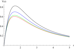
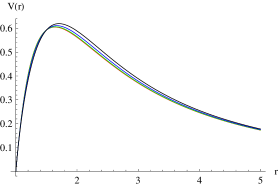
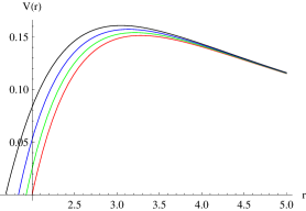
Figure 1: Effective potentials for various $\xi$ for the gravitational perturbations of the first (left), second (middle) and third (right) BH models. Here $M=1/2$ for the first and second models and $M=1$ for the third model, $\xi=0$ (red), $\xi=0.5$ (green), $\xi=1$ (blue), $\xi=1.5$ (black).

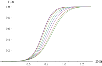
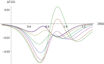
Figure 2: Right panel: Grey-body factors for various $\xi$ for the $\ell=2$ axial gravitational perturbations of the first BH model; the parameter $\xi=0.1$, $0.2$, $0.5$, $0.8$, $1$, $1.2$, $1.4$, $1.5$ from top to bottom, $M=1/2$. Left panel: difference between grey-body factors obtained by the 6th order WKB and the correspondence.

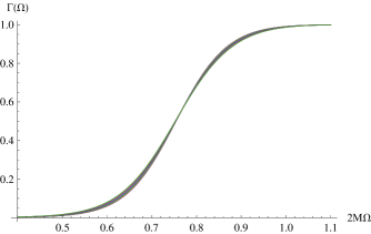
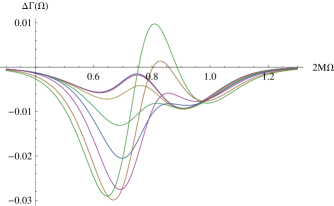
Figure 3: Right panel:Grey-body factors for various $\xi$ for the $\ell=2$ axial gravitational perturbations of the second BH model; the parameter $\xi=0.1$, $0.2$, $0.5$, $0.8$, $1$, $1.2$, $1.4$, $1.5$, $M=1/2$. Left panel: difference between grey-body factors obtained by the 6th order WKB and the correspondence.

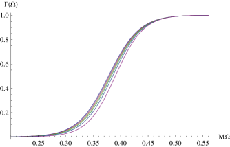
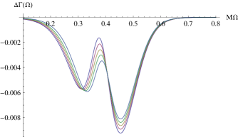
Figure 4: Right panel:Grey-body factors for various $\xi$ for the $\ell=2$ axial gravitational perturbations of the third BH model; the parameter $\xi=0.1$, $0.3$, $0.5$, $0.7$, $1$, $1.5$, $M=1$. Left panel: difference between grey-body factors obtained by the 6th order WKB and the correspondence.

III Grey-body factors obtained via the correspondence with quasinormal modes

In scattering processes around black holes, partial reflection of a wave by the potential barrier produces the same grey-body factors whether the wave originates near the horizon or arrives from infinity. This symmetry leads to boundary conditions defined as follows:

$$\begin{array}[]{rclcl}\Psi&=&e^{-i\Omega r_{*}}+Re^{i\Omega r_{*}},&&r_{*}\to+\infty,\\ \Psi&=&Te^{-i\Omega r_{*}},&&r_{*}\to-\infty,\end{array}$$ (7)

where $R$ and $T$ represent the reflection and transmission coefficients, respectively. In the context of black hole radiation, the transmission coefficient, $T$, is also referred to as the grey-body factor:

$$\Gamma_{\ell}(\Omega)=|T|^{2}=1-|R|^{2}$$ (8)

The general form for the quasinormal frequencies in the WKB approximation can be expressed as a series expansion around the eikonal limit, as follows [66]:

$$\omega^{2} = V_{0}+A_{2}({\cal K}^{2})+A_{4}({\cal K}^{2})+A_{6}({\cal K}^{2})+\ldots$$

$$- i{\cal K}\sqrt{-2V_{2}}\left(1+A_{3}({\cal K}^{2})+A_{5}({\cal K}^{2})+A_{7}({\cal K}^{2})+\ldots\right),$$

where $V_{0}$ is the potential at the peak, and $V_{2}$ is the second derivative of the potential with respect to the tortoise coordinate. Here, the terms $A_{i}({\cal K}^{2})$ denote higher-order WKB corrections. These corrections are explicitly detailed for the second and third WKB orders in [25], for the fourth through sixth orders in [26], and for orders up to the thirteenth in [67]. In the scattering problem, the WKB corrections are applied similarly, though the expression for ${\cal K}$ differs in accordance with the distinct boundary conditions.

The WKB method has been extensively developed and utilized across a wide range of studies [68, 42, 69, 70, 71, 72, 73], making it a robust tool for analyzing both quasinormal modes and grey-body factors. Given the wealth of literature on this subject, we will not delve into further details of the WKB method here.

The correspondence between the grey-body factors and quasinormal modes were derived for the spherically symmetric and asymptotically flat black holes via the WKB expression for the grey-body factors,

$$\Gamma_{\ell}(\Omega)=\dfrac{1}{1+e^{2\pi i{\cal K}}},$$ (10)

where [18]

$$i{\cal K}=\frac{\Omega^{2}-Re(\omega_{0})^{2}}{4Re(\omega_{0})Im(\omega_{0})}\Biggl{(}1+\frac{(Re(\omega_{0})-Re(\omega_{1}))^{2}}{32Im(\omega_{0})^{2}}$$

$$\qquad\qquad-\frac{3Im(\omega_{0})-Im(\omega_{1})}{24Im(\omega_{0})}\Biggr{)}-\frac{Re(\omega_{0})-Re(\omega_{1})}{16Im(\omega_{0})}$$

$$-\frac{(\omega^{2}-Re(\omega_{0})^{2})^{2}}{16Re(\omega_{0})^{3}Im(\omega_{0})}\left(1+\frac{Re(\omega_{0})(Re(\omega_{0})-Re(\omega_{1}))}{4Im(\omega_{0})^{2}}\right)$$

$$+\frac{(\omega^{2}-Re(\omega_{0})^{2})^{3}}{32Re(\omega_{0})^{5}Im(\omega_{0})}\Biggl{(}1+\frac{Re(\omega_{0})(Re(\omega_{0})-Re(\omega_{1}))}{4Im(\omega_{0})^{2}}$$

$$\qquad+Re(\omega_{0})^{2}\Biggl{(}\frac{(Re(\omega_{0})-Re(\omega_{1}))^{2}}{16Im(\omega_{0})^{4}}$$

$$\qquad\qquad-\frac{3Im(\omega_{0})-Im(\omega_{1})}{12Im(\omega_{0})}\Biggr{)}\Biggr{)}+{\cal O}\left(\frac{1}{\ell^{3}}\right).$$ (11)

Here $\omega_{0}$ and $\omega_{1}$ are, respectively, the dominant mode and the first overtone.

The grey-body factors are decreased when the quantum correction parameter $\xi$ is turned on (see figs. 2-4). This can be explained by the behaviour of the effective potentials: when $\xi$ is increased, the potential barrier is increased and the transmission coefficient becomes smaller. This behaviour can be easily seen for the first and third black hole models. The effective potential for second model depends only slightly on $\xi$. Therefore, the grey-body factors are almost unaffected by the quantum correction for that model.

An interesting example is given by the third black hole model for which the effective potential approaches the Schwarzschild one at a distance from the black hole, but drastically different in the near horizon zone. Overtones for this model experience an outburst, deviating from their Schwarzschild values at a speed increasing with the overtone number $n$. However, the grey-body factors are much less sensitive than overtones to the change of $\xi$, as seen in figs. 3, because grey-body factors depend only on the fundamental mode and the first overtone which deviate from their Schwartzschild limits only moderately.

However, grey-body factors can be calculated with greater precision using the higher order WKB expression for ${\cal K}$. The grey-body factors have been found in this way for various black holes and wormholes [74, 75, 36, 76, 77, 78, 49, 79, 80, 81, 82] and despite this is not exact expression for the quasinormal modes at finite $\ell$, we will use it to estimate the order of the relative error of the correspondence.

Comparison of the grey-body factors calculated via the 6th order WKB approach with those found through the correspondence with quasinormal modes shows that the difference ranges from a fraction of one percent to two-three percent depending on the value of $\xi$ and type of the black hole (see figs. 2-4). We have observed such a reasonable accuracy for the lowest multipole numbers $\ell=s$, where $s$ is the spin of the field. For larger $\ell$ the accuracy is even higher and usually do not exceed a small fraction of one percent.

IV Conclusions

Recently a correspondence between grey-body factors and quasinormal modes has been established [18]. This correspondence is precise in the eikonal limit, but its accuracy is, strictly speaking, unknown for finite $\ell$, due to asymptotic convergence of the WKB series. On the other hand, it was reported that unlike overtones of quasinormal modes, which are sensitive to small near horizon corrections [83], grey-body factors are much less sensitive to small corrections of the effective potential [16, 17]. Therefore testing the correspondence on metrics which deviate mainly in the near horizon zone is also testing the superior stability of the grey-body factors. The best choice for such metrics are various quantum corrected black holes. We used three recent models of such black holes to test the correspondence and showed that it holds with the remarkable accuracy for all of them. We have also confirmed that relatively small near horizon deformations, unless they also essentially change the geometry near the peak of the effective potential, do not lead to considerable shift in the grey-body factors.

- [1] S. W. Hawking. Particle Creation by Black Holes. Commun. Math. Phys., 43:199–220, 1975. [Erratum: Commun.Math.Phys. 46, 206 (1976)].
- [2] Don N. Page. Particle Emission Rates from a Black Hole: Massless Particles from an Uncharged, Nonrotating Hole. Phys. Rev. D, 13:198–206, 1976.
- [3] Don N. Page. Particle Emission Rates from a Black Hole. 2. Massless Particles from a Rotating Hole. Phys. Rev. D, 14:3260–3273, 1976.
- [4] Panagiota Kanti. Black holes in theories with large extra dimensions: A Review. Int. J. Mod. Phys. A, 19:4899–4951, 2004.
- [5] A. A. Starobinsky. Amplification of waves reflected from a rotating ”black hole”. Sov. Phys. JETP, 37(1):28–32, 1973.
- [6] Alexei A. Starobinskil and S. M. Churilov. Amplification of electromagnetic and gravitational waves scattered by a rotating ”black hole”. Sov. Phys. JETP, 65(1):1–5, 1974.
- [7] Jacob D. Bekenstein and Marcelo Schiffer. The Many faces of superradiance. Phys. Rev. D, 58:064014, 1998.
- [8] Theo Torres, Sam Patrick, Antonin Coutant, Mauricio Richartz, Edmund W. Tedford, and Silke Weinfurtner. Observation of superradiance in a vortex flow. Nature Phys., 13:833–836, 2017.
- [9] R. A. Konoplya. Magnetic field creates strong superradiant instability. Phys. Lett. B, 666:283–287, 2008.
- [10] Shahar Hod. On the instability regime of the rotating Kerr spacetime to massive scalar perturbations. Phys. Lett. B, 708:320–323, 2012.
- [11] William E. East and Frans Pretorius. Superradiant Instability and Backreaction of Massive Vector Fields around Kerr Black Holes. Phys. Rev. Lett., 119(4):041101, 2017.
- [12] B. P. Abbott et al. Observation of Gravitational Waves from a Binary Black Hole Merger. Phys. Rev. Lett., 116(6):061102, 2016.
- [13] B. P. Abbott et al. GW170817: Observation of Gravitational Waves from a Binary Neutron Star Inspiral. Phys. Rev. Lett., 119(16):161101, 2017.
- [14] Naritaka Oshita. Greybody factors imprinted on black hole ringdowns: An alternative to superposed quasinormal modes. Phys. Rev. D, 109(10):104028, 2024.
- [15] Kazumasa Okabayashi and Naritaka Oshita. Greybody factors imprinted on black hole ringdowns. II. Merging binary black holes. Phys. Rev. D, 110(6):064086, 2024.
- [16] Romeo Felice Rosato, Kyriakos Destounis, and Paolo Pani. Ringdown stability: greybody factors as stable gravitational-wave observables. 6 2024.
- [17] Naritaka Oshita, Kazufumi Takahashi, and Shinji Mukohyama. Stability and instability of the black hole greybody factors and ringdowns against a small-bump correction. Phys. Rev. D, 110(8):084070, 2024.
- [18] R. A. Konoplya and A. Zhidenko. Correspondence between grey-body factors and quasinormal modes. JCAP, 09:068, 2024.
- [19] R. A. Konoplya and A. Zhidenko. Correspondence between grey-body factors and quasinormal frequencies for rotating black holes. 8 2024.
- [20] R. A. Konoplya and A. F. Zinhailo. Quasinormal modes, stability and shadows of a black hole in the 4D Einstein–Gauss–Bonnet gravity. Eur. Phys. J. C, 80(11):1049, 2020.
- [21] R. A. Konoplya and Z. Stuchlík. Are eikonal quasinormal modes linked to the unstable circular null geodesics? Phys. Lett. B, 771:597–602, 2017.
- [22] S. V. Bolokhov. Black holes in Starobinsky-Bel-Robinson Gravity and the breakdown of quasinormal modes/null geodesics correspondence. Phys. Lett. B, 856:138879, 2024.
- [23] R. A. Konoplya. Further clarification on quasinormal modes/circular null geodesics correspondence. Phys. Lett. B, 838:137674, 2023.
- [24] Bernard F. Schutz and Clifford M. Will. Black hole normal modes - A semianalytic approach. Astrophys. J. Lett., 291:L33–L36, 1985.
- [25] Sai Iyer and Clifford M. Will. Black Hole Normal Modes: A WKB Approach. 1. Foundations and Application of a Higher Order WKB Analysis of Potential Barrier Scattering. Phys. Rev. D, 35:3621, 1987.
- [26] R. A. Konoplya. Quasinormal behavior of the d-dimensional Schwarzschild black hole and higher order WKB approach. Phys. Rev. D, 68:024018, 2003.
- [27] Milena Skvortsova. Quasinormal Spectrum of (2+1)-Dimensional Asymptotically Flat, dS and AdS Black Holes. Fortsch. Phys., 72(6):2400036, 2024.
- [28] Milena Skvortsova. Ringing of Extreme Regular Black Holes. Grav. Cosmol., 30(3):279–288, 2024.
- [29] Milena Skvortsova. Long Lived Quasinormal Modes of Regular and Extreme Black Holes. 2024.
- [30] Zainab Malik. Analytical QNMs of fields of various spin in the Hayward spacetime. EPL, 147(6):69001, 2024.
- [31] Zainab Malik. Quasinormal Modes of Dilaton Black Holes: Analytic Approximations. Int. J. Theor. Phys., 63(5):128, 2024.
- [32] Zainab Malik. Quasinormal Modes of the Bumblebee Black Holes with a Global Monopole. Int. J. Theor. Phys., 63(8):199, 2024.
- [33] Alexey Dubinsky. Quasinormal modes of charged black holes in Asymptotically Safe Gravity. Phys. Dark Univ., 46:101657, 2024.
- [34] Alexey Dubinsky and Antonina Zinhailo. Asymptotic decay and quasinormal frequencies of scalar and Dirac fields around dilaton-de Sitter black holes. Eur. Phys. J. C, 84(8):847, 2024.
- [35] K. D. Kokkotas, R. A. Konoplya, and A. Zhidenko. Quasinormal modes, scattering and Hawking radiation of Kerr-Newman black holes in a magnetic field. Phys. Rev. D, 83:024031, 2011.
- [36] Oleksandr Stashko. Quasinormal modes and gray-body factors of regular black holes in asymptotically safe gravity. Phys. Rev. D, 110(8):084016, 2024.
- [37] S. V. Bolokhov. Long-lived quasinormal modes and overtones’ behavior of holonomy-corrected black holes. Phys. Rev. D, 110(2):024010, 2024.
- [38] R. A. Konoplya and A. Zhidenko. Gravitational spectrum of black holes in the Einstein-Aether theory. Phys. Lett. B, 648:236–239, 2007.
- [39] Hideo Kodama, R. A. Konoplya, and Alexander Zhidenko. Gravitational stability of simply rotating Myers-Perry black holes: Tensorial perturbations. Phys. Rev. D, 81:044007, 2010.
- [40] M. A. Cuyubamba, R. A. Konoplya, and A. Zhidenko. Quasinormal modes and a new instability of Einstein-Gauss-Bonnet black holes in the de Sitter world. Phys. Rev. D, 93(10):104053, 2016.
- [41] Mahamat Saleh, Bouetou Thomas Bouetou, and Timoleon Crepin Kofane. Quasinormal modes of a quantum-corrected Schwarzschild black hole: gravitational and Dirac perturbations. Astrophys. Space Sci., 361(4):137, 2016.
- [42] E. Abdalla, R. A. Konoplya, and C. Molina. Scalar field evolution in Gauss-Bonnet black holes. Phys. Rev. D, 72:084006, 2005.
- [43] Cheng Liu, Tao Zhu, Qiang Wu, Kimet Jusufi, Mubasher Jamil, Mustapha Azreg-Aïnou, and Anzhong Wang. Shadow and quasinormal modes of a rotating loop quantum black hole. Phys. Rev. D, 101(8):084001, 2020. [Erratum: Phys.Rev.D 103, 089902 (2021)].
- [44] Jinsong Yang, Cong Zhang, and Yongge Ma. Shadow and stability of quantum-corrected black holes. Eur. Phys. J. C, 83(7):619, 2023.
- [45] Dhruba Jyoti Gogoi and Umananda Dev Goswami. Quasinormal modes and Hawking radiation sparsity of GUP corrected black holes in bumblebee gravity with topological defects. JCAP, 06(06):029, 2022.
- [46] R. A. Konoplya and A. Zhidenko. Eikonal instability of Gauss-Bonnet–(anti-)–de Sitter black holes. Phys. Rev. D, 95(10):104005, 2017.
- [47] Ramin G. Daghigh, Michael D. Green, and Gabor Kunstatter. Scalar Perturbations and Stability of a Loop Quantum Corrected Kruskal Black Hole. Phys. Rev. D, 103(8):084031, 2021.
- [48] M. B. Cruz, F. A. Brito, and C. A. S. Silva. Polar gravitational perturbations and quasinormal modes of a loop quantum gravity black hole. Phys. Rev. D, 102(4):044063, 2020.
- [49] R. A. Konoplya, D. Ovchinnikov, and B. Ahmedov. Bardeen spacetime as a quantum corrected Schwarzschild black hole: Quasinormal modes and Hawking radiation. Phys. Rev. D, 108(10):104054, 2023.
- [50] Hao Chen, Hassan Hassanabadi, Bekir Can Lütfüoğlu, and Zheng-Wen Long. Quantum corrections to the quasinormal modes of the Schwarzschild black hole. Gen. Rel. Grav., 54(11):143, 2022.
- [51] Cong Zhang, Jerzy Lewandowski, Yongge Ma, and Jinsong Yang. Black Holes and Covariance in Effective Quantum Gravity, arXiv: 2407.10168. 7 2024.
- [52] Jerzy Lewandowski, Yongge Ma, Jinsong Yang, and Cong Zhang. Quantum Oppenheimer-Snyder and Swiss Cheese Models. Phys. Rev. Lett., 130(10):101501, 2023.
- [53] Thomas Thiemann. Modern Canonical Quantum General Relativity. Cambridge University Press, Cambridge, UK, 2007.
- [54] Abhay Ashtekar and Jerzy Lewandowski. Background independent quantum gravity: A status report. Class. Quant. Grav., 21:R53, 2004.
- [55] Huajie Gong, Shulan Li, Dan Zhang, Guoyang Fu, and Jian-Pin Wu. Quasinormal modes of quantum-corrected black holes, arXiv: 2312.17639. 12 2023.
- [56] Milena Skvortsova. Quasinormal Frequencies of Fields with Various Spin in the Quantum Oppenheimer–Snyder Model of Black Holes. Fortsch. Phys., 72(9-10):2400132, 2024.
- [57] A. F. Zinhailo. Black Hole in the Quantum Oppenheimer-Snyder model: long lived modes and the overtones’ behavior, Research Gate preprint doi: 10.13140/RG.2.2.26785.01124. 2024.
- [58] Shu Luo. The quasinormal modes, pseudospectrum and time evolution of Proca fields in quantum Oppenheimer-Snyder-de Sitter spacetime. 8 2024.
- [59] Zainab Malik. Perturbations and Quasinormal Modes of the Dirac Field in Effective Quantum Gravity. 9 2024.
- [60] N. Heidari, A. A. Araújo Filho, R. C. Pantig, and A. Övgün. Absorption, Scattering, Geodesics, Shadows and Lensing Phenomena of Black Holes in Effective Quantum Gravity. 10 2024.
- [61] R. A. Konoplya and O. S. Stashko. Probing the Effective Quantum Gravity via Quasinormal Modes and Shadows of Black Holes. 8 2024.
- [62] Jerzy Lewandowski, Yongge Ma, Jinsong Yang, and Cong Zhang. Quantum oppenheimer-snyder and swiss cheese models. Physical Review Letters, 130(10), March 2023.
- [63] Kostas D. Kokkotas and Bernd G. Schmidt. Quasinormal modes of stars and black holes. Living Rev. Rel., 2:2, 1999.
- [64] Emanuele Berti, Vitor Cardoso, and Andrei O. Starinets. Quasinormal modes of black holes and black branes. Class. Quant. Grav., 26:163001, 2009.
- [65] R. A. Konoplya and A. Zhidenko. Quasinormal modes of black holes: From astrophysics to string theory. Rev. Mod. Phys., 83:793–836, 2011.
- [66] R. A. Konoplya, A. Zhidenko, and A. F. Zinhailo. Higher order WKB formula for quasinormal modes and grey-body factors: recipes for quick and accurate calculations. Class. Quant. Grav., 36:155002, 2019.
- [67] Jerzy Matyjasek and Michał Opala. Quasinormal modes of black holes. The improved semianalytic approach. Phys. Rev. D, 96(2):024011, 2017.
- [68] R. A. Konoplya. Quasinormal modes of the electrically charged dilaton black hole. Gen. Rel. Grav., 34:329–335, 2002.
- [69] Prosenjit Paul. Quasinormal modes of Einstein–scalar–Gauss–Bonnet black holes. Eur. Phys. J. C, 84(3):218, 2024.
- [70] Ramón Bécar, P. A. González, Eleftherios Papantonopoulos, and Yerko Vásquez. Massive scalar field perturbations of black holes surrounded by dark matter. Eur. Phys. J. C, 84(3):329, 2024.
- [71] Zhong-Wu Xia, Hao Yang, and Yan-Gang Miao. Scalar fields around a rotating loop quantum gravity black hole: waveform, quasi-normal modes and superradiance. Class. Quant. Grav., 41(16):165010, 2024.
- [72] Ahmad Al-Badawi. Probing regular MOG static spherically symmetric spacetime using greybody factors and quasinormal modes. Eur. Phys. J. C, 83(7):620, 2023.
- [73] Che-Yu Chen and Petr Kotlařík. Quasinormal modes of black holes encircled by a gravitating thin disk. Phys. Rev. D, 108(6):064052, 2023.
- [74] R. A. Konoplya and A. Zhidenko. Passage of radiation through wormholes of arbitrary shape. Phys. Rev. D, 81:124036, 2010.
- [75] Sharmanthie Fernando. Bardeen–de Sitter black holes. Int. J. Mod. Phys. D, 26(07):1750071, 2017.
- [76] Alexey Dubinsky and Antonina F. Zinhailo. Analytic expressions for grey-body factors of the general parametrized spherically symmetric black holes. 10 2024.
- [77] S. V. Bolokhov and R. A. Konoplya. Circumventing Quantum Gravity: Black Holes Evaporating into Macroscopic Wormholes. 10 2024.
- [78] R. A. Konoplya, A. F. Zinhailo, and Z. Stuchlik. Quasinormal modes and Hawking radiation of black holes in cubic gravity. Phys. Rev. D, 102(4):044023, 2020.
- [79] Bobir Toshmatov, Ahmadjon Abdujabbarov, Zdeněk Stuchlík, and Bobomurat Ahmedov. Quasinormal modes of test fields around regular black holes. Phys. Rev. D, 91(8):083008, 2015.
- [80] N. Heidari, H. Hassanabadi, A. A. Araújo Filho, J. Kříz, S. Zare, and P. J. Porfírio. Gravitational signatures of a non-commutative stable black hole. Phys. Dark Univ., 43:101382, 2024.
- [81] Julien Grain and A. Barrau. A WKB approach to scalar fields dynamics in curved space-time. Nucl. Phys. B, 742:253–274, 2006.
- [82] Sahel Dey and Sayan Chakrabarti. A note on electromagnetic and gravitational perturbations of the Bardeen de Sitter black hole: quasinormal modes and greybody factors. Eur. Phys. J. C, 79(6):504, 2019.
- [83] R. A. Konoplya and A. Zhidenko. First few overtones probe the event horizon geometry. JHEAp, 44:419–426, 2024.