Do Data Center Network Metrics Predict Application-Facing Performance?

Abstract.

Applications that run in large-scale data center networks (DCNs) rely on the DCN’s ability to deliver application requests in a performant manner. DCNs expose a complex design and operational space, and network designers and operators care how different options along this space affect application performance. One might run controlled experiments and measure the corresponding application-facing performance, but such experiments become progressively infeasible at a large scale, and simulations risk yielding inaccurate or incomplete results. Instead, we show that we can predict application-facing performance through more easily measured network metrics. For example, network telemetry metrics (e.g., link utilization) can predict application-facing metrics (e.g., transfer latency). Through large-scale measurements of production networks, we study the correlation between the two types of metrics, and construct predictive, interpretable models that serve as a suggestive guideline to network designers and operators. We show that no single network metric is universally the best predictor (even though some prior work has focused on a single predictor). We found that simple linear models often have the lowest error, while queueing-based models are better in a few cases.

1. Introduction

Large-scale applications are distributed across multiple machines in multiple racks, and thus their performance depends on behaviors, such as latency and throughput, of the data center networks (DCNs) where they run. These behaviors depend on multiple aspects of the underlying DCN, as well as the choices made by designers and operators.

We would like to evaluate how different aspects of network design and operation affect application performance. For example, when fabric planners are choosing between DCN designs, or provisioning DCN capacity, they want to know how their choices will affect application performance. Network operators need to know whether a DCN is reaching an operating point where application performance could be hurt. Traffic-engineering optimizers need network-level goals that preserve application performance. These use cases, and others, can depend on being able to predict application performance as a function of network behavior.

However, we cannot always make direct measurements of application performance, such as web page load times or banking transactions per second. The reasons include scale, data privacy, the intrusiveness of instrumenting applications to measure top-level (e.g., user-facing) performance, and our lack of knowledge of future workloads. Also, large-scale DCNs often support a complex mix of applications, which vary in how they use network, compute, and I/O.

Instead, we can leverage metrics that indicate when applications are bottlenecked by the DCN, such as flow completion times (FCTs), RPC latencies, and bulk-transfer goodput; we call these application-facing performance metrics (AFMs). We can then manage a DCN to preserve service-level objectives (SLOs) stated in terms of AFMs, under the reasonable assumption that this avoids DCN-bottlenecked applications (but we could not validate that assumption in this study).

This viewpoint converts our problem of directly predicting application performance into one of predicting AFMs from our knowledge of DCN design and workload characteristics, which is more practical but still difficult.

The gold-standard method to predict AFMs is to run controlled experiments, and then directly measure AFMs such as flow completion times. But those experiments are often infeasible: especially at scale, it can be difficult to replicate realistic application mixes and workloads, or even obtain the necessary hardware resources. Alternatively, we could actively perturb the network to discover how this affects a production workload, but the associated risks are usually unacceptable.

We could also run packet-level simulations based on application traces and record the simulated AFMs (e.g., (Zhang et al., 2021a; Zhao et al., 2023a)). However, simulations cannot always produce accurate results: First, simulators cannot always faithfully reflect the full complexity of a real DCN’s dataplane behavior. Second, realistic application traces are not always available, for reasons of scale or privacy. Third, traces capture application behavior under a specific set of network conditions, and might not represent behavior under different simulated conditions.

In this paper, we explore a different approach: we show how to create relatively simple and intuitive predictive models that relate AFMs to easily-measured network-level metrics (NLMs). Most production networks are already instrumented to collect NLMs, such as link utilizations and discard rates, via mechanisms such as sFlow, SNMP, or OpenConfig. Creating models that use NLMs to predict AFMs avoids the challenges of directly collecting application-facing metrics through expensive (or infeasible) experiments.

Using AFM and NLM traces for a large fraction of the applications in a set of production datacenters, we demonstrate that these models can indeed predict AFMs in many cases, with useful accuracy. They can also predict how operating a network in an overloaded regime can lead to unpredictable and hard-to-bound AFMs.

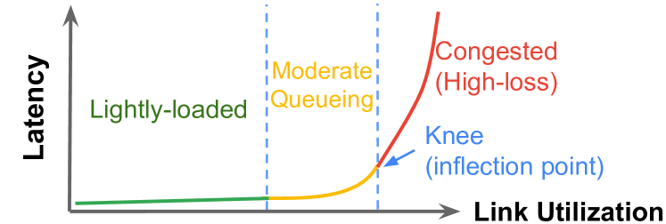
Figure 1. Hypothetical latency vs. link utilization.

We simplify the prediction challenge by considering network performance in three regimes (Figure 1) : lightly-loaded, where small changes in network metrics such as link utilization have little effect on AFMs; moderate-queueing, where changes in NLMs have significant but predictable impacts on AFMs; and congested, where large queuing delays and/or packet losses lead to severe and unpredictable application impacts. Stakeholders want to avoid the congested regime, and manage their tradeoffs within the other two regimes.

In our approach, we first model whether a network will be in the congested regime, by detecting knees in the curves representing AFM vs. NLM, via a modified version of the Kneedle algorithm (Satopaa et al., 2011) (§5.1). Our goal for this is not to predict application performance under severe congestion, but rather to predict when congestion will set in, so that this “danger zone” can be avoided.

Once we have identified the knee (if any), we then try to make predictions for the non-congested regimes. For these regimes, we create models using quantile regression (Koenker and Hallock, 2001) (§5.2, which exposes sensitivity in both linear (lightly-loaded) and non-linear (moderate-queueing) regimes of a network, and is robust to noise and outliers in the measurements. Users can add asymmetric bias §5.2.3) to steer results towards overprediction or underprediction.

This paper makes the following contributions:

• A method to produce trustworthy, actionable models that predict the relationships between a variety of AFMs and NLMs (§5). This methodology is transferable and can be applied by DCN designers and operators using their own datasets.

• An in-depth case study (§6) on a real-world fabric, validated on data from multiple production fabrics (§7).

• We identify which network metrics are good predictors, and show that NLMs and AFMs are correlated even in non-congested regimes.

• We further validate our approach on data from multiple production fabrics (§7).

• We empirically show that no single NLM is the best predictor for the AFMs studied (§6.2.1).

2. Background and Motivation

2.1. Data center network topology

Large-scale DCNs are typically designed to serve a diverse set of applications, with a goal of being agnostic to the application mix, since this can change. (Some DCNs are designed for specific large-scale applications, such as high-performance computing or machine-learning training; these single-function DCNs are outside the scope of this paper.)

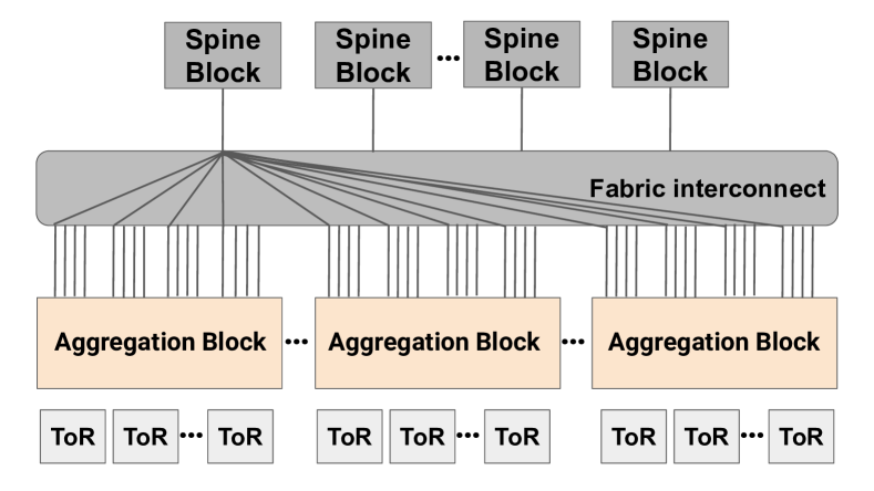
Figure 2. A typical Clos data center topology.

DCNs often rely on multi-path. multi-tiered topologies, such as Clos or Fat-Tree (Al-Fares et al., 2008), that provide a good balance of cost vs. performance for these application mixes. Fig. 2 shows a typical example, with three layers of switches: a Top-of-Rack (ToR) layer (to which machines are connected), an aggregation-block layer, and a spine-block layer. Aggregation and spine blocks are composed of several tiers of fully-connected switches.

While there are variations on this theme, such as Amazon’s (Callaghan and Rivers, 2022), the Facebook Fabric (Andreyev, 2014), or a spine-free Clos (Poutievski et al., 2022), the networks we study follow the design in Fig. 2.

2.2. Aspects of DCN performance

2.2.1. Expected vs. Realistic Behavior

While different applications have different network communication patterns, it has been shown that we can treat AFMs as simple functions of NLMs when the application is network-bottlenecked. For example, prior studies (Fortz and Thorup, 2000; Kumar et al., 2020; Zhang et al., 2021b) have shown that high link utilizations lead to higher discard rates, which would presumably lead to higher flow completion times (FCTs).

We might attempt to model the behavior of a network using queuing theory, but the complexities of real-network behavior does not always conform to simple models. At moderate utilizations, our results (Sections 6 and 7) are indeed consistent with modeling the DCN as a single, giant M/D/1 queue, which implies a reciprocal relationship between latency and utilization (Cooper, 2020). However, when the network is lightly loaded, with little or no persistent queueing, we often see a linear relationship between AFMs and NLMs; this is especially true for high-priority QoS (§2.2.2) classes that get preferential treatment. At high utilizations, packet losses due to full queues make queueing-theory models much harder to apply. Our goal is therefore to help stakeholders distinguish between these three operating regimes, and provide them with regime-specific predictive models, so that they can take appropriate actions.

2.2.2. Quality-of-service for Datacenter Applications

Large-scale DCNs often allow some applications to select Quality of Service (QoS) classes, giving their packets preferential treatment, to protect latency, loss, or throughput SLOs when link bandwidth or switch buffers are scarce. In this paper, we focus on three QoS classes:

• High priority: for applications that require low latency, and very low loss.

• Medium priority: for applications that accept some latency and a limited level of loss.

• Low priority: for applications that can tolerate more latency and/or more loss.

2.3. Application performance stakeholders

Various parties and systems would benefit from a deeper understanding of the relationship between NLMs and AFMs (the NLM-AFM relationship). These stakeholders are:

Fabric designers, who analyze competing DCN designs (e.g., (Al-Fares et al., 2008; Namyar et al., 2021; Poutievski et al., 2022; Zhao et al., 2023b)) to estimate their impacts on application performance. For example, designers often use forecasts of NLMs, such as expected utilization, to ensure sufficient capacity is built to serve the predicted demand (Gerstel et al., 2014; Zhu et al., 2021). Data on the NLM-AFM relationship gives a designer insights into which candidate designs are likely to support better application performance. E.g., if the switch hardware in an aggregation block is currently underprovisioned, leading to high utilization and reduced application performance, a designer can extrapolate from the NLM-AFM relationship to plan a cost-effective hardware upgrade that meets application needs. This might involve adding uplinks, or upgrading to switches with higher port speeds.

DCN operators, who would like to avoid application SLO violations based on definitions of different QoS classes and objectives. However, it is difficult to directly instrument the underlying applications due to privacy and scale issues. Understanding the NLM-AFM relationship helps operators detect signs of current or impending SLO violations, and allows them to implement corresponding mitigations, such as workload steering in the congested aggregation blocks.

Automated traffic and topology engineering systems that rely on network-level measurements to make reconfiguration decisions (e.g.,  (He et al., 2007; Kandula et al., 2005; Wang et al., 2006)). Traffic engineering (TE) is commonly used by large service providers to optimize traffic flowing through data centers and wide-area networks. State-of-the-art TE systems solve an optimization problem that decides how to split traffic through multiple paths for traffic demand between a given source and destination. The objective for this problem is typically a function derived from an NLM, with maximum link utilization (MLU) being the most commonly-used metric (Mitra and Ramakrishnan, 1999; Applegate et al., 2004; Agarwal et al., 2005; Wang et al., 2006; Poutievski et al., 2022). However, it is unclear how well MLU correlates to AFM performance, or whether MLU is the ideal NLM to optimize TE.

Topology engineering (ToE), which dynamically reconfigures capacity between aggregation block pairs to better match a non-uniform traffic demand, follows a similar form, where an optimization problem with an NLM-based objective is used to decide how to assign capacity between block pairs (Poutievski et al., 2022). Understanding the NLM-AFM relationship can help designers of these systems potentially choose optimization objectives that better reflect application-facing performance. For example, if a topology engineering system observes a network metric that exceeds a pre-defined threshold, and deduces that applications are at risk of SLO violations, the system can increase the network capacity between certain aggregation-block pairs.

Job schedulers, when choosing when to admit or place workloads, can leverage the NLM-AFM relationship to control rates at which hosts can send traffic into the DCN. For example, schedulers can place tasks or VMs to minimize congestion (Li et al., 2018), or temporarily throttle lower-priority flows to preserve high-QoS SLOs (Kumar et al., 2015; Perry et al., 2017).

Network researchers, who would like to know whether new network designs can better serve applications. It is difficult for academic researchers to gain access to large-scale workload traces and infrastructure that would allow them to directly measure application-facing performance. Knowing realistic NLM-AFM relationships would help researchers extrapolate application-facing behavior through network simulation, to validate their results.

2.4. Requirements of predictive models

All models are wrong, but some are useful.

George Box

Our models must be both actionable and as trustworthy as possible.

Actionable results allow stakeholders, such as designers and operators, to take appropriate measures to ensure application performance. To be actionable, model-based outputs must be interpretable in terms of application behavior, so that stakeholders can make straightforward decisions about network design and operation. We also need to differentiate between overprediction and underprediction of AFMs, because stakeholders generally need to bias these errors in one direction – when balancing application safety (SLO compliance) against infrastructure costs, most users treat SLO violations as the greater concern.

Stakeholders cannot rely on models that they do not trust. In particular, models need to be (1) robust against outliers, since measurements are usually noisy, and (2) provide confidence or error bounds, allowing users to understand the limits of trustworthiness, since most models are only reliable within certain ranges.

Our goal, therefore, is to provide models that accurately predict AFMs from NLMs when we have high confidence in those predictions, and to inform the user when we cannot provide a high-confidence model.

Some modeling methods fail to meet our requirements. For example, while machine learning has demonstrated robust predictive powers over various complex tasks (Zhu et al., 2021; Mao et al., 2019; Valadarsky et al., 2017), these black-box models do not provide interpretable predictions. Traditional regression methods are highly sensitive to outliers. High-fidelity simulations are not generally feasible at DCN scales. Real-world experiments, without some sort of model, are neither feasible nor predictive; an experiment can only tell us what happens under the tested conditions, not what might happen with a different network design or configuration. Table 1 summarizes these approaches.

	Requirement
Network Modeling Approach	Interpretability	Robustness	Error bounds	Realistic Scenarios
Deep Neural Networks	$\times$	✓	✓	✓
Regression	✓	$\times$	✓	✓
High-fidelity Simulations	$\triangle$	N/A	N/A	$\times$
Quantile Regression	✓	✓	✓	✓

Requirement satisfaction: ✓: full; $\triangle$: limited; $\times$: not met; N/A: not applicable for the approach.

Table 1. Comparison of NLM-AFM prediction approaches.

3. Methodology Overview

We now introduce a methodology that meets all the requirements above, by combing quantile regression and knee detection. Quantile regression simultaneously provides interpretability, robustness, error bounds, and also covers tail behavior and realistic scenarios. Knee detection provides an easily interpreted signal for when a network enters a highly-congested regime. This section briefly summarizes our approach. Subsequent sections develop each aspect in greater detail.

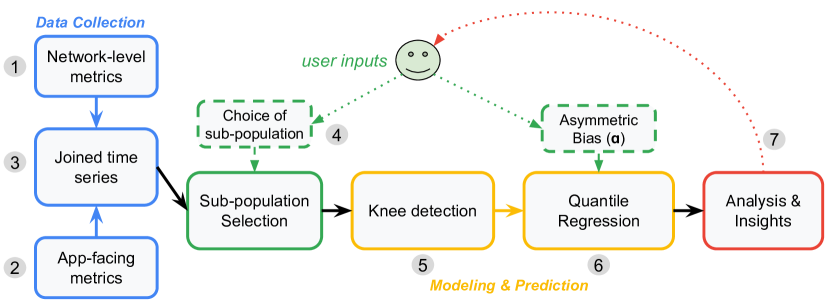
Figure 3. Overview of the approach

We start by gathering data for each DCN fabric of interest (§4.1), which allows us to make fabric-specific predictions. We currently treat each fabric as an independent prediction problem, because each fabric may have a unique mix of applications. For each fabric, we collect two datasets: time series of NLM metrics (§4.2, \small{1}⃝ in Fig. 3) and corresponding time series of AFM metrics (§4.3, \small{2}⃝). The NLM series come from standard switch-based network-monitoring sources, and cover all data-plane switches in these fabrics. The AFM series come from RPC-level instrumentation, and so these only cover the subset of applications which both use RPCs and allow us to instrument them. Aside from that limitation, the AFM traces are agnostic to application type.

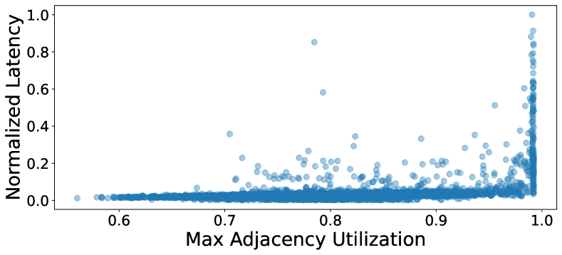
Max Adjacency Utilization is defined in Table 2

Figure 4. Example scatterplot of latency vs. utilization

Then, using the joined time-series datasets \small{3}⃝ for each fabric, the user may select a sub-population \small{4}⃝, such as the data for a specific QoS. We then analyze a number of pairwise data relationships between NLMs (such as link utilizations or discard rates) and AFMs (such as RPC latencies at different message sizes). It is helpful to visualize these pairs as scatterplots, with the NLM on the x-axis and the AFM on the y-axis; an example is shown in Fig. 4. For each such pair, we start by looking for “knees” – significant points of inflection – in the curve, using a modified version of the previously-published Kneedle algorithm (§5.1, \small{5}⃝). We assume these knees, if any, represent the transition to a congested regime; these become our predictions about where that transition will occur.

We then treat the data points to the left of a knee (if any) as representing the uncongested behavior of the fabric, and apply quantile regression to that subset of the data (§5.2, \small{6}⃝). Quantile regression is insensitive to outliers, and naturally provides confidence bounds for each prediction. Our approach to quantile regression supports both linear (lightly-loaded) and non-linear (moderate-queueing) behaviors, and how to distinguish between these regimes. It also supports user-tunable asymmetric bias, to favor SLO preservation over cost reduction (or vice versa).

Practical implications Network designers and operators, including automated control planes such as for traffic engineering, generally want to avoid congestion. Therefore, our ability to detect knees in the NLM-AFM relationship, if any, help to avoid these danger zones. For non-congested regimes, the results of quantile regression help designers and operators understand how application-facing performance might be affected by changes in NLMs \small{7}⃝.

When we have high confidence in a linear relationship, the slope provides a simple summary of the NLM-AFM relationship. When instead we have a high-confidence fit to a queueing-theory model, such as M/D/1, this suggests that relationship is reciprocal.

4. Data Collection Pipeline

This section describes the data we collected, both for developing our approach and for evaluating it.

4.1. Choice of fabrics

We collected NLM and AFM data for 19 different fabrics over a span of 2 months. These fabrics all use a Clos-like topology (Fig. 2) and serve generic applications. We choose the fabrics so that the value ranges of NLMs and AFMs we collect are as diverse as possible, allowing us to test our methodology over multiple regimes (lightly-loaded, moderate-queueing, and congested).

Note, however, that there is an inherent paradox in this dataset: our data comes from production workloads on production networks, but most production datacenter networks are carefully managed to avoid becoming performance bottlenecks. In particular, datacenter operators seldom allow significant congestion to persist, so we only have a few examples of highly-congested fabrics (i.e., where operators have determined that this is acceptable to users).

4.2. Network telemetry pipeline

In the fabrics we studied, the existing network-telemetry pipeline collects port-level switch statistics at 30-second intervals. This data covers switches at all layers (ToRs, aggregation blocks, and spine blocks) using a vendor-neutral industry-standard data model. Most enterprises have similar telemetry pipelines. Table 2 lists the metrics we considered in our analyses, including several metrics that we derive in a simple post-collection pass.

Table 2. Port-, link-, and adjacency-level metrics provided by our network telemetry pipeline.

Name Data Type Description Fabric Name Metadata Name of the fabric that contains the switch port. Stage Metadata Layer (i.e. ToR, aggregation, spine) where the switch is located. Port ID Metadata Port IDs of the switch and the peer switch. Port Speed Metadata Measured in bits per second. Src/Dst Aggregation Block Metadata Source and destination aggregation block containing the port. Total Octets Metric Sum of number of bytes that were received/sent at the port. Incoming Octets Metric Number of bytes that were received at the port. Outgoing Octets Metric Number of bytes that were sent at the port. Link Utilization Derived Sum of outgoing bits divided by port speed. Max/Average Link Utilization Derived Max/Average link utilization across all links in the fabric. k-th Percentile Link Utilization Derived The k-th percentile link utilization across all links in the fabric. P5-P95 distance: Link Util. Derived The difference between the 5th and 95th percentile link utlization. Adjacency Utilization Derived Sum of outgoing bits divided by port speed. Max/Average Adjacency Utilization Derived Max/Average adjacency utilization across all links in the fabric. k-th Percentile Adjacency Utilization Derived The k-th percentile adjacency utilization across all links in the fabric. P5-P95 distance: Adjacency Util. Derived The difference between the 5th and 95th percentile adjacency utlization.

By exploiting metadata, such as the prefixes of chassis names, we have the flexibility to group the network data at various granularities. We can look at individual link-level statistics – e.g., basing a prediction on the most-utilized link between a pair of blocks – or we can analyze aggregations of links, formally defined as adjacencies – e.g., treating all links between a pair of blocks as a single aggregated link. Coarse-grained, adjacency-level utilization exposes fabric-wide behavior, while fine-grained, port-level link utilization exposes outlier behaviors within the fabric.

4.3. RPC instrumentation

A large fraction of the traffic in the fabrics we studied comes from RPC-based applications. The RPC layer used in most of these applications includes transport-level instrumentation, RPCAFMs (similar to Fathom (Qureshi et al., 2023)), that passively collects some AFMs.

RPCAFMs breaks down each RPC into a set of events, each associated with high-resolution kernel timestamps as the RPC requests and responses traverse the stack. This allows RPCAFMs to collect both message-oriented metrics, such as RPC transmit latencies, and connection-oriented metrics, such as delivery rates (bytes/sec). Table 3 lists the metrics that we use in this paper.

Table 3. RPC metrics collected

Name Data Type Description Transmit Latency Message-Oriented Metric Time from when the first byte is sent to a NIC to when an ACK is received for a prefix of the message. Values are separately measured for small, medium and large RPCs. Delivery Rate Connection-Oriented Metric Non-application-limited throughput of the connection. Traffic Class Metadata The traffic class (i.e. QoS class) of the issued RPC. Congestion Control Metadata The underlying congestion control algorithm used in the TCP connection. Src/Dst Aggr. Block Metadata The source and destination aggregation blocks of the RPC request.

To avoid the computational and storage demands from saving raw data on billions of RPCs issued daily in our fabrics, RPCAFMs leverages t-digests (Dunning and Ertl, 2019). T-digests preserve the original distribution of the data through approximated quantiles. Compared to other compression methods, such as binning with histograms, the t-digest data structure has high approximation accuracy, especially at the tail, and can be merged with other independent t-digests (e.g. through common SQL operations like “GROUP BY”). Based on the calculated t-digests, we summarize the RPC metrics into different percentiles of the metrics’ distribution. We can also group the derived t-digests based on different AFM attributes to support a wide range of analyses.

To further reduce overhead, RPCAFMs reports data aggregated over 5-minute intervals, so when we join this data with NLM data, we also re-aggregate the NLM data over 5-minute intervals. We would prefer to use shorter intervals, but this tradeoff is currently necessary for feasibility.

Note that, because RPCAFMs was designed for a different purpose and to execute with minimal impact on applications, the way it reports data grouped by RPC sizes is a little unusual. For example, for message lengths between 1 KiB and 8 KiB, RPCAFMs reports transmit latency from when the first byte is handed to the NIC until TCP receives the acknowledgement for the last byte of the first 1 KiB of the message. (See Fig. 21.) Similarly, for messages between 64KiB and 256KiB, latency is measured for the first 64KiB. This is therefore (1) not the same thing as the round-trip RPC latency, since it measures each direction of an RPC independently, and (2) only measures transmit latency for a prefix of the message. However, we believe that RPCAFMs-based AFMs are a reasonable proxy for actual application-facing network performance.

Enterprises without a system like RPCAFMs might instead use mechanisms such as DTrace (Cantrill et al., 2004) to collect AFMs.

5. Methodology and algorithms

Our methodology incorporates two components: knee detection with Kneedle, and quantile regression. The Kneedle algorithm, based on geometry theory, detects whether AFMs experience congestion after a certain NLM threshold. Quantile regression provides statistical predictions of the NLM-AFM relationship, with strong noise/outlier resistance.

5.1. Knee Detection with Kneedle

The “knee” of a curve is a point where the slope of a curve changes suddenly – i.e., has a high second derivative. In the analysis of computer system performance, a knee in the relationship between an independent variable (e.g., an NLM) and a dependent variable (e.g., an AFM) often represents a transition from “good” to “bad” behavior. In packet networks, this typically represents a transition to a congested regime. Therefore, we would like to predict whether an AFM-vs-NLM relationship has knee, and if so, where it is.

One challenge is that the definition of a “knee” is informal and heuristic, and can vary dramatically depending on application-specific objectives and the chosen coordinate scales. We believe the concept is still useful, since it aligns well with an intuitive explanation of network behavior – for example, the rapid increase in RPC tail latency that occurs above a threshold network utilization.

For knee detection, we use the previously-published Kneedle algorithm (Satopaa et al., 2011). Kneedle formalizes the intuitive notion of knee as the point of maximum curvature in a function (i.e., its deviation from a straight line). A potential knee is defined as the $x$ value where there is local-maximum curvature.

Kneedle operates on a curve, not on a set of (NLM, AFM) samples, so we define the envelope of a dataset as the 95th percentile AFM value in each of $k$ buckets across the dataset. (This captures the bulk of the dataset without being too sensitive to outliers.) We chose $k$ to match the number of buckets appropriate to the x-axis extent of the data; see §6.1 for how we do that. These choices are somewhat arbitrary, but we found that algorithm finds almost the same knees no matter what percentile we used. Because knee-detection is inherently use-case-specific, we modified the Kneedle algorithm’s criteria for finding a knee in two ways:

1. Curvature of the potential knee is larger or equal to threshold $\mathcal{C}$. Not all AFM-NLM metrics have interesting knees; we only want to find points that represent drastic degradation in the AFM. Therefore, we enforce a minimal threshold $\mathcal{C}$ for the curvature of a detected knee. In comparison, vanilla Kneedle returns the point of maximum curvature as the knee, regardless of its absolute value. $\mathcal{C}$ is adjustable based on the risk tolerance of operators.

2. Curvature of the detected knee is a global maximum. We would like to avoid any local maxima, which can result from minor measurement noise, and so we only return the worst (maximum-curvature) knee.

The Kneedle algorithm also requires users to specify the convexity/concavity of the relationship, and assumes that the relationship is strictly increasing or decreasing. While we expect some behavioral deviations from the ideal NLM-AFM relationship (§2.2.1) due to measurement noise and other potential factors, we generally observe a reliably convex relationship between NLMs and latency-based AFMs. This pattern emerges as the data center network behaves like a large-scale queueing system, formed by collective buffers of network switches. Queueing theory predicts that delay in such systems follows a convex relationship. Conversely, we assume a concave relationship between NLMs and throughput-based AFMs, where we expect per-application/RPC throughput to decrease as the network becomes increasingly saturated.

In a few cases, Kneedle finds a false knee, either much smaller than the “true” knee, or when there is no clear knee at all. We might be able to improve the algorithm to avoid that; this is future work.

5.2. Quantile Regression

For NLM-AFM relationships to the left of a knee, or where there is no clear knee, we use regression analysis to provide a simple predictive model for AFMs. For this, we use quantile regression (Koenker and Hallock, 2001), a type of regression analysis that estimates the quantiles (e.g. the median, the 90th percentile, etc.) of a target variable. This differs from classical regression models that directly predict the target variable.

Quantile regression provides two advantages over classical regression models: (1) quantile regression is extremely robust to noise, because a small number of outlier values have minimal effect on the calculated quantiles; and (2) with quantile regression, we can inspect different quantiles of the same dataset, to obtain a more well-rounded view of the data (e.g., by looking at both median and tail percentiles of a target variable). We can apply quantile regression both for linear models (e.g., for lightly-loaded network regimes), and for non-linear models (e.g., for moderate-queuing regimes); we discuss the latter in §5.2.4.

To provide a brief overview of quantile regression’s formulation, we use a linear model as an example. Consider a classical linear regression formulation, with a single predictor variable ($x$) and a single target variable ($y$):

(1) $$y=\beta x+c$$

$\beta$ is known as the slope, and $c$ is known as the intercept of the equation. We can interpret Eq. 1 as the expected change in y per unit change in x. In linear quantile regression, instead of estimating the expected change in the y value, we estimate the $\tau$-th percentile of $y$, where $\tau$ ($0\leq\tau\leq 1$) is defined as the probability that the targert variable $y$ is smaller or equal to $\mu_{\tau}$, the $\tau$-th percentile of $y$.

(2) $$\tau=Pr(y\leq\mu_{\tau})\equiv F_{y}(\mu_{\tau})$$

(3) $$\mu_{\tau}=F_{y}^{-1}(\tau)$$

We can then define the conditional quantile of $y$ as:

(4) $$y_{\tau|x}=\mu_{\tau|x}=F_{y|x}^{-1}(\tau|x)=\beta x+c$$

where conditioning on $x$ produces $(x,y_{\tau})$ pairs that can then be modeled using common regression techniques.

5.2.1. Data Discretization

As shown in Equation 4, $y_{\tau|x}$ conditions quantile values of $y$ on certain values of $x$. If we have the ground-truth distribution of the underlying $x,y$ relationship, we can directly calculate $\mu_{\tau}(x)$ through its PDF. However, we seldom have the ground truth of the actual distribution. Instead, we typically have a series of $(x,y)$ data points, which are then used to estimate the ground truth of the distribution. In order to approximate the conditional quantiles, in quantile regression the predictor variable $x$ is first bucketed into equal-sized buckets. Then, the conditional quantile $y_{\tau}=\mu_{\tau}(x)$ is taken based on each respective bucket. This allows quantile regression to operate on observed data and construct predictive models.

5.2.2. Targeted Quantiles

One strength of quantile regression is its ability to look at different quantiles of the dataset. In this paper, we focus on constructing models for the 95th percentiles of the collected latency-related measurements to cover broad aspects of (NLM, AFM) performance. (A higher percentile means that a model explains more of the worst-case data. Ideally we could present 99th percentile data, but with our current 5-minute sample windows, many buckets do not contain sufficient samples to compute that percentile.) We refer to the model fitted to the 95-th quantile of each network-metric bucket as the ‘95th quantile regression’ model, or QR95 for short. (§C shows an example of how different quantiles lead to different models.)

For delivery-rate AFMs, since SLOs focus on worst-case behavior, we collected the p1 rates (i.e, worse than 99% of the samples) and then fit models to the 5th percentile of the measured p1 rates, not the 95th.

5.2.3. Asymmetric Bias

During training (model creation), we want to allow users of our methodology to tune its objective towards overprediction or underprediction, depending on their understanding of relative risk. Therefore, instead of traditionally symmetric, least-square-based estimation methods, we introduce an asymmetric form of the least-squares objective (inspired by the formulation in  (White, 2020)). Specifically, we define the asymmetric mean squared error (AMSE) as:

(5) $$\small\begin{split}AMSE=2\Big{(}\alpha\frac{1}{N_{o}}\sum_{i=1}^{N_{o}}[\max(0,f(x_{i})-y_{i})]^{2}\\ +(1-\alpha)\frac{1}{N_{u}}\sum_{i=1}^{N_{u}}[\min(0,f(x_{i})-y_{i})]^{2}\Big{)}\end{split}$$

where $y_{i}$ is the ground truth of the target variable, $f(x_{i})$ is the model prediction, $N_{o}$ is the number of samples the model overpredicted, and $N_{u}$ is the number of samples the model underpredicted. $\alpha$ is an adjustable weight that allows the regression model to favor overprediction or underprediction during training. When $\alpha$ is larger 0.5, AMSE penalizes overprediction more; where overpredicted samples are captured by the $max$ term, and vice versa. AMSE falls back to symmetric least-squares when $\alpha=0.5$.

When evaluating a predicted model against test data, we wanted a normalized metric, so we use the relative, square-rooted form of AMSE, relative asymmetric root mean squared error (rARMSE). Taking the root of the squared error makes rARMSE have the same units as the target variable and easier to interpret the magnitude of the prediction errors. Calculating the error as a ratio (with denominator $y_{i}$) makes the error scale-independent, allowing it to be applied across different AFMs without setting specific error thresholds for each individual AFM. rARMSE can be written as:

(6) $$\small\begin{split}rARMSE=2\Big{(}\alpha\frac{1}{N_{o}}\sum_{i=1}^{N_{o}}[\max(0,(f(x_{i})-y_{i})/y_{i})]^{2}\\ +(1-\alpha)\frac{1}{N_{u}}\sum_{i=1}^{N_{u}}[\min(0,(f(x_{i})-y_{i})/y_{i})]^{2}\Big{)}^{\frac{1}{2}}\end{split}$$

5.2.4. Linear and Non-linear quantile regression

We choose to fit (NLM, AFM) relationships on both a linear model and a queueing (M/D/1) model to reflect the lightly-loaded and moderate-queuing regimes of a network (Figure 1). We perform quantile regression twice, once on each model, and choose the model with the lowest AMSE.

For an M/D/1 queue, service delay (such as transmit latency) and utilization follow a reciprocal relationship (Cooper, 2020). When fitting our data to an M/D/1 model, we first perform feature transformation based on Equation 7. Feature transformation allows us to treat non-linear models as if they are using linear features, allowing us to solve as linear regresssions, which is more efficient. Note that linearity is considered with respect to the original features or with respect to the transformed features, whereas the queueing theory-based model assumes a non-linear relationship between utilization and delay.

(7) $$Percentile_{\tau}(y)=\beta\frac{x}{1-x}+c=\beta Q+c$$

5.3. Combined algorithms

To combine Kneedle and quantile regression, for each (NLM, AFM) pair of interest, we derive a predictive model by:

1. Applying the Kneedle algorithm to detect and record a knee, if any.

2. If there is a knee, creating a subset of the data points for which the NLM is smaller than one bucket before the knee, to ensure that there are no false negatives due to bucketization. If there is no knee, use the entire dataset as this subset. (The offset of one bucket is arbitrary, but appears to work.)

3. For the subset of (NLM, AFM) pairs selected in the previous step, we perform quantile regression twice, using both linear and queueing-theory models.

4. We report the model (linear or queueing theory) with the lowest rARMSE. If no models have a confidence score above a threshold (§8.1), we assume that the (NLM, AFM) pair has no clear relationship.

Understanding model stability: The best model for a given fabric might vary over time. To understand this variability, we can derive a model (for a given NLM-AFM pair) using a subset of the input data covering time spans of various durations, and then validating these models against held-back data from other time spans, i.e. splitting the input data into training and testing sets. This helps network designers and operators understand how frequently they would need to update their predictive models, to avoid stale results.

Our methodology combines a data-driven approach that utilizes training and testing sets, with an analytical framework based on queueing theory models. The key insight to this combined learning-based + analytical model approach is that we can adapt certain predictive models (e.g. the M/D/1 queueing model) that are informed by domain-specific knowledge of network behavior, instead of using generic regression techniques or deep neural networks. On the other hand, the integration of data-driven techniques then ensures that our predictive models remain robust to changes in NLM/AFM patterns, remaining practical and actionable for network operators in real-world scenarios.

6. Production Fabric Case Study

Before presenting a broad analysis across 19 production fabrics, code-named $A..S$, in §7, we present an in-depth analysis of fabric C, which contains 51 active aggregation blocks. We chose C because its operators have chosen to allow several aggregation blocks to run at persistent high utilizations, and so this fabric illustrates several interesting aspects of our methodology.

For fabric C we looked at how well we can build predictive models (via training and testing), whether the choice of model (linear or queueing-based) is stable from week to week, and which NLMs are the best predictors. We present results for both low-QoS and medium-QoS flows; the fabric preserves sufficient bandwidth for high-QoS flows that these results are uninteresting (i.e., they always perform well). We looked at both NLMs representing inter-aggregation-block links and aggregated adjacencies (§6.2) and per-block NLMs representing intra-block links (§6.3).

We aim to answer the following questions:
Q1: Is it feasible to create fabric-wide predictions? (i.e., using NLMs that represent fabric-wide network performance) (§6.2)
Q2: Which NLMs are good predictors, and are the same NLMs good predictors in all cases? (§6.2.1)
Q3: Is the best choice of models stable over periods of weeks or longer? (§6.2.2)
Q4: In which circumstances are linear or queuing-based models better predictors? (§6.2.2)

We chose to analyze these NLMs:

• Link Utilization: utilization, measured over one sample period (5 minutes) of a given link.

• Maximum Link Utilization (MLU): maximum, during one sample period, of all link utilizations in the fabric.

• Average Link Utilization (ALU): average, during one period, of all link utilizations in the fabric.

• Adjacency Utilization: utilization aggregated over all links between a pair of blocks.

• Maximum Adjacency Utilization (MAU): maximum, during one sample period, of all adjacency utilizations in the fabric.

• Average Adjacency Utilization (AAU): average, during one period, of all adjacency utilizations in the fabric.

• Jain: Jain’s fairness index (Jain et al., 1984), computed over the set of link utilizations, as a proxy for “load imbalance” across those links.

• P5-P95-distance: difference between the 5th and 95th percentile link utilizations (an alternate measure of imbalance).

These metrics are derived from the metrics and metadata summarized in Table 2.

6.1. Model-training and testing parameters

Our dataset covers two months. For most of these results, we trained models on 4 weeks of data, and tested them on data from the following 2 weeks. We split the NLM data into 20 buckets (5%/bucket) for maximum utilizations, and into 100 buckets (1%/bucket) for mean utilizations, since the latter datasets had smaller domains, and we needed smaller buckets to have enough that contained sufficient samples. For knee detection, we set the curvature threshold $\mathcal{C}=0.5$. We declared a model to be “accurate” during testing if the $rARMSE<0.15$. §8.1 discusses the choice of this threshold.

Throughout this section, we present QR95 results, as defined in §5.2.2, unless otherwise noted.

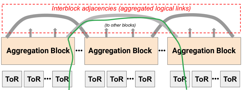
Green line shows path of an inter-block RPC

Figure 5. Links used for inter-block NLMs

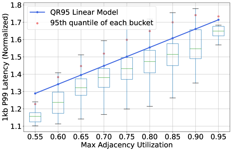
Figure 6. Fabric C, 64kb Tail Transmit Latency, medium QoS, NLM $=$ MAU.

6.2. Fabric-wide (inter-block) predictions

In this section, we look at AFMs for RPCs that cross between aggregation blocks, using NLMs only from the aggregated links (“adjacencies”) between blocks, as illustrated in Fig. 6.

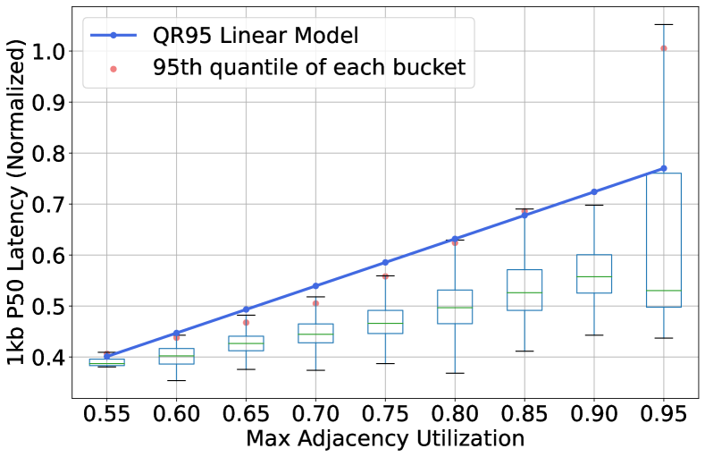
(a) 1kb Median Transmit Latency.

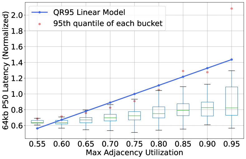
(b) 64kb Median Transmit Latency.

Figure 7. Fabric C models: p50 AFMs, low QoS, NLM $=$ MAU.

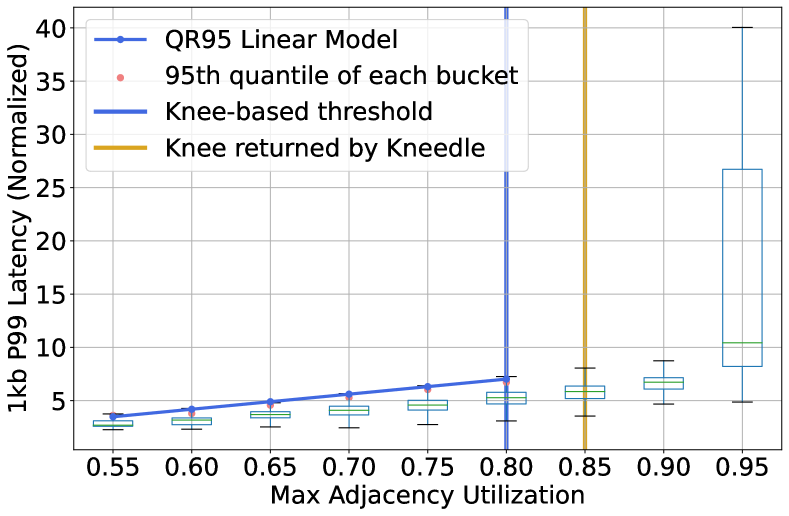
(a) 1kb Tail Transmit Latency.

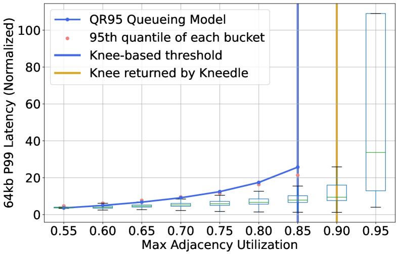
(b) 64kb Tail Transmit Latency.

Figure 8. Fabric C models: p99 AFMs, low QoS, NLM $=$ MAU.

Figures 7 and 8 present detailed results for low-QoS flows (the QoS most affected by network utilization). These and all similar figures are normalized to consistent but arbitrary baselines. Both show results using MAU as the NLM predictor (§6.2.1 discusses other NLMs). These graphs show box plots of the underlying test data, vertical lines for the upper limit of the regression subset (see §5.3), and curves for the linear or queueing-based models we predicted.

Fig. 7 shows that for p50 (median) AFMs, we obtain good fits with linear models. Fig. 8 shows that for p99 (tail) AFMs, a queueing-based model is a much better fit, and that AFMs increase rapidly after the knees.

We did not detect any knees for medium-QoS flows, likely because the network sufficiently protects these flows. Fig. 6 illustrates this for median-QoS RPC tail latency.

Note that we tried training models on data grouped by congestion-control algorithm (CCA), since different flows in our dataset use different CCAs, but this did not lead to accurate models. For various other AFMs, such as the number of timeouts, we could not construct high-confidence models. In a well-managed network, these events are rare, even at high utilization.

6.2.1. Best NLMs

For Fabric C, different NLMs provide the highest prediction accuracy (lowest error) in different cases. Maximum adjacency utilization (MAU) was consistently the best predictor for low-QoS traffic, but generally had poor accuracy for high-QoS traffic (possibly because, for high QoS, end-host delays rather than network delays, dominate (Agarwal et al., 2022)). Medium-QoS AFMs were best predicted by MAU, except that P95_P5_dist was a slightly better predictor, than MAU, for 64kb-RPC median latencies.

In §7.1, we plot accuracies across multiple fabrics, and show that for a given AFM, the NLM that yields the lowest prediction error changes fabric-to-fabric.

6.2.2. Stability

Prediction stability. Ideally, models would be stable over time – i.e., a model that worked during the most recent two weeks (linear or queueing) would still work for the next two weeks. To evaluate stability, we applied a sliding window, where we trained a new model starting every two weeks, using four weeks of training data, and tested it on the fifth and sixth week’s data. We used an additional month of Fabric C data to obtain sufficient results for four consecutive windows.

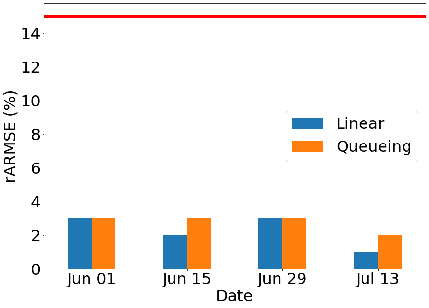
(a) 1kb RPC Latency, P50.

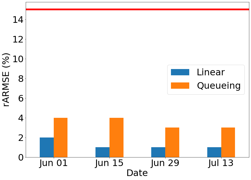
(b) 64kb RPC Latency, P50.

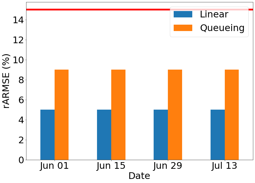
(c) 1kb RPC Latency, P99.

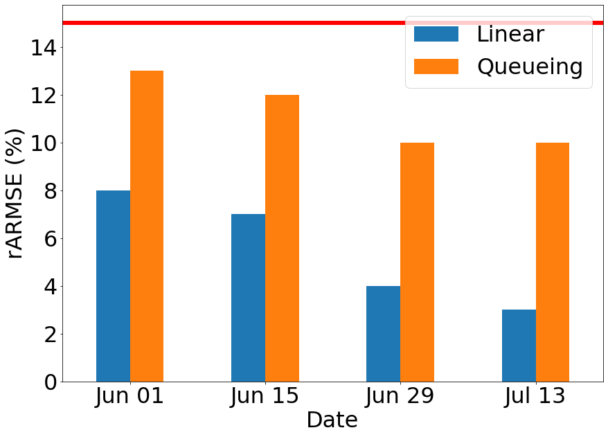
(d) 64kb RPC Latency, P99.

Red line indicates the rARMSE threshold ($15\%$). NLM $=$ MAU in these graphs

Figure 9. Week-to-week stability, medium-QoS flows.

Fig. 9 shows the corresponding results for medium-QoS flows. These predictions are more stable and generally more accurate than those in Fig. 10 – always well within our 15% threshold – and the linear model is consistently more accurate than the queueing-based model, presumably because the medium-QoS flows are less likely to experience queueing.

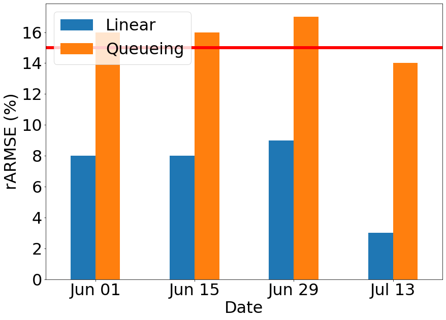
(a) 1kb RPC Latency, P50.

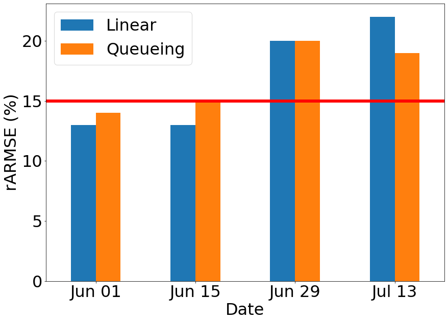
(b) 64kb RPC Latency, P50.

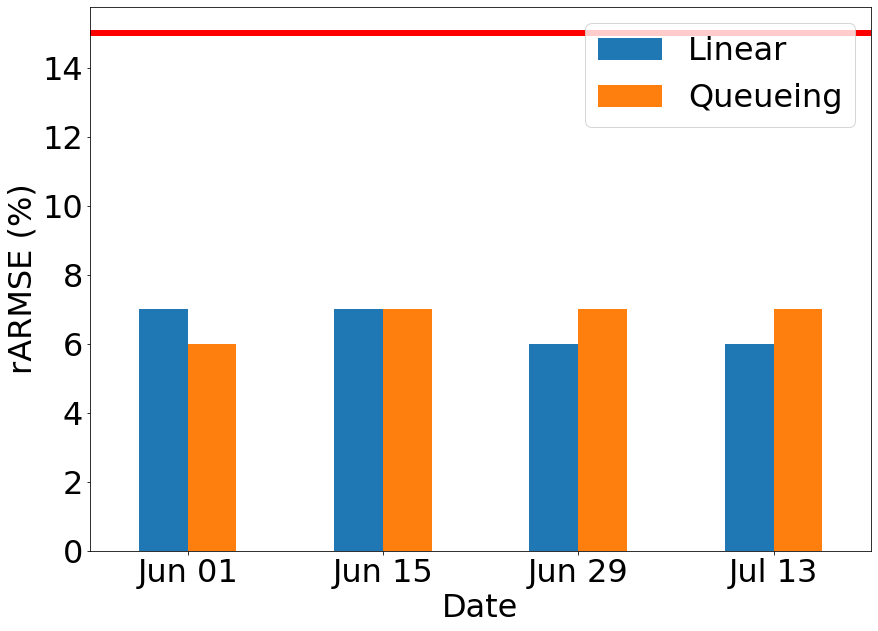
(c) 1kb RPC Latency, P99.

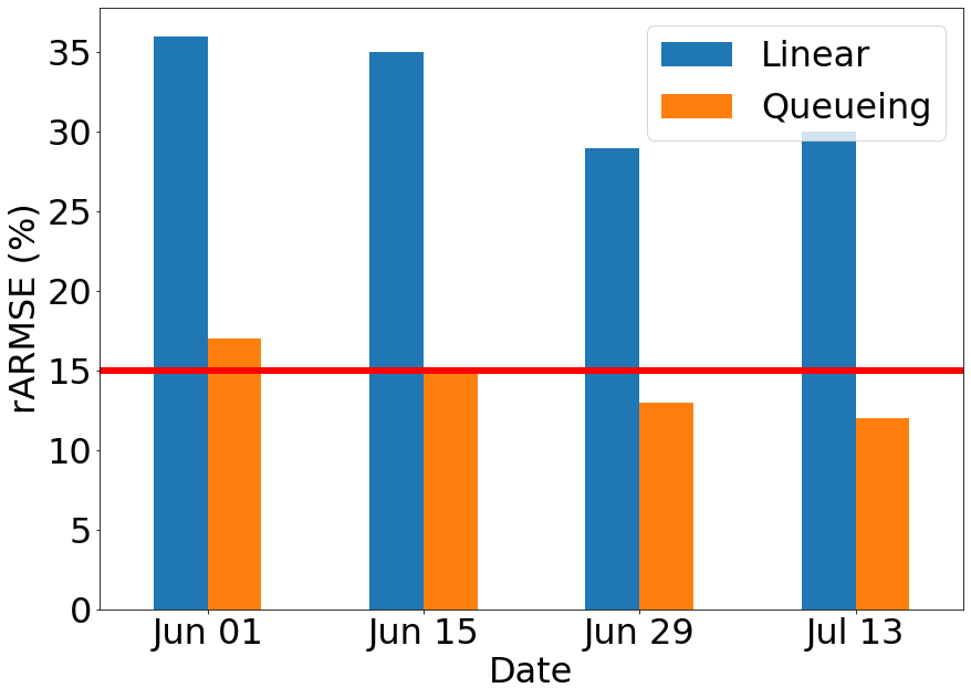
(d) 64kb RPC Latency, P99.

Red line indicates the rARMSE threshold ($15\%$). NLM $=$ MAU in these graphs

Figure 10. Week-to-week stability, low-QoS flows.

Fig. 10 shows that, for low-QoS flows, our algorithm consistently chooses a linear model for small-RPC p50 latency (Fig. 10(a)). It consistently chooses a queueing model for large-RPC p99 latency (Fig. 10(d)), presumably because large RPCs take more round trips to complete, so DCN conditions are more likely to trigger congestion-avoidance mechanisms. For large-RPC p50 (Fig. 10(b)) and small-RPC p99 (Fig. 10(c)) AFMs, neither model consistently “wins.” However, in most cases, we can find a model that meets our 15% error threshold.

Knee stability. In cases where we detect a knee, is the knee stable? We applied a one-week sliding window, across 6 weeks, to see if knees appear, disappear, or change position between weeks.

Indeed, in most cases for this fabric (for both small and large RPC latencies) for P99 AFMs for low-QoS flows, the knees we detected were stable at MAU=90%. In one case (July 6, small RPC latencies) the knee moved to MAU=95%; this could be a bucket-quantization effect. For delivery rates, we found a knee only for the week of July 6.

6.3. Block-level Predictions

In this section, we look at AFMs for RPCs that stay within aggregation blocks, using NLMs only from the individual (non-aggregated) internal links within each block, as illustrated in Fig. 12. Note that we do not include NLMs from ToR uplinks or downlinks.

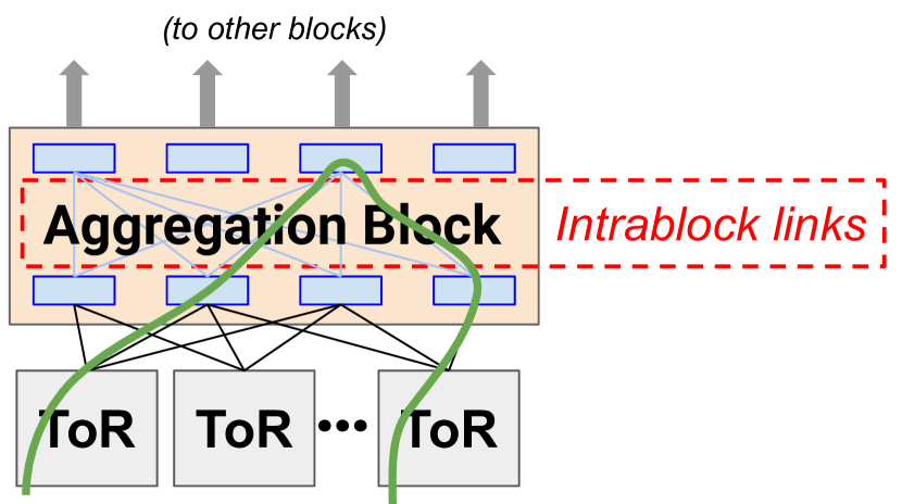
Green line shows path of an intra-block RPC.

Figure 11. Links used for intra-block NLMs

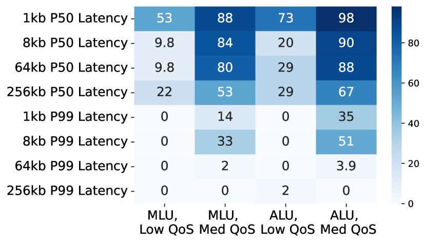
Cells $=$ % of all aggregation blocks with models with $rARMSE\leq 0.15$.

Figure 12. Frequency of agg. blocks w/ accurate models.

Figure 12 shows, for each AFM, the percentage of aggregation blocks, in fabric C, for which we obtained high-accuracy models. The figure shows results for two NLMs, average link utilization and maximum link utilization; and for both low-QoS and medium-QoS flows.

These results show that, for flows within an aggregation block, medium-QoS latency is far more predictable than low-QoS latency; small-RPC latency is usually easier to predict than large-RPC latency; and median latency is easier to predict than tail latency. They also show that ALU is always (for this dataset) a better predictor than MLU.

7. Multi-fabric analysis

In this section, we present results across all 19 production fabrics in our dataset, to understand if the results in §6 generalize. Specifically,

• What are the NLMs with the highest prediction accuracy? Is it consistent across fabrics? (§7.1)

• Can we accurately predict AFMs over all fabrics or some of them? (§7.1)

• Are linear or queueing models consistently better across all fabrics? (§7.2)

• What fraction of the data is covered within the knee-based thresholds? (§7.3)

§E extends the block-level analysis of §6.3 to multiple fabrics.

7.1. Fabric-wide (inter-block) predictions

We focus here on tail (p99) latencies for small (1kb) and large (64kb) RPCs, as the most interesting metrics for many use cases. Again, all results are for QR95, as defined in §5.2.2.

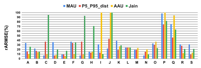
(a) Small (1kb) RPCs. Some error bars exceed 100%.

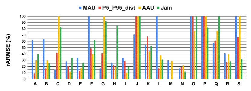
(b) Large (64kb) RPCs. Some error bars exceed 100%.

Figure 13. Prediction error for various AFMs, tail (p99) RPC transmit latency, low QoS.

Fig. 13 shows the prediction error (rARMSE) for low-QoS RPC tail transmit latencies, using the model (linear or queueing-based) that provides the least error, across all 19 fabrics. Using the same $rARMSE\leq 0.15$ accuracy threshold as in described in §6.1, we could not obtain “accurate” prediction models for some fabrics, regardless of which NLM we tried.

One takeaway is that while previous work has often used maximum adjacency utilization as an optimization metric, our results show that this is not always the best choice of NLM. The results also show that the P5-P95-distance metric for imbalance sometimes works well, while using Jain’s index often works quite poorly.

Overall, no single NLM reliably predicts low-QoS RPC tail latencies across all of these fabrics, so training models per-fabric seems essential. In particular, optimizers for systems such as traffic engineering should have fabric-specific goals, rather than relying on a fixed metric.

On the other hand, as shown in Fig. 14, for medium-QoS flows we are much more likely to find accurate models (e.g., for $rARMSE\leq 0.15$) than for low-QoS flows. §D additionally shows that our approach is much more successful at predicting medium-QoS latencies, and median (p50) latencies for low-QoS flows.

Fig. 15 shows that for tail (p1) delivery rates for medium-QoS traffic across all 19 fabrics, we could predict these rates within our 15% threshold – except for Fabrics I, K, and R. (We were unable to extract models for low-QoS delivery rates, because our data included zero-valued p1 (worst-case) samples, which led to division-by-zero errors when calculating rARMSE ($y_{i}=0$ in Eq. 6) We’re trying to understand if RPCAFMs has a bug related to delivery rates on certain connections.)

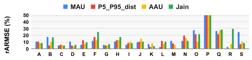
(a) Small RPCs. Some error bars exceed 50%.

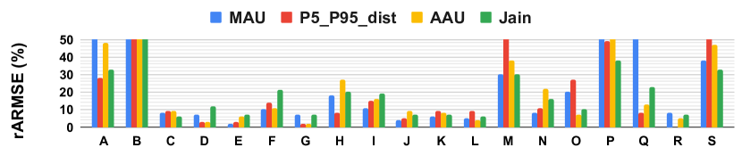
(b) Large RPCs. Some error bars exceed 50%.

Figure 14. Prediction error for tail (p99) transmit latency, medium QoS.

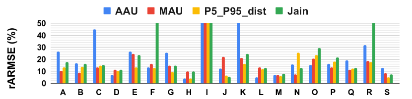
Figure 15. P1 delivery-rate prediction error, medium-QoS. Some error bars exceed 50%.

Fabric AFM A B C D E F G H I J K L M N O P Q R S p50 latency/1kb LQ LQ LQ LQ LQ LQ LQ LQ LQ LQ LQ LQ LQ LQ LQ LQ LQ LQ LQ p99 latency/1kb LQ LQ LQ LQ LQ LQ LQ L LQ X X X X LQ X X X L LQ p50 latency/64kb LQ LQ LQ LQ LQ LQ LQ LQ LQ LQ LQ LQ LQ LQ LQ LQ LQ LQ LQ p99 latency/64kb LQ X LQ LQ X X LQ X LQ X X X X LQ X X X X X

L$=$ predicted by linear model; Q$=$ predicted by queuing-based model; X$=$ predicted by neither.

Table 4. Successful latency predictions (rARMSE$\leq 0.15$) of linear and queueing-based models, low QoS.

7.2. Linear vs. queueing-based models

Table 4 shows the number of tail AFMs predicted, within our 15% threshold, by linear and/or queueing-based models, for fabric-wide low-QoS flows. In every case, linear models make at least as many successful predictions as queuing-based models, and sometimes more. Note that Fig. 10(d) shows that, from week to week, queueing-based models using MAU are sometimes slightly more successful, but Table 4 covers all possible NLMs. Table 6 in §D shows that for medium-QoS flows, linear and queueing-based models were equally successful.

7.3. Coverage

Our approach first finds a knee in the training data, then constructs a model that covers NLM values at and below a knee-based threshold. This raises the question of what fraction of the domain (x-axis buckets) of testing-data samples is covered by such a model, if we do find a high-accuracy model at all.

In most cases, since our networks are often not heavily utilized, we do not detect a knee, and so our models cover 100% of the data. In cases where there is a knee, since the samples are not uniformly distributed across all NLM values, coverage is not a simple function of the threshold.

For fabric-wide predictions for our set of 19 fabrics, we looked at the best models for p50 and p99 transmit latencies for both 1kb and 64kb RPCs, for both low and medium QoS, and in most cases either the coverage was 100% or we found no accurate model. In just five cases (only for p99 latencies), coverage for an accurate model was below 100%, ranging from 83% (fabric $C$, low QoS, 1kB RPCs) to 99% (fabric $N$, low QoS, 64kb RPCs). It is possible that using finer-grained buckets would improve this further.

8. Sensitivity Analysis

Our method has several parameters that can affect either our predictions, or how we measure their success. In this section, we describe the effects of varying some of these parameters.

8.1. Regression Error Threshold

Users can define a threshold rARMSE, based on their operational needs and risk tolerance. A lower threshold reflects a lower tolerance for mis-predictions, but also reduces the number of cases where our method can make successful predictions at a specified target quantile, such as QR95.

Fig. 17 shows the number of latency-based AFMs we could predict, with $rARMSE\leq 0.15$, over the 19-fabric dataset, out of eight possible AFMs (four different RPC sizes, at both p50 and p99), for low-QoS flows. As one would expect, the number decreases as the threshold tightens. Fig. 17 shows the same analysis for medium-QoS flows.

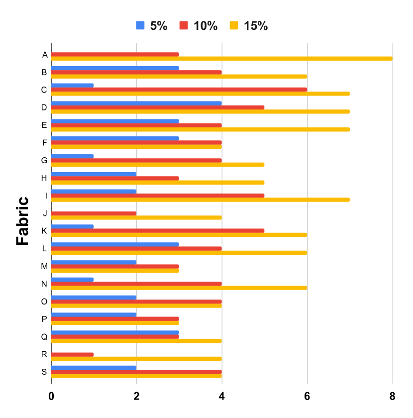
Total number of AFMs analyzed = 8.

Figure 16. # of accurately-predictable AFMs vs. error thresholds, low QoS.

Total number of AFMs analyzed = 8.

Figure 17. # of accurately-predictable AFMs vs. error thresholds, medium QoS.

8.2. Impact of Asymmetric Bias

Our definitions of AMSE and rARMSE include an $\alpha$ parameter. Small values of $\alpha$ penalize underpredictions; large values penalize overpredictions. (We expect most users would prefer to overpredict latency, rather than underpredict.)

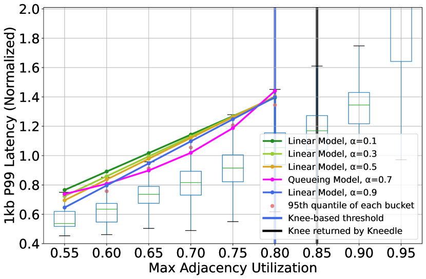
Figure 18. Sensitivity to $\alpha$ for Fabric C

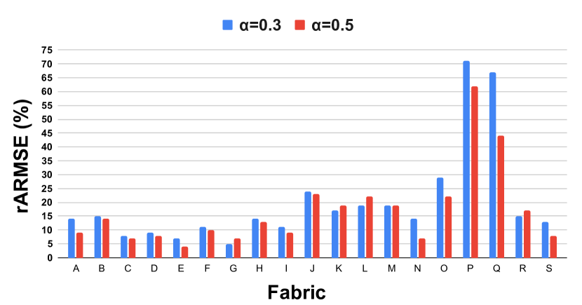
Figure 19. Sensitivity to $\alpha$ across multiple fabrics.

We repeat the single-fabric analysis from Fig. 8, for p99 (tail) latencies, low QoS, NLM $=$MAU, with $\alpha=0.1$, $0.3$, $0.5$ (no bias), $0.7$, and $0.9$. Fig. 19 shows that, as expected, as we decrease $alpha$ we bias towards overprediction (SLO preservation), especially at smaller utilizations. For $alpha=0.7$, we find that the best model is queueing-based. We are not sure why; however, the latencies predicted by the “best” and “worst” of these models are not significantly different.

We looked at fabric-wide rARMSE for all 19 fabrics, with $\alpha=0.3$ and $\alpha=0.5$. Fig. 19 shows (for p99 latencies, low QoS, 1kb RPCs, best-predictor NLMs) that we get similar accuracies even when the user wants to bias in favor of overprediction. I.e., if we create a biased model and then use a biased score, the results are close to what we hoped for, except for fabrics (e.g., $P$ and $Q$) where we get no accurate models.

8.3. Kneedle Curvature Threshold

We augmented Kneedle with curvature threshold $0<\mathcal{C}<1.0$, so that Kneedle only returns knees representing large changes in the AFM. Large $\mathcal{C}$ values reduce false-positive knees, and might make the knee position more stable w.r.t. changes in input data, but risk non-detection of actual knees.

AFM/ Threshold $\mathcal{C}$	0.05	0.1	0.3	0.5	0.7	0.8
1kb p99 Tx. latency	0.85	0.85	0.85	0.85	0.85	X
64kb p99 Tx. latency	0.9	0.9	0.9	0.9	0.9	X

Fabric C, low-QoS RPCs

Table 5. A stable example of knee values vs. curvature thresholds.

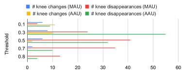
Figure 20. Effect of threshold $\mathcal{C}$ on knee-finding

Our expectations were that the choice of $\mathcal{C}$ would have limited impact on whether and where we detect knees. This is true for some combinations of fabric, QoS, and AFM (see Table 5). In other cases, knees are sensitive to $\mathcal{C}$, and with no fixed pattern. Fig. 20 summarizes results over all 1520 combinations of fabric, QoS, AFM, and threshold (above the minimum of 0.05). It shows that increasing the threshold causes some knee positions to change, and higher thresholds do cause knees to disappear. (We are not sure which of these are “false” knees.) Note that in 82% of the cases (1247/1520), threshold changes had no effect, but for now we need users to experimentally validate their choice of threshold.

9. Discussion

9.1. Takeaways

We summarize several takeaways. These are generalizations to our limited data set, and may not always hold true. Some confirm our intuition or conventional wisdom, some are possibly surprising.

We can construct models that predict AFMs based on individual NLMs, especially at the fabric level and less often at the block level.

No single NLM is universally the best predictor. Our multi-fabric analysis shows that in most cases, the best predictor NLM for an AFM depends on the AFM, QoS, and fabric. Much prior work (e.g.,  (He et al., 2007; Kandula et al., 2005; Wang et al., 2006; Poutievski et al., 2022)) has focused on using MAU or MLU as a predictor; our results suggest that focus is too narrow, as these NLMs are not always the best predictor for AFM performance. Also, because different NLMs predict different knees depending on fabric, it might be safest to use the worst-case AFM-NLM relationship to find the danger zone, rather than hoping for a best-single NLM.

For most cases we studied, a linear relationship fits the data well. Conventional wisdom in our organization was that at low utilizations, RPC latencies would not depend much on NLMs, and if there was a dependency, a queueing-based model would be the best fit. In fact, we found that the best model is almost always linear, even at low utilizations.

Prediction success depends on QoS. This confirms our expectations, as the goal of QoS mechanisms is to differentially protect higher-QoS flows from network conditions.

Short-message latencies are more predictable than long-message latencies. This adds weight to conventional wisdom that congestion-control algorithms tend to respond too slowly to network conditions to affect the sender’s behavior for a short (e.g., 1-packet) message.

Median latencies are easier to predict than tail latencies. This matches our expectations, since generally tail behavior is the result of more complex network behavior.

Prediction accuracy varies from from week to week, even when we re-train models every two weeks. This suggests that, in at least some fabrics, workloads vary enough to make a static model insufficient. However, the nature of a relationship (linear vs. queueing-based) appears to be more stable.

9.2. Limitations of our approach

Our work has several limitations due to constraints of the measurement infrastructure and environment. Not all of the traffic in our network is RPC-based, and not all of the RPC-based traffic is instrumented. We are currently aggregating data into 5-minute buckets, due to RPCAFMs’s limitations, and this hides the effects of short-term bursts. (An alternative would be to collect a burst metric such as the maximum instantaneous queue depth during a measurement period, but our switch instrumentation does not provide this.)

Our results might not be representative for all types of application mixes and fabric types due to several reasons, including the nature of our specific workloads, and the design of our networks and their topologies. In particular, we gathered traces from fabrics which are not heavily used by recently-appearing machine-learning workloads, such as training for large language models.

Appendix A Ethics

This work does not raise any ethical issues. By design, we did not collect any user-identifying data or user data.

Appendix B Details of latency-AFM measurement

Fig. 21 illustrates how RPCAFMs measures RPC “transmit latency.” Note that the time for the last measured byte of a message to transit the network is not included in this measurement.

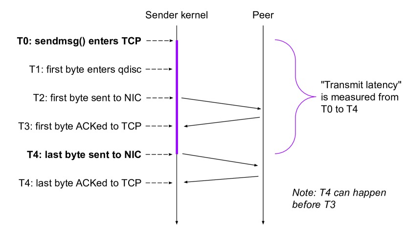
Figure 21. Timing for RPCAFMs transmit latency measurement

Appendix C Effects of quantile-regression thresholds

In §5.2 we described quantile regression, and wrote that we focused on 95th quantiles because at higher percentiles, our datasets were too sparse in some cases to compute low-noise values.) Here we compare how our ability to predict 99th quantile (“QR99”) AFMs compares with our ability to predict QR95 AFMs.

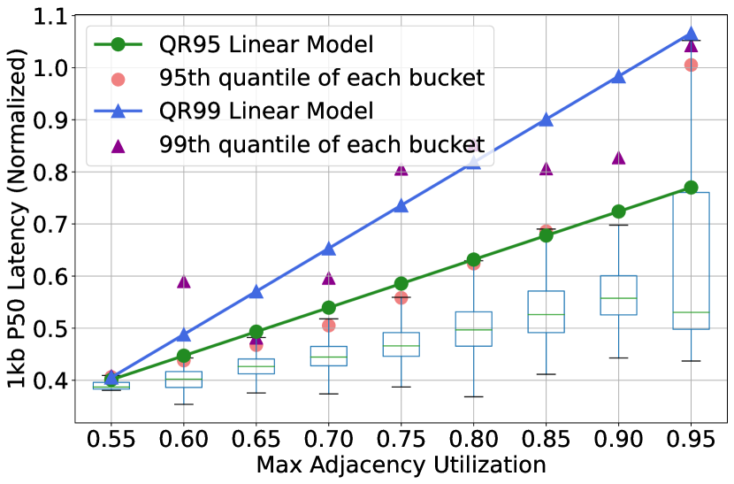
(a) 1kb Median Transmit Latency.

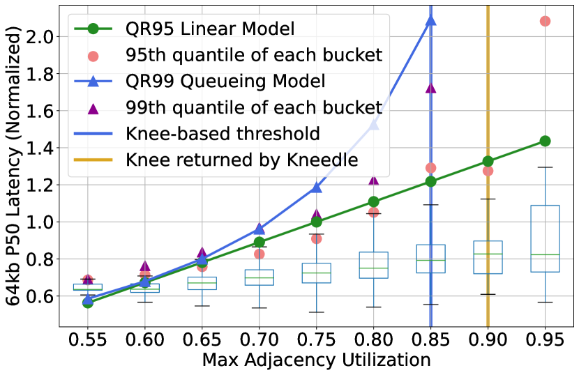
(b) 64kb Median Transmit Latency.

Figure 22. Comparing QR95 and QR99 models for median latency

Fabric C, low QoS, NLM $=$ MAU

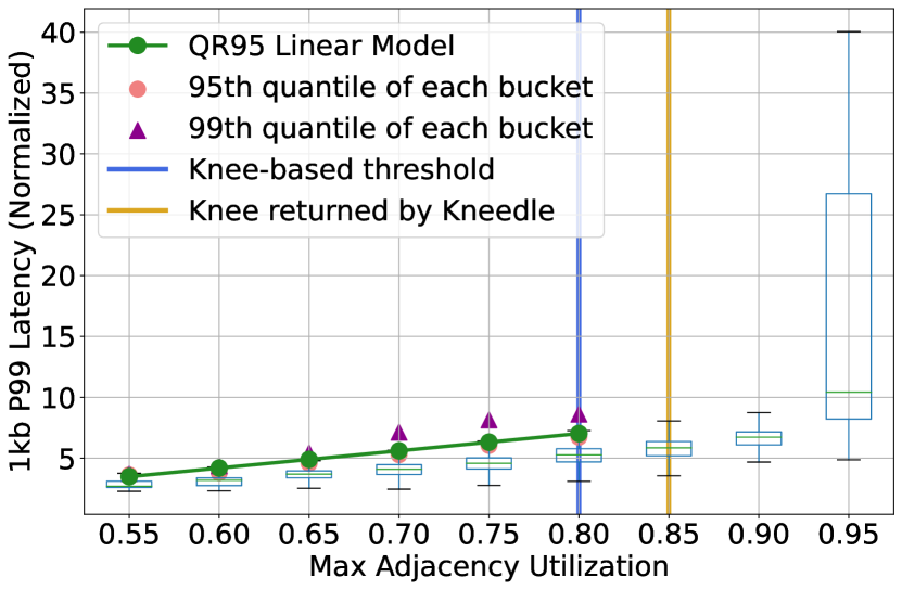
(a) 1kb Tail Transmit Latency.

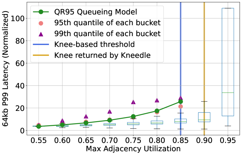
(b) 64kb Tail Transmit Latency.

Figure 23. Comparing QR95 and QR99 models for tail latency

Fabric C, low QoS, NLM $=$ MAU

For a specific example, we looked at fabric-level predictions for Fabric C, as we did in §6. Figures 22(b) and 23 show, respectively, median (p50) and tail (p99) results for low-QoS flows and small-RPC tail-transmit latencies. The figures show both 95th and 99th quantile AFMs for each x-axis bucket, and the QR95 models we obtained in each case. For median transmit latencies (Fig. 22(b)), our method did find high-confidence QR99 models. However, for tail transmit latencies (Fig. 23), we did not find QR99 models; an examination of the “99th quantile” points in that figure suggests that if there is a curve that would fit these points, it is consistent with neither a linear or queueing-based model.

We are unsure whether this failure to produce high-confidence QR99 models is due to intrinsically different behavior for the highest-valued samples in our dataset, or just due to higher noise levels in that subset of the data.

Appendix D Additional inter-block results

To complement Fig. 13 and Fig. 14, which shows per-fabric prediction errors for the p99 (tail) latency of both QoS classes, Figures 24 and 25 present p50 (median) latencies for low-QoS and medium-QoS flows, respectively. Figures 24 and 25 show that p50 latencies are easier to predict successfully than p99 latencies. These results match our expectations. However, even for a given fabric, different (QoS, AFM) combinations can have very different accuracies. For example, fabric $\mathcal{(}J)$ is hard to predict for low-QoS p99 latencies, but apparently much easier to predict for medium-QoS p99 latencies. This could be because low-QoS and medium-QoS flows are drawn from significantly different applications.

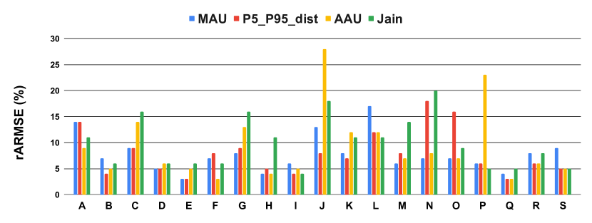
(a) Small RPCs.

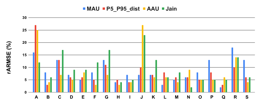
(b) Large RPCs.

Figure 24. Prediction error for various AFMs, median (p50) RPC transmit latency, low QoS.

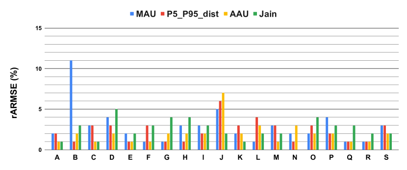
(a) Small RPCs.

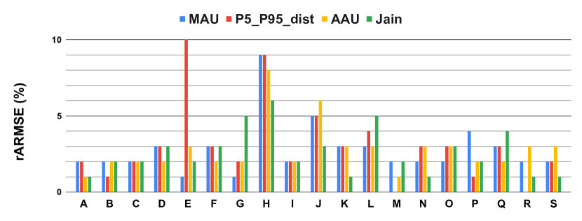
(b) Large RPCs.

Figure 25. Prediction error for various AFMs, median (p50) RPC transmit latency, medium QoS.

Table 4, which showed for low-QoS flows that if we could obtain any “accurate” model for a fabric and AFM, then we could always find an accurate linear model, but in some cases we could not find an accurate queueing-based model. Table 6 shows corresponding results for medium-QoS flows; for these flows, we can find accurate models for a larger fraction of (fabric, AFM) combinations, but here we found accurate queueing-based models in every case where we found an accurate linear model, and vice versa.

Fabric AFM A B C D E F G H I J K L M N O P Q R S p50 latency/1kb LQ LQ LQ LQ LQ LQ LQ LQ LQ LQ LQ LQ LQ LQ LQ LQ LQ LQ LQ p99 latency/1kb LQ LQ LQ LQ LQ LQ LQ LQ LQ LQ LQ LQ LQ LQ LQ X X LQ LQ p50 latency/64kb LQ LQ LQ LQ LQ LQ LQ LQ LQ LQ LQ LQ LQ LQ LQ LQ LQ LQ LQ p99 latency/64kb LQ X LQ LQ LQ LQ LQ LQ LQ LQ LQ LQ X LQ LQ X LQ LQ X

L$=$ predicted by linear model; Q$=$ predicted by queuing-based model; X$=$ predicted by neither.

Table 6. Successful latency predictions (rARMSE$\leq 0.15$) of linear and queueing-based models, medium QoS.

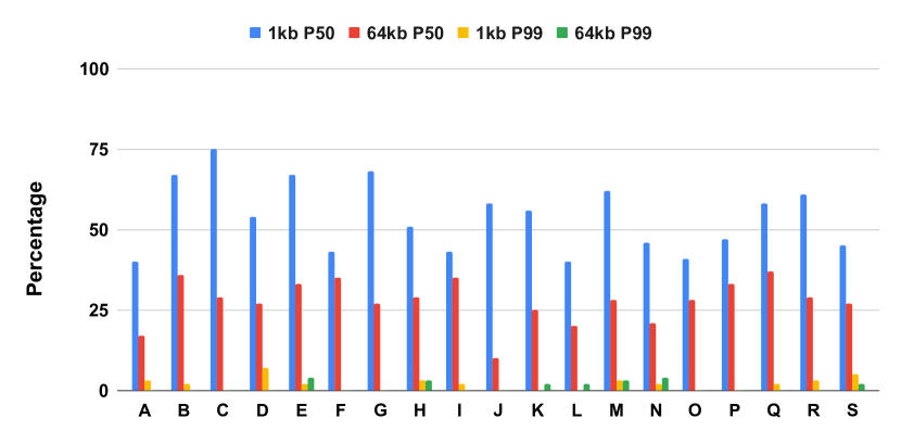
(a) Low QoS.

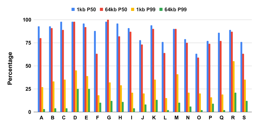
(b) Medium QoS.

Figure 26. Percentage of aggregation blocks, per fabric, with high-accuracy block-local models.

Appendix E Block-local NLM Prediction accuracy

In §6.3, we looked at how well we could predict AFMs for RPCs that stay within aggregation blocks, using NLMs from non-aggregated intra-block links, for Fabric C. Here we extend that analysis to all 19 fabrics.

Figure 26 shows the percentage of aggregation blocks, per fabric, for which we obtained at least one high-accuracy model (using any NLM), broken down by AFM. Fig. 26(a) shows that for low-QoS RPCs, we can predict intra-block median latencies for short RPCs in roughly half of the blocks, and for long RPCs in roughly a quarter of the blocks. Fig. 26(b) shows that for medium-QoS RPCs, which are generally easier to prodict, we can predict intra-block median latencies in well over half the blocks (sometimes in almost all of them), for both RPCs sizes in the figure. However, we cannot predict tail RPC latencies nearly as well, especially for low-QoS RPCs.

References

- (1)
- Agarwal et al. (2022) Saksham Agarwal, Rachit Agarwal, Behnam Montazeri, Masoud Moshref, Khaled Elmeleegy, Luigi Rizzo, Marc Asher de Kruijf, Gautam Kumar, Sylvia Ratnasamy, David Culler, and Amin Vahdat. 2022. Understanding Host Interconnect Congestion. In Proc. HotNets. 198–204.
- Agarwal et al. (2005) Sharad Agarwal, Antonio Nucci, and Supratik Bhattacharyya. 2005. Measuring the shared fate of IGP engineering and interdomain traffic. In 13TH IEEE International Conference on Network Protocols (ICNP’05). IEEE, 10–pp.
- Al-Fares et al. (2008) Mohammad Al-Fares, Alexander Loukissas, and Amin Vahdat. 2008. A Scalable, Commodity Data Center Network Architecture. In Proc. SIGCOMM. 63–74.
- Andreyev (2014) A. Andreyev. 2014. Introducing data center fabric, the next-generation Facebook data center network. https://engineering.fb.com/production-engineering/introducing-data-center-fabric-the-next-generation-facebook-data-center-network/. (2014).
- Applegate et al. (2004) David Applegate, Lee Breslau, and Edith Cohen. 2004. Coping with network failures: Routing strategies for optimal demand oblivious restoration. In Proceedings of the joint international conference on Measurement and modeling of computer systems. 270–281.
- Benson et al. (2010) Theophilus Benson, Aditya Akella, and David A. Maltz. 2010. Network Traffic Characteristics of Data Centers in the Wild. In Proc. IMC. 267–280.
- Callaghan and Rivers (2022) Stpehen Callaghan and JR Rivers. 2022. AWS re:Invent 2022 - Dive deep on AWS networking infrastructure. https://www.youtube.com/watch?v=HJNR_dX8g8c. (2022).
- Cantrill et al. (2004) Bryan M. Cantrill, Michael W. Shapiro, and Adam H. Leventhal. 2004. Dynamic Instrumentation of Production Systems. In Proc. USENIX Annual Technical Conference.
- Cooper (2020) Robert Cooper. 2020. Introduction to Queueing Theory. McMillan.
- Dunning and Ertl (2019) Ted Dunning and Otmar Ertl. 2019. Computing extremely accurate quantiles using t-digests. arXiv preprint arXiv:1902.04023 (2019).
- Fortz and Thorup (2000) B. Fortz and M. Thorup. 2000. Internet traffic engineering by optimizing OSPF weights. In Proc. INFOCOM.
- Gerstel et al. (2014) Ori Gerstel, Clarence Filsfils, Thomas Telkamp, Matthias Gunkel, Martin Horneffer, Victor Lopez, and Arturo Mayoral. 2014. Multi-layer capacity planning for IP-optical networks. IEEE Communications Magazine 52, 1 (2014), 44–51.
- He et al. (2007) Jiayue He, Ma’ayan Bresler, Mung Chiang, and Jennifer Rexford. 2007. Towards Robust Multi-Layer Traffic Engineering: Optimization of Congestion Control and Routing. IEEE Journal on Selected Areas in Communications 25, 5 (2007), 868–880.
- Jain et al. (1984) Rajendra K Jain, Dah-Ming W Chiu, William R Hawe, et al. 1984. A quantitative measure of fairness and discrimination. Eastern Research Laboratory, Digital Equipment Corporation, Hudson, MA 21 (1984).
- Kandula et al. (2005) Srikanth Kandula, Dina Katabi, Bruce Davie, and Anna Charny. 2005. Walking the Tightrope: Responsive yet Stable Traffic Engineering. In Proc. SIGCOMM. 253–264.
- Koenker and Hallock (2001) Roger Koenker and Kevin F Hallock. 2001. Quantile Regression. Journal of economic perspectives 15, 4 (2001), 143–156.
- Kumar et al. (2015) Alok Kumar, Sushant Jain, Uday Naik, Anand Raghuraman, Nikhil Kasinadhuni, Enrique Cauich Zermeno, C. Stephen Gunn, Jing Ai, Björn Carlin, Mihai Amarandei-Stavila, Mathieu Robin, Aspi Siganporia, Stephen Stuart, and Amin Vahdat. 2015. BwE: Flexible, Hierarchical Bandwidth Allocation for WAN Distributed Computing. In Proc. SIGCOMM.
- Kumar et al. (2020) Gautam Kumar, Nandita Dukkipati, Keon Jang, Hassan M. G. Wassel, Xian Wu, Behnam Montazeri, Yaogong Wang, Kevin Springborn, Christopher Alfeld, Michael Ryan, David Wetherall, and Amin Vahdat. 2020. Swift: Delay is Simple and Effective for Congestion Control in the Datacenter. In Proc. SIGCOMM.
- Li et al. (2018) Zhuozhao Li, Haiying Shen, and Ankur Sarker. 2018. A Network-Aware Scheduler in Data-Parallel Clusters for High Performance. In Proc. Symp. on Cluster, Cloud and Grid Computing (CCGRid).
- Mao et al. (2019) Hongzi Mao, Malte Schwarzkopf, Shaileshh Bojja Venkatakrishnan, Zili Meng, and Mohammad Alizadeh. 2019. Learning scheduling algorithms for data processing clusters. In Proceedings of the ACM special interest group on data communication. 270–288.
- Mitra and Ramakrishnan (1999) Debasis Mitra and KG Ramakrishnan. 1999. A case study of multiservice, multipriority traffic engineering design for data networks. In Seamless Interconnection for Universal Services. Global Telecommunications Conference. GLOBECOM’99.(Cat. No. 99CH37042), Vol. 1. IEEE, 1077–1083.
- Namyar et al. (2021) Pooria Namyar, Sucha Supittayapornpong, Mingyang Zhang, Minlan Yu, and Ramesh Govindan. 2021. A Throughput-Centric View of the Performance of Datacenter Topologies. In Proc. SIGCOMM. 349–369.
- Perry et al. (2017) Jonathan Perry, Hari Balakrishnan, and Devavrat Shah. 2017. Flowtune: Flowlet Control for Datacenter Networks. In Proc. NSDI. 421–435.
- Poutievski et al. (2022) Leon Poutievski, Omid Mashayekhi, Joon Ong, Arjun Singh, Mukarram Tariq, Rui Wang, Jianan Zhang, Virginia Beauregard, Patrick Connor, Steve Gribble, Rishi Kapoor, Stephen Kratzer, Nanfang Li, Hong Liu, Karthik Nagaraj, Jason Ornstein, Samir Sawhney, Ryohei Urata, Lorenzo Vicisano, Kevin Yamsura, Shidong Zhang, Junlan Zhou, and Amin Vahdat. 2022. Jupiter Evolving: Transforming Google’s datacenter network via optical circuit switches and software-defined networking. In Proc. SIGCOMM.
- Qureshi et al. (2023) Mubashir Adnan Qureshi, Junhua Yan, Yuchung Cheng, Soheil Hassas Yeganeh, Yousuk Seung, Neal Cardwell, Willem De Bruijn, Van Jacobson, Jasleen Kaur, David Wetherall, and Amin Vahdat. 2023. Fathom: Understanding Datacenter Application Network Performance. In Proc. SIGCOMM. 394–405.
- Satopaa et al. (2011) Ville Satopaa, Jeannie Albrecht, David Irwin, and Barath Raghavan. 2011. Finding a “Kneedle” in a Haystack: Detecting Knee Points in System Behavior. In 2011 31st international conference on distributed computing systems workshops. IEEE, 166–171.
- Valadarsky et al. (2017) Asaf Valadarsky, Michael Schapira, Dafna Shahaf, and Aviv Tamar. 2017. Learning to route. In Proceedings of the 16th ACM workshop on hot topics in networks. 185–191.
- Wang et al. (2006) Hao Wang, Haiyong Xie, Lili Qiu, Yang Richard Yang, Yin Zhang, and Albert Greenberg. 2006. COPE: Traffic Engineering in Dynamic Networks. In Proc. SIGCOMM. 99–110.
- White (2020) Elaheh White. 2020. Statistical Learning for Unimpaired Flow Prediction in Ungauged Basins. Ph.D. Dissertation. University of California, Davis.
- Zhang et al. (2021b) Mingyang Zhang, Jianan Zhang, Rui Wang, Ramesh Govindan, Jeffrey C. Mogul, and Amin Vahdat. 2021b. Gemini: Practical Reconfigurable Datacenter Networks with Topology and Traffic Engineering. CoRR abs/2110.08374 (2021). arXiv:2110.08374 https://arxiv.org/abs/2110.08374
- Zhang et al. (2021a) Qizhen Zhang, Kelvin K. W. Ng, Charles Kazer, Shen Yan, João Sedoc, and Vincent Liu. 2021a. MimicNet: Fast Performance Estimates for Data Center Networks with Machine Learning. In Proc. SIGCOMM. 287–304.
- Zhao et al. (2023a) Kevin Zhao, Prateesh Goyal, Mohammad Alizadeh, and Thomas E. Anderson. 2023a. Scalable Tail Latency Estimation for Data Center Networks. In Proc. NSDI. USENIX Association, Boston, MA, 685–702. https://www.usenix.org/conference/nsdi23/presentation/zhao-kevin
- Zhao et al. (2023b) Shizhen Zhao, Qizhou Zhang, Peirui Cao, Xiao Zhang, Xinbing Wang, and Chenghu Zhou. 2023b. Flattened Clos: Designing High-performance Deadlock-free Expander Data Center Networks Using Graph Contraction. In Proc. NSDI). Boston, MA, 663–683. https://www.usenix.org/conference/nsdi23/presentation/zhao-shizhen
- Zhu et al. (2021) Hang Zhu, Varun Gupta, Satyajeet Singh Ahuja, Yuandong Tian, Ying Zhang, and Xin Jin. 2021. Network planning with deep reinforcement learning. In Proceedings of the 2021 ACM SIGCOMM 2021 Conference. 258–271.