Filling in Missing FX Implied Volatilities with Uncertainties:
Improving VAE-Based Volatility Imputation

Abstract

Missing data is a common problem in finance and often requires methods to fill in the gaps, or in other words, imputation. In this work, we focused on the imputation of missing implied volatilities for FX options. Prior work has used variational autoencoders (VAEs), a neural network-based approach, to solve this problem; however, using stronger classical baselines such as Heston with jumps can significantly outperform their results. We show that simple modifications to the architecture of the VAE lead to significant imputation performance improvements (e.g., in low missingness regimes, nearly cutting the error by half), removing the necessity of using $\beta$-VAEs. Further, we modify the VAE imputation algorithm in order to better handle the uncertainty in data, as well as to obtain accurate uncertainty estimates around imputed values.

1 Introduction

Missing data is a prevalent problem throughout finance and often requires methods to fill in the gaps, or, in other words, imputation. Examples of missing data in finance include reporting inconsistencies (e.g., environmental, social, and governance (ESG) data (e.g., Gopal (2020))) and a lack of pricing data due to illiquidity such as imputing options volatility surfaces (e.g., Heston (1993); Dupire (1994); Brigo and Mercurio (2002); Bergeron et al. (2022); Richert and Buch (2022)) and imputing yield curves (e.g., Vasicek and Fong (1982); Nelson and Siegel (1987); Svensson (1994); Sokol (2022)). In this work, we will specifically focus on the task of imputing missing implied volatilities for FX options.

One classical method to fill in missing values in options surfaces is to fit dynamics models (e.g., Black Scholes, Heston (Heston, 1993), local volatility (Dupire, 1994)) that are consistent with the observed implied volatilities. Another set of methods relies on fitting static models that provably are no-arbitrage (e.g., Mixture of Log Normals (Brigo and Mercurio, 2002), SSVI (Gatheral and Jacquier, 2014)).

While these methods, that are often used in practice, perform well, and are interpretable, given the popularity of neural networks, a natural question is to ask whether or not neural networks can perform better, even if at the cost of interpretability? The value of neural networks is that they are both universal approximators (Cybenko, 1989) and are able to generalize well to unseen data.

One neural network-based method to imputing missing data that has been used recently in the financial literature is variational autoencoders (VAEs) (Bergeron et al., 2022; Richert and Buch, 2022). While only recently explored in the context of finance, using VAEs for imputing data has been explored for many years within the machine learning literature (Rezende et al., 2014; Mattei and Frellsen, 2018a, 2019). However, while the point estimates that come from the VAEs have been tested in terms of imputing FX volatility surfaces, the uncertainty component has not been fully explored.

In this work, we change the commonly used imputation methodology used in VAEs to include uncertainty estimation (distributional imputation), since the value of VAEs in uncertainty modeling. In other words, we focus not only on point estimates, but also on $p(\mathbf{x}_{missing}|\mathbf{x}_{obs})$. Additionally, to improve the imputation of FX volatility surfaces, we:

• incorporate heteroscedastic noise into the decoder/generator (Nazabal et al., 2018), and

• replace the normal multilayer perceptron (MLP) architecture with residual networks (He et al., 2016; Gorishniy et al., 2021).

Finally, we show that, when tested against many classical methods for imputing FX volatility surfaces, VAEs are unable to outperform them without changing the architecture to residual networks.

2 Related Work

One method to impute missing data that has been used recently in the financial literature is variational autoencoders (VAEs). Bergeron et al. (2022) and Sokol (2022) train VAEs directly on market data and then generate point estimates by finding the value in the latent space that best reconstructs the observed data. Richert and Buch (2022) enhances the imputation methodology by using pseudo-Gibbs sampling, originally introduced by Rezende et al. (2014). More details of these approaches are given in Section 6.3.

While only recently explored in the context of finance, using VAEs for imputing data has been explored for many years within the machine learning literature. Rezende et al. (2014) introduced a Gibbs-influenced imputation method; however, this method required that the encoder (introduced later in Section 3.2) is an accurate estimate of the posterior. Mattei and Frellsen (2018a) corrected for this by introducing a Metropolis-within-Gibbs extension. However, this will converge to the right distribution at an impractical convergence rate (Mattei and Frellsen, 2019). Mattei and Frellsen (2019) replaced the Metropolis-within-Gibbs algorithm with importance weighting, an approach that is explained in more detail in Section 6.

3 Background: VAE

The crux of this work is the usage of variational autoencoders (VAEs); in this section, we review the model and discuss some common misconceptions of the model.

Often VAEs are described as “autoencoders with a KL term to regularize the latent encoding”. While this gives a simple description of the loss function, we believe it obfuscates the derivation, usage, and extensions of VAEs. A good description informs users what components can be modified. With the usual description, the method of regularization seems to be a natural way to modify the model; in other words, the usual description positions VAEs as a way to learn a structured latent embedding space. However, in our opinion, a VAE is most useful for imputation when viewed from the generative and statistical angle. To this end, we prefer to describe VAEs as “a deep latent variable model (DLVM) that has been trained using variational inference.” We will define both DLVM (Section 3.1) and variational inference (Section 3.2) in more detail later in this section. We argue that viewing neural networks in this manner allows for a more holistic approach to both fitting the model and imputing data (Section 6).

3.1 Deep Latent Variable Model (DLVM)

What is a deep latent variable model (DLVM)? Statistical models are often easiest to explain via the generative process; thus, a latent variable model can generically be described as:

$$\mathbf{z} \sim p(\mathbf{z})$$

$$\mathbf{x} \sim p(\mathbf{x}|\mathbf{z})$$

where $\mathbf{x}$ is observed and $\mathbf{z}$ is unobserved (latent). A deep latent variable model uses a neural network to parameterize the distributions $p(\mathbf{z})$ and $p(\mathbf{x}|\mathbf{z})$.

The most common way this is achieved is:

$$\begin{split}\mathbf{z}&\sim\mathcal{N}(0,I_{d})\\ \mathbf{x}&\sim\mathcal{N}(\mu_{\theta}(\mathbf{z)},\sigma_{x})\end{split}$$ (3.1)

where $\mathbf{z}\in\mathbb{R}^{d}$ ($d$ will be referred to as latent size or embedding size), $I_{d}$ is an $d\times d$ identity matrix, $\mathbf{x}\in\mathbb{R}^{p}$ ($p$ is the dimensionality of the data, or, in other words, the number of features present in the data), and $\sigma_{x}\in\mathbb{R}$ (we will relax the assumption of $\sigma_{x}$ being a scalar later in Section 5.1). We assume $p(\mathbf{z})$ is a standard Normal distribution and $p(\mathbf{x}|\mathbf{z})$ is a conditional Normal distribution where the mean is parameterized by a neural network $\mu_{\theta}(\mathbf{z)}$ (where $\theta$ denotes the parameters of the function $\mu_{\theta}$) and the standard deviation is a scalar independent of $\mathbf{z}$ ($\sigma_{x}$). The standard deviation either can be fixed throughout training, or can be learned through an unconstrained parameter $s$ where $\sigma_{x}=e^{s}$ or $\sigma_{x}=\log(1+e^{s})=\text{Softplus}(s)$. We will revisit this comment in Section 4 in the context of Beta-VAEs.

In this parameterization, we point out one common mistake when sampling from VAEs: sampling from a VAE requires two sampling steps. Often, when sampling from a VAE, practitioners will sample from $p(\mathbf{z})$ (a Normal distribution) and then use $\mu_{\theta}(\mathbf{z})$ as a sample from the model. However, this is not the true generative process by construction in Equation 3.1. To sample $\mathbf{x}$, we must further sample from another Normal centered at $\mu_{\theta}(\mathbf{z})$ with noise $\sigma$. In Appendix A, using a simple example, we show the negative results of not accounting for this second sampling step.

When fitting distributions to data, the most common method is maximum likelihood estimation (MLE):

$$\operatorname*{argmax}_{\theta}\sum_{i=1}^{N}\log p(\mathbf{x_{i}}|\theta)$$

where $\{\mathbf{x_{i}}\}_{i=1}^{N}$ denotes the data we want to fit our model on. For a latent variable model, the log-likelihood is:

$$\log p(\mathbf{x_{i}}|\theta)=\log\int p(\mathbf{x_{i}}|\mathbf{z},\theta)p(\mathbf{z})d\mathbf{z}$$

This integral is the reason we cannot directly perform gradient descent of the total log-likelihood; we instead use variational inference.

3.2 Variational Inference (VI)

Variational inference approximates the log-likelihood $\log p(\mathbf{x_{i}}|\theta)$ by approximating $p(\mathbf{z}|\mathbf{x_{i}})$ (also known as the posterior). If we were to know $p(\mathbf{z}|\mathbf{x_{i}})$, we could approximate the log integral via:

$$\log p(\mathbf{x_{i}}|\theta)=\mathbb{E}_{\mathbf{z}\sim p(\mathbf{z}|\mathbf{x_{i}})}\left[\log\frac{p(\mathbf{x_{i}}|\mathbf{z},\theta)p(\mathbf{z})}{p(\mathbf{z}|\mathbf{x_{i}})}\right]$$

However, even though we cannot compute $p(\mathbf{z}|\mathbf{x_{i}})$ exactly, we can approximate it with a variational distribution $q(\mathbf{z}|\mathbf{x_{i}})$. Using this approximation, we get the following lower bound:

$$\log p(\mathbf{x_{i}}|\theta) =\log\int p(\mathbf{x_{i}}|\mathbf{z},\theta)p(\mathbf{z})d\mathbf{z}$$ (3.2)

$$=\log\int p(\mathbf{x_{i}}|\mathbf{z},\theta)p(\mathbf{z})\frac{q(\mathbf{z}|\mathbf{x_{i}})}{q(\mathbf{z}|\mathbf{x_{i}})}d\mathbf{z}$$ (3.3)

$$\geq\mathbb{E}_{\mathbf{z}\sim q(\mathbf{z}|\mathbf{x_{i}})}\left[\log\frac{p(\mathbf{x_{i}}|\mathbf{z},\theta)p(\mathbf{z})}{q(\mathbf{z}|\mathbf{x_{i}})}\right]$$ (3.4)

$$=\mathbb{E}_{\mathbf{z}\sim q(\mathbf{z}|\mathbf{x_{i}})}\left[\log p(\mathbf{x_{i}}|\mathbf{z},\theta)\right]+\text{KL}\left(q(\mathbf{z}|\mathbf{x_{i}})\ ||\ p(\mathbf{z})\right)$$ (3.5)

$$=\text{ELBO}(\mathbf{x_{i}}|\theta,q)=-\mathcal{L}_{\text{VAE}}(\mathbf{x_{i}};\theta,\phi)$$ (3.6)

where the last step comes from using Jensen’s inequality. We depict the VAE loss in Figure 1. A useful property of the ELBO (evidence lower bound) is that the gap between it and the true log-likelihood is the KL divergence between the variational distribution and true posterior:

$$\log p(\mathbf{x_{i}}|\theta)-\text{ELBO}(\mathbf{x_{i}}|\theta,q)=\text{KL}\left(q(\mathbf{z}|\mathbf{x_{i}},\theta)\ ||\ p(\mathbf{z}|\mathbf{x_{i}},\theta)\right)$$

Analyzing the $\text{ELBO}(\mathbf{x_{i}}|\theta,q)$, we can see that the description of it as an autoencoder comes from the first term, i.e., $\mathbb{E}_{\mathbf{z}\sim q(\mathbf{z}|\mathbf{x_{i}})}\left[\log p(\mathbf{x_{i}}|\mathbf{z},\theta)\right]$. To make it clearer, plugging in the log-likelihood of a Normal distribution as defined in generative process (Equation 3.1), we get:

$$\mathcal{L}_{\text{VAE}}(\mathbf{x_{i}};\theta,\phi)=\mathbb{E}_{\mathbf{z}\sim q(\mathbf{z}|\mathbf{x_{i}})}\left[\frac{1}{2}\mathinner{\!\left\lVert\frac{\mathbf{\mathbf{x_{i}}}-\mu_{\theta}(\mathbf{z})}{2\sigma_{x}}\right\rVert}^{2}_{2}+\log\left(\sigma_{x}d\sqrt{2\pi}\right)\right]-\text{KL}\left(q(\mathbf{\mathbf{z}}|\mathbf{\mathbf{x_{i}}})||p(\mathbf{\mathbf{z}})\right)$$ (3.7)

The first term is similar to an autoencoder with a mean squared error reconstruction term.

Figure 1: A diagrammatic representation of a vanilla VAE. The two terms on the right side of the diagram are the two terms of the loss function. Interestingly, the KL term is independent of $\theta$ and hence can be calculated before running the decoder (generator) network.

3.3 Reparameterization Trick

To train a VAE, we parametrize $q(\mathbf{z}|\mathbf{x_{i}})$ with a neural network, often as:

$$\mathbf{h} =f_{\phi}(\mathbf{x_{i}})$$ (3.8)

$$\mathbf{z} \sim\mathcal{N}(\mu_{\phi}(\mathbf{h}),\sigma_{\phi}(\mathbf{h}))$$ (3.9)

where $f_{\phi}$ is a neural network and often $\mu_{\phi}$ and $\sigma_{\phi}$ are simple linear transformations (but could also be neural networks).

Since VAEs are parameterized by neural networks, we train them using gradient descent. Computing the gradient of the loss function with respect to $\theta$ is straightforward using automatic differentiation (we would only need to compute $\frac{\partial\log p_{\theta}(\mathbf{x_{i}}|\mathbf{z})}{\partial\theta}$ since the KL term is independent of $\theta$). However, computing the gradient with respect to $\phi$ is non-trivial since:

$$\frac{\partial\ \text{ELBO}(\mathbf{x_{i}}|\theta,q_{\phi})}{\partial\phi}=\frac{\partial\ \text{ELBO}(\mathbf{x_{i}}|\theta,q_{\phi})}{\partial\mathbf{z}}\left[\frac{\partial\mathbf{z}}{\partial\mu_{\mathbf{z}|\mathbf{x}}}\frac{\partial\mu_{\mathbf{z}|\mathbf{x}}}{\partial\phi}+\frac{\partial\mathbf{z}}{\partial\sigma_{\mathbf{z}|\mathbf{x}}}\frac{\partial\sigma_{\mathbf{z}|\mathbf{x}}}{\partial\phi}\right]$$

where we used chain rule and the notation from Figure 1.$\frac{\partial\mu_{\mathbf{z}|\mathbf{x}}}{\partial\phi}$ and $\frac{\partial\sigma_{\mathbf{z}|\mathbf{x}}}{\partial\phi}$ are trivial to differentiate using automatic differentiation, but how do we differentiate $\frac{\partial\mathbf{z}}{\partial\mu_{\mathbf{z}|\mathbf{x}}}$ and $\frac{\partial\mathbf{z}}{\partial\sigma_{\mathbf{z}|\mathbf{x}}}$? The difficulty arises from the fact that $\mathbf{z}$ is a random function of $\mu_{\mathbf{z}|\mathbf{x}}$ and $\sigma_{\mathbf{z}|\mathbf{x}}$. To ensure the sampling is differentiable, we use the reparameterization trick: we can rewrite sampling from $\mathbf{z}\sim\mathcal{N}(\mu_{\phi}(\mathbf{h}),\sigma_{\phi}(\mathbf{h}))$ (where the parameters are a part of the random function) as:

$$\mathbf{\epsilon} \sim\mathcal{N}(0,1)$$ (3.10)

$$\mathbf{z} =\mu_{\phi}(\mathbf{h})+\sigma_{\phi}(\mathbf{h})\cdot\mathbf{\epsilon}$$ (3.11)

The distribution is still the same, but now the parameters are not being directly used in the randomization. Thus, $\frac{\partial\mathbf{z}}{\partial\mu_{\mathbf{z}|\mathbf{x}}}=1$ and $\frac{\partial\mathbf{z}}{\partial\sigma_{\mathbf{z}|\mathbf{x}}}=\mathbf{\epsilon}$. The reparameterization trick can be generalized to any continuous distribution for which we know the inverse CDF function ($\mathcal{F}^{-1}$):

$$\mathbf{\epsilon} \sim\mathcal{U}(0,1)$$

$$\mathbf{z} =\mathcal{F}^{-1}(\mathbf{\epsilon})$$

where $\mathcal{U}$ is a uniform distribution.

3.4 Handling Missing Data

Since the overall goal of our paper is to use VAEs for filling in missing data, we expect that our training data will also contain missing values. To handle missing data in probabilistic modeling, we must marginalize out (integrate out) the missing variables.

For example, say our data is $\mathbf{x}=\mathbf{x}_{\text{obs}}\ ||\ \mathbf{x}_{\text{miss}}$ ($\mathbf{x}$ is the concatenation of a vector of observed data and a vector of missing data). Assume we are modeling the data using a deep latent variable model and that $\mathbf{x_{i}}\mathop{\underline{\raisebox{0.0pt}[0.0pt][1.0pt]{$\;||\;$}}}\mathbf{x_{j}}|\mathbf{z}$ (each variable is conditionally independent given $\mathbf{z}$). We then get:

$$\log p(\mathbf{x}_{\text{obs}}|\theta) =\log\int p(\mathbf{x}_{\text{obs}},\mathbf{x}_{\text{miss}}|\mathbf{z},\theta)p(\mathbf{z})\ d\mathbf{x}_{\text{miss}}\ d\mathbf{z}$$ (3.12)

$$=\log\int p(\mathbf{x}_{\text{obs}}|\mathbf{z},\theta)\ p(\mathbf{x}_{\text{miss}}|\mathbf{z},\theta)\ p(\mathbf{z})\frac{q(\mathbf{z}|\mathbf{x}_{\text{obs}})}{q(\mathbf{z}|\mathbf{x}_{\text{obs}})}\ d\mathbf{x}_{\text{miss}}\ d\mathbf{z}$$ (3.13)

$$\geq\mathbb{E}_{\mathbf{z}\sim q(\mathbf{z}|\mathbf{x}_{\text{obs}})}\left[\log\int\frac{p(\mathbf{x}_{\text{obs}}|\mathbf{z},\theta)\ p(\mathbf{x}_{\text{miss}}|\mathbf{z},\theta)\ p(\mathbf{z})}{q(\mathbf{z}|\mathbf{x}_{\text{obs}})}\ d\mathbf{x}_{\text{miss}}\right]$$ (3.14)

$$=\mathbb{E}_{\mathbf{z}\sim q(\mathbf{z}|\mathbf{x}_{\text{obs}})}\left[\log\frac{p(\mathbf{x}_{\text{obs}}|\mathbf{z},\theta)\ p(\mathbf{z})}{q(\mathbf{z}|\mathbf{x}_{\text{obs}})}\right]$$ (3.15)

Practically, in terms of implementation, the loss function with missing data is as simple as masking out the “reconstruction” terms for the missing values. While the change might seem trivial of an extension, the derivation above gives a simple but rigorous justification of the implementation.

3.5 Reviewing the Definition of VAE

Returning back to the definition we introduced earlier for VAEs, we can see that VAEs are based on two design decisions: 1) Using deep latent variable models and 2) Training this model with variational inference. Variational inference can be used to train other models such as a Gaussian Mixture Models or Latent Dirichlet Allocation (Blei et al., 2003) (neither of which relies on neural networks). Additionally, we could train DLVMs using other methods besides variational inference such as MCMC (Markov chain Monte Carlo), or even adversarial training. The view of a VAE as a regularized autoencoder is an overly specific description of the loss function, and we suggest that the fact that the loss function looks like a regularized autoencoder is more an outcome of the optimization process (using variational inference) and arguably is a coincidence (Equation 3.7). Finally, by centering our definition on a distributional definition instead of an autoencoder definition, we believe that the uncertainty-based component is better highlighted.

Realizing that there are many distributional components in a VAE, namely $q(\mathbf{z}|\mathbf{x})$, $p(\mathbf{z})$, and $p(\mathbf{x}|\mathbf{z})$, we could replace each distribution with something besides a Normal distribution. For example, we could use a more expressive family of distributions such as normalizing flows for $q(\mathbf{z}|\mathbf{x})$ (Rezende and Mohamed, 2015). Further, we could use a mixture distribution for $p(\mathbf{z})$ as was done by Jiang et al. (2017) to allow the VAE to learn to cluster the data. We could use a multinomial distribution for $p(\mathbf{x}|\mathbf{z})$ if our data is categorical, or a Poisson if it is counts data (Nazabal et al., 2018), and even for continuous data, we could use a heavier tailed distribution such as a Logistic distribution (e.g., (Vahdat and Kautz, 2020)). Arguably, from the autoencoder viewpoint, these changes are not as obvious to make as they are from the perspective of distributional modeling.

4 Why We Do Not Use Beta-VAE

From the perspective of a VAE as a regularized autoencoder, a natural extension would be to add an additional hyperparameter to control the amount of regularization:

$$\mathcal{L}_{\beta\mathchar 45\relax\text{VAE}}(\mathbf{x};\beta,\theta,\phi,)=\mathbb{E}_{\mathbf{z}\sim q(\mathbf{z}|\mathbf{x})}\left[\mathinner{\!\left\lVert\mathbf{x}-\mu_{\theta}(\mathbf{z})\right\rVert}^{2}\right]-\beta\ \text{KL}\left(q(\mathbf{z}|\mathbf{x_{i}})||p(\mathbf{z})\right)$$ (4.1)

Using this loss function is referred to as a Beta-VAE (Higgins et al., 2017), or $\beta$-VAE. While this is natural in the autoencoder perspective and has been used many times in the financial literature for imputation, what is the interpretation in the distributional perspective?

We repeat the VAE loss for the specific generative process (Equation 3.1) here:

$$\mathcal{L}_{\sigma\mathchar 45\relax\text{VAE}}(x_{i};\sigma_{x}),\theta,\phi)=\mathbb{E}_{z\sim q(z|x_{i})}\left[\frac{1}{2}\mathinner{\!\left\lVert\frac{\mathbf{x_{i}}-\mu_{\theta}(\mathbf{z})}{\sigma_{x}}\right\rVert}^{2}_{2}+\log\left(\sigma_{x}d\sqrt{2\pi}\right)\right]-\text{KL}\left(q(\mathbf{z}|\mathbf{x_{i}})||p(\mathbf{z})\right)$$ (4.2)

By comparing and contrasting these two loss functions, we will be able to better understand why $\beta$-VAE has been useful, and, more importantly, how we generalize it to be more effective in practice.

First, let’s assume that $\sigma_{x}$ is fixed and not a learnable parameter. To compare $\mathcal{L}_{\beta-\text{VAE}}$ and $\mathcal{L}_{\sigma-\text{VAE}}$, we remind ourselves that it isn’t crucial to compare the value of the two loss functions, but instead to compare the minima of the two:

$$\operatorname*{argmin}_{\theta,\phi}\mathcal{L}_{\sigma\mathchar 45\relax\text{VAE}}(\mathbf{x_{i}};\sigma_{x},\theta,\phi) =\operatorname*{argmin}_{\theta,\phi}\mathbb{E}_{z\sim q(z|x_{i})}\left[\frac{1}{2}\mathinner{\!\left\lVert\frac{\mathbf{x_{i}}-\mu_{\theta}(\mathbf{z})}{\sigma_{x}}\right\rVert}^{2}_{2}+\log\left(\sigma_{x}d\sqrt{2\pi}\right)\right]-\text{KL}\left(q(\mathbf{z}|\mathbf{x_{i}})||p(\mathbf{z})\right)$$ (4.3)

$$=\operatorname*{argmin}_{\theta,\phi}\mathbb{E}_{z\sim q(z|x_{i})}\left[\frac{1}{2\sigma_{x}^{2}}\mathinner{\!\left\lVert\mathbf{x_{i}}-\mu_{\theta}(\mathbf{z})\right\rVert}^{2}\right]-\text{KL}\left(q(\mathbf{z}|\mathbf{x_{i}})||p(\mathbf{z})\right)$$ (4.4)

$$=\operatorname*{argmin}_{\theta,\phi}\mathbb{E}_{z\sim q(z|x_{i})}\left[\mathinner{\!\left\lVert\mathbf{x_{i}}-\mu_{\theta}(\mathbf{z})\right\rVert}^{2}\right]-2\sigma_{x}^{2}\text{KL}\left(q(\mathbf{z}|\mathbf{x_{i}})||p(\mathbf{z})\right)$$ (4.5)

$$=\operatorname*{argmin}_{\theta,\phi}\mathcal{L}_{\beta\mathchar 45\relax\text{VAE}}(\mathbf{x_{i}};2\sigma_{x}^{2},\theta,\phi)$$ (4.6)

In other words, optimizing a $\sigma\mathchar 45\relax\text{VAE}$ with a fixed $\sigma_{x}$ is equivalent to optimizing a $\beta$-VAE where $\beta=2\sigma_{x}^{2}$. Thus, from the distributional perspective, $\beta$ simply controls the variance of the Normal distribution on the decoder side.

While this might seem simply to be an interesting mathematical connection, there is one major reason to use $\sigma\mathchar 45\relax\text{VAE}$ instead of $\beta$-VAE: we can learn $\sigma$ instead of tune it. If $\sigma_{x}$ is not fixed, there is an additional term that $\beta$-VAE does not have: $\log\left(\sigma_{x}d\sqrt{2\pi}\right)$. This “correction term” allows us to optimize $\sigma_{x}$ instead of treating it as a hyperparameter that must be tuned.

We run a simple experiment to highlight this point. We train four models:

• Model 1: $\beta$-VAE with $\beta=1$

• Model 2: $\beta$-VAE with $\beta=0.1$

• Model 3: $\beta$-VAE with learnable $\beta$

• Model 4: $\sigma$-VAE with learnable $\sigma$

We show the (synthetic) data we trained our VAEs on in Figure 3. To ensure no underfitting, we trained all models for 100K steps. Additional details on architecture and training methodology can be found in Appendix B.2.

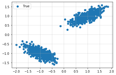
Figure 2: Mixture of two Gaussians.

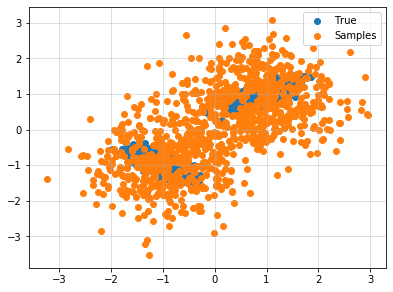
(a) $\beta=1$

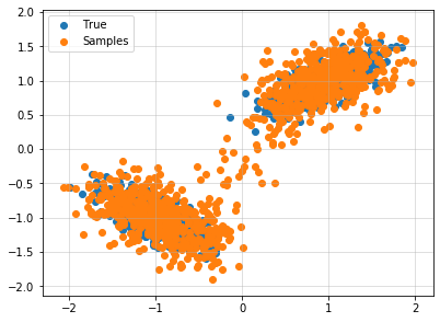
(b) $\beta=0.1$

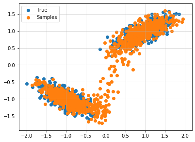
(c) Learnable $\beta$

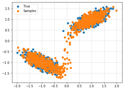
(d) $\sigma$-VAE

Figure 3: Comparison of generations by different VAEs.

To create the generations for the $\beta$-VAE that we see in Figure 3, we modify the variance $\sigma^{2}_{x}$ to be $\sigma_{x}^{2}=\frac{\beta}{2}$. We can see that the quality of generations with $\beta=1$ is low as a result of not training the output variance ($\sigma_{x}$). We see that lowering $\beta$ helps improve the generations. However, for the learnable $\beta$, the final $\beta$ was $1e{-4}$, which is to be expected as it is optimal to remove the KL-term when minimizing the $\beta$-VAE loss. From a practical standpoint, this is suboptimal as the intention of $\beta$ is to “regularize” the latent space. On the other hand, for the $\sigma$-VAE, the quality of the generations is good (and will be improved in a later section (Section 5.2)) and has a final learned $\sigma_{x}=0.127$. Thus, while good generations might be attainable by a $\beta$-VAE, finding the optimal $\beta$ requires training multiple models, and tuning $\beta$ whereas $\sigma$-VAE requires training only once. We show in the next section (Section 5.1) that heteroscedastic noise is easy to account for in a $\sigma$-VAE, but is impractical for $\beta$-VAE due to the massive increase in hyperparameters.

5 Improving Training Methodology of VAEs

5.1 Heteroscedasticity

Having realized that we can simply use $\sigma\mathchar 45\relax VAE$ to remove the need to hyperparameter tune $\beta$ in $\beta\mathchar 45\relax VAE$ (Section 4), we can easily extend the VAE to allow for each feature to have a different amount of noise. We can easily replace the scalar $\sigma_{x}$ with a vector $\mathbf{\sigma_{x}}\in\mathbb{R}^{p}$ and optimize the amount of noise for each feature jointly with all the other parameters ($\theta$ and $\phi$):

$$\mathcal{L}_{\mathbf{\vec{\sigma}}\mathchar 45\relax\text{VAE}}(\mathbf{x_{i}};\sigma_{x},\theta,\phi)=\mathbb{E}_{z\sim q(z|x_{i})}\left[\frac{1}{2}\mathinner{\!\left\lVert\frac{\mathbf{x_{i}}-\mu_{\theta}(\mathbf{z})}{\mathbf{\sigma_{x}}}\right\rVert}^{2}_{2}+\sum_{i=1}^{p}\log\left(\sqrt{2\pi}\sigma_{x,i}\right)\right]-\text{KL}\left(q(\mathbf{z}|\mathbf{x_{i}})||p(\mathbf{z})\right)$$ (5.1)

If this were a $\beta$-VAE, this would introduce a hyperparameter per input dimension (feature), i.e., $p$ hyperparameters; here, with the distributional perspective of VAEs, we introduce no new hyperparameters.

Further, we can make $\mathbf{\sigma_{x}}$ a function of $z$:

$$\mathcal{L}_{{{\Sigma}}\mathchar 45\relax\text{VAE}}(\mathbf{x_{i}},\theta,\phi)=\mathbb{E}_{z\sim q(z|x_{i})}\left[\frac{1}{2}\mathinner{\!\left\lVert\frac{(\mathbf{x_{i}}-\mu_{\theta}(\mathbf{z}))}{\sigma_{\theta}(z)}\right\rVert}^{2}_{2}+\sum_{i=1}^{p}\log\left(\sqrt{2\pi}(\sigma_{\theta}(z))_{i}\right)\right]-\text{KL}\left(q(\mathbf{z}|\mathbf{x_{i}})||p(\mathbf{z})\right)$$ (5.2)

To test the effect of this, similar to Section 4, we generate a mixture of two Gaussians; however, we set the variances of the two modes to be different (Figure 5). In Figure 5, we compare training with a single $\sigma_{x}$ versus a function $\mathbf{\sigma_{\theta}}$. While it might not be clear from the generations the difference in performance, the loss curve shows clearly the $\Sigma$-VAE outperforming. Additional details on architecture and training methodology can be found in Appendix B.3.

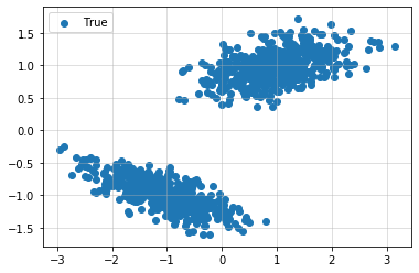
Figure 4: Mixture of two Gaussians.

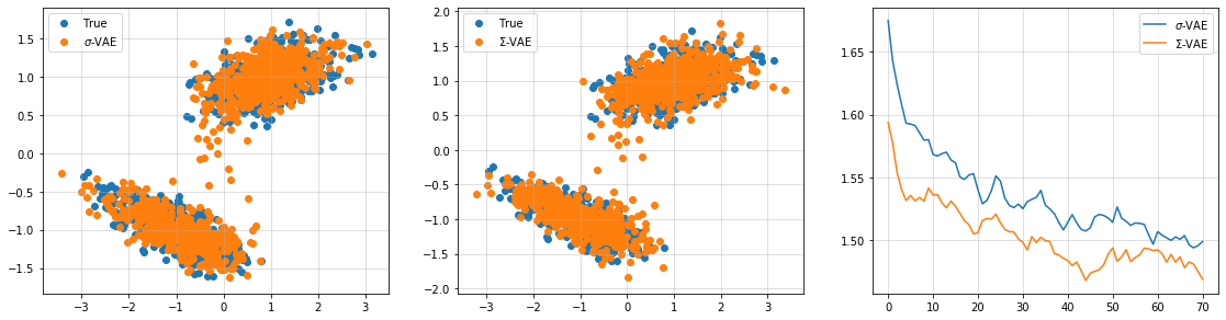
(a) $\sigma$-VAE

(b) $\Sigma$-VAE

(c) Loss

Figure 5: Comparison of generations and loss curves of two different VAEs.

5.2 Importance Weighted Autoencoder (IWAE)

A simple trick to help close the gap in the lower bound is to use importance weighted autoencoders:

$$\log p(\mathbf{x_{i}}|\theta)\geq\mathbb{E}_{\mathbf{z_{1}},\dots,\mathbf{z_{k}}\sim q(\mathbf{z}|\mathbf{x_{i}})}\left[\log\sum_{j}\frac{1}{k}\frac{p(\mathbf{x_{i}}|\mathbf{z_{j}},\theta)p(\mathbf{z_{j}})}{q(\mathbf{z_{j}}|\mathbf{x_{i}})}\right]=-\mathcal{L}_{\text{IWAE},k}$$ (5.3)

As shown by Burda et al. (2015), with some abuse of notation, we have

$$\log p(\mathbf{x_{i}}|\theta) =-\mathcal{L}_{\text{IWAE},\infty}$$ (5.4)

$$\geq\mathcal{L}_{\text{IWAE},k+1}\geq-\mathcal{L}_{\text{IWAE},k}$$ (5.5)

$$\geq-\mathcal{L}_{\text{IWAE},1}=-\mathcal{L}_{\text{VAE}}$$ (5.6)

which implies using a larger $k$ reduces the bias of the estimator.

Note:

$$\log p(\mathbf{x_{i}}|\theta) \geq-\mathcal{L}_{\text{VAE}}$$ (5.7)

$$=\mathbb{E}_{\mathbf{z}\sim q(\mathbf{z}|\mathbf{x_{i}})}\left[\log\frac{p(\mathbf{x_{i}}|\mathbf{z},\theta)p(\mathbf{z})}{q(\mathbf{z}|\mathbf{x_{i}})}\right]$$ (5.8)

$$=\mathbb{E}_{\mathbf{z_{1}},\dots,\mathbf{z_{m}}\sim q(\mathbf{z}|\mathbf{x_{i}})}\left[\sum_{j}\frac{1}{m}\log\frac{p(\mathbf{x_{i}}|\mathbf{z_{j}},\theta)p(\mathbf{z_{j}})}{q(\mathbf{z_{j}}|\mathbf{x_{i}})}\right]$$ (5.9)

where, as opposed to the IWAE loss (Equation 5.3), sampling $m$ times from $q(\mathbf{z}|\mathbf{x_{i}})$ does not reduce the bias but instead reduces the variance of the estimator of the VAE loss.

Using the synthetic data shown in Figure 3, we show in Figure 6 the effect of using importance weighted autoencoders on bimodal data. Additional details on architecture and training methodology can be found in Appendix B.2. While the VAE struggles to fully capture the bimodality of the data, the IWAE is better able to handle this, leading to higher quality generations.

(a) $\sigma$-VAE

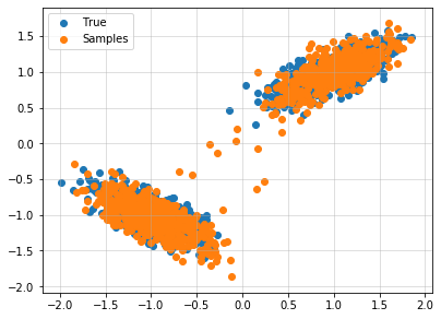
(b) $\sigma$-IWAE

Figure 6: Comparison of generations by VAEs vs. IWAEs

Note, while our experiments in Section 7.2.2 show that training IWAEs does not help for FX volatility imputation, we do still utilize the IWAE loss for evaluation since we want an accurate estimate of $\log p(\mathbf{x_{i}}|\theta)$ for model comparison.

5.3 Residual Networks

An additional adjustment we make, and the most important according to our experiments (Section 7.2.1), is changing the architecture to residual networks. Normally, for tabular data, a feed forward network is used. However, with the continued success of residual networks in the context of convolutions (He et al., 2016; Zagoruyko and Komodakis, 2016), transformers (Vaswani et al., 2017), and normalizing flows (i.e., residual flows, Chen et al. (2019)), we use residual networks as the backbone of our model, similar to the MLP blocks used in transformers (Figure 8). Preliminary experiments showed better convergence when utilizing Swish ($=x*\text{Sigmoid}(x)$) (Ramachandran et al., 2018) over GELU and ReLU. We incorporate dropout after the activation layer and the second linear layer in the residual branch, similar to Transformers. A similar architecture has been previously introduced by Gorishniy et al. (2021). However, Gorishniy et al. (2021) used Batch Normalization (Ioffe and Szegedy, 2015) instead of Layer Normalization (Ba et al., 2016) and used ReLU instead of Swish.

Figure 7: Diagram showing a traditional MLP block. $\sigma$ denotes a non-linear activation.

Figure 8: Diagram showing a VAE comprised of traditional MLP blocks.

Figure 9: Diagram showing a residual block. In our model, we use square matrices for $W_{1}$ and $W_{2}$, and we use Swish for the activation $\sigma$.

Figure 10: Diagram showing a VAE comprised of residual blocks. We use “LN” to denote Layer Normalization.

To make the differences clearer, we show the conventional approach to MLPs in Figure 8 and Figure 8 and show the approach using residual networks in in Figure 10 and Figure 10. Mathematical notation describing the VAE comprised of residual networks can be found in Appendix B.1.

To compare the two architectures, we fit them to a mixture of eight Gaussians (Figure 12). In Figure 12, we see that the residual network is able to easily learn this distribution while the normal feedforward struggles. We see this both from the quality of samples where the residual network is better able to capture the multimodality (Figure 12 and Figure 12) as well as in the gap in loss curves (Figure 12). Additional details on architecture and training methodology can be found in Appendix B.4.

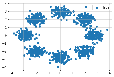
Figure 11: Mixture of eight Gaussians.

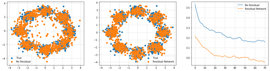
(a) MLP VAE

(b) Residual VAE

(c) Loss

Figure 12: Comparison of generations and loss curves with and without using residual blocks.

5.3.1 Intuition of Efficacy of Residual Networks

To build an intuition on the residual architecture, looking at Figure 10, we can see, from a gradient perspective, there is “direct path” from the reconstruction loss to $\mu_{\mathbf{z}|\mathbf{x}}$ as opposed to Figure 8. We analyze the impact of this architectural detail by analyzing:

$$\mathinner{\!\left\lVert\frac{1}{N}\sum_{i=1}^{N}\frac{\partial\mathbb{E}_{\mathbf{z}\sim q(\mathbf{z}|\mathbf{x_{i}})}\left[\log p(\mathbf{x_{i}}|\mathbf{z})\right]}{\partial\mu_{\mathbf{z}|\mathbf{x}}}\right\rVert}_{2}$$

which we will refer to as the gradient norm of the reconstruction term, and:

$$\qquad\mathinner{\!\left\lVert\frac{1}{N}\sum_{i=1}^{N}\frac{\partial\text{KL}\left(q(\mathbf{z}|\mathbf{x_{i}})\ ||\ p(\mathbf{z})\right)}{\partial\mu_{\mathbf{z}|\mathbf{x}}}\right\rVert}_{2}$$

which we will refer to as the gradient norm of the KL term. In Figure 13, we plot these two quantities (averaged across 500 batches) as a function of training steps for a VAE with and without residual connections. We find that:

1. The gradient norm of the reconstruction term starts small for VAEs without residual connections

2. The gradient norm of the reconstruction term on average is larger with residual connections than without. Further, the gradient norm of the KL term is comparable.

The second observation is interesting since the original intention of $\beta$-VAE was to reduce the regularization from the KL term which is equivalent to reducing the gradient norm of the KL term. By using residual connections, we get this behavior without having to modify the loss function, retaining the probabilistic interpretation of VAEs.

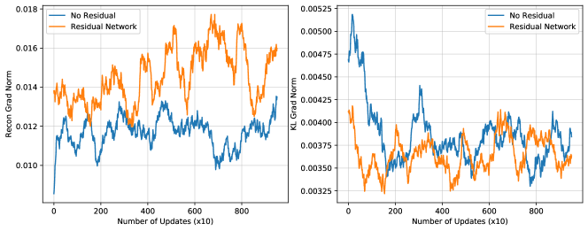
Figure 13: Comparison of gradient norm of reconstruction term and KL term for VAEs with and without residual connections.

Further, if we were to remove all the residual paths (the paths from the Layer Norm to the layer before the elementwise addition), we would get a linear model, and a linear VAE has connections to probabilistic PCA (Ghojogh et al., 2021) and factor analysis. Given the efficacy of PCA in finance, we intuit this connection to be a source of the performance we see in Section 7.2.1.

6 Distributional Imputation

Since we are focused on uncertainties and probabilities, we view imputation as querying $p(\mathbf{x_{m}}|\mathbf{x_{o}})$ where $\mathbf{x_{m}}$ and $\mathbf{x_{o}}$ is a partitioning of $\mathbf{x}$ where $\mathbf{x_{o}}$ is the subset of features observed and $\mathbf{x_{m}}$ is the subset of features missing. We focus on $p(\mathbf{x_{m}}|\mathbf{x_{o}})$ generically as we can view point estimates as the mean $\mathbb{E}\left[p(\mathbf{x_{m}}|\mathbf{x_{o}})\right]$ and uncertainty estimates as the variance $\mathbb{V}\left[p(\mathbf{x_{m}}|\mathbf{x_{o}})\right]$.

6.1 Algorithm and Derivation

The question then is, how do we sample from $p(\mathbf{x_{m}}|\mathbf{x_{o}})$? To begin, we first use the law of total probability:

$$p(\mathbf{x_{m}}|\mathbf{x_{o}})=\int p(\mathbf{x_{m}}|\mathbf{x_{o}},\mathbf{z})\ p(\mathbf{z}|\mathbf{x_{o}})\ d\mathbf{z}$$

Algorithmically, we can read the integral as:

1. Sample $\mathbf{z}$ from $p(\mathbf{z}|\mathbf{x_{o}})$

2. Sample $\mathbf{x_{m}}$ from $p(\mathbf{x_{m}}|\mathbf{x_{o}},\mathbf{z})$

Note, $p(\mathbf{x_{m}}|\mathbf{x_{o}},\mathbf{z})=p(\mathbf{x_{m}}|\mathbf{z})$ by construction of our VAE since, conditional on $\mathbf{z}$, $\mathbf{x}$ is distributed as $p$-independent Gaussians.

To sample from $p(\mathbf{z}|\mathbf{x_{o}})$, we see using Bayes rule that $p(\mathbf{z}|\mathbf{x_{o}})\propto p(\mathbf{x_{o}}|\mathbf{z})p(\mathbf{z})$, or algorithmically:

1. Sample $\mathbf{z_{i}}$ from $p(\mathbf{z})$ $n$ times

2. Reweigh each $\mathbf{z_{i}}$ by $\frac{p(\mathbf{x_{o}}|\mathbf{z_{i}})}{\sum_{j}p(\mathbf{x_{o}}|\mathbf{z_{j}})}$

However, since $p(\mathbf{z}|\mathbf{x_{o}})$ is the posterior and the encoder $q(\mathbf{z}|\mathbf{x_{o}})$ is meant to be an approximation of the posterior, we can rewrite:

$$p(\mathbf{z}|\mathbf{x_{o}})\propto p(\mathbf{x_{o}}|\mathbf{z})p(\mathbf{z})\frac{q(\mathbf{z}|\mathbf{x_{o}})}{q(\mathbf{z}|\mathbf{x_{o}})}$$

1. Sample $z_{i}$ from $q(\mathbf{z}|\mathbf{x_{o}})$ $n$ times

2. Reweigh each $z_{i}$ by $\frac{p(\mathbf{x_{o}}|\mathbf{z_{i}})p(\mathbf{z_{i}})}{q(\mathbf{z_{i}}|\mathbf{x_{o}})}/\sum_{j}\frac{p(\mathbf{x_{o}}|\mathbf{z_{j}})p(\mathbf{z_{j}})}{q(\mathbf{z_{j}}|\mathbf{x_{o}})}=w_{i}$

Plugging all this into the original algorithm, we get

1. Sample $\mathbf{z_{i}}$ from $q(\mathbf{z}|\mathbf{x_{o}})$ $n$ times

2. Reweigh each $\mathbf{z_{i}}$ by $\frac{p(\mathbf{x_{o}}|\mathbf{z_{i}})p(\mathbf{z_{i}})}{q(\mathbf{z_{i}}|\mathbf{x_{o}})}/\sum_{j}\frac{p(\mathbf{x_{o}}|\mathbf{z_{j}})p(\mathbf{z_{j}})}{q(\mathbf{z_{j}}|\mathbf{x_{o}})}=w_{i}$

3. Sample $\mathbf{z}$ from the set $\{\mathbf{z_{j}}\}_{j=1}^{n}$ weighed by $\{w_{i}\}_{i=1}^{n}$

4. Sample $\mathbf{x_{m}}$ from $p(\mathbf{x_{m}}|\mathbf{z})$

Note that conditional on a fixed sample of $\{\mathbf{z_{j}}\}_{j=1}^{n}$, $p(\mathbf{x_{m}}|\mathbf{x_{o}})$ is a mixture of Gaussians with weights $\{w_{i}\}_{i=1}^{n}$. Using this simple observation, we can see that the point estimate can be approximated as:

$$\mathbb{E}\left[\mathbf{x_{m}}|\mathbf{x_{o}}\right]\approx\sum_{i=1}^{n}w_{i}\mathbb{E}\left[\mathbf{x_{m}}|\mathbf{z_{i}}\right]$$ (6.1)

where $\mathbb{E}\left[\mathbf{x_{m}}|\mathbf{z}\right]$ in the case of Equation 3.1 is simply $\mu_{\theta}(\mathbf{z_{i}})_{m}$. The main value of this approach is to reduce the variance of the estimator.

Similar to how we can approximate the mean, we can also approximate the variance as:

$$\mathbb{V}\left[\mathbf{x_{m}}|\mathbf{x_{o}}\right]\approx\sum_{i=1}^{n}w_{i}\left(\mathbb{V}\left[\mathbf{x_{m}}|\mathbf{z_{i}}\right]-\mathbb{E}\left[\mathbf{x_{m}}|\mathbf{z_{i}}\right]\right)^{2}-\mathbb{E}\left[\mathbf{x_{m}}|\mathbf{x_{o}}\right]^{2}$$

6.2 Practical Implementation

The algorithm we describe in the previous section was used by Mattei and Frellsen (2019) to impute with VAEs. However, we found that there is a simple change we can make to improve this further.

In Mattei and Frellsen (2019), the imputation goal was, given a set of data with missing variables, fill in the gaps. However, our goal is to train a VAE on some universe of data (which may and may not contain missing values) and to impute surfaces on another dataset, i.e., train on a training set and then impute on a test set. This seemingly small difference requires another step to be included into the imputation algorithm in order to get accurate point estimates.

The efficiency of the above algorithm rests upon the accuracy of $q(\mathbf{z}|\mathbf{x_{o}})$ which we noted to be the posterior. To achieve an accurate estimate of the posterior, we can re-optimize (refit) the encoder $q(\mathbf{z}|\mathbf{x_{o}})$ (Mattei and Frellsen, 2018b) using:

$$\operatorname*{argmin}_{\phi}\mathcal{L}_{\text{VAE}}(\mathbf{x}_{o};\sigma_{x},\theta,\phi)$$

Note, that we only optimize $\phi$, we keep $\theta$ fixed, or, in other words, we freeze our generative model and re-optimize the posterior estimate. This is valid to do since, given $\theta$, the definition of the posterior is fixed, i.e.,

$$p(\mathbf{z}|\mathbf{x})\propto p_{\theta}(\mathbf{x}|\mathbf{z})\ p(\mathbf{z})$$

and the VAE loss (or the ELBO) is simply a way to get an accurate estimate of the posterior when $\theta$ is fixed. This simple change leads to a major improvement in performance.

6.3 Comparison to Prior Work

As mentioned in Section 2, prior approaches to imputation with VAEs were based on MCMC (Rezende et al., 2014; Mattei and Frellsen, 2018a). This approach was also used by Richert and Buch (2022) to impute swaption cubes. The algorithm can be summarized as:

1. Randomly impute $\mathbf{x}$ (or impute with zeros)

2. Sample $\mathbf{z}$ from $q(\mathbf{z}|\mathbf{x})$

3. Sample $\hat{\mathbf{x}}$ from $p(\mathbf{x}|\mathbf{z})$

4. Update the imputed values in $\mathbf{x}$ given the values in $\hat{\mathbf{x}}$

5. Repeat Steps 2-4 until convergence

One main assumption for convergence of this algorithm is that $q(\mathbf{z}|\mathbf{x})$ is an accurate estimate of the posterior. However, another problem is that you need to run both the encoder and decoder as many times as you want samples whereas the algorithm in Section 6.1 requires the encoder to be run once and the decoder as many times are you want samples. Further, for effective MCMC, if we want $N$ samples, it is often encouraged to have a burn-in period (drop the first $B$ samples) and further, keeping only every $K$ samples (Brooks et al., 2011), i.e., requiring $B+NK$ calls to the encoder and decoder.

In other works such as Bergeron et al. (2022) and Sokol (2022), the $\mathbf{z}$ that optimally reconstructs the observed data is found and used for imputation. This is analogous to refitting the encoder using the reconstruction loss as opposed to the VAE loss (as used in Section 6.1. Further, the distributional imputation algorithm optimizes for a distribution over $\mathbf{z}$ instead of a single $\mathbf{z}$; thus, instead of using the imputed values from a single $\mathbf{z}$, the imputed value is a weighted average across multiple $\mathbf{z}$ (Equation 6.1).

7 Experiments

7.1 Experimental Methodology

7.1.1 Data

Similar to Bergeron et al. (2022), we evaluate our imputation methodology on FX options. Specifically, we use option surfaces for AUDUSD, USDCAD, EURUSD, GBPUSD, and USDMXN and used 40 points from each surface: five deltas (0.1, 0.25, 0.5, 0.75, and 0.9) and eight tenors (one week, one month, two months, three months, six months, nine months, one year, and three years). We will report our evaluation metrics on the AUDUSD option surface in the body of this paper and leave evaluation metrics on the other surfaces in Appendix C and Appendix E.

We used data from the beginning of 2012 to the end of 2022. One major difference in our experimental setup is that we partitioned our data into three sets as opposed to two: training set (2012-01-01 to 2020-02-29), validation set (2020-03-01 to 2020-12-31), and test set (2021-01-01 to 2022-12-31). We will report our evaluation metrics on the test set in the body of this paper and leave evaluation metrics on the validation set in Appendix C and Appendix E.

For evaluation, we randomly mask some percentage of the data and compute the mean absolute error (MAE) between the imputed values and the observed values. Another important difference in our work is that we report two metrics: the MAE on the missing data and the MAE on the observed data, as opposed to the MAE on the full surface. The second metric gives insight into how well the imputed surface faithfully reflects observed market data. Similar to the performance on the missing data, we only report the metrics on AUDUSD in the body of this paper and leave the rest to Appendix D.

7.1.2 Baselines

Prior work (Bergeron et al., 2022) compared imputation performance between VAEs and Heston model (Heston, 1993). We introduce two additional baselines to further illustrate the efficacy of VAEs: Heston with jumps (Bates, 2015) and Heston with shifted volatility (Heston++, Pacati et al. (2014)).

7.1.3 Model Details

For model training, we tuned our hyperparameters on the ELBO in the validation set; similar to the observation in Section 6.2 that we can improve the posterior estimate by refitting the encoder, we refit our encoder on the validation set to get an accurate estimate of the validation ELBO. We specifically tuned the hidden size (64 and 128), the number of layers (2, 3, and 4), dropout rate (0.1, 0.2, 0.3, and 0.4), and the embedding size (32 and 64). We tune our models with respect to the validation ELBO; we show in Section 7.4.1 that tuning hyperparameters on the validation set correlates well with performance on the test set.

For imputation, we compute the mean estimate using the algorithm from Section 6 using 10K samples from the encoder. Additional details of architecture, training and imputation methodology can be found in Appendix B.5.

7.2 Point Estimate Results

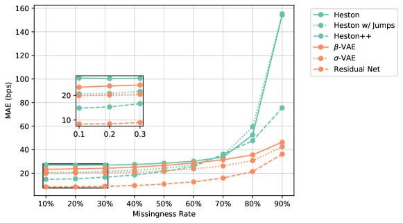
Figure 14: Mean absolute error (MAE) measured in bps on the test between imputed and masked out data for varying levels of missingness. $\sigma$-VAE uses VAE with traditional MLP blocks and “Residual Net” is a $\sigma$-VAE with residual blocks.

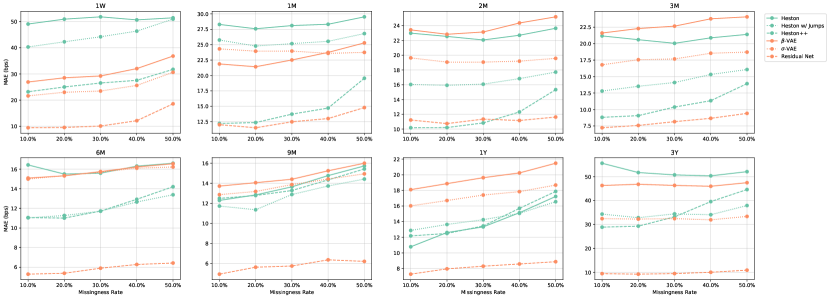
Figure 15: Mean absolute error (MAE) measured in bps on the test between imputed and masked out data for varying levels of missingness and different tenors. $\sigma$-VAE uses VAE with traditional MLP blocks and “Residual Net” is a $\sigma$-VAE with residual blocks.

7.2.1 $\sigma$-VAE and Residual Blocks

For our first set of results, we compare the three baseline models against $\beta$-VAE ($\beta=1$) with traditional MLP blocks, $\sigma$-VAE with traditional MLP blocks, and $\sigma$-VAE with residual connections. First, in Figure 15, we see that Heston is outperformed by Heston with Jumps and Heston++. Further, Heston++ outperforms across all missingness rates except around 70%. Next, we see that $\sigma$-VAE outperforms $\beta$-VAE; similar to our observation in Section 4, these models are equivalent for a specific choice of $\beta$ given $\sigma$ with the key difference that the $\sigma$ in $\sigma$-VAE did not need to be tuned.

Similar to previous findings (Bergeron et al., 2022), the $\sigma$-VAE outperforms Heston with the largest gap in performance at higher rates of missingness; this observation holds true for Heston with jumps. However, deeper analysis in Figure 15 where the results are broken down by tenors makes it clear that the $\sigma$-VAE outperforms Heston with jumps due to the smaller tenors (e.g., one week and one month) but is severely outperformed in the two, three, and six month tenors.

Further, Heston++ outperforms $\sigma$-VAE for missingness rates less than 50% (Figure 15), with the gap being much larger in certain tenors (Figure 15).

Finally, using residual blocks significantly outperforms all other models across missingness rates with the MAE dropping by more than half for 10% missingness rate (19.9 bps without residual blocks to 8.4 bps with residual blocks, Figure 15). Further, at the tenor level, the residual network outperforms all models except with the Heston++ slightly outperforming in the two months tenor at the 10-30% missingness rate.

7.2.2 $\Sigma$-VAE and IWAE

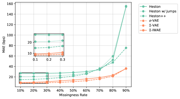
Figure 16: Mean absolute error (MAE) measured in bps on the test between imputed and masked out data for varying levels of missingness. All VAEs use residual blocks.

For our second set of results, we compare the best model in the previous section ($\sigma$-VAE with residual blocks) with $\Sigma$-VAE (where the noise $\sigma_{x}$ is a function of $z$) and $\Sigma$-IWAE. In Figure 16, we see that the imputation performance of $\Sigma$-VAE is nearly identical to $\sigma$-VAE; while we might expect the performance to improve, the main intention of using $\Sigma$-VAE is to improve the uncertainty estimates which we analyze in the next section. Interestingly, $\Sigma$-IWAE performs worse in terms of imputation performance; since IWAE loss has less bias than VAE loss, we suspect the degradation in performance might be from overfitting. Future work might explore hyperparameter tuning more thoroughly to improve the IWAE.

Further, in Appendix C, we see that, while the $\Sigma$-VAE is comparable to $\sigma$-VAE on AUDUSD, $\Sigma$-VAE performs similar to $\sigma$-VAE without residuals in low missingness regimes for USDMXN in the validation set, but much better (similar to $\sigma$-VAE with Residuals) in the test set.

7.2.3 Reconstruction of Observed Data

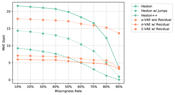
Figure 17: Mean absolute error (MAE) measured in bps on the test between imputed and observed data for varying levels of missingness.

Along with the ability to fill in missing data, a requirement of calibrating to market data is to be able to faithfully reproduce the observations from the market. In Figure 17, we compare the MAE in bps on the observed data for our baselines and three VAE variants. In the low missingness regimes, we can see that the VAEs with residual networks is better able to reproduce the observed data. The classical models performs worse because they do not have a sufficient number of parameters to fit the data.

Interestingly, in the high missingness regimes, the classical models (specifically Heston++) has a significantly lower error rate. This is to be expected since the fitting procedure is aimed at reconstructing the observed data as accurately as possible and the classical models have enough parameters to fit perfectly. The reason the VAE does not have a lower error rate is because of our distributional imputation algorithm. The goal of the algorithm is to not perfectly reconstruct the observed data, but to infer the posterior that balances the prior as well as the reconstruction term. The trade-off between the two terms is a function of the learned $\sigma$, i.e., the noisiness of the data: the more noisy the data (the higher the $\sigma$), the less accurate of a reconstruction. This can be interpreted as the distributional imputation algorithm regularizing the imputation to balance the fact that there is not a lot of observed data.

7.3 Distributional Results

	Negative ELBO ($\downarrow$)
Model	Train	Validation
$\sigma$-VAE (No Residual)	$27.0$	$39.2$
$\sigma$-IWAE (No Residual)	$12.9$	$50.4$
$\sigma$-VAE (Residual)	$-6.9$	$24.7$
$\sigma$-IWAE (Residual)	$-19.8$	$67.6$
$\Sigma$-VAE (Residual)	$-19.1$	$\mathbf{9.4}$
$\Sigma$-IWAE (Residual)	$\mathbf{-28.1}$	${12.3}$

Table 1: Comparison of Negative ELBO on validation set for different VAEs.

In Table 1, we compare the negative ELBO (approximate the negative log likelihood, or, in other words, the distributional performance) for different training methodologies for VAEs We see that consistently changing to an importance weighted loss hurts performance in the validation set. However, we see the training loss improves; thus, our results are not inconsistent with the fact that IWAEs have less bias and the simulated data example in Section 5.2.

We can see that along with the improvement in imputation that we saw in the previous section for residual networks, we see an improve in the negative ELBO. Further, while there was not an improvement in terms of imputation performance for $\Sigma$-VAE, there was an improvement in terms of negative ELBO.

While negative ELBO is a proper scoring rule (i.e., a metric that reaches its minimum value by only the optimal model) (Brier, 1950), we further explore evaluation with a more intuitive metric. Intuitively, we would like the predicted variance to be larger when the model makes larger errors, or, more rigorously, when the model predicts a variance of $\sigma^{2}$, then the average squared error should be $\sigma^{2}$. In Figure 18, we evaluate our model against this property. We expect the error-bars to overlap with the $y=x$ line. We have two observations:

1. The $\Sigma$-VAE has more variance in its predicted variance than $\vec{\sigma}$-VAE, which has more variance than $\sigma$-VAE. While the $\sigma$-VAE was homoscedastic output noise, there still is a range of predicted variances is because the imputation algorithm from Section 6.1 (Equation 6.1) integrates over multiple values of $z$.

2. The predicted variance by $\sigma$-VAE and $\vec{\sigma}$-VAE is overestimating the true variance; the $\Sigma$-VAE is more accurate with some overestimation near $10^{-7}$.

Figure 18 shows the value of uncertainty estimates: a model trained to output accurate uncertainty estimates can give practitioners better insight into the accuracy of the model. Specifically, the model’s predicted variance is a way for the model to convey its prediction of how accurate imputation prediction is.

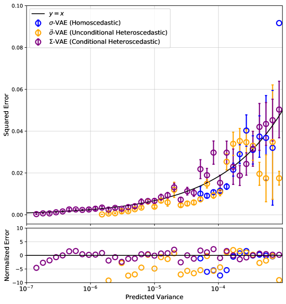
Figure 18: Performance of variance prediction by VAEs. We compare using a scalar for the output noise (homoscedastic), a vector of the output noise (unconditional heteroscedastic), and noise conditional on $z$ (conditional heteroscedastic). The error-bars in the top plot show the mean and standard error of the squared errors in each bin. The bottom plot shows the distance of the mean from $y=x$ line normalized by the standard error. The $y=x$ line is curved because the $x$-axis is log-scaled.

7.4 Additional Experiments

7.4.1 Hyperparameter Tuning

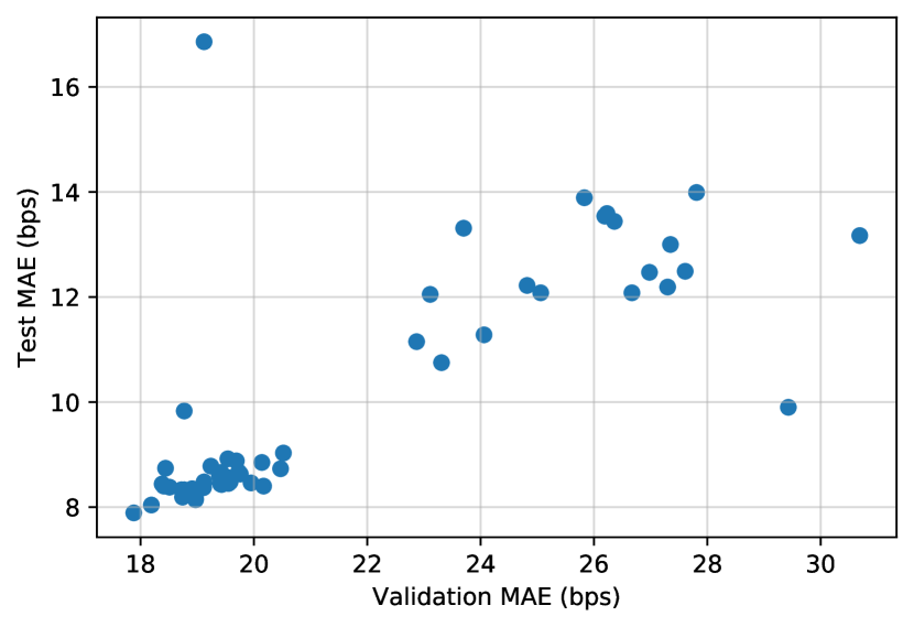
(a) Comparison of MAE for validation and test

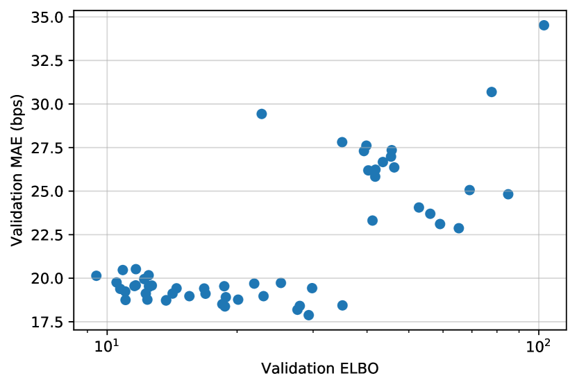
(b) Comparison of MAE and ELBO for validation

Figure 19: Comparison of $\Sigma$-VAE performance across hyperparameters on AUDUSD surfaces.

As we noted earlier, we hyperparameter tuned all VAEs across 64 different configurations with different hidden sizes (64 and 128), the number of layers (2, 3, and 4), dropout rates (0.1, 0.2, 0.3, and 0.4), and the embedding sizes (32 and 64). A question we asked was, “How correlated is the performance on the validation set to the performance on the test set?” In Figure 19(a), we compare the performance for AUDUSD with 10% missingness rate. We see there is a strong correlation (0.77) between the two MAEs, with the optimal model in the validation set being the optimal model for the test set. In other words, Figure 19(a) implies that we are not overfitting to the validation set.

Further, we hyperparameter tuned the validation ELBO and accordingly asked, “Is optimizing for ELBO a good proxy for imputation performance, or, in other words, how correlated is the validation ELBO and validation MAE?” In Figure 19(b), we see there is a strong correlation (0.77 again) between the two metrics. However, we see that the validation MAE does not seem to improve for ELBO less than 50; this implies that, for validation ELBO, the improvement is coming from the accurate uncertainty estimation. In other words, Figure 19(a) implies that using the validation ELBO is an effective metric to tune.

7.4.2 Choosing Embedding Size

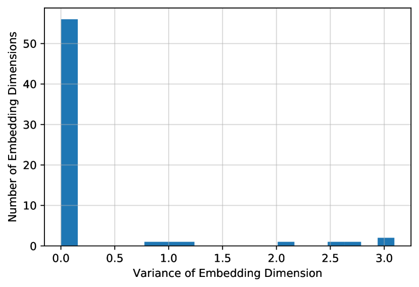
(a) Histogram of variances

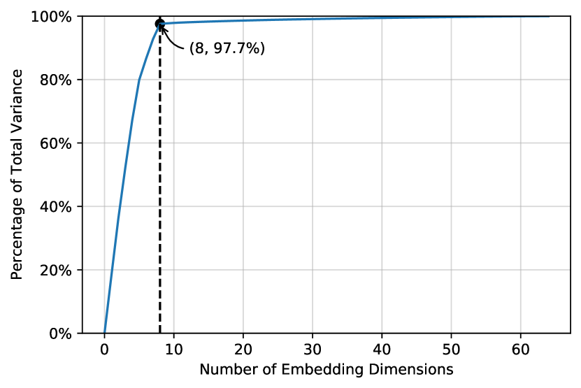
(b) Skree plot of variances of embeddings

Figure 20: Analysis of posterior collapse in VAEs for $\Sigma$-VAE where the embedding dimension is 64.

A common question when using VAEs is “how many embedding dimensions to use?” The embedding size tends to be a common hyperparameter that is tuned (e.g., Bergeron et al. (2022); Sokol (2022)). We show in Figure 20 that the number of embedding dimensions is automatically tuned by the VAE. Prior works (e.g., Burda et al. (2015); Vahdat and Kautz (2020); Lucas et al. (2019)) have discussed the problem of “posterior collapse” where some latent dimensions are independent of the inputs. In other words, the mean of the posterior for some latent dimensions is zero for all samples (assuming $\mathcal{N}(0,I)$ prior). To evaluate the number of dimensions that have collapsed, we compute $\mu_{\mathbf{z}|\mathbf{x}}$ for each data point and then take the variance of each dimension. In Figure 20(a), we plot the histogram of the variances, and we see there is clear separation between some dimensions being very close to zero and others larger than 0.5. In Figure 20(b), we plot the total variance of the embeddings explained by each dimension and see that 8 explains 97.7% of the variance in $\mu_{\mathbf{z}|\mathbf{x}}$. In other words, the VAE learned without supervision to use only eight embedding dimensions.

7.4.3 Arbitrage Evaluation

	AUDUSD	EURUSD	USDCAD	GBPCAD	USDMXN
$\sigma$-VAE w/o Residual	$35.8\pm 0.1$	$24.5\pm 0.1$	$34.6\pm 0.1$	$21.6\pm 0.1$	$38.6\pm 0.1$
$\sigma$-VAE w/ Residual	$78.9\pm 0.1$	$\mathbf{73.7\pm 0.1}$	$87.7\pm 0.1$	$65.9\pm 0.1$	$\mathbf{76.8\pm 0.1}$
$\Sigma$-VAE w/ Residual	$\mathbf{81.8\pm 0.1}$	${73.2\pm 0.1}$	$\mathbf{91.2\pm 0.1}$	$\mathbf{68.2\pm 0.1}$	${72.2\pm 0.1}$
Real	$100.0$	100.0	100.0	99.9	99.9

Table 2: Percentage of surfaces which contain no-arbitrage opportunities, evaluated on 100K samples.

One major component in option pricing and volatility surface construction is ensuring no-arbitrage, i.e., the prices given from the model do not allow for non-zero probability of making money from no money. Many works (e.g., Davis and Hobson (2007); Roper (2010)) have characterized the conditions required for an option surface to be arbitrage free; the conditions can be summarized as requiring positive implied volatility, monotonicity in time to maturity (calendar arbitrage condition), convex along the strike dimension (butterfly arbitrage condition), and boundary conditions.

For this work, since our surface has a discrete number of observations, we use:

Theorem 7.1.

A set of call prices $\{p_{k,t}\}$ are consistent with no arbitrage (assuming the forward price is equal for all $t$) if and only if

• $K_{k,t}=K_{k^{\prime},t^{\prime}}$ and $t<t^{\prime}$ implies $p_{k,t}<p_{k^{\prime},t^{\prime}}$

• $\forall k,\forall t$,

  $$\sup_{t^{\prime}\geq t}\sup_{\{k^{\prime}\mathrel{\mathop{\mathchar 58\relax}}K_{k^{\prime},t^{\prime}}<K_{k,t}\}}\frac{p_{k,t}-p_{k^{\prime},t^{\prime}}}{K_{k,t}-K_{k^{\prime},t^{\prime}}}\leq\min\left(0,\inf_{t^{\prime\prime}\geq t}\inf_{\{k^{\prime\prime}\mathrel{\mathop{\mathchar 58\relax}}K_{k^{\prime\prime},t^{\prime\prime}}>K_{k,t}\}}\frac{p_{k^{\prime\prime},t^{\prime\prime}}-p_{k,t}}{K_{k^{\prime\prime},t^{\prime\prime}}-K_{k,t}}\right)$$

where we use $K_{k,t}$ to denote strike at a given strike-index $k$ and tenor $t$. Theorem 7.1 gives us a simple algorithm to run on generated volatility surfaces (converted to call prices space) to test for arbitrage.

In Table 2, we compute the percentage of surfaces generated by different VAEs that contain an arbitrage. By construction, our baseline models are guaranteed to be no arbitrage and thus, we do not include them in our table. For each model, we sample 100K times (using the algorithm explained in Section 3.1) and compute the percentage of which have no-arbitrage. We can see that there’s a massive improvement by including residual connections and some benefits by using $\Sigma$-VAE over $\sigma$-VAE, but the result is not consistent across all currency pairs. Note that we do not include any constraints during training to enforce no-arbitrage conditions, the performance we see is from what the model learned from the data. Further, we note that the easiest way to perform well on this task is to simply memorize the training set. However, this form of overfitting would prevent the model from being able to perform accurate imputations on the validation and test set.

8 Conclusion

In this work, we introduce a simple set of tricks to improve the imputation performance of VAEs on FX volatility surfaces. With these, we close the gap between the usage of VAEs in imputing volatility surfaces and the usage of VAEs for imputation in the machine learning community. Namely, we show using residual networks leads to stronger performance, $\beta$-VAE is not necessary for training strong VAEs, and VAEs can give accurate uncertainty estimates. Further, we show that using stronger baselines can help discover gaps in performance and accurately measuring the efficacy of an approach requires thorough comparison against classical approaches.

Appendix A Sampling Noise

In this section, using the models trained in Section 4, we show the importance of sampling from $p(\mathbf{x}|\mathbf{z})$ (using $\sigma_{x}$) instead of simply using the mean ($\mathbb{E}[\mathbf{x}|\mathbf{z}]$). In Figure 22, we show the generations when $\sigma_{x}$ is set to $0$; as expected, the variance observed in the data is not captured by these generations except with very low beta.

Figure 21: Mixture of two Gaussians.

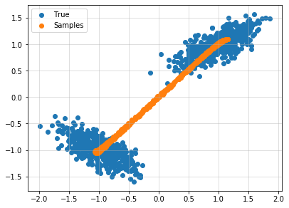
(a) $\beta=1$

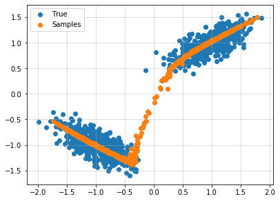
(b) $\beta=0.1$

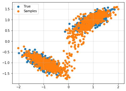
(c) Learnable $\beta$

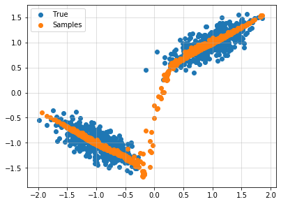
(d) $\sigma$-VAE

Figure 22: Comparison of generations by different VAEs with $\sigma_{x}$ set to zero.

Appendix B Model Details

B.1 VAE Residual Architecture

While we showed the diagram of our architecture in Section 5.3, here, we write the architecture mathematically in order to aid in re-implementing our architecture. Specifically, the VAE architecture in Figure 10 is:

$$\mathbf{h}_{1,e} =W_{1}\mathbf{x}$$

$$\mathbf{h}_{2,e} =\mathbf{h}_{1,e}+W_{3}\sigma(W_{2}\ \text{LN}(\mathbf{h}_{1,e}))$$

$$\mathbf{h}_{3,e} =\mathbf{h}_{2,e}+W_{5}\sigma(W_{4}\ \text{LN}(\mathbf{h}_{2,e}))$$

$$\mu_{\mathbf{z}|\mathbf{x}}=W_{6,1}\mathbf{h}_{3,e} \qquad\sigma_{\mathbf{z}|\mathbf{x}}=\text{Softplus}(W_{6,2}\mathbf{h}_{3,e})$$

$$\mathbf{z} \sim\mathcal{N}(\mu_{\mathbf{z}|\mathbf{x}},\sigma_{\mathbf{z}|\mathbf{x}})$$

$$\mathbf{h}_{1,d} =W_{7}\mathbf{z}$$

$$\mathbf{h}_{2,d} =\mathbf{h}_{1,d}+W_{9}\sigma(W_{8}\ \text{LN}(\mathbf{h}_{1,d}))$$

$$\mathbf{h}_{3,d} =\mathbf{h}_{2,d}+W_{11}\sigma(W_{10}\ \text{LN}(\mathbf{h}_{2,d}))$$

$$\mu_{\mathbf{x}|\mathbf{z}}=W_{12,1}\mathbf{h}_{3,d} \qquad\sigma_{\mathbf{x}|\mathbf{z}}=\text{Softplus}(W_{12,2}\mathbf{h}_{3,d})$$

where $\mathbf{x}\in\mathbb{R}^{d}$, $\mathbf{z}\in\mathbb{R}^{e}$, $W_{1}\in\mathbb{R}^{h\times d}$, $W_{2},W_{3},W_{4},W_{5},W_{8},W_{9},W_{10},W_{11}\in\mathbb{R}^{h\times h}$, $W_{6,1},W_{6,2}\in\mathbb{R}^{e\times h}$, $W_{7}\in\mathbb{R}^{h\times e}$, and $W_{12,1},W_{12,2}\in\mathbb{R}^{d\times h}$. For ease of reading, we dropped all bias terms, LN refers to Layer Norm (Ba et al., 2016), and $\sigma$ is SiLU (Ramachandran et al., 2018).

B.2 Experimental Details for Section 4 and Section 5.2

For the data, we sampled from a mixture of two Gaussians with equal probability:

$$\mathcal{N}\left(\begin{bmatrix}1.0\\ 1.0\end{bmatrix},\begin{bmatrix}0.1&0.05\\ 0.05&0.05\end{bmatrix}\right)\qquad\mathcal{N}\left(\begin{bmatrix}-1.0\\ -1.0\end{bmatrix},\begin{bmatrix}0.1&-0.05\\ -0.05&0.05\end{bmatrix}\right)$$

We sampled 1K data points for training.

For our architecture, we used residual networks where, using the notation in Section B.1, $d=2$, $h=64$, and $e=4$. For training, we used the Adam optimizer (Kingma and Ba, 2015) with a learning rate of 1e-4 and no weight decay and trained with a batch size of 64 for 100K updates (gradient steps). However, since the experiments in Section 4 are for $\sigma-VAE$ and $\beta$-VAE, the layer for $\sigma_{\mathbf{x}|\mathbf{z}}$ is not used.

B.3 Experimental Details for Section 5.1

For the data, we sampled from a mixture of two Gaussians with equal probability:

$$\mathcal{N}\left(\begin{bmatrix}1.0\\ 1.0\end{bmatrix},\begin{bmatrix}0.4&0.05\\ 0.05&0.05\end{bmatrix}\right)\qquad\mathcal{N}\left(\begin{bmatrix}-1.0\\ -1.0\end{bmatrix},\begin{bmatrix}0.4&-0.05\\ -0.05&0.05\end{bmatrix}\right)$$

We sampled 1K data points for training.

For our architecture, we used residual networks where, using the notation in Section B.1, $d=2$, $h=64$, and $e=4$. For training, we used the Adam optimizer (Kingma and Ba, 2015) with a learning rate of $1e{-4}$, no weight decay, and trained with a batch size of 64 for 100K updates (gradient steps).

B.4 Experimental Details for Section 5.3

For the data, we sampled from a mixture of eight Gaussians with equal probability using the code from the residual flow codebase. We sampled 1K data points for training.

For our architecture, we used residual networks where, using the notation in Section B.1, $d=2$, $h=64$, and $e=4$. For training, we used the Adam optimizer (Kingma and Ba, 2015) with a learning rate of $1e{-4}$, no weight decay, and trained with a batch size of 64 for 100K updates (gradient steps).

B.5 Model Details for Section 7

The data we used is described in Section 7.1.1.

For each model, we tuned the hidden size (64 and 128), the number of layers (2, 3, and 4), dropout rate (0.1, 0.2, 0.3, and 0.4), and the embedding size (32 and 64). For training, we used the Adam optimizer (Kingma and Ba, 2015) weight decay of 1e-5 and trained with a batch size of 64 for 100K updates (gradient steps). For the learning rate, we used a linear warmup from $1e{-7}$ to $2e{-4}$ over 5K steps and then halved the learning rate after 50K steps.

For evaluation, we retrain the encoder on the corresponding dataset with the Adam optimizer (Kingma and Ba, 2015) with no weight decay and with a learning rate of $2e{-4}$ where we used a linear warmup for 100 steps. We then trained for 10K steps with a batch size 32 and setting k=50 (even when we trained our model with $k=1$). To remove sources of randomness, we set the dropout rates to zero. Finally, for imputation, using the algorithm in Section 6, we use 10K importance weighting samples.

Appendix C MAE on All Surfaces

	10%	20%	30%	40%	50%	60%	70%	80%	90%
Heston	27.05	26.85	26.95	27.41	28.50	30.19	33.77	52.52	154.28
Heston w/ Jumps	20.65	20.76	21.61	22.46	24.25	26.95	35.16	59.47	155.31
Heston++	14.85	15.31	16.64	18.56	21.60	25.72	36.18	47.61	75.53
$\sigma$-VAE w/o Residual	19.88	20.15	20.46	20.92	22.01	23.73	26.18	30.72	42.52
$\sigma$-VAE w/ Residual	8.40	8.47	8.94	9.54	10.87	12.68	15.95	21.47	36.24
$\Sigma$-VAE w/ Residual	8.65	8.97	9.21	9.71	11.18	12.99	16.13	21.18	35.77

(a) AUDUSD

	10%	20%	30%	40%	50%	60%	70%	80%	90%
Heston	20.81	20.75	20.94	21.40	22.35	23.52	28.10	47.26	150.52
Heston w/ Jumps	20.39	20.86	21.25	22.48	23.38	27.08	34.18	59.28	151.24
Heston++	12.85	13.06	14.03	14.93	16.96	21.95	29.46	41.47	70.09
$\sigma$-VAE w/o Residual	15.36	15.47	15.91	16.41	17.04	18.54	20.69	24.67	37.31
$\sigma$-VAE w/ Residual	7.50	7.54	7.97	8.75	9.97	12.25	15.57	20.08	34.74
$\Sigma$-VAE w/ Residual	8.48	8.31	8.72	9.56	11.01	12.29	15.97	20.60	37.31

(b) EURUSD

	10%	20%	30%	40%	50%	60%	70%	80%	90%
Heston	20.03	20.54	20.96	21.11	21.70	22.69	25.31	44.07	153.74
Heston w/ Jumps	17.20	18.40	19.28	20.62	22.30	26.34	36.69	61.34	162.48
Heston++	13.56	14.26	14.87	15.86	18.09	22.17	29.87	46.28	89.90
$\sigma$-VAE w/o Residual	16.25	16.53	16.63	16.89	17.51	18.98	20.69	24.18	33.49
$\sigma$-VAE w/ Residual	6.10	6.57	6.94	7.62	8.68	10.65	13.54	18.36	28.46
$\Sigma$-VAE w/ Residual	6.32	6.69	6.87	7.24	8.42	9.76	12.26	17.16	28.98

(c) USDCAD

	10%	20%	30%	40%	50%	60%	70%	80%	90%
Heston	22.71	22.44	22.86	23.20	24.05	25.41	29.24	44.88	157.29
Heston w/ Jumps	21.11	20.82	21.64	22.39	24.26	26.87	34.85	58.74	153.90
Heston++	13.52	14.18	15.41	16.93	19.87	23.73	32.63	46.79	79.29
$\sigma$-VAE w/o Residual	17.22	17.26	17.49	17.80	18.47	19.97	21.90	25.21	34.10
$\sigma$-VAE w/ Residual	6.90	7.39	7.91	8.57	9.78	12.06	15.08	20.34	31.09
$\Sigma$-VAE w/ Residual	8.54	8.66	9.12	9.62	10.96	12.59	15.78	21.42	33.16

(d) GBPUSD

	10%	20%	30%	40%	50%	60%	70%	80%	90%
Heston	36.05	36.68	37.07	37.47	38.62	40.63	45.07	67.27	211.61
Heston w/ Jumps	28.72	29.63	30.18	30.20	32.56	36.58	46.28	77.08	197.17
Heston++	30.39	32.33	32.82	33.78	37.86	44.11	59.06	96.79	201.93
$\sigma$-VAE w/o Residual	48.00	47.78	48.00	48.47	49.37	51.46	53.44	57.62	67.66
$\sigma$-VAE w/ Residual	12.68	12.89	13.51	14.50	16.21	20.08	26.23	37.15	58.81
$\Sigma$-VAE w/ Residual	16.33	16.64	17.16	18.24	20.15	23.77	29.34	39.54	61.65

(e) USDMXN

Table 3: Mean absolute error (MAE) measured in bps on the test set for varying levels of missingness for different surfaces.

	10%	20%	30%	40%	50%	60%	70%	80%	90%
Heston	37.69	39.70	40.77	41.84	43.78	46.50	49.17	71.64	184.60
Heston w/ Jumps	32.28	34.17	34.91	38.29	40.45	45.01	54.40	77.75	162.26
Heston++	24.96	27.21	28.05	29.53	32.92	40.36	54.64	74.41	103.35
$\sigma$-VAE w/o Residual	29.55	32.72	32.75	33.28	34.15	36.98	41.88	51.76	73.40
$\sigma$-VAE w/ Residual	15.61	16.94	16.80	17.57	18.96	21.85	27.65	37.82	61.23
$\Sigma$-VAE w/ Residual	20.25	21.52	22.24	23.21	24.14	26.29	30.87	39.00	60.56

(a) AUDUSD

	10%	20%	30%	40%	50%	60%	70%	80%	90%
Heston	26.46	27.35	27.59	28.45	28.67	30.84	33.73	53.53	161.72
Heston w/ Jumps	22.86	24.74	26.13	26.32	27.61	30.47	38.14	62.53	147.85
Heston++	15.48	16.48	17.13	18.78	20.46	25.13	31.73	48.63	83.33
$\sigma$-VAE w/o Residual	28.71	29.05	29.56	29.77	30.52	32.56	35.35	42.51	57.60
$\sigma$-VAE w/ Residual	10.97	11.49	11.76	12.77	13.87	17.34	23.03	33.33	51.04
$\Sigma$-VAE w/ Residual	11.64	12.80	13.58	14.55	15.32	18.49	22.28	31.77	50.82

(b) EURUSD

	10%	20%	30%	40%	50%	60%	70%	80%	90%
Heston	26.67	28.03	27.75	28.44	28.98	31.18	34.43	55.45	177.47
Heston w/ Jumps	24.68	25.90	25.81	26.83	30.38	34.23	46.11	69.07	149.83
Heston++	16.54	17.79	18.24	19.99	22.85	28.54	34.67	54.23	99.33
$\sigma$-VAE w/o Residual	25.51	26.84	27.43	27.59	28.26	30.16	32.43	39.64	57.21
$\sigma$-VAE w/ Residual	10.73	11.43	11.91	13.29	14.61	18.56	23.46	33.29	51.70
$\Sigma$-VAE w/ Residual	10.87	12.01	12.73	13.47	14.36	17.33	20.82	30.23	51.80

(c) USDCAD

	10%	20%	30%	40%	50%	60%	70%	80%	90%
Heston	36.41	37.47	38.07	38.88	40.07	42.07	46.53	72.97	173.81
Heston w/ Jumps	30.77	32.03	33.07	34.06	37.37	41.29	50.93	76.10	162.46
Heston++	19.65	21.17	22.45	23.59	28.17	34.76	46.42	69.64	94.34
$\sigma$-VAE w/o Residual	29.68	30.55	31.45	31.65	32.19	34.00	37.29	43.03	57.29
$\sigma$-VAE w/ Residual	13.24	13.65	13.97	14.92	15.93	19.56	25.29	34.23	51.81
$\Sigma$-VAE w/ Residual	18.02	19.16	19.85	20.80	22.00	25.08	29.88	38.34	55.36

(d) GBPUSD

	10%	20%	30%	40%	50%	60%	70%	80%	90%
Heston	67.06	72.22	71.64	73.20	76.05	81.40	90.28	127.06	306.38
Heston w/ Jumps	58.01	62.69	61.45	63.48	66.64	74.71	95.46	147.10	309.41
Heston++	52.44	56.96	58.04	61.37	67.74	80.33	107.27	158.56	291.70
$\sigma$-VAE w/o Residual	45.81	47.94	48.08	49.03	51.55	56.39	63.80	80.97	124.04
$\sigma$-VAE w/ Residual	20.45	21.82	22.40	24.24	26.65	31.01	39.64	57.77	106.03
$\Sigma$-VAE w/ Residual	48.91	57.30	59.19	61.74	63.34	68.83	76.39	94.68	138.18

(e) USDMXN

Table 4: Mean absolute error (MAE) measured in bps on the validation set for varying levels of missingness for different surfaces.

Appendix D MAE on Observed Data in All Surfaces

	10%	20%	30%	40%	50%	60%	70%	80%	90%
Heston	21.64	21.36	21.07	20.73	19.88	18.33	16.59	12.25	3.55
Heston w/ Jumps	14.38	14.08	13.55	13.03	12.07	10.38	8.41	4.97	0.91
Heston++	9.23	8.85	8.30	7.61	6.52	4.97	3.08	1.22	0.07
$\sigma$-VAE w/o Residual	17.85	17.72	17.55	17.40	17.15	16.38	15.91	15.29	13.65
$\sigma$-VAE w/ Residual	5.99	5.89	5.80	5.82	5.47	5.14	4.89	4.63	3.23
$\Sigma$-VAE w/ Residual	7.09	7.01	6.89	6.78	6.55	6.20	5.76	5.69	3.72

(a) AUDUSD

	10%	20%	30%	40%	50%	60%	70%	80%	90%
Heston	17.23	17.04	16.69	16.38	15.84	14.93	13.38	10.04	3.76
Heston w/ Jumps	15.27	14.96	14.53	14.01	13.18	11.93	10.12	7.22	2.13
Heston++	7.97	7.68	7.51	6.76	5.96	4.72	3.11	1.37	0.08
$\sigma$-VAE w/o Residual	13.72	13.71	13.66	13.57	13.54	13.41	13.55	13.74	13.90
$\sigma$-VAE w/ Residual	5.44	5.31	5.26	5.15	5.35	4.93	4.91	4.50	3.34
$\Sigma$-VAE w/ Residual	6.84	6.69	6.67	6.57	6.63	6.22	6.01	5.53	4.05

(b) EURUSD

	10%	20%	30%	40%	50%	60%	70%	80%	90%
Heston	16.71	16.34	15.96	15.59	14.97	13.83	12.20	9.36	3.45
Heston w/ Jumps	12.44	12.08	11.72	11.31	10.66	9.82	8.77	6.87	2.60
Heston++	8.35	7.85	7.36	6.77	5.85	4.43	2.74	1.10	0.09
$\sigma$-VAE w/o Residual	14.07	13.97	13.85	13.78	13.67	13.38	13.23	13.34	13.08
$\sigma$-VAE w/ Residual	4.40	4.33	4.35	4.41	4.26	4.22	4.15	4.02	3.06
$\Sigma$-VAE w/ Residual	5.16	5.06	4.94	4.87	4.68	4.46	4.10	3.73	2.67

(c) USDCAD

	10%	20%	30%	40%	50%	60%	70%	80%	90%
Heston	18.64	18.47	18.17	17.65	17.05	15.99	14.32	10.59	3.09
Heston w/ Jumps	15.17	14.88	14.36	13.54	12.48	11.31	9.19	6.05	1.19
Heston++	8.81	8.48	7.95	7.39	6.54	5.10	3.23	1.43	0.05
$\sigma$-VAE w/o Residual	15.18	15.15	15.07	14.86	14.73	14.05	13.45	12.51	10.87
$\sigma$-VAE w/ Residual	5.05	5.04	4.96	5.01	4.87	4.76	4.53	4.31	2.98
$\Sigma$-VAE w/ Residual	7.17	7.13	7.12	7.04	6.84	6.58	6.47	6.25	5.28

(d) GBPUSD

	10%	20%	30%	40%	50%	60%	70%	80%	90%
Heston	28.66	28.24	27.60	26.96	25.84	24.10	21.05	15.40	6.03
Heston w/ Jumps	19.93	19.26	18.46	17.57	16.29	14.12	10.79	6.30	1.02
Heston++	18.73	17.56	16.42	15.05	12.92	9.91	6.37	2.62	0.18
$\sigma$-VAE w/o Residual	40.87	40.39	39.76	38.87	37.95	36.19	33.51	29.98	22.96
$\sigma$-VAE w/ Residual	8.34	8.20	8.07	7.90	7.74	7.47	7.16	6.98	5.26
$\Sigma$-VAE w/ Residual	12.63	12.62	12.71	12.70	12.60	12.45	12.31	11.78	8.59

(e) USDMXN

Table 5: Mean absolute error (MAE) measured in bps on the test set for observed data for varying levels of missingness for different surfaces.

	10%	20%	30%	40%	50%	60%	70%	80%	90%
Heston	32.67	32.17	31.39	30.87	29.77	27.49	24.12	17.40	6.15
Heston w/ Jumps	24.86	24.20	23.38	22.84	21.69	19.35	15.38	9.84	2.51
Heston++	16.71	15.91	15.09	14.36	12.72	10.78	6.82	3.14	0.38
$\sigma$-VAE w/o Residual	28.44	27.97	27.83	27.58	27.11	26.63	26.10	25.43	23.06
$\sigma$-VAE w/ Residual	10.88	10.58	10.29	10.06	9.73	9.21	8.49	7.30	4.89
$\Sigma$-VAE w/ Residual	17.64	17.20	16.96	16.70	16.83	16.61	14.99	12.12	10.13

(a) AUDUSD

	10%	20%	30%	40%	50%	60%	70%	80%	90%
Heston	22.24	21.75	21.16	20.44	19.75	18.44	16.59	12.39	4.14
Heston w/ Jumps	16.96	16.54	16.15	15.36	14.45	12.71	10.92	6.71	2.29
Heston++	9.77	9.22	8.78	8.04	7.02	5.84	3.83	1.66	0.14
$\sigma$-VAE w/o Residual	24.99	24.81	24.55	24.48	24.24	24.28	23.49	23.07	20.91
$\sigma$-VAE w/ Residual	7.47	7.47	7.36	7.22	7.33	7.32	7.35	6.97	4.52
$\Sigma$-VAE w/ Residual	10.63	10.53	10.43	10.28	10.21	10.18	9.34	8.17	5.08

(b) EURUSD

	10%	20%	30%	40%	50%	60%	70%	80%	90%
Heston	22.24	21.70	21.34	20.84	20.11	18.80	17.21	12.93	4.23
Heston w/ Jumps	18.60	17.92	17.66	17.18	16.39	14.43	13.30	9.36	2.64
Heston++	11.05	10.64	10.19	9.37	8.25	6.93	4.38	2.11	0.26
$\sigma$-VAE w/o Residual	22.81	22.61	22.30	22.24	22.07	22.17	22.39	22.27	21.89
$\sigma$-VAE w/ Residual	7.37	7.27	7.25	7.42	7.26	7.32	7.35	6.72	4.77
$\Sigma$-VAE w/ Residual	9.32	9.26	9.23	9.06	8.92	8.81	8.62	7.76	4.99

(c) USDCAD

	10%	20%	30%	40%	50%	60%	70%	80%	90%
Heston	31.06	30.50	29.84	29.18	28.05	25.86	23.22	17.55	6.14
Heston w/ Jumps	23.26	22.61	21.82	20.89	19.72	17.57	14.17	10.01	2.83
Heston++	14.03	13.70	13.23	12.60	11.33	9.54	6.60	3.41	0.28
$\sigma$-VAE w/o Residual	27.01	26.79	26.22	26.11	25.81	24.95	23.39	21.87	17.73
$\sigma$-VAE w/ Residual	8.82	8.66	8.47	8.26	7.92	7.55	7.37	6.56	4.76
$\Sigma$-VAE w/ Residual	16.10	16.14	15.98	15.84	15.94	15.76	14.41	12.95	11.52

(d) GBPUSD

	10%	20%	30%	40%	50%	60%	70%	80%	90%
Heston	59.08	57.82	56.91	55.71	53.54	49.82	44.38	35.12	11.90
Heston w/ Jumps	45.86	44.10	44.15	42.38	40.42	36.69	31.75	24.08	6.97
Heston++	38.19	36.53	34.91	32.61	29.74	25.08	17.70	10.06	1.54
$\sigma$-VAE w/o Residual	41.27	40.81	40.47	40.03	39.12	38.47	37.56	36.58	33.25
$\sigma$-VAE w/ Residual	14.43	13.98	13.46	13.00	11.98	11.32	10.14	9.61	6.65
$\Sigma$-VAE w/ Residual	47.76	48.36	48.85	49.90	52.35	54.77	56.70	57.82	62.55

(e) USDMXN

Table 6: Mean absolute error (MAE) measured in bps on the validation set for observed data for varying levels of missingness for different surfaces.

Appendix E MAE for Different Tenors

Tenor	1W	1M	2M	3M	6M	9M	1Y	3Y
Heston	49.09	28.29	22.98	21.18	16.43	12.30	10.78	55.62
Heston w/ Jumps	40.31	25.76	16.03	12.80	11.04	11.74	12.88	34.36
Heston++	23.20	12.20	10.17	8.81	11.06	12.50	12.18	28.90
$\sigma$-VAE w/o Residual	21.63	24.32	19.63	16.79	14.99	12.87	16.02	32.46
$\sigma$-VAE w/ Residual	9.44	12.00	11.22	7.23	5.29	4.96	7.28	9.48
$\Sigma$-VAE w/ Residual	9.94	12.02	13.26	7.94	5.28	5.29	6.88	8.38

(a) AUDUSD

Tenor	1W	1M	2M	3M	6M	9M	1Y	3Y
Heston	38.62	26.30	19.04	14.18	10.45	11.74	15.97	29.87
Heston w/ Jumps	40.54	24.30	14.07	10.99	10.51	14.45	15.49	32.56
Heston++	18.61	11.07	9.17	8.22	9.10	9.65	11.71	25.40
$\sigma$-VAE w/o Residual	17.23	15.56	15.12	12.96	12.20	13.40	17.29	19.15
$\sigma$-VAE w/ Residual	9.23	7.75	7.29	6.47	6.07	6.67	7.37	9.16
$\Sigma$-VAE w/ Residual	10.54	7.95	10.82	5.89	6.15	6.41	8.08	11.98

(b) EURUSD

Tenor	1W	1M	2M	3M	6M	9M	1Y	3Y
Heston	37.06	24.98	16.61	13.34	9.57	11.27	14.98	32.24
Heston w/ Jumps	33.45	19.62	12.81	9.84	8.48	10.45	13.50	29.37
Heston++	21.40	9.73	9.81	8.58	9.38	10.71	12.58	26.65
$\sigma$-VAE w/o Residual	22.63	19.61	14.81	12.84	9.76	9.72	13.18	27.36
$\sigma$-VAE w/ Residual	7.73	6.18	5.25	5.14	3.90	3.78	5.98	10.87
$\Sigma$-VAE w/ Residual	7.95	5.61	7.37	4.20	3.57	3.59	4.77	13.59

(c) USDCAD

Tenor	1W	1M	2M	3M	6M	9M	1Y	3Y
Heston	41.23	28.59	19.44	18.07	12.22	9.84	13.21	38.90
Heston w/ Jumps	42.44	27.68	15.03	12.13	10.46	12.19	14.70	33.83
Heston++	21.67	12.39	9.51	9.33	10.95	11.33	10.96	22.06
$\sigma$-VAE w/o Residual	24.83	25.40	15.77	11.64	10.79	11.24	11.58	25.85
$\sigma$-VAE w/ Residual	10.65	8.73	6.48	5.58	5.20	3.69	5.64	9.05
$\Sigma$-VAE w/ Residual	14.28	11.03	11.00	5.21	4.42	2.85	4.35	14.97

(d) GBPUSD

Tenor	1W	1M	2M	3M	6M	9M	1Y	3Y
Heston	63.24	28.90	32.48	29.94	19.30	16.61	18.75	80.49
Heston w/ Jumps	45.38	30.54	22.47	18.43	15.54	20.09	23.41	54.06
Heston++	48.66	18.82	23.10	23.01	23.13	22.22	25.44	59.87
$\sigma$-VAE w/o Residual	75.09	62.48	38.86	30.70	26.49	27.07	31.59	90.88
$\sigma$-VAE w/ Residual	23.02	11.83	10.92	7.36	7.56	8.05	8.91	23.91
$\Sigma$-VAE w/ Residual	29.85	9.37	11.88	9.07	9.99	7.81	11.75	41.53

(e) USDMXN

Table 7: Mean absolute error (MAE) measured in bps on the test set for varying tenors for different surfaces with missingness rate of 10%.

Tenor	1W	1M	2M	3M	6M	9M	1Y	3Y
Heston	51.46	29.53	23.64	21.41	16.60	15.73	17.23	52.10
Heston w/ Jumps	50.98	26.81	17.71	16.07	13.38	14.43	16.55	37.94
Heston++	31.76	19.55	15.33	13.93	14.21	15.43	17.87	44.63
$\sigma$-VAE w/o Residual	30.65	23.75	19.57	18.72	16.22	14.94	18.68	33.39
$\sigma$-VAE w/ Residual	18.59	14.78	11.62	9.42	6.43	6.23	8.87	10.94
$\Sigma$-VAE w/ Residual	19.68	16.82	12.92	9.43	6.33	6.21	8.15	9.75

(a) AUDUSD

Tenor	1W	1M	2M	3M	6M	9M	1Y	3Y
Heston	39.13	27.59	19.31	16.46	12.34	14.09	18.81	30.94
Heston w/ Jumps	51.39	25.91	16.31	13.83	12.06	15.56	18.74	33.12
Heston++	23.52	16.83	12.71	11.39	11.81	12.59	15.75	31.03
$\sigma$-VAE w/o Residual	22.85	16.68	15.59	14.34	12.03	14.54	19.60	20.59
$\sigma$-VAE w/ Residual	17.15	10.47	8.31	7.78	7.40	7.64	9.23	11.75
$\Sigma$-VAE w/ Residual	20.62	12.49	10.30	7.45	6.80	7.11	9.74	13.51

(b) EURUSD

Tenor	1W	1M	2M	3M	6M	9M	1Y	3Y
Heston	39.76	25.45	17.53	14.36	10.70	12.36	17.16	36.11
Heston w/ Jumps	51.70	25.52	14.57	11.81	11.04	13.18	16.95	33.54
Heston++	24.81	15.58	12.87	12.58	13.42	13.69	16.32	35.36
$\sigma$-VAE w/o Residual	29.25	20.93	15.12	13.09	10.09	10.34	14.23	26.94
$\sigma$-VAE w/ Residual	15.28	10.07	6.27	6.00	4.92	4.69	7.09	15.09
$\Sigma$-VAE w/ Residual	14.72	9.76	7.82	5.34	4.37	4.19	5.87	15.20

(c) USDCAD

Tenor	1W	1M	2M	3M	6M	9M	1Y	3Y
Heston	43.10	29.41	19.60	17.94	12.91	12.94	17.69	38.62
Heston w/ Jumps	51.50	28.59	16.72	14.81	12.37	14.56	18.47	36.94
Heston++	28.83	18.79	14.83	13.05	13.64	14.73	16.63	38.39
$\sigma$-VAE w/o Residual	30.66	25.65	16.64	13.39	11.72	11.27	12.97	25.43
$\sigma$-VAE w/ Residual	18.82	11.91	8.14	6.80	5.53	5.39	7.24	14.34
$\Sigma$-VAE w/ Residual	23.47	15.02	10.49	6.67	4.97	4.40	5.22	17.26

(d) GBPUSD

Tenor	1W	1M	2M	3M	6M	9M	1Y	3Y
Heston	65.45	33.37	30.62	27.98	21.35	21.09	26.83	81.73
Heston w/ Jumps	57.92	32.38	22.70	19.87	18.74	22.49	27.76	58.51
Heston++	55.77	28.46	26.02	26.94	26.66	25.99	32.15	80.67
$\sigma$-VAE w/o Residual	80.32	59.49	40.63	30.97	26.70	28.82	35.07	92.66
$\sigma$-VAE w/ Residual	28.10	13.41	12.46	10.02	8.66	9.00	11.06	36.74
$\Sigma$-VAE w/ Residual	36.24	15.15	13.40	11.10	10.46	10.08	14.35	50.15

(e) USDMXN

Table 8: Mean absolute error (MAE) measured in bps on the test set for varying tenors for different surfaces with missingness rate of 50%.

Tenor	1W	1M	2M	3M	6M	9M	1Y	3Y
Heston	70.49	44.10	40.40	37.16	20.91	17.10	22.36	58.93
Heston w/ Jumps	57.36	39.65	32.85	28.39	18.25	20.33	25.86	41.10
Heston++	40.85	21.56	16.07	19.79	19.98	19.05	19.37	47.46
$\sigma$-VAE w/o Residual	35.68	33.30	32.20	32.63	23.64	18.71	21.15	43.70
$\sigma$-VAE w/ Residual	25.22	21.67	19.68	13.23	11.35	9.03	13.10	13.76
$\Sigma$-VAE w/ Residual	50.49	24.74	27.54	16.48	9.56	10.92	11.73	15.78

(a) AUDUSD

Tenor	1W	1M	2M	3M	6M	9M	1Y	3Y
Heston	45.21	32.68	28.25	24.63	12.53	13.64	21.59	38.28
Heston w/ Jumps	38.44	29.54	22.68	19.24	12.05	16.13	19.79	28.14
Heston++	18.74	13.83	13.13	11.99	10.01	12.65	14.66	30.65
$\sigma$-VAE w/o Residual	29.38	25.61	30.96	30.26	22.83	28.83	33.16	27.94
$\sigma$-VAE w/ Residual	15.21	11.04	11.44	11.39	8.61	6.74	9.55	15.27
$\Sigma$-VAE w/ Residual	17.08	9.67	19.59	11.81	7.18	7.00	7.95	15.08

(b) EURUSD

Tenor	1W	1M	2M	3M	6M	9M	1Y	3Y
Heston	45.23	30.57	26.18	21.03	12.32	15.43	23.95	43.47
Heston w/ Jumps	38.15	30.21	19.72	18.32	11.34	17.79	24.29	40.70
Heston++	29.09	13.15	11.85	12.58	11.83	11.67	15.62	29.22
$\sigma$-VAE w/o Residual	31.52	30.21	27.58	24.10	18.35	20.06	26.15	27.41
$\sigma$-VAE w/ Residual	20.27	13.41	11.06	8.01	8.29	6.44	8.93	11.16
$\Sigma$-VAE w/ Residual	21.28	11.83	16.39	6.68	6.39	5.42	7.68	13.87

(c) USDCAD

Tenor	1W	1M	2M	3M	6M	9M	1Y	3Y
Heston	57.15	38.92	40.66	35.41	21.16	21.06	28.81	54.84
Heston w/ Jumps	44.67	35.14	33.06	26.02	20.12	22.01	26.43	42.75
Heston++	33.78	19.13	18.39	15.59	14.32	16.19	14.95	27.86
$\sigma$-VAE w/o Residual	46.76	39.57	27.19	26.79	20.99	25.46	24.38	29.07
$\sigma$-VAE w/ Residual	19.99	15.33	14.15	12.02	8.93	7.37	12.55	17.41
$\Sigma$-VAE w/ Residual	41.70	17.19	23.46	12.89	12.10	8.96	9.76	23.38

(d) GBPUSD

Tenor	1W	1M	2M	3M	6M	9M	1Y	3Y
Heston	126.05	73.65	71.11	57.25	34.97	32.65	38.60	121.04
Heston w/ Jumps	76.56	71.93	56.72	41.39	30.52	35.93	45.07	117.06
Heston++	79.24	49.86	47.41	46.57	44.34	39.33	42.85	77.41
$\sigma$-VAE w/o Residual	45.22	52.60	41.30	46.17	37.72	28.48	37.72	83.71
$\sigma$-VAE w/ Residual	17.55	20.48	16.27	15.52	13.34	13.18	15.15	56.29
$\Sigma$-VAE w/ Residual	181.64	59.46	51.45	27.44	20.56	13.41	14.27	44.97

(e) USDMXN

Table 9: Mean absolute error (MAE) measured in bps on the validation set for varying tenors for different surfaces with missingness rate of 10%.

Tenor	1W	1M	2M	3M	6M	9M	1Y	3Y
Heston	75.35	47.54	44.11	39.46	25.97	23.19	30.43	63.74
Heston w/ Jumps	78.40	50.63	38.56	31.33	22.13	23.31	29.28	50.25
Heston++	49.02	30.05	23.52	23.95	23.39	22.69	26.14	64.46
$\sigma$-VAE w/o Residual	42.21	36.02	35.43	39.95	25.02	20.29	27.46	46.11
$\sigma$-VAE w/ Residual	33.79	27.66	20.71	16.58	12.95	9.91	13.92	16.37
$\Sigma$-VAE w/ Residual	55.41	33.05	30.98	19.09	12.31	10.13	13.79	18.51

(a) AUDUSD

Tenor	1W	1M	2M	3M	6M	9M	1Y	3Y
Heston	49.84	33.03	29.23	24.10	14.50	15.72	21.98	40.70
Heston w/ Jumps	58.91	32.78	23.90	19.03	14.50	15.98	20.69	35.39
Heston++	28.23	18.71	14.35	13.95	13.90	14.88	18.48	41.09
$\sigma$-VAE w/o Residual	32.09	28.05	32.25	30.68	25.77	29.83	36.15	29.01
$\sigma$-VAE w/ Residual	18.18	14.98	13.69	12.83	11.15	10.12	12.53	17.40
$\Sigma$-VAE w/ Residual	20.38	15.61	22.10	13.42	10.78	10.32	11.27	18.26

(b) EURUSD

Tenor	1W	1M	2M	3M	6M	9M	1Y	3Y
Heston	45.84	32.92	28.89	23.34	14.88	17.44	24.38	43.89
Heston w/ Jumps	60.08	33.98	24.77	19.65	16.00	20.32	26.54	41.99
Heston++	34.77	21.56	15.34	16.15	15.65	15.38	19.62	44.34
$\sigma$-VAE w/o Residual	34.60	30.57	27.60	26.75	20.60	22.60	31.65	31.53
$\sigma$-VAE w/ Residual	26.61	18.53	14.47	11.67	9.87	8.20	10.83	16.87
$\Sigma$-VAE w/ Residual	25.88	18.08	19.76	10.36	8.11	6.78	9.13	16.60

(c) USDCAD

Tenor	1W	1M	2M	3M	6M	9M	1Y	3Y
Heston	63.85	42.03	39.92	35.13	23.63	23.53	31.88	60.10
Heston w/ Jumps	63.72	42.09	32.74	27.21	23.75	26.03	31.14	52.52
Heston++	45.93	25.85	20.63	19.52	19.37	20.11	23.80	50.17
$\sigma$-VAE w/o Residual	56.25	40.79	28.58	27.62	24.39	24.43	26.05	30.01
$\sigma$-VAE w/ Residual	25.25	19.88	15.00	13.76	10.10	9.24	11.68	22.55
$\Sigma$-VAE w/ Residual	48.52	22.63	25.20	15.86	13.01	11.20	12.44	27.06

(d) GBPUSD

Tenor	1W	1M	2M	3M	6M	9M	1Y	3Y
Heston	130.17	88.69	81.05	66.53	42.46	38.66	45.53	114.54
Heston w/ Jumps	106.10	79.75	60.69	48.99	35.86	41.74	52.26	107.66
Heston++	97.97	74.02	55.58	51.75	49.03	47.32	54.64	111.72
$\sigma$-VAE w/o Residual	57.03	52.72	47.21	50.14	41.49	34.62	43.04	85.54
$\sigma$-VAE w/ Residual	41.82	32.94	22.79	17.83	15.82	12.97	16.03	53.01
$\Sigma$-VAE w/ Residual	195.80	89.46	69.56	38.89	26.97	17.96	20.08	49.63

(e) USDMXN

Table 10: Mean absolute error (MAE) measured in bps on the validation set for varying tenors for different surfaces with missingness rate of 50%.

References

- Ba et al. (2016) Ba, J., J. R. Kiros, and G. E. Hinton (2016). Layer Normalization. ArXiv abs/1607.06450.
- Bates (2015) Bates, D. S. (2015, 06). Jumps and Stochastic Volatility: Exchange Rate Processes Implicit in Deutsche Mark Options. The Review of Financial Studies 9(1), 69–107.
- Bergeron et al. (2022) Bergeron, M., N. Fung, J. Hull, Z. Poulos, and A. Veneris (2022). Variational autoencoders: A Hands-Off Approach to Volatility. The Journal of Financial Data Science 4(2), 125–138.
- Blei et al. (2003) Blei, D. M., A. Y. Ng, and M. I. Jordan (2003, mar). Latent Dirichlet Allocation. J. Mach. Learn. Res. 3(null), 993–1022.
- Brier (1950) Brier, G. W. (1950, January). Verification of Forecasts Expressed in Terms of Probability. Monthly Weather Review 78(1), 1.
- Brigo and Mercurio (2002) Brigo, D. and F. Mercurio (2002). Displaced and Mixture Diffusions for Analytically-Tractable Smile Models, pp. 151–174. Berlin, Heidelberg: Springer Berlin Heidelberg.
- Brooks et al. (2011) Brooks, S., A. Gelman, G. Jones, and X.-L. Meng (2011). Handbook of Markov Chain Monte Carlo. CRC Press.
- Burda et al. (2015) Burda, Y., R. Grosse, and R. Salakhutdinov (2015). Importance Weighted Autoencoders. arXiv preprint arXiv:1509.00519.
- Chen et al. (2019) Chen, R. T. Q., J. Behrmann, D. K. Duvenaud, and J.-H. Jacobsen (2019). Residual Flows for Invertible Generative Modeling. In H. Wallach, H. Larochelle, A. Beygelzimer, F. dÁlché-Buc, E. Fox, and R. Garnett (Eds.), Advances in Neural Information Processing Systems 32, pp. 9916–9926. Curran Associates, Inc.
- Cybenko (1989) Cybenko, G. (1989). Approximation by Superpositions of a Sigmoidal Function. Mathematics of control, signals and systems 2(4), 303–314.
- Davis and Hobson (2007) Davis, M. H. A. and D. Hobson (2007). The Range of Traded Option Prices. Mathematical Finance 17.
- Dupire (1994) Dupire, B. (1994). Pricing with a Smile. In Risk, Vol. 7, pp. 18–20.
- Gatheral and Jacquier (2014) Gatheral, J. and A. Jacquier (2014). Arbitrage-free SVI volatility surfaces. Quantitative Finance 14(1), 59–71.
- Ghojogh et al. (2021) Ghojogh, B., A. Ghodsi, F. Karray, and M. Crowley (2021). Factor Analysis, Probabilistic Principal Component Analysis, Variational Inference, and Variational Autoencoder: Tutorial and Survey. ArXiv abs/2101.00734.
- Gopal (2020) Gopal, A. (2020). ESG Imputation Using DLVMs. https://www.bloomberg.com/professional/blog/imputation-of-missing-esg-data-using-deep-latent-variable-models/.
- Gorishniy et al. (2021) Gorishniy, Y., I. Rubachev, V. Khrulkov, and A. Babenko (2021). Revisiting Deep Learning Models for Tabular Data. In M. Ranzato, A. Beygelzimer, Y. Dauphin, P. Liang, and J. W. Vaughan (Eds.), Advances in Neural Information Processing Systems, Volume 34, pp. 18932–18943. Curran Associates, Inc.
- He et al. (2016) He, K., X. Zhang, S. Ren, and J. Sun (2016). Deep Residual Learning for Image Recognition. In Proceedings of the IEEE conference on computer vision and pattern recognition, pp. 770–778.
- Heston (1993) Heston, S. (1993). A Closed-Form Solution for Options with Stochastic Volatility with Applications to Bond and Currency Options. Review of Financial Studies 6, 327–343.
- Higgins et al. (2017) Higgins, I., L. Matthey, A. Pal, C. Burgess, X. Glorot, M. Botvinick, S. Mohamed, and A. Lerchner (2017). Beta-VAE: Learning Basic Visual Concepts with a Constrained Variational Framework. In International Conference on Learning Representations.
- Ioffe and Szegedy (2015) Ioffe, S. and C. Szegedy (2015, 07–09 Jul). Batch Normalization: Accelerating Deep Network Training by Reducing Internal Covariate Shift. In F. Bach and D. Blei (Eds.), Proceedings of the 32nd International Conference on Machine Learning, Volume 37 of Proceedings of Machine Learning Research, Lille, France, pp. 448–456. PMLR.
- Jiang et al. (2017) Jiang, Z., Y. Zheng, H. Tan, B. Tang, and H. Zhou (2017). Variational Deep Embedding: An Unsupervised and Generative Approach to Clustering. In Proceedings of the Twenty-Sixth International Joint Conference on Artificial Intelligence, IJCAI-17, pp. 1965–1972.
- Kingma and Ba (2015) Kingma, D. P. and J. Ba (2015). Adam: A Method for Stochastic Optimization. In International Conference on Machine Learning.
- Lucas et al. (2019) Lucas, J., G. Tucker, R. B. Grosse, and M. Norouzi (2019). Don't Blame the ELBO! A Linear VAE Perspective on Posterior Collapse. In Advances in Neural Information Processing Systems, Volume 32. Curran Associates, Inc.
- Mattei and Frellsen (2018a) Mattei, P.-A. and J. Frellsen (2018a). Leveraging the Exact Likelihood of Deep Latent Variable Models. In Advances in Neural Information Processing Systems, pp. 3855–3866.
- Mattei and Frellsen (2018b) Mattei, P.-A. and J. Frellsen (2018b). Refit your Encoder when New Data Comes by. Third Workshop on Bayesian Deep Learning (NeurIPS 2018).
- Mattei and Frellsen (2019) Mattei, P.-A. and J. Frellsen (2019). MIWAE: Deep Generative Modelling and Imputation of Incomplete Data Sets. In International Conference on Machine Learning, pp. 4413–4423.
- Nazabal et al. (2018) Nazabal, A., P. M. Olmos, Z. Ghahramani, and I. Valera (2018). Handling Incomplete Heterogeneous Data Using VAEs. arXiv preprint arXiv:1807.03653.
- Nelson and Siegel (1987) Nelson, C. R. and A. F. Siegel (1987). Parsimonious Modeling of Yield Curves. The Journal of Business 60(4), 473–489.
- Pacati et al. (2014) Pacati, C., R. Renò, and M. Santilli (2014). Heston Model: Shifting on the Volatility Surface. Risk, 54.
- Ramachandran et al. (2018) Ramachandran, P., B. Zoph, and Q. V. Le (2018). Searching for Activation Functions. In 6th International Conference on Learning Representations, ICLR 2018, Vancouver, BC, Canada, April 30 - May 3, 2018, Workshop Track Proceedings. OpenReview.net.
- Rezende and Mohamed (2015) Rezende, D. and S. Mohamed (2015, 07–09 Jul). Variational Inference with Normalizing Flows. In F. Bach and D. Blei (Eds.), Proceedings of the 32nd International Conference on Machine Learning, Volume 37 of Proceedings of Machine Learning Research, Lille, France, pp. 1530–1538. PMLR.
- Rezende et al. (2014) Rezende, D. J., S. Mohamed, and D. Wierstra (2014). Stochastic Backpropagation and Approximate Inference in Deep Generative Models. In International Conference on Machine Learning, pp. 1278–1286.
- Richert and Buch (2022) Richert, I. and R. Buch (2022). Interpolation of Missing Swaption Volatility Data using Gibbs Sampling on Variational Autoencoders. ArXiv abs/2204.10400.
- Roper (2010) Roper, M. (2010). Arbitrage Free Implied Volatility Surfaces. https://www.maths.usyd.edu.au/u/pubs/publist/preprints/2010/roper-9.pdf.
- Sokol (2022) Sokol, A. (2022). Autoencoder Market Models for Interest Rates. SSRN Electron. J..
- Svensson (1994) Svensson, L. E. (1994, September). Estimating and Interpreting Forward Interest Rates: Sweden 1992 - 1994. Working Paper 4871, National Bureau of Economic Research.
- Vahdat and Kautz (2020) Vahdat, A. and J. Kautz (2020). NVAE: A Deep Hierarchical Variational Autoencoder. In H. Larochelle, M. Ranzato, R. Hadsell, M. Balcan, and H. Lin (Eds.), Advances in Neural Information Processing Systems, Volume 33, pp. 19667–19679. Curran Associates, Inc.
- Vasicek and Fong (1982) Vasicek, O. A. and H. G. Fong (1982). Term Structure Modeling Using Exponential Splines. The Journal of Finance 37(2), 339–348.
- Vaswani et al. (2017) Vaswani, A., N. Shazeer, N. Parmar, J. Uszkoreit, L. Jones, A. N. Gomez, L. u. Kaiser, and I. Polosukhin (2017). Attention is All you Need. In I. Guyon, U. V. Luxburg, S. Bengio, H. Wallach, R. Fergus, S. Vishwanathan, and R. Garnett (Eds.), Advances in Neural Information Processing Systems, Volume 30, pp. 5998–6008. Curran Associates, Inc.
- Zagoruyko and Komodakis (2016) Zagoruyko, S. and N. Komodakis (2016, September). Wide Residual Networks. In E. R. H. Richard C. Wilson and W. A. P. Smith (Eds.), Proceedings of the British Machine Vision Conference (BMVC), pp. 87.1–87.12. BMVA Press.