A Modular Conditional Diffusion Framework for Image Reconstruction

Abstract

Diffusion Probabilistic Models (DPMs) have been recently utilized to deal with various blind image restoration (IR) tasks, where they have demonstrated outstanding performance in terms of perceptual quality. However, the task-specific nature of existing solutions and the excessive computational costs related to their training, make such models impractical and challenging to use for different IR tasks than those that were initially trained for. This hinders their wider adoption, especially by those who lack access to powerful computational resources and vast amount of training data. In this work we aim to address the above issues and enable the successful adoption of DPMs in practical IR-related applications. Towards this goal, we propose a modular diffusion probabilistic IR framework (DP-IR), which allows us to combine the performance benefits of existing pre-trained state-of-the-art IR networks and generative DPMs, while it requires only the additional training of a relatively small module (0.7M params) related to the particular IR task of interest. Moreover, the architecture of the proposed framework allows for a sampling strategy that leads to at least four times reduction of neural function evaluations without suffering any performance loss, while it can also be combined with existing acceleration techniques such as DDIM. We evaluate our model on four benchmarks for the tasks of burst JDD-SR, dynamic scene deblurring, and super-resolution. Our method outperforms existing approaches in terms of perceptual quality while it retains a competitive performance with respect to fidelity metrics.

1 Introduction

With the advent of deep learning we have witnessed outstanding results in a wide range of computer vision tasks [89], including many challenging blind image restoration (IR) problems [84] such as burst imaging [40], super-resolution (SR) [9], deconvolution [58], etc. The standard approach for supervised learning in a blind IR setting involves training a feed-forward network that should estimate the latent image based on the available low-quality measurements. Such models are usually trained to maximize fidelity metrics like PSNR or SSIM, but the visual quality of the resulting images is sub-optimal [6]. The inclusion of perceptual losses [30] to the objective can improve the visual results, but fails to convincingly address the problem.

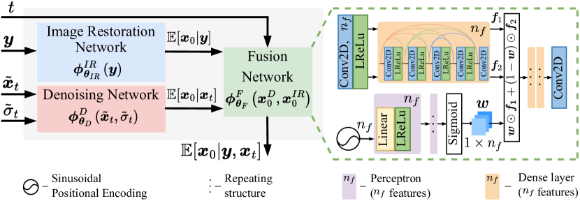
Figure 1: The proposed architecture consists of three modules: a Denoising Network $\bm{\phi}^{D}_{\bm{\theta}_{D}}\left(\tilde{\bm{x}}_{t},\tilde{\sigma}_{t}\right)$, an IR Network $\bm{\phi}^{IR}_{\bm{\theta}_{IR}}\left(\bm{y}\right)$ and a Fusion Network $\bm{\phi}^{F}_{\bm{\theta}_{F}}\left(\bm{x}_{0}^{IR},\bm{x}_{0}^{D},t\right)$. A small version of MIRNet [81] is used as the Denoising Network, while a pre-trained SwinIR [42] or BSRT [50] or FFTFormer [34] is used as the IR Network, depending on the IR task. See section 3.3 for a detailed description.

A promising direction towards IR results of high visual quality is to consider such problems within a generative framework. Several generative models have been recently proposed including Variational Autoencoders (VAEs) [33], Generative Adversarial Neural Networks (GANs) [22], Normalizing Flows (NFs) [16] and Diffusion Probabilistic Models (DPMs) [65]. Due to their impressive results in image generation, they have been further utilized to perform conditional sampling of high-quality images, with their low-quality or distorted counterparts playing the role of the conditional input [21, 38, 46, 39]. To date, DPMs appear to be the most promising framework and lead to the best results among all existing generative approaches.

Nevertheless, there are certain limitations that existing DPMs face, which hinder their wider adoption in IR tasks. In particular, inference of such models involves a sampling process that requires a large number (in the order of hundreds) of neural function evaluations (NFEs), which can be computationally very expensive, especially when considering images of high resolution. Another important limitation is that an efficient conditioning on the image measurements has yet to be proposed for DPMs in order to make them applicable to a wider range of blind IR problems. Indeed, all of the existing methods aim to learn the parameters of a single input-conditioned network for a specific blind IR task. As a result, the trained model overfits on the distribution of the condition space, and the whole model has to be retrained if we need to employ it to a different reconstruction task than the one that was initially trained for. Considering the huge amount of data and computational resources required for training a single DPM (see appendix A), such re-training becomes infeasible if at least one of the previous requirements is not satisfied.

In this work we aim to address the above issues by proposing a novel conditional diffusion network coupled with an accelerated sampling process. Specifically, our network adopts an improved conditioning strategy and is built on the foundation of existing off-the-shelf IR networks paired with a denoising module, which is applicable to a variety of reconstruction problems without requiring any re-training. Additionally, we introduce an accelerated sampling procedure that is enabled by our proposed network architecture and allows the merging of a large number of sampling steps in a single one, computed with a single NFE. Our proposed acceleration can work in tandem with accelerated sampling schemes such as DDIM [66]. To assess the performance of our network, we validate it on three challenging blind IR tasks, namely, burst joint demosaicking, denoising and super-resolution (JDD-SR), dynamic scene deblurring, and $4\times$ single image super-resolution (SISR). In all of the tested scenarios, our approach demonstrates the best perception-distortion trade-off among the state-of-the-art (SOTA) methods, while compared to other DPM-based solutions it requires a smaller number of sampling steps.

2 Related Works

Burst Image Restoration.

One of the pioneering works in multi-frame IR was introduced in [70], where a frequency-domain-based solution was proposed. Then, several MAP models with various regularization terms have been designed to cope with visual artifacts caused by operating in the frequency domain [3, 18, 63]. Using the same MAP framework, a JDD-SR method robust to noise and outliers was developed in [19]. Meanwhile, the block matching alignment algorithm of [25] was extended by [79] to obtain a robust motion model with the aid of an adaptive kernel interpolation method merging sparse pixel samples.

Advancements in deep learning have led to high-performing methods such as those in [17, 37, 4, 5, 49, 41]. The DBSR approach [4] aligns multiple input frames in the feature space utilizing an optical flow estimator (e.g. PWCNet [68]) and employs an attention-based fusion mechanism to aggregate features. In [37] a differentiable image registration module has been introduced, which exploits the aliasing effects appearing in bursts of low-resolution (LR) images. In [41] KBNet estimates blur kernels for a burst sequence to incorporate them with LR features so as to generate a better super-resolved image, while in [17] BIPNet attempts to fuse complementary information from the burst sequence with the help of generated pseudo-burst features. Another line of work effectively employs deformable convolutions for the inter-frame alignment task [49, 74, 17] and achieves SOTA results in various tasks, including burst SR.

Single Image Restoration.

Among the recent IR methods, the most successful ones are those that adopt an end-to-end supervised formulation, where a deep neural network is trained to directly map a low-quality and degraded image to a point estimate of the latent high-quality image [88, 45, 69, 83]. Consequently, in the pursuit of further improving the reconstructions and achieving a better pixel-level result, more advanced network architectures have been proposed [82, 42, 10, 34], at the cost of being more computationally heavy. While this formulation leads to SOTA fidelity (e.g. , PSNR, SSIM), the produced output is an average/median of all plausible predictions, which typically lacks high-frequency information (e.g. texture).

Generative adversarial networks (GAN) [22] have been adopted by several IR methods such as SISR [38, 73, 75] and dynamic scene deblurring  [35, 36, 85] to produce more natural and perceptually pleasing results. Although this adversarial non-reference formulation aims to push the predictions towards the manifold of natural images, it is also prone to introducing unrealistic texture and hallucinations in the output [14]. Moreover, the adversarial training process requires extra supervision as it can easily fall into a mode collapse or may diverge [2, 62].

Likelihood-based deep generative models such as NFs [47, 46], auto-regressive models [23], and VAEs [57] have also been applied to IR tasks, where one can obtain a diverse set of predictions from a learned posterior [57]. Conditioned on LR inputs, flow-based methods attempt to map high-resolution (HR) images to the latent flow-space. Although such techniques circumvent the training instability met in GANs, strong architectural constraints (e.g. network invertibility) still remain an issue.

Recently another class of methods based on a stochastic diffusion process has been introduced and demonstrated outstanding performance on various tasks that range from unconditional image generation [26, 55, 60] to image-to-image translation/restoration [39, 61, 78, 20, 60, 15, 76, 59]. DvSR proposed in [78] employs a “predict-and-refine” conditional diffusion method specifically tailored for the image deblurring task, while SRDiff [39] utilizes features of a pretrained SR model for conditional super-resolved image generation. Further, recent works in [76, 80] have considered several IR tasks (e.g. inpainting, super-resolution, colorization, etc.). In conclusion, their ability to capture complex statistics of the visual world, makes DPMs a very attractive solution that is worth being further investigated.

3 Proposed Conditional Diffusion Model

3.1 Background

Denoising Diffusion Probabilistic Models (DDPMs) [26, 65] are special cases of Hierarchical Markovian Variational Autoencoders where the dimension of the latent variables matches the dimension of the data. Starting with a sample $\bm{x}_{0}\!\in\!\mathbb{R}^{N}$, the encoding sequence $\left\{\bm{x}_{t}\right\}_{t=0}^{T}$ traverses the latent space with a diffusion process defined by a Gaussian transition probability:

$$q\left(\bm{x}_{t}|\bm{x}_{t-1}\right)\equiv\mathcal{N}\left(\bm{x}_{t};\sqrt{1-\beta_{t}}\bm{x}_{t-1},\beta_{t}\bm{I}_{N}\right).$$ (1)

The sequence $0<\beta_{1},\beta_{2},\ldots,\beta_{T}<1$ that appears in eq. 1 defines the noise scheduling for the forward process in such a way so that the latent variable at the final timestep $T$ approximates the standard Gaussian: $\bm{x}_{T}\sim\mathcal{N}\left(\bm{x}_{T};\bm{0},\bm{I}_{N}\right)$. Based on this diffusion process, it is possible to express the transition probability directly from $\bm{x}_{0}$ to $\bm{x}_{t}$ in closed form as:

$$q\left(\bm{x}_{t}|\bm{x}_{0}\right)=\mathcal{N}\left(\bm{x}_{t};\sqrt{\bar{\alpha}_{t}}\bm{x}_{0},\left(1-\bar{\alpha}_{t}\right)\bm{I}_{N}\right),$$ (2)

where $\alpha_{t}\equiv 1-\beta_{t}$ and $\bar{\alpha}_{t}\equiv\prod_{s=1}^{t}\alpha_{s}$.

The reverse process is enabled by the posterior distribution which is represented in the form:

$$p\left(\bm{x}_{t-1}|\bm{x}_{t},\bm{x}_{0}\right)=\mathcal{N}\left(\bm{x}_{t-1};\bm{\mu}_{t}\left(\bm{x}_{t},\bm{x}_{0}\right),\sigma^{2}_{t}\bm{I}_{N}\right),$$ (3)

where $\bm{\mu}_{t}\left(\bm{x}_{t},\bm{x}_{0}\right)\equiv\frac{\sqrt{\bar{\alpha}_{t-1}}\beta_{t}}{1-\bar{\alpha}_{t}}\bm{x}_{0}+\frac{\sqrt{\alpha_{t}}\left(1-\bar{\alpha}_{t-1}\right)}{1-\bar{\alpha}_{t}}\bm{x}_{t}$ and $\sigma^{2}_{t}\equiv\frac{1-\bar{\alpha}_{t-1}}{1-\bar{\alpha}_{t}}\beta_{t}$. DDPMs aim to approximate its mean by the quantity $\bm{\mu}_{\bm{\theta}}\left(\bm{x}_{t},t\right)$, which is learned from training data, and then utilize eq. 3 to perform sampling. There are different possible parameterizations of $\bm{\mu}_{t}\left(\bm{x}_{t},\bm{x}_{0}\right)$, which accordingly lead to different interpretations for the transition mean [48]. In this work, we pursue the one based on the score function $\nabla\log p\left(\bm{x}_{t}\right)$, which reads as:

$$\bm{\mu}_{t}\left(\bm{x}_{t},\bm{x}_{0}\right)=\frac{\bm{x}_{t}+\left(1-\alpha_{t}\right)\nabla\log{p\left(\bm{x}_{t}\right)}}{\sqrt{\alpha_{t}}}.$$ (4)

In this case, the reverse process defined in eq. 3 can be considered as sampling via Annealed Langevin Dynamics, in which the score function is approximated by the quantity $\bm{s}_{\bm{\theta}}\left(\bm{x}_{t},t\right)$ learned via denoising score matching [28, 72].

3.2 Conditional Score Matching

The diffusion models described above do not take into account the dependence of the sampled data on their degraded observations $\bm{y}\!\in\!\mathbb{R}^{M}$, when we are dealing with IR problems. Fortunately, the score-based models can be extended to accommodate conditional sampling by replacing the score function in eq. 4 with a conditional score function $\nabla_{\bm{x}_{t}}\log p\left(\bm{x}_{t}|\bm{y}\right)$. For non-blind IR problems, a popular approach is to decompose the conditional score function into a score function $\nabla\log p\left(\bm{x}_{t}\right)$ and a log-likelihood gradient term $\nabla_{\bm{x}_{t}}\log p\left(\bm{y}|\bm{x}_{t}\right)$ [54, 67]. This last term is directly dependent on the image formation model, which unfortunately is unknown for blind IR tasks. Therefore, most of the existing works [39, 59, 60] aim instead to learn the primal conditional score function $\nabla_{\bm{x}_{t}}\log p\left(\bm{x}_{t}|\bm{y}\right)$ via ad-hoc conditional denoising score matching. In this work, we also utilize the primal conditional score function, but we rely on its explicit form as given in the following lemma, whose proof is provided in the appendix B.

Lemma 3.1.

Let $\bm{y}\!\in\!\mathbb{R}^{M}$, $\bm{x}_{0}\!\in\!\mathbb{R}^{N}\sim p\left(\bm{x}_{0}|\bm{y}\right)$, and $\bm{x}_{t}\!\in\!\mathbb{R}^{N}$, $\bar{\alpha}_{t}\!\in\!\mathbb{R}$ are defined as in eq. 2. Then, the conditional score function is computed as:

$$\vspace{-2mm}\nabla_{\bm{x}_{t}}\log p\left(\bm{x}_{t}|\bm{y}\right)=\frac{\sqrt{\bar{\alpha}_{t}}\operatorname{\mathbb{E}}\left[\bm{x}_{0}|\bm{y},\bm{x}_{t}\right]-\bm{x}_{t}}{1-\bar{\alpha}_{t}}.$$ (5)

The above result implies that the conditional score function can be approximated by utilizing a trained joint reconstruction and denoising model. Specifically, if the augmented variable $\bm{z}_{t}=\begin{bmatrix}\bm{y}^{\mathsf{T}}&\bm{x}_{t}^{\mathsf{T}}\end{bmatrix}^{\mathsf{T}}$ represents the union of the degraded data $\bm{y}$ and the noisy data $\bm{x}_{t}$, then the conditional expected value $\operatorname{\mathbb{E}}\left[\bm{x}_{0}|\bm{z}_{t}\right]$ corresponds to the reconstructed underlying image $\bm{x}_{0}$ from the measurements $\bm{z}_{t}$.

A joint reconstruction model $\bm{\phi}_{\bm{}\theta}\left(\bm{y},\bm{x}_{t},t\right)$ can be trained by the minimization of the empirical expected pixel mean-squared error (MSE) across the samples from the training dataset $\mathcal{D}\left(\bm{x}_{0},\bm{y},\bm{x}_{t},t\right)$:

$$\min_{\bm{\theta}}\operatorname{\mathbb{E}}_{\bm{x}_{0},\bm{x}_{t},\bm{y}\sim\mathcal{D}}\lVert\bm{\phi}_{\bm{\theta}}\left(\bm{y},\bm{x}_{t},t\right)-\bm{x}_{0}\rVert^{2}_{2}=\min_{\bm{\theta}}\sum_{i}\lVert\bm{\phi}_{\bm{\theta}}\left(\bm{y}^{i},\bm{x}^{i}_{t},t\right)-\bm{x}^{i}_{0}\rVert^{2}_{2}.$$ (6)

The optimal solution is the conditional expectation $\bm{\phi}^{\textrm{MSE}}_{\bm{}\theta}\left(\bm{y},\bm{x}_{t},t\right)=\operatorname{\mathbb{E}}\left[\bm{x}_{0}|\bm{y},\bm{x}_{t}\right]$, and, thus, such a trained model can be substituted in eq. 5. This amounts to approximating the conditional score function $\nabla_{\bm{x}_{t}}\log p\left(\bm{x}_{t}|\bm{y}\right)$ with $\bm{s}_{\bm{\theta}}^{c}\left(\bm{y},\bm{x}_{t},t\right)\equiv\frac{\sqrt{\bar{\alpha}_{t}}\bm{\phi}_{\bm{}\theta}\left(\bm{y},\bm{x}_{t},t\right)-\bm{x}_{t}}{1-\bar{\alpha}_{t}}$.

3.3 Proposed Network Architecture

Our objective is to parameterize the function $\bm{\phi}_{\bm{}\theta}\left(\bm{y},\bm{x}_{t},t\right)$ in a form of a neural network (CNN) and design a specific architecture of this network. The absence of explicit knowledge about the formation model $\bm{x}_{0}\rightarrow\bm{y}$ requires the network to learn it implicitly from training data. Such an approach generally results in over-fitting, meaning that the trained model can only be employed for the task it was originally trained for [39, 78].

To overcome this problem, we initially build on the hypothesis that the conditional expectation $\operatorname{\mathbb{E}}\left[\bm{x}_{0}|\bm{y},\bm{x}_{t}\right]$ related to the conditional score function in eq. 5, can be approximated by a function of two easier to compute conditional expectations, that is

$$\operatorname{\mathbb{E}}\left[\bm{x}_{0}|\bm{y},\bm{x}_{t}\right]\approx f\left(\operatorname{\mathbb{E}}\left[\bm{x}_{0}|\bm{y}\right],\operatorname{\mathbb{E}}\left[\bm{x}_{0}|\bm{x}_{t}\right]\right).$$ (7)

Based on such an approximation, it is now possible to learn a single unconditional generative denoising model that can be applied in different reconstruction problems. Further, we note that despite the absence of a good approximation of the likelihood term, $\operatorname{\mathbb{E}}\left[\bm{x}_{0}|\bm{y}\right]$, various task-specific networks trained with a fidelity objective are readily available in the literature. Indeed, using a similar reasoning as the one provided for eq. 6, such reconstruction networks can output a good approximation of the quantity $\operatorname{\mathbb{E}}\left[\bm{x}_{0}|\bm{y}\right]$. This finally motivates us to express the joint reconstruction and denoising network $\bm{\phi}_{\bm{}\theta}\left(\bm{y},\bm{x}_{t},t\right)$ into three components (see Figure 1). Specifically, our network can be described as $\bm{\phi}^{F}_{\bm{\theta}_{F}}\left(\bm{\phi}^{IR}_{\bm{\theta}_{IR}}\left(\bm{y}\right),\bm{\phi}^{D}_{\bm{\theta}_{D}}\left(\tilde{\bm{x}}_{t},\tilde{\sigma}_{t}\right),t\right)$, where $\tilde{\bm{x}}_{t}\equiv\tfrac{\bm{x}_{t}}{\sqrt{\bar{\alpha}_{t}}}\sim\mathcal{N}\left(\bm{x}_{0},\tilde{\sigma}^{2}_{t}\bm{I}_{N}\right)$ is the noisy version of $\bm{x}_{0}$ with noise variance $\tilde{\sigma}^{2}_{t}\equiv\tfrac{1-\bar{\alpha}_{t}}{\bar{\alpha}_{t}}$ according to eq. 2, and the sub-modules $\bm{\phi}^{D}_{\bm{\theta}_{D}},\bm{\phi}^{IR}_{\bm{\theta}_{IR}},\bm{\phi}^{F}_{\bm{\theta}_{F}}$ are defined next.

IR network $\bm{\phi}^{IR}_{\bm{\theta}_{IR}}\left(\bm{y}\right)$, which is learned in a supervised manner to predict $\operatorname{\mathbb{E}}\left[\bm{x}_{0}|\bm{y}\right]$. Specifically, we employ the BSRT-Small [50] for burst JDD-SR, FFTformer [34] for dynamic scene deblurring, and SwinIR [42] for SISR. We do not train these networks but use their publicly available trained weights.

Denoising network $\bm{\phi}^{D}_{\bm{\theta}_{D}}\left(\tilde{\bm{x}}_{t},\tilde{\sigma}_{t}\right)$, which is learned in a supervised manner to predict $\operatorname{\mathbb{E}}\left[\bm{x}_{0}|\bm{x}_{t}\right]$ by denoising $\tilde{\bm{x}}_{t}$. Specifically, we employ a smaller version of MIRNet [81], which we call MIRNet-S. It is obtained by reducing the amount of RRG and MRB blocks from the original architecture to three and one, respectively. We refer to the original paper [81] for the detailed description of the blocks structure, as we use them without any modifications. Once trained, this network is reused for all considered reconstruction problems. We note that we our motivation for utilizing a smaller version of MIRNet as a Denoising module, is to approximately match the number of parameters and the computational complexity of the networks used in our framework with those of the alternative methods under study. This way we can ensure a fair evaluation and comparison among competing methods. Such strategy has allowed us to achieve direct performance comparisons under similar conditions.

Fusion network $\bm{\phi}^{F}_{\bm{\theta}_{F}}\left(\bm{x}_{0}^{IR},\bm{x}_{0}^{D},t\right)$, which predicts the conditional expectation $\operatorname{\mathbb{E}}\left[\bm{x}_{0}|\bm{y},\bm{x}_{t}\right]$. This module refines and combines the predictions of the previous two networks and is the only one that needs to be trained for each specific IR task. The fusion network accepts as inputs the image estimates $\bm{x}_{0}^{IR},\bm{x}_{0}^{D}$ and a timestep $t$. Its architecture consists of two branches. The first one involves a convolution layer with $n_{f}$ output channels followed by a single dense block [27] without batch normalization. Its purpose is to independently encode both input images into the corresponding features $\bm{f}_{1},\bm{f}_{2}$ with $n_{f}$ channels each. The second branch encodes the timestep $t$ into a vector of weights $\bm{w}\in\left(0,1\right)^{n_{f}}$ using the sinusoidal positional encoding [71], followed by a two layer perceptron and a sigmoid function as the final activation. The features $\bm{f}_{1},\bm{f}_{2}$ and the weights $\bm{w}$ are then passed to the Convex Combination Channel Attention (3CA) layer, which performs the per-channel aggregation of input features as a convex combination of the form: $\bm{w}\odot\bm{f}_{1}+\left(\bm{1}-\bm{w}\right)\odot\bm{f}_{2}$. The output of this layer is decoded by two consequent dense blocks with $n_{f}$ channels each, followed by a convolution layer which produces the final output $\operatorname{\mathbb{E}}\left[\bm{x}_{0}|\bm{y},\bm{x}_{t}\right]$. This proposed architecture results in a significantly smaller network size than those of the Denoising and IR modules. Thus we can train the fusion network fast and by using only a small amount of problem-specific training data. While we explored several basic fusion architectures, we did not delve into extensive research to ascertain the optimal design. Our proposed fusion module serves as a proof of concept, validating our framework and demonstrating its potential for performance enhancement. A comprehensive investigation into optimal fusion architectures remains a promising area for future research.

Such a modular overall architecture allows us to capitalize on the existing SOTA non-blind denoising and blind IR networks, while it also allows us to easily replace any of these networks when better ones become available in the future. As we describe next, another important advantage of our proposed pipeline, is that it allows us to achieve a significant acceleration for the sampling process without incurring any loss of reconstruction quality.

3.4 Proposed Accelerated Sampling

According to eq. 3, our conditional denoiser should be evaluated for all timesteps $t=\overline{T,...,0}$, which leads to a total of $T$ NFEs. We note that by construction, for the forward process it holds that $\bm{x}_{T}\sim\mathcal{N}\left(\bm{0},\bm{I}_{N}\right)$. This means that in the beginning of sampling, the latent variable $\bm{x}_{T}$ does not contain any information about $\bm{x}_{0}$. It is also reasonable to expect that a similar lack of information about $\bm{x}_{0}$ exists for a number of steps prior to $T$. Specifically, for those steps we expect that the quantity $\operatorname{\mathbb{E}}\left[\bm{x}_{0}|\bm{y},\bm{x}_{t}\right]$ is heavily influenced by $\operatorname{\mathbb{E}}\left[\bm{x}_{0}|\bm{y}\right]$, while the contribution of $\operatorname{\mathbb{E}}\left[\bm{x}_{0}|\bm{x}_{t}\right]$ is not significant enough. A theoretical justification for this argument is provided in appendix C.

Based on the above reasoning, we select a timestep $\tau$ such that for the first $T-\tau$ reverse steps we use the following approximation: $\operatorname{\mathbb{E}}\left[\bm{x}_{0}|\bm{y},\bm{x}_{t}\right]\approx\operatorname{\mathbb{E}}\left[\bm{x}_{0}|\bm{y}\right]=\bm{\phi}^{IR}_{\bm{\theta}_{IR}}\left(\bm{y}\right)$. This is achieved by disabling the lower branch of our proposed conditional score matching network, namely the Denoising $\bm{\phi}^{D}_{\bm{\theta}_{D}}\left(\tilde{\bm{x}}_{t},\tilde{\sigma}_{t}\right)$ and Fusion $\bm{\phi}^{F}_{\bm{\theta}_{F}}\left(\bm{x}_{0}^{IR},\bm{x}_{0}^{D}\right)$ modules (Figure 1). Our strategy can be further supported by the recent study in [12], where it has been demonstrated that the image sampling via DPMs could be divided into stages depending on the reverse process timesteps. In this spirit we activate the Denoising and Fusion modules at a timestep $\tau$ that is selected experimentally for the particular IR task of interest. Our results clearly indicate that the reconstruction result is going to be exactly the same whether we utilize the multi-step reverse diffusion process or the proposed one-step process that is described in Lemma 3.2.

Indeed, since the quantity $\operatorname{\mathbb{E}}\left[\bm{x}_{0}|\bm{y}\right]$ is predicted by the IR network, which does not depend on the reverse diffusion parameters, $\bm{\phi}^{IR}_{\bm{\theta}_{IR}}\left(\bm{y}\right)$ needs to be evaluated only once and its output can be re-used throughout the whole iterative sampling procedure. Expanding more on this idea, we show in Lemma 3.2 that it is possible to omit entirely the first $T-\tau$ reverse diffusion steps and instead perform a single step directly from $T$ to $\tau$ with a procedure very similar to the one obtained for the diffusion process in eq. 2 from eq. 1. We provide the derivation in appendix D.

Figure 2: Forward and reverse diffusion process. Blue solid arrows: transitions at the forward pass with sampling distribution from eq. 1. Dashed arrow: cumulative transition probability from eq. 2. Black solid arrows: transitions at the backward pass with the sampling distribution from eq. 3. Red solid arrow: closed-form cumulative transition probability from eq. 8 representing our accelerated sampling.

Table 1: Performance evaluation on the task of Burst JDD-SR. We highlight the overall best for each metric.

Methods	PSNR$\uparrow$	SSIM$\uparrow$	LPIPS$\downarrow$	TOPIQΔ$\downarrow$	NFE $\downarrow$	Params$\downarrow$
Target	$\infty$	1	0	0	N/A	N/A
DBSR	31.98	0.891	0.198	0.10	N/A	13.0M
DeepRep	34.66	0.927	0.136	0.07	N/A	12.1M
EBSR	36.05	0.940	0.111	0.15	N/A	26.0M
BIPNet	34.86	0.934	0.112	0.03	N/A	6.7M
BSRT-Small	35.91	0.940	0.109	0.12	N/A	4.9M
BSRT-Large	36.98	0.947	0.095	0.16	N/A	20.7M
Ours	35.53	0.933	0.084	0.02	6	21.6M

Lemma 3.2.

The transition probability defined in eq. 3 for a single reverse step, can be extended to $k$ reverse steps starting from $\bm{x}_{t}$ as:

$$p(\bm{x}_{t-k}|\bm{x}_{t},\bm{x}_{0})=\mathcal{N}\left(\bm{x}_{t-k};\bm{\mu}_{t,k}\left(\bm{x}_{t},\bm{x}_{0}\right),{\sigma^{2}_{t,k}}\bm{I}_{N}\right),$$ (8)

where

$$\bm{\mu}_{t,k}\left(\bm{x}_{t},\bm{x}_{0}\right)=\sum_{i=0}^{k-1}\Gamma_{t-i-1}^{t-k+1}\gamma_{t-i}\bm{x}_{0}+\Gamma_{t}^{t-k+1}\bm{x}_{t}\,\,\,\mbox{and}\,\,\,\sigma^{2}_{t,k}=\sum_{i=0}^{k-1}\left(\Gamma_{t-i-1}^{t-k+1}\right)^{2}\sigma_{t-i}^{2}.$$ (9)

In the above equations we make use of the following notation:

$$\gamma_{t}=\frac{\sqrt{\bar{\alpha}_{t-1}}\beta_{t}}{1-\bar{\alpha}_{t}}\,\,\,\mbox{and}\,\,\,\Gamma_{i}^{j}\equiv\begin{cases}\sqrt{\prod_{n=j}^{i}\alpha_{n}}\frac{1-\bar{\alpha}_{j-1}}{1-\bar{\alpha}_{i}}&\text{for }i\geq j\\ 1&\text{for }i<j\end{cases}$$ (10)

Since for the first $T-\tau$ steps $\bm{x}_{0}$ is approximated by the quantity $\operatorname{\mathbb{E}}\left[\bm{x}_{0}|\bm{y}\right]$, which is independent of the timestep $t$, we utilize eq. 8 to directly sample $\bm{x}_{\tau}$ as

$$\bm{x}_{\tau} \sim p\left(\bm{x}_{\tau}|\bm{x}_{T},\operatorname{\mathbb{E}}\left[\bm{x}_{0}|\bm{y}\right]\right)=\mathcal{N}\left(\bm{x}_{\tau};\bm{\mu}_{T,T-\tau}\left(\bm{x}_{T},\operatorname{\mathbb{E}}\left[\bm{x}_{0}|\bm{y}\right]\right),\sigma^{2}_{T,T-\tau}\bm{I}\right).\vspace{-1mm}$$ (11)

This allows us to reduce the NFEs from $T\!+\!1$ to $\tau\!+\!1$, meaning that the required evaluations of Denoising + Fusion networks is reduced from $T$ to $\tau$. In both cases, we additionally count a single evaluation of the IR network. We depict our acceleration strategy with a red arrow in Figure 2. Finally, in practice we use $\tau=\tfrac{T}{200}$ for burst JDD-SR and dynamic scene deblurring, and $\tau=\tfrac{T}{4}$ for SISR, effectively reducing the NFEs by two orders of magnitude and a factor of four, respectively.

The proposed acceleration procedure can be also interpreted as starting the sampling from step $\tau$ of the latent space using a non-standard Gaussian distribution as defined in eq. 11, instead of starting from step $T$ and using a standard Gaussian sample $\bm{x}_{T}\sim\mathcal{N}\left(\bm{0},\bm{I}_{N}\right)$. We note, that a similar idea was explored in [13, 52], where it was proposed to start the sampling from an observation that has been passed through a predefined number of forward diffusion steps. In our case the starting point for sampling is obtained via the approximated reverse process, which as a consequence of Lemma 3.2 does not alter the final reconstruction result. In another words, if we approximate $\bm{x}_{0}$ with $\mathbb{E}\left[\bm{x}_{0}|\bm{y}\right]$, then the reconstruction result will be the same both for the multi-step reverse diffusion process and the proposed one-step process. Moreover, it is easy to show that our strategy generalizes the one proposed in [13, 52], as it leads to the same starting point if we make the following specific choices: $\bm{x}_{T}\sim\mathcal{N}\left(\sqrt{\bar{\alpha}_{T}}\mathbb{E}\left[\bm{x}_{0}|\bm{y}\right],\left(1-\bar{\alpha}_{T}\right)\bm{I}\right)$ and $\sigma_{t}^{2}=\frac{1-\bar{\alpha}_{t-1}}{1-\bar{\alpha}_{t}}\beta_{t}$. In practice $\bar{\alpha}_{T}\approx 0$, so the first condition holds almost exactly. The second condition represents the particular choice of the noise variance used in the reverse process, with several existing parametrizations [26, 55]. Our method is compatible with all of them and leads to different distributions for the starting point. In all our experiments we use the parametrization $\sigma_{t}^{2}=\beta_{t}$ from [26]. More detailed conceptual and technical differences along with experimental results are provided in appendix E.

Furthermore, our acceleration strategy is complimentary to other sampling acceleration techniques [66, 31]. To demonstrate this, we utilize the DDIM [66] sampling to further reduce the NFEs by a factor of five for the SISR task. As a result, the reverse diffusion process used for this problem requires $\tfrac{T}{20}+1$ NFEs in total.

4 Experimental Results

We evaluate our method on four public datasets across a range of tasks, namely burst JDD-SR, dynamic scene deblurring, and SISR. Below we describe our specific architecture and design choices related to all utilized modules.

Training.

Our training procedure consists of two stages. We first employ a diverse, yet small DF2K (combination of DIV2K [1] and Flickr2K [45]) dataset to train a Denoising Module for Gaussian denoising in the sRGB domain with input noise levels ranging in $[0,244.3]$. These noise levels corresponds to timesteps in the range of $[0,250]$ for the diffusion process with $T=1000$. We use the original training procedure of MIRNet [81] to learn the parameters of our MIRNet-S architecture. At the second stage we train our Fusion Modules with $n_{f}=64$ for each IR task and the corresponding pre-trained off-the-shelf IR network. It is worth noting, that at this stage the parameters of Denoising and IR modules are kept frozen and only the Fusion Module is trained. Specifically, we train it for $300k$ iterations with a learning rate of $10^{-4}\times 0.99$ it/1000, batch size of 128, and crop size of $256\times 256$. To train our Fusion networks we use datasets that are common among our main competitors, specifically the ZurichRAW2RGB [29] dataset for burst JDD-SR, GoPro [53] for dynamic scene deblurring and DIV2K [1] for $4\times$ SISR. For burst JDD-SR the Fusion network is trained in the sRGB domain. All the networks are trained using the Ascend 910 AI accelerators [44]. To make our results reproducible, we provide a full description of the training procedure in appendix H.

Inference.

For each IR task we use the procedure described in section 3.4 to obtain the reconstructed images with $T=1000$. To demonstrate the effectiveness of our approach, for each problem of interest except for burst JDD-SR we need half of the NFEs compared to the diffusion-based competitor that uses the least number of sampling steps. Specifically, for dynamic scene deblurring we use $\tau=5$, resulting in $200\times$ acceleration achieved solely by our proposed sampling strategy. This amounts to $6$ NFEs when counting the additional IR network evaluation performed to skip the first $T-\tau=995$ steps using eq. 8. For SISR we select $\tau=250$, which results in $4\times$ acceleration using our sampling procedure. In order to demonstrate how it can be complemented by other proposed acceleration strategies, for the final $\tau=250$ steps we achieve $5\times$ step reduction by employing DDIM sampling [66]. The combination of both acceleration strategies results in $20\times$ step reduction and $51$ NFEs overall. Applying the DDIM acceleration technique on top of our proposed one-step strategy leads to an insignificant quantitative/qualitative difference (see appendix G) compared to our original scheme. Since for the burst JDD-SR problem no diffusion-based methods have yet been proposed, we use the same setting as for the dynamic scene deblurring problem, as it requires the smallest NFEs. In all our experiments we use the linear scheduling of the diffusion process variances $\beta_{t}\in\left[2\times 10^{-2},10^{-4}\right]$ defined in eq. 1.

Evaluation.

For the burst JDD-SR evaluation we use the SyntheticBurst test set [4], consisting of 300 synthetically pre-generated raw burst sequences. Each sequence contains 14 noisy raw LR images with handshake motion, whose corresponding targets have a resolution of $320\times 320$. Since our networks are trained on sRGB images, the outputs of all methods are converted to the sRGB space prior to comparison. For dynamic scene deblurring we evaluate on the GoPro test [53] and HIDE [64] benchmarks, which contain 1111 and 2025 images of 720p resolution, respectively. For $4\times$ SISR we use the DIV2K validation dataset [1] consisting of 100 images of 2K resolution.

For the quantitative evaluation of the reconstruction quality we rely on the widely used fidelity metrics PSNR and SSIM [77], and the reference-based perceptual metric LPIPS [86]. Moreover, we also utilize the non-reference image quality assessment (NR-IQA) metric TOPIQ [8] and report the absolute distance between the output and the target scores, which we indicate as TOPIQ_Δ.

Table 2: Performance evaluation on the GoPro and HIDE test sets for dynamic scene deblurring. ^† indicates that public implementation is unavailable and the scores are copied from the authors’ paper. We highlight the overall best for each metric, and the best among perceptual-oriented methods.

Methods	GoPro				HIDE				NFE $\downarrow$	Params $\downarrow$
	PSNR$\uparrow$	SSIM$\uparrow$	LPIPS$\downarrow$	TOPIQΔ$\downarrow$	PSNR$\uparrow$	SSIM$\uparrow$	LPIPS$\downarrow$	TOPIQΔ$\downarrow$
Target	$\infty$	1	0	0	$\infty$	1	0	0	N/A	N/A
HINet	32.77	0.960	0.088	0.033	30.33	0.932	0.120	0.044	N/A	88.6M
MPRNet	32.66	0.959	0.089	0.027	30.96	0.939	0.114	0.059	N/A	20.1M
MIMO-UNet+	32.44	0.957	0.091	0.034	29.99	0.930	0.124	0.028	N/A	16.1M
NAFNet	33.71	0.967	0.078	0.017	31.32	0.943	0.103	0.024	N/A	67.9M
Restormer	32.90	0.961	0.084	0.018	31.20	0.942	0.109	0.048	N/A	26.1M
FFTFormer	34.21	0.969	0.071	0.012	31.62	0.946	0.096	0.006	N/A	16.6M
Perceptual-oriented Methods
DeblurGANv2	29.08	0.918	0.117	0.025	27.51	0.885	0.159	0.065	N/A	60.9M
DvSR†	31.66	0.948	0.059	-	29.77	0.922	0.089	-	500	26.1M
icDPM†	31.19	0.943	0.057	-	29.14	0.910	0.088	-	500	52.0M
InDi†	31.49	0.946	0.058	-	-				10	27.7M
Ours	33.72	0.963	0.053	0.011	31.32	0.937	0.087	0.002	6	33.2M

4.1 Results

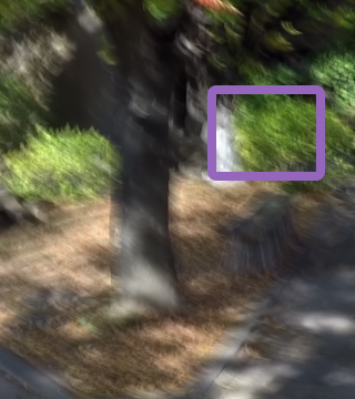
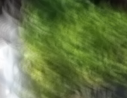
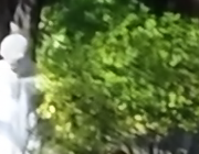
	Input: 0.424	HINet: 0.127	Restormer: 0.136	DeblurGANv2: 0.171	InDI: 0.080
	Target	NAFNet: 0.083	FFTFormer: 0.059	DvSR: 0.072	Ours: 0.059

Figure 3: Visual comparisons on the GoPro test set for the task of dynamic scene deblurring (best viewed by zooming in). Every output image is accompanied by its LPIPS value.

Burst JDD-SR.

In Table 1 we compare our proposed pipeline with existing methods, namely DBSR [4], DeepRep [5], and the current SOTA methods, namely BIPNet [17], BSRT-Small [50], BSRT-Large [50], and EBSR [49]. Our method demonstrates SOTA performance across the perceptual metrics while maintaining competitive PSNR and SSIM scores compared to existing methods. Thus, our method reconstructs images that are closer to the target based on the human perception while maintaining a high level of fidelity. We refer to figures in the appendix M for a qualitative visual assessment. Furthermore, we notice an improvement in terms of visual quality and perceptual metrics compared to BSRT-Small, which we use as the IR module of choice in our framework. This indicates that our approach preserves the fidelity of the IR model outputs, while enhancing their perceptual quality by running few reverse diffusion steps. It is worth noting that for this case, where a burst of raw images serves as input, we use the exact same denoising network that was trained on sRGB images and which we later deploy to all considered single-input IR tasks. This highlights the generalization ability of our approach not only to different IR problems but also to different input formats. Note that AFCNet [51], LKR [37], and Burstormer [17] are not included in our comparisons due to the absence of a publicly available implementation (or trained network parameters). Finally, the comparison with SOTA EBSR and BSRT shows that our DP-IR reconstructions compares favorably in terms of visual quality, while not lacking significantly in terms of fidelity.

Dynamic Scene Deblurring.

Table 2 show quantitative results on the GoPro [53] and HIDE [64] datasets, respectively. We compare our approach with the SOTA reconstruction-based methods: NAFNet [59], FFTFormer [34] and diffusion-based methods: DvSR [78], InDI [15], and icDPM [59]. Our framework outperforms all competing methods across the perceptual metrics and demonstrates the best perception-distortion (P-D) trade-off among all perceptual-based methods. Moreover, our DP-IR uses twice less number of reverse steps (NFE=5) compared to the state-of-the-art InDI and still achieves better perceptual quality (e.g. LPIPS) and is more consistent with the ground-truth (+2.22dB in PSNR). Despite the fact that our fusion module is trained only on the GoPro dataset, the gains in perceptual quality do transfer over the HIDE test images, providing SOTA scores for the perceptual metrics. Also, among perceptual-oriented methods, DP-IR outperforms the closest competitor DvSR by 1.55dB in terms of PSNR. Visual comparisons of our method and the SOTA deblurring models: NAFNet, FFTFormer, DvSR, and InDI is depicted in Figure 3. From these results we observe that our model shows a noticeable improvement in perceptual quality. Moreover, we have performed a computational cost analysis for the diffusion-based models and significantly outperformed existing methods from $\sim$2 to 100 times (see appendix F).

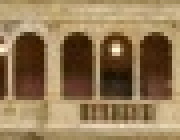
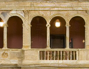
	Input: 0.341	SwinIR: 0.123	HCFlow: 0.109	ESRGAN: 0.092	InDI: 0.078
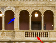
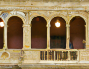
	Target	HAT: 0.128	LDM: 0.140	SRDiff: 0.122	Ours: 0.077

Figure 4: Visual comparisons on the DIV2K validation set for the task of $4\times$ bicubic super-resolution (best viewed by zooming in). Every output image is accompanied by its LPIPS value.

Table 3: Performance evaluation on the DIV2K validation set for $4\times$ SISR. We highlight the overall best for each metric, and the best among perceptual-oriented methods.

Methods	PSNR$\uparrow$	SSIM$\uparrow$	LPIPS$\downarrow$	TOPIQΔ$\downarrow$	NFE $\downarrow$	Params$\downarrow$
Target	$\infty$	1	0	0	N/A	N/A
SRResNet	29.07	0.824	0.266	0.046	N/A	1.5M
RRDB	29.48	0.834	0.254	0.038	N/A	16.7M
SwinIR	29.63	0.837	0.248	0.030	N/A	11.9M
LIIF	29.30	0.830	0.258	0.046	N/A	22.3M
HAT	29.75	0.840	0.245	0.035	N/A	20.6M
Perceptual-oriented Methods
ESRGAN	26.64	0.758	0.115	0.014	N/A	16.7M
HCFlow	27.02	0.766	0.124	0.021	N/A	23.2M
SwinIR-GAN	24.88	0.734	0.222	0.115	N/A	11.9M
LDM	23.30	0.697	0.218	0.019	100	169.0M
SRDiff	27.14	0.773	0.129	0.008	100	23.6M
InDI	26.45	0.741	0.136	0.009	100	62.3M
IDM	27.35	0.782	0.147	0.008	2000	116.6M
Ours	28.12	0.793	0.140	0.002	51	28.5M

Table 4: Ablation on various denoiser and IR networks on DIV2K validation for $4\times$ SISR.

Denoiser	IR Network	PSNR$\uparrow$	SSIM$\uparrow$	LPIPS$\downarrow$	TOPIQΔ$\downarrow$
Target		inf	1	0	0
UDP	RRDB	27.93	0.777	0.149	0.006
MIRNet-S	RRDB	28.12	0.795	0.150	0.014
MIRNet-S	SwinIR	28.12	0.793	0.140	0.002

Table 5: Ablation on various fusion networks on DIV2K validation for $4\times$ SR task

Fusion Module	PSNR$\uparrow$	SSIM$\uparrow$	LPIPS$\downarrow$	Params
TDWA	27.26	0.751	0.266	8385
L-DWT	29.27	0.818	0.233	30.0M
U-Net	28.19	0.785	0.141	31.0M
Proposed Fusion	27.93	0.777	0.149	0.7M

Table 6: Perception-Distortion trade-off on DIV2K validation for $4\times$ SISR.

Timestep, $\tau$	50	100	150	200	250	300	350
PSNR $\uparrow$	28.77	28.46	28.24	28.06	27.93	27.81	27.71
LPIPS$\downarrow$	0.170	0.161	0.155	0.152	0.149	0.147	0.146

Super-Resolution.

We compare our method with reconstruction-based [38, 73, 42, 11, 10], GAN-based [73, 87, 42], NF-based [43] models, and DPMs [60, 39, 15, 20]. Table 6 summarizes the quantitative results on the DIV2K validation set. Our solution produces the best fidelity scores among all six perceptual-based methods and the best TOPIQ perceptual metric among all competing methods. The visual comparison in Figure 4 reveals that our framework produces super-resolved images that exhibit more refined structures and fine-grained details. Additional examples for all reported IR tasks are provided in appendix M.

5 Ablation Studies

Modular Approach.

One of the main benefits of our framework is its ability to capitalize on the performance of existing restoration networks at a relatively low additional computational cost. To showcase this, we conduct an experiment on the task of $4\times$ SISR using two different denoising architectures, namely UDP [7] and MIRNet-S [81], and two IR architectures, namely RRDB [1] and SwinIR [42]. UDP is trained with the same settings as MIRNet-S and the fusion module is retrained for each of the three cases. From Table 6, we observe that the same IR network combined with a better denoising module, leads to better fidelity (see PSNR, SSIM). A same trend, but for perceptual metrics is observed if one upgrades the IR module from RRDB to the SwinIR and keeps the same denoising module. This clearly indicates that one can achieve better results by employing either a more powerful denoiser or IR module, without the need to fully retrain the entire score estimator as is the common practice followed in most of the existing methods (e.g. LDM, SRDiff, DvSR, etc. ).

Fusion Strategies.

In this study we use the UDP denoiser and the RRDB network from Table 6 and study several different fusion approaches, namely the Time-dependent Weighted Averaging (TDWA), Learnable Discrete Wavelet Transform (L-DWT), our proposed Fusion network, and U-Net with time embeddings [56]. TDWA consists of sinusoidal positional encoding followed by a three-layer MLP, which predicts the weights for the timestep $t$.

Those weights are then passed to the 3CA layer (section 3.3) together with the outputs from the denoiser and IR modules to perform the fusion in the image space. In contrast, L-DWT directly learns weights for each scale and channel of a 3-level Haar DWT [24]. L-DWT has only 30 trainable parameters, which needs significantly less training time and data. Table 6 indicates that, as expected, a more powerful fusion module leads to better perceptual and reconstruction quality. Overall, we see that the proposed Fusion network shows a better balance between the reconstruction, visual quality and the computational cost.

Perception-Distortion Trade-off.

By varying the timestep $\tau$, when the denoiser and fusion modules are activated, one can favor the perceptual quality over the reconstruction fidelity (see Table 6). Here, we use the same UDP denoiser and RRDB as the IR module and experiment on the DIV2K [1] validation for the task of $4\times$ SISR. Table 6 shows that the denoiser can operate on $\tau>250$, which corresponds to a wider noise range than the one the denoiser is initially trained for. Furthermore, we observe the same perception-distortion trade-off for dynamic scene deblurring task (see Appendix Table 13)

Limitations

Our empirical findings highlight that the optimal selection of $\tau$ is intrinsically linked to the nature of the reconstruction problem, particularly the output quality of the IR Network. While we have experimentally identified optimal parameters for each test dataset in this study, we posit that a more refined approach would involve tailoring the acceleration parameters on an individual sample basis. However, the absence of a dependable methodology for assessing the quality of the IR and Denoising Networks’ outputs at specific diffusion process timesteps – especially in the absence of ground truth data – constitutes a considerable challenge. This underscores a compelling avenue for future inquiry into adaptive optimization of acceleration parameters.

Furthermore, a notable constraint of our approach is its reliance on the efficacy of the employed Denoising and IR modules. As such, for novel image restoration tasks where a pre-trained IR network is unavailable, our framework might be inapplicable. Additionally, for imaging modalities (e.g. medical imaging) lacking a trained score-matching network (denoising module), it is imperative to either fine-tune an existing module or undertake comprehensive re-training with appropriate image datasets.

6 Conclusion

We present a modular conditional diffusion probabilistic framework for IR problems along with a sampling acceleration strategy that achieves a significant speed-up during the inference stage. Our framework achieves SOTA results both quantitatively and visually on the tasks of burst JDD-SR, dynamic scene deblurring, and $4\times$ SISR without the need for re-training on a large pool of data and significant computational cost. This is mainly accomplished by utilizing pretrained models and only training a relatively small fusion module. While in this work we have not exhaustively considered all blind IR problems, we hope that our results can serve as a positive indication that the perceptual quality of the reconstructed outputs can improve significantly at the cost of only several additional NFEs, making possible a wider adoption of DPMs for IR applications even when there are tight requirements on computational complexity. Our ablation studies indicate that a variety of pretrained networks can be used with our method and further improvements on the results can be achieved by utilizing better denoising, IR, and fusion modules.

Appendix A Conditional DPM Training Requirements

To the best of our knowledge, all diffusion-based approaches that have been proposed in the literature to deal with image restoration tasks, require the training of far larger conditional backbone networks ($\sim$10-100M params). This turns out to be significantly more challenging both in terms of necessary training data and computational resources. To showcase this, we provide an indicative example below. If we adopt the existing diffusion-based SISR baselines and train them for a completely different restoration problem, by following the original authors’ training strategies it turns out that the computational and data requirements are significantly higher than those of our method.

Table 7: Comparison of the proposed approach against existing DPM methods for SISR task in terms of training dataset requirements and training parameters.

Method	Params required	Data required
Ours	$1$x	$1$x
SRDiff	$\sim 34$x	$\sim 4$x
LDM	$\sim 240$x	$\sim 1000$x
InDI	$\sim 89$x	$\sim 1$x
IDM	$\sim 167$x	$\sim 1$x

Based on these data, we can safely state that our strategy provides a reasonable trade-off between the required training complexity and the competitive performance of our method to a variety of blind inverse problems.

Appendix B Proof of Lemma 3.1

To derive the conditional score function, we first express the conditional probability $p\left(\bm{x}_{t}|\bm{y}\right)$ as:

$$p\left(\bm{x}_{t}|\bm{y}\right)=\int p\left(\bm{x}_{t},\bm{x}_{0}|\bm{y}\right)\,d\bm{x}_{0}=\int p\left(\bm{x}_{t}|\bm{y},\bm{x}_{0}\right)p\left(\bm{x}_{0}|\bm{y}\right)\,d\bm{x}_{0}=\int q\left(\bm{x}_{t}|\bm{x}_{0}\right)p\left(\bm{x}_{0}|\bm{y}\right)\,d\bm{x}_{0},$$ (12)

where we used the fact that $\bm{x}_{t}$ is conditionally independent of $\bm{y}$ and according to eq. 2 it holds $p\left(\bm{x}_{t}|\bm{y},\bm{x}_{0}\right)=q\left(\bm{x}_{t}|\bm{x}_{0}\right)$. Differentiating both sides of eq. 12 with respect to (w.r.t.) $\bm{x}_{t}$ we get:

$$\nabla_{\bm{x}_{t}}p\left(\bm{x}_{t}|\bm{y}\right)=\int p\left(\bm{x}_{0}|\bm{y}\right)\nabla_{\bm{x}_{t}}q\left(\bm{x}_{t}|\bm{x}_{0}\right)\,d\bm{x}_{0}.$$ (13)

Based on the definition of $q\left(\bm{x}_{t}|\bm{x}_{0}\right)$ in eq. 2, it also holds that: $\nabla_{\bm{x}_{t}}q\left(\bm{x}_{t}|\bm{x}_{0}\right)=-q\left(\bm{x}_{t}|\bm{x}_{0}\right)\frac{\bm{x}_{t}-\sqrt{\bar{\alpha}_{t}}\bm{x}_{0}}{1-\bar{\alpha}_{t}}$. Substituting this result back to eq. 13, we get:

$$\nabla_{\bm{x}_{t}}p\left(\bm{x}_{t}|\bm{y}\right) =\frac{\sqrt{\bar{\alpha}_{t}}}{1-\bar{\alpha}_{t}}\int\bm{x}_{0}q\left(\bm{x}_{t}|\bm{x}_{0}\right)p\left(\bm{x}_{0}|\bm{y}\right)\,d\bm{x}_{0}-\frac{\bm{x}_{t}}{1-\bar{\alpha}_{t}}\overbrace{\int q\left(\bm{x}_{t}|\bm{x}_{0}\right)p\left(\bm{x}_{0}|\bm{y}\right)\,d\bm{x}_{0}}^{p\left(\bm{x}_{t}|\bm{y}\right)}.$$ (14)

Next, if we divide both sides in eq. 13 with $p\left(\bm{x}_{t}|\bm{y}\right)$ and use that $\nabla_{\bm{x}_{t}}\log{p\left(\bm{x}_{t}|\bm{y}\right)}=\frac{\nabla_{\bm{x}_{t}}p\left(\bm{x}_{t}|\bm{y}\right)}{p\left(\bm{x}_{t}|\bm{y}\right)}$, we get:

$$\nabla_{\bm{x}_{t}}\log{p\left(\bm{x}_{t}|\bm{y}\right)}=\frac{1}{\left(1-\bar{\alpha}_{t}\right)}\left(\sqrt{\bar{\alpha}_{t}}\int\bm{x}_{0}\frac{q\left(\bm{x}_{t}|\bm{x}_{0}\right)p\left(\bm{x}_{0}|\bm{y}\right)}{p\left(\bm{x}_{t}|\bm{y}\right)}\,d\bm{x}_{0}-\bm{x}_{t}\right).$$ (15)

We can further express the integral in eq. 15 as follows:

$$\int\bm{x}_{0}\frac{q\left(\bm{x}_{t}|\bm{x}_{0}\right)p\left(\bm{x}_{0}|\bm{y}\right)}{p\left(\bm{x}_{t}|\bm{y}\right)}\,d\bm{x}_{0}=\int\bm{x}_{0}\frac{q\left(\bm{x}_{t}|\bm{x}_{0}\right)p\left(\bm{x}_{0}|\bm{y}\right)p\left(\bm{y}\right)}{p\left(\bm{x}_{t}|\bm{y}\right)p\left(\bm{y}\right)}\,d\bm{x}_{0}=\int\bm{x}_{0}\frac{p\left(\bm{x}_{t}|\bm{x}_{0},\bm{y}\right)p\left(\bm{x}_{0},\bm{y}\right)}{p\left(\bm{x}_{t},\bm{y}\right)}\,d\bm{x}_{0}$$

$$= \int\bm{x}_{0}\frac{p\left(\bm{x}_{t},\bm{x}_{0},\bm{y}\right)}{p\left(\bm{x}_{t},\bm{y}\right)}\,d\bm{x}_{0}=\int\bm{x}_{0}p\left(\bm{x}_{0}|\bm{y},\bm{x}_{t}\right)\,d\bm{x}_{0}=\operatorname{\mathbb{E}}\left[\bm{x}_{0}|\bm{y},\bm{x}_{t}\right].$$

Substituting this result in eq. 15 finally leads us to the result of the lemma: $\nabla_{\bm{x}_{t}}p\left(\bm{x}_{t}|\bm{y}\right)=\frac{\sqrt{\bar{\alpha}_{t}}\operatorname{\mathbb{E}}\left[\bm{x}_{0}|\bm{y},\bm{x}_{t}\right]-\bm{x}_{t}}{1-\bar{\alpha}_{t}}$.

Appendix C Theoretical Justification of the Conditional Expectation Approximation

By construction, for the forward process from eq. 1 it holds that $\bm{x}_{T}\sim\mathcal{N}\left(\bm{0},\bm{I}_{N}\right)$ when $T\rightarrow\infty$, which means that in the beginning of reverse sampling, the latent variable $\bm{x}_{T}$ does not contain any information about $\bm{x}_{0}$. Below we provide a theoretical result that can serve as an indication that during the sampling process and up to some timestep $\tau$, we can use an approximation of $\operatorname{\mathbb{E}}\left[\bm{x}_{0}|\bm{y},\bm{x}_{t}\right]\approx\operatorname{\mathbb{E}}\left[\bm{x}_{0}|\bm{y}\right]$, given that the contribution of $\operatorname{\mathbb{E}}\left[\bm{x}_{0}|\bm{x}_{t}\right]$ is not significant enough. This is achieved by disabling the lower branch of our proposed conditional score matching network, which includes the Denoising $\bm{\phi}^{D}_{\bm{\theta}_{D}}\left(\tilde{\bm{x}}_{t},\tilde{\sigma}_{t}\right)$ and Fusion $\bm{\phi}^{F}_{\bm{\theta}_{F}}\left(\bm{x}_{0}^{IR},\bm{x}_{0}^{D}\right)$ modules (Figure 1). A formal theoretical analysis is available under the following simplifications:

• The observation model is linear: $\bm{y}=\bm{A}\bm{x}_{0}+\bm{n}$.

• Denoising Network is an identity transformation: $\bm{\phi}^{D}_{\bm{\theta}_{D}}\left(\tilde{\bm{x}}_{t},\tilde{\sigma}_{t}\right)\equiv\tilde{\bm{x}}_{t}$.

• Image Restoration Network is a back-projection: $\bm{\phi}^{IR}_{\bm{\theta}_{IR}}\left(\bm{y}\right)\equiv\bm{A}^{T}\bm{y}$

• Fusion Network is a convex combination in a spatial domain: $\bm{\phi}^{F}_{\bm{\theta}_{F}}\left(\bm{x}_{0}^{IR},\bm{x}_{0}^{D},t\right)\equiv w\bm{x}_{0}^{IR}+(1-w)\bm{x}_{0}^{D}$.

• Diffusion process approaches the continuous-time regime: $T\rightarrow\infty$.

Our theoretical result is provided in the form of the following proposition.

Proposition C.1.

Let $\bm{y}\in\mathbb{R}^{M}$ be the measurements obtained according to the following observation model: $\bm{y}=\bm{A}\bm{x_{0}}+\bm{n}$, where $\bm{A}\in\mathbb{R}^{M\times N},\lVert\bm{A}\rVert_{2}\leq 1$ and $\bm{n}\sim\mathcal{N}\left(\bm{0},\sigma_{\bm{y}}\bm{I}_{M}\right),\sigma_{\bm{y}}\leq 1$. Then, for any given $\bm{A}$,$\sigma_{\bm{y}}$,$\bm{x}_{0}\in\mathbb{R}^{N}$, and any fixed $w\in(0,1)$, there exists a timestep $\tau$, such that for all $t>\tau$ the back-projected signal $\bm{A}^{T}\bm{y}$ approximates $\bm{x}_{0}$ better than the convex combination $w\bm{A}^{T}\bm{y}+(1-w)\tilde{\bm{x}}_{t}$ in the following sense:

$$\mathbb{E}_{\bm{y}|\bm{x}_{0}}\lVert\bm{x}_{0}-\bm{A}^{T}\bm{y}\rVert_{2}^{2}\leq\mathbb{E}_{\bm{y},\bm{x}_{t}|\bm{x}_{0}}\lVert\bm{x}_{0}-\left(w\bm{A}^{T}\bm{y}+(1-w)\tilde{\bm{x}}_{t}\right)\rVert_{2}^{2},$$ (16)

where $\tilde{\bm{x}}_{t}\sim\mathcal{N}\left(\bm{x}_{0},\tilde{\sigma}^{2}_{t}\bm{I}_{N}\right),\tilde{\sigma}^{2}_{t}\equiv\tfrac{1-\bar{\alpha}_{t}}{\bar{\alpha}_{t}}$ is defined as a noisy version of $\bm{x}_{0}$ within the diffusion process described by eqs. 1 and 2 with $T\rightarrow\infty$.

For our proof we use the following intermediate result.

Lemma C.2.

Let $\bm{\sigma}\in\mathbb{R}^{n}_{+}$, $\bm{x}\sim p\left(\bm{x}\right)\equiv\mathcal{N}\left(\bm{0},\operatorname*{diag}\left(\bm{\sigma}^{2}\right)\right)$, $\bm{B}\in\mathbb{R}^{n\times n}$. Then the following holds:

$$\int\bm{x}^{\mathsf{T}}\bm{B}\bm{x}\ p\left(\bm{x}\right)\,d\bm{x}=\operatorname*{tr}\left(\operatorname*{diag}\left(\bm{\sigma}^{2}\right)\bm{B}\right).$$ (17)

Proof.

We first note that since $\text{Cov}\left(\bm{x}\right)=\operatorname*{diag}\left(\bm{\sigma}^{2}\right)$, the random variables $\bm{x}_{i}$ are independent, $p\left(\bm{x}\right)=\prod_{i=1}^{n}p\left(\bm{x}_{i}\right)$, and distributed as $\bm{x}_{i}\sim p\left(\bm{x}_{i}\right)\equiv\mathcal{N}\left(0,\bm{\sigma}^{2}_{i}\right)$. We further note that it holds:

$$\bm{x}^{\mathsf{T}}\bm{B}\bm{x}=\sum_{i,j=1}^{n}\bm{x}_{i}\bm{x}_{j}\bm{B}_{i}^{j}=\sum_{\begin{subarray}{c}i,j=1\\ i\neq j\end{subarray}}^{n}\bm{x}_{i}\bm{x}_{j}\bm{B}_{i}^{j}+\sum_{i=1}^{n}\bm{x}^{2}_{i}\bm{B}_{i}^{i}.$$ (18)

Using these results, the derivation of eq. 17 is straightforward:

$$\int\bm{x}^{\mathsf{T}}\bm{B}\bm{x}\ p\left(\bm{x}\right)\,d\bm{x}=\sum_{\begin{subarray}{c}i,j=1\\ i\neq j\end{subarray}}^{n}\Big{(}\bm{B}_{i}^{j}\int\bm{x}_{i}p\left(\bm{x}_{i}\right)\,d\bm{x}_{i}\int\bm{x}_{j}p\left(\bm{x}_{j}\right)\,d\bm{x}_{j}\prod_{\begin{subarray}{c}k=1\\ k\neq i,j\end{subarray}}^{n}\int p\left(\bm{x}_{k}\right)\,d\bm{x}_{k}\Big{)}$$ (19)

$$+ \sum_{i=1}^{n}\bm{B}_{i}^{i}\int\bm{x}^{2}_{i}p\left(\bm{x}_{i}\right)\,d\bm{x}_{i}\prod_{\begin{subarray}{c}k=1\\ k\neq i\end{subarray}}^{n}\int p\left(\bm{x}_{k}\right)\,d\bm{x}_{k}=\sum_{i=1}^{n}\bm{B}_{i}^{i}\bm{\sigma}^{2}_{i}=\operatorname*{tr}\left(\operatorname*{diag}\left(\bm{\sigma}^{2}\right)\bm{B}\right),$$

since for all $i=\overline{1,n}$, it holds that $\int\bm{p}\left(\bm{x}_{i}\right)\,d\bm{x}_{i}=1$, $\int\bm{x}_{i}p\left(\bm{x}_{i}\right)\,d\bm{x}_{i}=0$, $\int\bm{x}^{2}_{i}p\left(\bm{x}_{i}\right)\,d\bm{x}_{i}=\bm{\sigma}_{i}^{2}$. ∎

We start our proof from computing the left part of the inequality in eq. 16. Since $\bm{y}=\bm{A}\bm{x}_{0}+\bm{n}$, where $\bm{n}\sim\mathcal{N}\left(\bm{0},\sigma_{\bm{y}}\bm{I}_{M}\right)$, we have that: $p\left(\bm{y}|\bm{x}_{0}\right)=\mathcal{N}\left(\bm{A}\bm{x}_{0},\sigma^{2}_{\bm{y}}\bm{I}_{M}\right)$. This allows us to write:

$$\operatorname{\mathbb{E}}_{\bm{y}|\bm{x}_{0}}\lVert\bm{x}_{0}-\bm{A}^{\mathsf{T}}\bm{y}\rVert_{2}^{2}=\int\lVert\bm{x}_{0}-\bm{A}^{\mathsf{T}}\bm{y}\rVert_{2}^{2}\ p\left(\bm{y}|\bm{x}_{0}\right)\,d\bm{y}=\int\lVert\bm{x}_{0}-\bm{A}^{\mathsf{T}}\bm{y}\rVert_{2}^{2}\ \frac{\exp\left(-\frac{\lVert\bm{y}-\bm{A}\bm{x}_{0}\rVert_{2}^{2}}{2\sigma^{2}_{\bm{y}}}\right)}{\left(\sqrt{2\pi}\sigma_{\bm{y}}\right)^{M}}\,d\bm{y}\equiv\mathcal{I}_{1}.$$

We now apply a change of variables from $\bm{y}$ to $\bm{n}=\bm{y}-\bm{A}\bm{x}_{0}$, for which $d\bm{n}=d\bm{y}$. Using the fact that $\frac{1}{\left(\sqrt{2\pi}\sigma_{\bm{y}}\right)^{M}}\exp\left(-\frac{\lVert\bm{n}\rVert_{2}^{2}}{2\sigma^{2}_{\bm{y}}}\right)=p\left(\bm{n}\right)=\mathcal{N}\left(\bm{0},\sigma^{2}_{\bm{y}}\bm{I}_{M}\right)$, we have that:

$$\mathcal{I}_{1}=\int\lVert\bm{x}_{0}-\bm{A}^{\mathsf{T}}\bm{A}\bm{x}_{0}-\bm{A}^{\mathsf{T}}\bm{n}\rVert_{2}^{2}\ p\left(\bm{n}\right)\,d\bm{n}.$$ (20)

Next, we denote $\Delta\bm{x}_{0}\equiv\bm{x}_{0}-\bm{A}^{\mathsf{T}}\bm{A}\bm{x}_{0}=\left(\bm{I}_{N}-\bm{A}^{\mathsf{T}}\bm{A}\right)\bm{x}_{0}$ and expand the norm inside the integral to get:

$$\mathcal{I}_{1}= \Delta\bm{x}_{0}^{\mathsf{T}}\Delta\bm{x}_{0}\int p\left(\bm{n}\right)\,d\bm{n}-2\Delta\bm{x}_{0}^{\mathsf{T}}\bm{A}^{\mathsf{T}}\int\bm{n}p\left(\bm{n}\right)\,d\bm{n}+\int\bm{n}^{\mathsf{T}}\bm{A}\bm{A}^{\mathsf{T}}\bm{n}p\left(\bm{n}\right)\,d\bm{n}.$$

Since $p\left(\bm{n}\right)=\mathcal{N}\left(\bm{0},\sigma^{2}_{\bm{y}}\bm{I}_{M}\right)$ is a zero-mean Gaussian probability distribution, it holds that $\int p\left(\bm{n}\right)\,d\bm{n}=1,\int\bm{n}p\left(\bm{n}\right)\,d\bm{n}=0$, and we get:

$$\mathcal{I}_{1}=\Delta\bm{x}_{0}^{\mathsf{T}}\Delta\bm{x}_{0}+\int\bm{n}^{\mathsf{T}}\bm{A}\bm{A}^{\mathsf{T}}\bm{n}p\left(\bm{n}\right)\,d\bm{n}=\Delta\bm{x}_{0}^{\mathsf{T}}\Delta\bm{x}_{0}+\operatorname*{tr}\left(\sigma^{2}_{\bm{y}}\bm{A}\bm{A}^{\mathsf{T}}\right)=\Delta\bm{x}_{0}^{\mathsf{T}}\Delta\bm{x}_{0}+\sigma^{2}_{\bm{y}}\lVert\bm{A}\rVert_{F}^{2},$$ (21)

where we have used the result of lemma C.2. Substituting back the value of $\Delta\bm{x}_{0}$, we end up with:

$$\operatorname{\mathbb{E}}_{\bm{y}|\bm{x}_{0}}\lVert\bm{x}_{0}-\bm{A}^{\mathsf{T}}\bm{y}\rVert_{2}^{2}=\lVert\left(\bm{I}_{N}-\bm{A}^{\mathsf{T}}\bm{A}\right)\bm{x}_{0}\rVert_{2}^{2}+\sigma^{2}_{\bm{y}}\lVert\bm{A}\rVert_{F}^{2}.$$ (22)

Next, we compute the right part of the inequality in eq. 16. We first note, that the quantities $\bm{y}=\bm{A}\bm{x}_{0}+\bm{n}$ and $\bm{x}_{t}=\sqrt{\bar{\alpha}_{t}}\bm{x}_{0}+\bm{\epsilon}_{t}$ are independent when conditioned on $\bm{x}_{0}$, as $\bm{n}\sim\mathcal{N}\left(\bm{0},\sigma^{2}_{\bm{y}}\bm{I}_{M}\right)$ and $\bm{\epsilon}_{t}\sim\mathcal{N}\left(\bm{0},\left(1-\bar{\alpha}_{t}\right)\bm{I}_{N}\right)$ are independent random noise vectors. This allows us to write: $p\left(\bm{y},\bm{x}_{t}|\bm{x}_{0}\right)=p\left(\bm{y}|\bm{x}_{0}\right)p\left(\bm{x}_{t}|\bm{x}_{0}\right)$. Using these results, the expectation $\operatorname{\mathbb{E}}_{\bm{y},\bm{x}_{t}|\bm{x}_{0}}\lVert\bm{x}_{0}-\left(w\bm{A}^{\mathsf{T}}\bm{y}+(1-w)\tilde{\bm{x}}_{t}\right)\rVert_{2}^{2}$ can be written as:

$$\operatorname{\mathbb{E}}_{\bm{y},\bm{x}_{t}|\bm{x}_{0}}\lVert\bm{x}_{0}-\left(w\bm{A}^{\mathsf{T}}\bm{y}+(1-w)\tilde{\bm{x}}_{t}\right)\rVert_{2}^{2}$$ (23)

$$= \mathcal{I}_{2}\equiv\int\lVert\bm{x}_{0}-\left(w\bm{A}^{\mathsf{T}}\bm{y}+(1-w)\frac{\bm{x}_{t}}{\sqrt{\bar{\alpha}_{t}}}\right)\rVert_{2}^{2}\ p\left(\bm{y}|\bm{x}_{0}\right)p\left(\bm{x}_{t}|\bm{x}_{0}\right)\,d\bm{y}d\bm{x}_{t}.$$

Similarly to eq. 20, we apply the following change of integration variables: $\bm{n}=\bm{y}-\bm{A}\bm{x}_{0},\ d\bm{y}=d\bm{n}$ and $\bm{\epsilon}_{t}=\bm{x}_{t}-\sqrt{\bar{\alpha}_{t}}\bm{x}_{0},\ d\bm{x}_{t}=d\bm{\epsilon}_{t}$. We additionally note, that $\bm{x}_{0}-\left(w\bm{A}^{\mathsf{T}}\bm{y}+\frac{(1-w)}{\sqrt{\bar{\alpha}_{t}}}\bm{x}_{t}\right)=\bm{x}_{0}-w\bm{A}^{\mathsf{T}}\bm{A}\bm{x}_{0}-\left(1-w\right)\bm{x}_{0}-w\bm{A}^{\mathsf{T}}\bm{n}-\frac{1-w}{\sqrt{\bar{\alpha}_{t}}}\bm{\epsilon}_{t}$, and that $\bm{x}_{0}-w\bm{A}^{\mathsf{T}}\bm{A}\bm{x}_{0}-\left(1-w\right)\bm{x}_{0}=w\left(\bm{I}_{N}-\bm{A}^{\mathsf{T}}\bm{A}\right)\bm{x}_{0}=w\Delta\bm{x}_{0}$. As a result, the integral $\mathcal{I}_{2}$ takes the form:

$$\mathcal{I}_{2}=\int\lVert w\Delta\bm{x}_{0}-w\bm{A}^{\mathsf{T}}\bm{n}-\frac{1-w}{\sqrt{\bar{\alpha}_{t}}}\bm{\epsilon}_{t}\rVert_{2}^{2}\ p\left(\bm{n}\right)p\left(\bm{\epsilon}_{t}\right)\,d\bm{n}d\bm{\epsilon}_{t}.$$ (24)

Now we use the augmented variable

$$\bm{\epsilon}=\begin{bmatrix}\bm{n}^{\mathsf{T}}&\bm{\epsilon}_{t}^{\mathsf{T}}\end{bmatrix}^{\mathsf{T}}\sim p\left(\bm{n}\right)p\left(\bm{\epsilon}_{t}\right)=\mathcal{N}\left(\bm{0},\operatorname*{diag}\left(\begin{bmatrix}\sigma^{2}_{\bm{y}}\bm{1}^{\mathsf{T}}_{M}&\left(1-\bar{\alpha}_{t}\right)\bm{1}^{\mathsf{T}}_{N}\end{bmatrix}^{\mathsf{T}}\right)\right)=p\left(\bm{\epsilon}\right),$$

where with $\bm{1}_{i}$ we denote the vector of dimension $i$ filled with ones. We also denote with $\bm{W}=\begin{bmatrix}w\bm{A}^{T}&\frac{1-w}{\sqrt{\bar{\alpha}_{t}}}\bm{I}_{N}\end{bmatrix}$, as in this case, $\bm{W}\bm{\epsilon}=w\bm{A}^{\mathsf{T}}\bm{n}+\frac{1-w}{\sqrt{\bar{\alpha}_{t}}}\bm{\epsilon}_{t}$. With all these modifications, the integral $\mathcal{I}_{2}$ takes the form:

$$\mathcal{I}_{2}= \int\lVert w\Delta\bm{x}_{0}-\bm{W}\bm{\epsilon}\rVert_{2}^{2}\ p\left(\bm{\epsilon}\right)\,d\bm{\epsilon}=w^{2}\Delta\bm{x}_{0}^{\mathsf{T}}\bm{x}_{0}\int p\left(\bm{\epsilon}\right)\,d\bm{\epsilon}-2w\Delta\bm{x}^{\mathsf{T}}_{0}\bm{W}\int\bm{\epsilon}\ p\left(\bm{\epsilon}\right)\,d\bm{\epsilon}$$ (25)

$$+ \int\bm{\epsilon}^{\mathsf{T}}\bm{W}^{\mathsf{T}}\bm{W}\bm{\epsilon}\ p\left(\epsilon\right)\,d\bm{\epsilon}=w^{2}\bm{\Delta}\bm{x}^{\mathsf{T}}_{0}\Delta\bm{x}_{0}+\operatorname*{tr}\left(\operatorname*{diag}\left(\begin{bmatrix}\sigma^{2}_{\bm{y}}\bm{1}^{\mathsf{T}}_{M}&\left(1-\bar{\alpha}_{t}\right)\bm{1}^{\mathsf{T}}_{N}\end{bmatrix}^{\mathsf{T}}\right)\bm{W}^{\mathsf{T}}\bm{W}\right).$$

Further, we define $\bm{D}=\operatorname*{diag}\left(\begin{bmatrix}\sigma^{2}_{\bm{y}}\bm{1}^{\mathsf{T}}_{M}&\left(1-\bar{\alpha}_{t}\right)\bm{1}^{\mathsf{T}}_{N}\end{bmatrix}^{\mathsf{T}}\right)$ and compute the respective trace in eq. 25 as:

$$\operatorname*{tr}\left(\bm{D}\bm{W}^{\mathsf{T}}\bm{W}\right)=\operatorname*{tr}\left(\bm{W}\bm{D}\bm{W}^{\mathsf{T}}\right)\operatorname*{tr}\left(\left(\bm{W}\bm{D}^{1/2}\right)\left(\bm{W}\bm{D}^{1/2}\right)^{\mathsf{T}}\right)\lVert\bm{W}\bm{D}^{1/2}\rVert^{2}_{F}$$

$$=\ w^{2}\sigma^{2}_{\bm{y}}\lVert\bm{A}\rVert_{F}^{2}+\left(1-w\right)^{2}\frac{1-\bar{\alpha}_{t}}{\bar{\alpha}_{t}}\lVert\bm{I}_{N}\rVert_{F}^{2}=w^{2}\sigma^{2}_{\bm{y}}\lVert\bm{A}\rVert_{F}^{2}+\left(1-w\right)^{2}\frac{1-\bar{\alpha}_{t}}{\bar{\alpha}_{t}}N.$$

Based on the above, the integral $\mathcal{I}_{2}$ takes the form:

$$\mathcal{I}_{2} =w^{2}\Delta\bm{x}^{\mathsf{T}}_{0}\Delta\bm{x}_{0}+w^{2}\sigma^{2}_{\bm{y}}\lVert\bm{A}\rVert_{F}^{2}+\left(1-w\right)^{2}\frac{1-\bar{\alpha}_{t}}{\bar{\alpha}_{t}}=w^{2}\mathcal{I}_{1}+\left(1-w^{2}\right)\frac{1-\bar{\alpha}_{t}}{\bar{\alpha}_{t}}N.$$ (26)

As a result of our derivations, the inequality from Proposition C.1 takes the form:

$$\operatorname{\mathbb{E}}_{\bm{y}|\bm{x}_{0}}\lVert\bm{x}_{0}-\bm{A}^{\mathsf{T}}\bm{y}\rVert_{2}^{2}\leq w^{2}\operatorname{\mathbb{E}}_{\bm{y}|\bm{x}_{0}}\lVert\bm{x}_{0}-\bm{A}^{\mathsf{T}}\bm{y}\rVert_{2}^{2}+\left(1-w\right)^{2}\frac{1-\bar{\alpha}_{t}}{\bar{\alpha}_{t}}N.$$ (27)

The quantity $\operatorname{\mathbb{E}}_{\bm{y}|\bm{x}_{0}}\lVert\bm{x}_{0}-\bm{A}^{\mathsf{T}}\bm{y}\rVert_{2}^{2}$ has finite value, as it can be upper bounded as follows:

$$\operatorname{\mathbb{E}}_{\bm{y}|\bm{x}_{0}}\lVert\bm{x}_{0}-\bm{A}^{\mathsf{T}}\bm{y}\rVert_{2}^{2}=\lVert\left(\bm{I}_{N}-\bm{A}^{\mathsf{T}}\bm{A}\right)\bm{x}_{0}\rVert_{2}^{2}+\sigma^{2}_{\bm{y}}\lVert\bm{A}\rVert_{F}^{2}$$

$$\leq \lVert\bm{I}_{N}-\bm{A}^{\mathsf{T}}\bm{A}\rVert_{2}^{2}\lVert\bm{x}_{0}\rVert_{2}^{2}+\sigma^{2}_{\bm{y}}\min\left(M,N\right)\lVert\bm{A}\rVert_{2}^{2}$$

$$\leq \left(\lVert\bm{I}_{N}\rVert_{2}+\lVert\bm{A}\rVert_{2}^{2}\right)^{2}N+\min\left(M,N\right)\lVert\bm{A}\rVert_{2}^{2}\leq 4N+\min\left(M,N\right).$$

In the above chain of inequalities we have used the submultiplicative property and triangle inequality for $\ell_{2}$ matrix norms together with the norms equivalence inequality for $\ell_{2}$ and Frobenius matrix norms, where we also upper-bound the rank of matrix $\bm{A}$ with its minimal dimension. Additionally, we have used the assumptions of Proposition C.1, specifically $\sigma_{\bm{y}}\leq 1$ and $\lVert\bm{A}\rVert\leq 1$.

As to the second term of the rhs of eq. 27, we note that since $\lim_{t\to\infty}\bar{\alpha}_{t}=0$ by design of the diffusion process, it holds that $\lim_{t\to T}\frac{1-\bar{\alpha}_{t}}{\bar{\alpha}_{t}}=\lim_{t\to\infty}\frac{1-\bar{\alpha}_{t}}{\bar{\alpha}_{t}}=\infty$. This formally translates to the following condition:

$$\forall\epsilon>0\ \exists\tau\left(\epsilon\right)\in\mathbb{N}:\forall t>\tau\Rightarrow\frac{1-\bar{\alpha}_{t}}{\bar{\alpha}_{t}}\geq\epsilon.$$ (28)

Selection of $\epsilon=\frac{1+w}{1-w}\left(4+\min\left(M/N,1\right)\right)\geq\frac{1+w}{1-w}\frac{\operatorname{\mathbb{E}}_{\bm{y}|\bm{x}_{0}}\lVert\bm{x}_{0}-\bm{A}^{\mathsf{T}}\bm{y}\rVert_{2}^{2}}{N}>0$ into eq. 28 translates it to

$$\forall w\in\left(0,1\right)\exists\tau\left(w\right)\in\mathbb{N}:\forall t>\tau\Rightarrow\frac{1-\bar{\alpha}_{t}}{\bar{\alpha}_{t}}\geq\frac{\left(1-w^{2}\right)\operatorname{\mathbb{E}}_{\bm{y}|\bm{x}_{0}}\lVert\bm{x}_{0}-\bm{A}^{\mathsf{T}}\bm{y}\rVert_{2}^{2}}{\left(1-w\right)^{2}N},$$ (29)

which concludes the proof given the equivalence of eq. 27 and eq. 16.

Appendix D Proof of Lemma 3.2

We prove the correctness of the transition kernel formula by induction on $k$.

Base case.

First, we focus on the case $k=1$, for which eq. 8 should match the transition probability from eq. 3. Indeed, from eq. 10, it holds:

$$\sum_{i=0}^{k-1}\Gamma_{t-i-1}^{t-k+1}\gamma_{t-i}=\Gamma_{t-1}^{t}\gamma_{t}=\gamma_{t}=\frac{\sqrt{\bar{\alpha}_{t-1}}\beta_{t}}{1-\bar{\alpha}_{t}},$$ (30)

$$\Gamma^{t-k+1}_{t}=\Gamma^{t}_{t}=\frac{\sqrt{\alpha_{t}}\left(1-\bar{\alpha}_{t-1}\right)}{1-\bar{\alpha}_{t}},$$ (31)

$$\sum_{i=0}^{k-1}\left(\Gamma_{t-i-1}^{t-k+1}\right)^{2}\sigma^{2}_{t-i}=\left(\Gamma_{t-1}^{t}\right)^{2}\sigma^{2}_{t}=\sigma^{2}_{t}.$$ (32)

Substituting these results in eq. 9 and then in eq. 8 leads us to eq. 3.

Induction Step.

Let the induction hypothesis from eq. 8 to be valid for some $k$, such that $t-k\in\left(0,T\right]$. Then, we need to show that eq. 8 is also valid for $k+1$.

We note, that from eq. 3 we have $\bm{x}_{t-k-1}=\bm{\mu}_{t-k}\left(\bm{x}_{t-k},\bm{x}_{0}\right)+\sigma_{t-k}\bm{\epsilon}_{1}$, where $\bm{\epsilon}_{1}\sim\mathcal{N}\left(\bm{0},\bm{I}_{N}\right)$. At the same time, since eq. 8 is valid for $k$ by the induction hypothesis, we have that $\bm{x}_{t-k}=\bm{\mu}_{t,k}\left(\bm{x}_{t},\bm{x}_{0}\right)+\sigma_{t,k}\bm{\epsilon}_{2}$, where $\bm{\epsilon}_{2}\sim\mathcal{N}\left(\bm{0},\bm{I}_{N}\right)$. Combining these two equations with  eqs. 3, 8 and 9, we get:

$$\bm{x}_{t-k-1}=\frac{\sqrt{\bar{\alpha}_{t-k-1}}\beta_{t-k}}{1-\bar{\alpha}_{t-k}}\bm{x}_{0}+\frac{\sqrt{\alpha_{t-k}}\left(1-\bar{\alpha}_{t-k-1}\right)}{1-\bar{\alpha}_{t-k}}\bm{x}_{t-k}+\sigma_{t-k}\bm{\epsilon}_{1}$$ (33)

$$=\ \bm{x}_{0}\left(\frac{\sqrt{\alpha_{t-k}}\left(1-\bar{\alpha}_{t-k-1}\right)}{1-\bar{\alpha}_{t-k}}\sum_{i=0}^{k-1}\Gamma_{t-i-1}^{t-k+1}\gamma_{t-i}+\frac{\sqrt{\bar{\alpha}_{t-k-1}}\beta_{t-k}}{1-\bar{\alpha}_{t-k}}\right)+\bm{x}_{t}\frac{\sqrt{\alpha_{t-k}}\left(1-\bar{\alpha}_{t-k-1}\right)}{1-\bar{\alpha}_{t-k}}\Gamma_{t}^{t-k+1}$$

$$+\ \sqrt{\frac{\alpha_{t-k}\left(1-\bar{\alpha}_{t-k-1}\right)^{2}}{\left(1-\bar{\alpha}_{t-k}\right)^{2}}\sum_{i=0}^{k-1}\left(\Gamma_{t-i-1}^{t-k+1}\right)^{2}\sigma_{t-i}^{2}}\bm{\epsilon}_{2}+\sigma_{t-k}\bm{\epsilon}_{1}.$$

To move further, we first prove that $\forall i,j\in\mathbb{N}^{+},i\geq j$, $\Gamma_{i}^{j}$ from eq. 10 can be decomposed as: $\Gamma_{i}^{j}=\Gamma_{j}^{j}\Gamma_{i}^{j+1}$. This is easy to show by direct substitution, that is:

$$\Gamma_{j}^{j}\Gamma_{i}^{j+1}=\sqrt{\alpha_{j}}\frac{1-\bar{\alpha}_{j-1}}{1-\bar{\alpha}_{j}}\sqrt{\prod_{n=j+1}^{i}\alpha_{n}}\frac{1-\bar{\alpha}_{j}}{1-\bar{\alpha}_{i}}\sqrt{\alpha_{j}\prod_{n=j+1}^{i}\alpha_{n}}\frac{1-\bar{\alpha}_{j-1}}{1-\bar{\alpha}_{i}}=\sqrt{\prod_{n=j}^{i}\alpha_{n}}\frac{1-\bar{\alpha}_{j-1}}{1-\bar{\alpha}_{i}}=\Gamma_{i}^{j}.$$ (34)

We additionally note that it holds:

$$\frac{\sqrt{\alpha_{t-k}}\left(1-\bar{\alpha}_{t-k-1}\right)}{1-\bar{\alpha}_{t-k}}=\Gamma_{t-k}^{t-k},$$ (35)

$$\frac{\sqrt{\bar{\alpha}_{t-k-1}}\beta_{t-k}}{1-\bar{\alpha}_{t-k}}=\gamma_{t-k}=\Gamma_{t-k-1}^{t-k}\gamma_{t-k}$$ (36)

$$\sigma^{2}_{t-k}=\left(\Gamma_{t-k-1}^{t-k}\right)^{2}\sigma^{2}_{t-k},$$ (37)

as $\Gamma_{t-k-1}^{t-k}=1$, since $t-k-1<t-k$.

First, we compute the multiplier of $\bm{x}_{t}$ in eq. 33. Since $t\geq t-k+1\ \ \forall k\in\mathbb{N}^{+}$, we can use eq. 34 to derive the following result:

$$\frac{\sqrt{\alpha_{t-k}}\left(1-\bar{\alpha}_{t-k-1}\right)}{1-\bar{\alpha}_{t-k}}\Gamma_{t}^{t-k+1}=\Gamma_{t-k}^{t-k}\Gamma_{t}^{t-k+1}=\Gamma_{t}^{t-k},$$ (38)

where we have additionally utilized the result of eq. 35. Next, we simplify the multiplier of $\bm{x}_{0}$ from eq. 33. We divide the sum inside this multiplier into two parts:

$$\sum_{i=0}^{k-1}\Gamma_{t-i-1}^{t-k+1}\gamma_{t-i}=\sum_{i=0}^{k-2}\Gamma_{t-i-1}^{t-k+1}\gamma_{t-i}+\Gamma_{t-k}^{t-k+1}\gamma_{t-k+1}=\sum_{i=0}^{k-2}\Gamma_{t-i-1}^{t-k+1}\gamma_{t-i}+\gamma_{t-k+1},$$ (39)

where to separate the $\gamma_{t-k+1}$ term we have used the lower case of $\Gamma^{j}_{i}$ from eq. 10. Here we additionally note, that if $k=1$, then the remaining sum $\sum_{i=0}^{k-2}\Gamma_{t-i-1}^{t-k+1}$ becomes zero. If $k>1$, then for all the terms of this sum it holds $t-i-1\geq t-k+1$. Combining this with the results of eqs. 34, 35 and 36, we can compute the multiplier of $\bm{x}_{0}$ from eq. 33 as:

$$\frac{\sqrt{\alpha_{t-k}}\left(1-\bar{\alpha}_{t-k-1}\right)}{1-\bar{\alpha}_{t-k}}\sum_{i=0}^{k-1}\Gamma_{t-i-1}^{t-k+1}\gamma_{t-i}+\frac{\sqrt{\bar{\alpha}_{t-k-1}}\beta_{t-k}}{1-\bar{\alpha}_{t-k}}=\sum_{i=0}^{k-2}\Gamma_{t-k}^{t-k}\Gamma_{t-i-1}^{t-k+1}\gamma_{t-i}+\Gamma_{t-k}^{t-k}\gamma_{t-k+1}$$

$$+ \Gamma_{t-k-1}^{t-k}\gamma_{t-k}=\sum_{i=0}^{k-2}\Gamma_{t-i-1}^{t-k}\gamma_{t-i}+\left[\Gamma_{t-i-1}^{t-k}\gamma_{t-i}\right]_{i=k-1}+\left[\Gamma_{t-i-1}^{t-k}\gamma_{t-i}\right]_{i=k}=\sum_{i=0}^{k}\Gamma_{t-i-1}^{t-k}\gamma_{t-i}.$$ (40)

To simplify the remaining part of eq. 33, which involves the terms with the Gaussian noise vectors $\bm{\epsilon}_{1}$ and $\bm{\epsilon}_{2}$, we utilize the fact that $\forall a,b\geq 0,\ \ \bm{\epsilon}_{1},\bm{\epsilon}_{2}\sim\mathcal{N}\left(\bm{0},\bm{I}_{N}\right)$ it holds: $\sqrt{a}\bm{\epsilon}_{1}+\sqrt{b}\bm{\epsilon}_{2}\sim\mathcal{N}\left(\bm{0},\left(a+b\right)\bm{I}_{N}\right)$. Based on this, we can write:

$$\sqrt{\frac{\alpha_{t-k}\left(1-\bar{\alpha}_{t-k-1}\right)^{2}}{\left(1-\bar{\alpha}_{t-k}\right)^{2}}\sum_{i=0}^{k-1}\left(\Gamma_{t-i-1}^{t-k+1}\right)^{2}\sigma_{t-i}^{2}}\bm{\epsilon}_{2}+\sigma_{t-k}\bm{\epsilon}_{1}\sim\mathcal{N}\left(\bm{0},\hat{\sigma}^{2}_{t,k+1}\bm{I}\right),$$ (41)

where, if we additionally use the results of eqs. 35 and 37, we have that:

$$\hat{\sigma}^{2}_{t,k+1}=\left(\Gamma_{t-k}^{t-k}\right)^{2}\sum_{i=0}^{k-1}\left(\Gamma_{t-i-1}^{t-k+1}\right)^{2}\sigma_{t-i}^{2}+\left(\Gamma^{t-k}_{t-k-1}\right)^{2}\sigma_{t-k}^{2}.$$ (42)

Now, we use the same strategy as in eq. 39 and eq. 40 to simplify this expression:

$$\hat{\sigma}^{2}_{t,k+1}=\sum_{i=0}^{k-2}\left(\Gamma_{t-k}^{t-k}\Gamma_{t-i-1}^{t-k+1}\right)^{2}\sigma_{t-i}^{2}+\left(\Gamma_{t-k}^{t-k}\right)^{2}\sigma^{2}_{t-k+1}+\left(\Gamma^{t-k}_{t-k-1}\right)^{2}\sigma_{t-k}^{2}=\sum_{i=0}^{k}\left(\Gamma_{t-i-1}^{t-k}\right)^{2}\sigma_{t-i}^{2}.$$ (43)

From eqs. 38, 40 and 43, we get:

$$\bm{x}_{t-k-1}\sim\mathcal{N}\left(\hat{\bm{\mu}}_{t,k+1}\left(\bm{x}_{t},\bm{x}_{0}\right),\hat{\sigma}^{2}_{t,k+1}\bm{I}_{N}\right),$$ (44)

where

$$\hat{\bm{\mu}}_{t,k+1}\left(\bm{x}_{t},\bm{x}_{0}\right)=\sum_{i=0}^{k}\Gamma_{t-i-1}^{t-k}\gamma_{t-i}\bm{x}_{0}+\Gamma_{t}^{t-k}\bm{x}_{t},$$ (45)

$$\hat{\sigma}^{2}_{t,k+1}=\sum_{i=0}^{k}\left(\Gamma_{t-i-1}^{t-k}\right)^{2}\sigma_{t-i}^{2}.$$ (46)

By direct substitution of $k=k+1$ into eq. 9 it is easy to show that

$$\hat{\bm{\mu}}_{t,k+1}\left(\bm{x}_{t},\bm{x}_{0}\right)=\bm{\mu}_{t,k+1}\left(\bm{x}_{t},\bm{x}_{0}\right),$$

$$\hat{\sigma}^{2}_{t,k+1}=\sigma^{2}_{t,k+1},$$

which implies that the induction hypothesis from eq. 8 is valid for $k+1$. This completes the proof of the induction step and combined with with the base case it proves by induction the validity of eq. 8 for every feasible $k$.

Appendix E Comparative Analysis: Proposed Accelerated Sampling and Prior work

E.1 Conceptual Difference

Using our notation, both [13] and [52] propose to start the reverse process from a timestep $\tau$ and a noisy version $\bm{x}_{\tau}$ of the initial estimate of $\bm{x}_{0}$, which we denote by $\mathbb{E}\left[\bm{x}_{0}|\bm{y}\right]$. The main conceptual difference of our approach is that in these cases $\bm{x}_{\tau}$ is obtained using the forward diffusion process, while in our case we end up in $\bm{x}_{\tau}$ using the reverse process. The initial motivation for our proposed approach is also different. In particular, while we motivate our procedure from a probabilistic viewpoint and propose to approximate the conditional score function as a composition of three functions, the authors in  [13] base their strategy on the contrastive property of reverse SDEs, while the authors in  [52] use the re-projection of unrealistic images to the manifold of natural images in the noisy latent space.

E.2 Technical Difference

Given that in our work we consider the standard DDPM realization of diffusion process (VP-SDE), we will explain the existing differences under this scenario. The authors of [13] and [52] propose to parameterize $\bm{x}_{\tau}$ as

$$\bm{x}_{\tau}=\sqrt{\bar{\alpha}_{\tau}}\mathbb{E}\left[\bm{x}_{0}|\bm{y}\right]+\sqrt{1-\bar{\alpha}_{\tau}}\bm{z},\ \ \bm{z}\sim\mathcal{N}\left(\bm{0},\bm{I}\right).$$

In contrast, in our case by using Eq.(10) we adopt the following parametrization:

$$\bm{x}_{\tau}=\sum_{i=0}^{T-\tau-1}\Gamma_{T-i-1}^{\tau+1}\gamma_{T-i}\mathbb{E}\left[\bm{x}_{0}|\bm{y}\right]+\Gamma_{T}^{\tau+1}\bm{x}_{T}+\sqrt{\sum_{i=0}^{T-\tau-1}\left(\Gamma_{T-i-1}^{\tau+1}\right)^{2}\sigma_{T-i}^{2}}\bm{z},\$$

where $\bm{z},\bm{x_{T}}\sim\mathcal{N}\left(\bm{0},\bm{I}\right).$

Thus, our parametrization is more general and it is possible to show by induction, that under certain conditions it leads to the exact same $\bm{x}_{\tau}$ as in [13] and [52].

Finally, to experimentally demonstrate that our approach exhibits certain benefits compared to the ones described in [13] and [52], we conducted additional comparisons for the SISR problem between the different sampling strategies (see Table 8). From these results it is clear that our proposed strategy works better in practice and leads to superior results both in terms of fidelity and perceptual quality.

Table 8: Comparison of the proposed acceleration scheme and prior works  [13, 52] for the SISR task.

Acceleration Strategy	PSNR $\uparrow$	SSIM $\uparrow$	LPIPS $\downarrow$	TOPIQΔ $\downarrow$	NFE $\downarrow$
Ours	28.12	0.793	0.140	0.002	51
[13] and [52]	28.05	0.783	0.142	0.016	51

Appendix F Computational Cost Analysis

In this section, we calculate the computational cost for each diffusion-based method in terms of TFLOPs. The input image size for all competing approaches is 720p (1280 x 720).

Table 9: Computational cost of the proposed and existing diffusion-based methods for the Dynamic Scene Deblurring task with 720p input resolution.

Method	TFLOP (equation)	TFLOP Total $\downarrow$
DvSR [78]	1.2$\times$NFE + 4.8	604.8
icDPM [59]	4.8$\times$NFE + 5.2	2405.2
InDI [15]	4.8$\times$NFE	48.0
Ours	4.3$\times$NFE + 1.9	23.4

The proper way to interpret equations in Table 9 is as follows: $\textrm{TFLOP}_{\textrm{total}}=x\times N+y$, where $x$ is the TFLOP complexity for a single backbone pass within the diffusion process, $N$ is the total number of neural function evaluations (NFEs) per sampling process, and is the complexity of sub-modules that have to be run once per image (e.g. Image Restoration network in our method, pre-processing net for icDPM [59] and DvSR [78]). Based on these results, we observe that the computational cost of our method is significantly lower compared to our diffusion-based competitors.

Appendix G Proposed one-step acceleration with/without DDIM

Utilizing our one-step acceleration, we bypass steps from $t=T$ to $t=\tau$, allowing us to either straightforwardly execute the remaining $t=\tau$ steps or apply any existing acceleration strategies. To demonstrate that our one-step acceleration is complementary to existing accelerated sampling strategies, we combined the DDIM [66] acceleration technique with our one-step acceleration for the single-image super-resolution (SISR) task (refer to Table 10). We notice that no significant quantitative/qualitative difference after applying this acceleration technique has been observed.

Table 10: Results for the proposed one-step acceleration with/without DDIM acceleration tested on SISR task

Method	PSNR $\uparrow$	SSIM $\uparrow$	LPIPS $\downarrow$	TOPIQΔ $\downarrow$	NFE $\downarrow$
Ours (with DDIM)	28.12	0.793	0.140	0.002	51
Ours w/o DDIM	28.16	0.794	0.139	0.007	251

Appendix H Training Procedure

Denoising Module.

We use two denoising architectures, namely MIRNet-S and UDP [7] for our main experiments and ablation studies. MIRNet-S (15.95M parameters) is a lighter version of the original MIRNet (31.78M parameters) [81], where MSRB is decreased from 2 to 1. In contrast, UDP (11.78M parameters) [7] architecture is not modified and used as it is. Both models are trained for the Gaussian denoising task in the sRGB domain with input noise level $\tilde{\sigma}\in[0,244.3]$. More specifically, for each element of batch the noise standard deviation is selected randomly using uniform sampling within this range. The batch size, training crop size, and initial learning rate are set to 8 (in total), $192\times 192$, and $2\cdot 10^{-4}$, respectively. Overall, all denoisers are trained for 1M iterations on 8 Ascend 910 AI accelerators using the Adam [32] optimizer with default parameters and a decaying learning rate scheduler: $lr_{s}=lr_{0}*\gamma^{\lfloor s/2000\rfloor}$, where $\gamma=0.999$. We employ an MSE loss to train the denoising model and concatenate the noise level with the noisy image as an input to the denoiser same as  [7].

IR Module.

As mentioned in the main manuscript, we utilize existing models with publicly available pretrained parameters. For the tasks of burst JDD-SR, dynamic scene deblurring, and SISR we have used BSRT-Small [50], FFTFormer [34], and SwinIR [42], respectively. A description of each one of these IR networks, including their number of trainable parameters, is provided in Table 11.

Fusion Module.

For each IR task under study, we follow the same protocol. We train the fusion module for $300K$ iterations with batch size of 128 (in total), and crop size of $256\times 256$. The training takes place on 8 Ascend 910 AI accelerators, while the optimizer of choice is Adam [32] with default parameters and a learning rate scheduler $lr_{s}=lr_{0}*\gamma^{\lfloor s/1000\rfloor}$, where $\gamma=0.99$. For each one of the studied IR tasks we train our Fusion module on a dedicated dataset. Specifically, we use the ZurichRaw2RGB [29] dataset for burst JDD-SR, GoPro [53] for dynamic scene deblurring, and DIV2K [1] for SISR. The selection of these specific datasets is motivated by the fact that they are widely used by all the competing methods for network training related to the IR tasks of interest. The detailed description of training data we used for each problem is provided below.

• JDD-SR. Following the same protocol as in [4, 37, 49, 5, 17, 50], we generate 46K burst sets from the training set of ZurichRAW2RGB. Each burst set, which contains 14 low-resolution images in the raw domain, is inferenced by BSRT-Small [50] and post-processed to produce an image in the sRGB domain. Then, these predictions are used as input to train only our Fusion module, while Denoising and IR networks are frozen.

• Dynamic Scene Deblurring. We follow the standard protocol for this problem and use the GoPro dataset for training. Specifically, we use 3214 pairs of clean and blurry $1280\times 720$ images, out of which we have excluded the 1111 pairs reserved for evaluation purposes. In order to provide a fair comparison, we follow exactly the same setup as in [35, 85, 83, 34] and train only the fusion module using the provided GoPro training data.

• SISR We employ the well-known DIV2K [1] dataset for the SISR task. This dataset contains a set of 800 images of 2K resolution, which we used for training our Fusion module. Following the standard protocol, we use the additionally provided 100 2K images for evaluation.

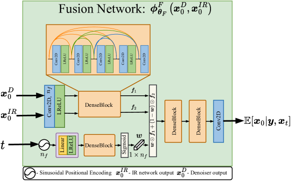
Figure 5: Detailed visualization of the proposed Fusion module.

Appendix I Fusion Module

The main goal of our proposed Fusion module is to predict the conditional expectation $\operatorname{\mathbb{E}}\left[\bm{x}_{0}|\bm{y},\bm{x}_{t}\right]$ given the estimates of $\operatorname{\mathbb{E}}\left[\bm{x}_{0}|\bm{x}_{t}\right]$ and $\operatorname{\mathbb{E}}\left[\bm{x}_{0}|\bm{y}\right]$, which are produced by the denoising and IR modules, respectively. To do so, our fusion network accepts as inputs the image estimates $\bm{x}_{0}^{D},\bm{x}_{0}^{IR}$ and a timestep $t$. Its exact architecture is depicted in Figure 5 and it consists of two branches. The upper branch operates on $\bm{x}_{0}^{D}$, $\bm{x}_{0}^{IR}$ and produces the corresponding features $\bm{f}_{1}$, $\bm{f}_{2}$ using a single dense block [27] without a normalization layer. The lower branch encodes the timestep $t$ into a vector of weights $\bm{w}\in\left(0,1\right)^{n_{f}}$ using the sinusoidal positional encoding [71], followed by a two layer MLP, and a sigmoid function as the final activation. Then, we perform a weighted summation of $\bm{f}_{1}$, $\bm{f}_{2}$ in the feature space. Finally, two consequent dense blocks [27], with $n_{f}$ channels each, followed by a convolution layer produce the final estimate of $\operatorname{\mathbb{E}}\left[\bm{x}_{0}|\bm{y},\bm{x}_{t}\right]$. Our proposed architecture has only 0.73M learnable parameters, which is significantly lower (7-22 times) compared to the Denoising and IR modules. As a result, the Fusion module requires less training time/resources and can be trained only on a small amount of problem-specific training data.

Table 11: Number of parameters and source code of methods used as an IR module in our framework.

IR Modules	Parameters $\downarrow$	Code & Weights
BSRT-Small	4.92M	link
FFTFormer	16.56M	link
SwinIR	11.85M	link

Appendix J Fusion Module Robustness

In order to assess the robustness/generalization ability of our method, we have conducted additional experiments where we evaluate the reconstruction quality achieved when the Fusion network, which was originally trained on the MIRNet-S and SwinIR pair, is combined with the following pairs of denosing and IR networks:

• The Fusion module is combined with the same pair of denoising and IR networks as those used during its training.

• The Fusion module is combined with a different IR network and the same denoising network as the one used during its training.

• The Fusion module is combined with a different denoising network and the same IR network as the one used during its training.

• The Fusion module is combined with different denoising and IR networks than the ones used during its training.

Table 12: The performance of Fusion module for different train/test pair scenarios for 4x SR task.

$\textnumero$	Trained Pair	Tested Pair	PSNR$\uparrow$	SSIM$\uparrow$	LPIPS$\downarrow$	TOPIQΔ$\downarrow$
-	Target		$\infty$	1	0	0
1	MIRNet-S + SwinIR	MIRNet-S + SwinIR	28.12	0.793	0.140	0.002
2	MIRNet-S + SwinIR	MIRNet-S + RRDB	28.20	0.795	0.144	0.023
3	MIRNet-S + SwinIR	UDP + SwinIR	28.47	0.808	0.177	0.017
4	MIRNet-S + SwinIR	UDP + RRDB	28.46	0.807	0.183	0.025

From these experiments as shown in the table above, we observe that changing the denoising network to a less powerful one leads to a noticeable drop in terms of perceptual quality ( 30% in LPIPS) and slightly blurrier results, which corresponds to a PSNR increase by 0.2dB. Conversely, altering the IR network has a minimal impact on both the reconstruction and perceptual metrics. In summary, under the particular IR task, the Fusion network evaluated with a different pair of denoising and IR modules demonstrates a good generalization ability and a robust behavior.

Appendix K Perception-Fidelity Trade-off

We have evaluated our method on the GoPro dataset (motion deblurring) for different $\tau$, when the denoising and Fusion modules are activated. From Table 13, we observe that the perception-fidelity trade-off follows a similar trend to the one for the SISR 4x task. The main difference is that in this particular case the necessary reverse diffusion steps are less than in SISR.

Table 13: Perception-Distortion Trade-off on GoPro validation for dynamic scene deblurring task.

$\tau$	0	1	5	10	20	25
PSNR, dB	34.21	34.02	33.72	33.52	33.23	33.14
LPIPS	0.071	0.057	0.053	0.052	0.052	0.052

Appendix L Information about Competing methods.

Below, we provide links to the code implementation and trained weights for all baselines used for comparison.

Table 14: Code and model weights of the competing methods for burst JDD-SR task.

Method	Link to Code	Link to Weights
DBSR	link	link
DeepRep	link	link
EBSR	link	link
BIPNet	link	link
BSRT	link	link

Table 15: Code and model weights of the competing methods for dynamic scene deblurring task.

Method	Link to Code	Link to Weights
HINet	link	link
MPRNet	link	link
MIMO-UNet+	link	link
NAFNet	link	link
Restormer	link	link
FFTFormer	link	link
DeblurGANv2	link	link

Table 16: Code and model weights of the competing methods for SISR task.

Method	Link to Code	Link to Weights
SRResNet	link	link
RRDB	link	link
SwinIR	link	link
LIIF	link	link
HAT	link	link
ESRGAN	link	link
HCFlow	link	link
SwinIR-GAN	link	link
LDM	link	link
SRDiff	link	link
IDM	link	link

Appendix M Additional Results

In the section, we provide additional visual comparison of the proposed method with existing SOTA approaches for all IR tasks under study.

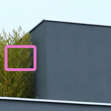
	DBSR: 0.144	DeepRep: 0.084	BSRT-Small: 0.048	BSRT-Large: 0.060
	Target	BIPNet: 0.069	EBSR: 0.054	Ours: 0.036

Figure 6: Visual comparison of our approach against competing methods on the Burst JDD-SR task (best viewed by zooming in). Every output image is accompanied by its LPIPS value.

	DBSR: 0.280	DeepRep: 0.270	BSRT-Small: 0.225	BSRT-Large: 0.258
	Target	BIPNet: 0.258	EBSR: 0.252	Ours: 0.131

Figure 7: Visual comparison of our approach against competing methods on the Burst JDD-SR task (best viewed by zooming in). Every output image is accompanied by its LPIPS value.

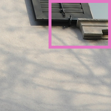
	DBSR: 0.160	DeepRep: 0.108	BSRT-Small: 0.081	BSRT-Large: 0.068
	Target	BIPNet: 0.089	EBSR: 0.083	Ours: 0.042

Figure 8: Visual comparison of our approach against competing methods on the Burst JDD-SR task (best viewed by zooming in). Every output image is accompanied by its LPIPS value.

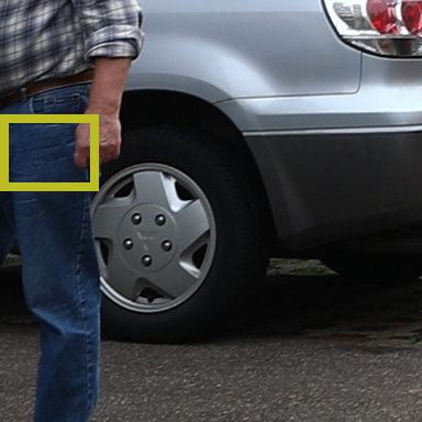
	DBSR: 0.165	DeepRep: 0.079	BSRT-Small: 0.036	BSRT-Large: 0.036
	Target	BIPNet: 0.043	EBSR: 0.035	Ours: 0.030

Figure 9: Visual comparison of our approach against competing methods on the Burst JDD-SR task (best viewed by zooming in). Every output image is accompanied by its LPIPS value.

	Input: 0.477	HINet: 0.128	Restormer: 0.135	DeblurGANv2: 0.195	InDI: 0.111
	Target	NAFNet: 0.112	FFTFormer: 0.094	DvSR: 0.106	Ours: 0.092

Figure 10: Visual comparison of our approach against competing methods on the GoPro test set for the task of dynamic scene deblurring (best viewed by zooming in). Every output image is accompanied by its LPIPS value.

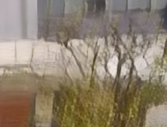
	Input: 0.547	HINet: 0.171	Restormer: 0.137	DeblurGANv2: 0.284	icDPM: 0.121
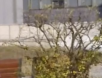
	Target	NAFNet: 0.133	FFTFormer: 0.122	DvSR: 0.127	Ours: 0.101

Figure 11: Visual comparison of our approach against competing methods on the GoPro test set for the task of dynamic scene deblurring (best viewed by zooming in). Every output image is accompanied by its LPIPS value.

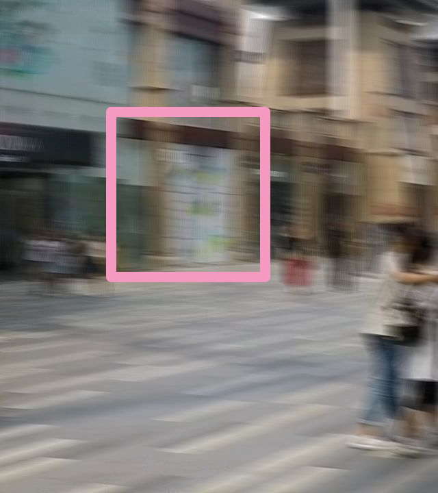
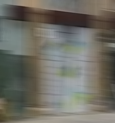
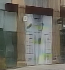
	Input: 0.533	HINet: 0.157	Restormer: 0.095	DeblurGANv2: 0.213	icDPM: 0.112
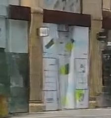
	Target	NAFNet: 0.086	FFTFormer: 0.105	DvSR: 0.134	Ours: 0.097

Figure 12: Visual comparison of our approach against competing methods on the HIDE test set for the task of dynamic scene deblurring (best viewed by zooming in). Every output image is accompanied by its LPIPS value.

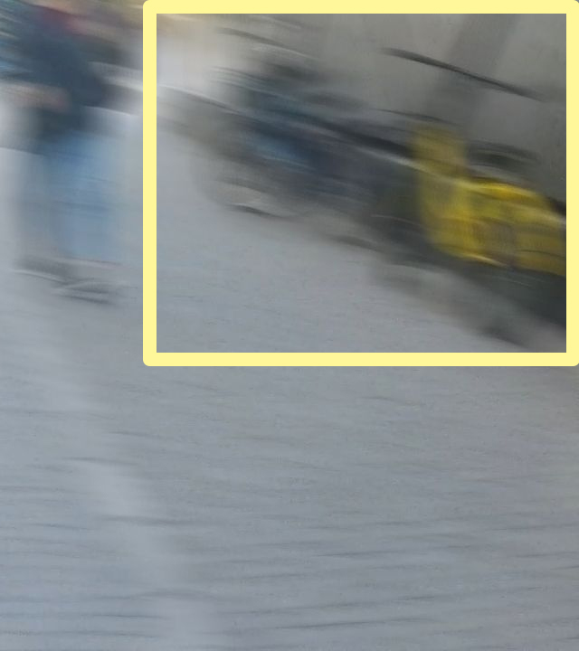
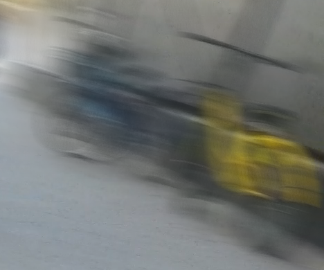
	Input: 0.402	HINet: 0.242	Restormer: 0.248	DeblurGANv2: 0.303	icDPM: 0.160
	Target	NAFNet: 0.207	FFTFormer: 0.182	DvSR: 0.192	Ours: 0.150

Figure 13: Visual comparison of our approach against competing methods on the HIDE test set for the task of dynamic scene deblurring (best viewed by zooming in). Every output image is accompanied by its LPIPS value.

	Input: 0.630	SwinIR: 0.056	HCFlow: 0.208	ESRGAN: 0.194	InDI: 0.245
	Target	HAT: 0.045	LDM: 0.273	SRDiff: 0.212	Ours: 0.048

Figure 14: Visual comparison of our approach against competing methods on the DIV2K validation set for the task of $4\times$ SISR (best viewed by zooming in). Every output image is accompanied by its LPIPS value.

	Input: 0.244	SwinIR: 0.102	HCFlow: 0.075	ESRGAN: 0.072	InDI: 0.074
	Target	HAT: 0.116	LDM: 0.190	SRDiff: 0.090	Ours: 0.072

Figure 15: Visual comparison of our approach against competing methods on the DIV2K validation set for the task of $4\times$ SISR (best viewed by zooming in). Every output image is accompanied by its LPIPS value.

	Input: 0.394	SwinIR: 0.114	HCFlow: 0.046	ESRGAN: 0.044	InDI: 0.057
	Target	HAT: 0.022	LDM: 0.141	SRDiff: 0.061	Ours: 0.022

Figure 16: Visual comparison of our approach against competing methods on the DIV2K validation set for the task of $4\times$ SISR (best viewed by zooming in). Every output image is accompanied by its LPIPS value.

	Input: 0.335	SwinIR: 0.230	HCFlow: 0.114	ESRGAN: 0.127	InDI: 0.194
	Target	HAT: 0.219	LDM: 0.269	SRDiff: 0.119	Ours: 0.140

Figure 17: Visual comparison of our approach against competing methods on the DIV2K validation set for the task of $4\times$ super-resolution (best viewed by zooming in). Every output image is accompanied by its LPIPS value.

References

- Agustsson and Timofte [2017] Eirikur Agustsson and Radu Timofte. Ntire 2017 challenge on single image super-resolution: Dataset and study. In The IEEE Conference on Computer Vision and Pattern Recognition (CVPR) Workshops, 2017.
- Arora et al. [2017] Sanjeev Arora, Rong Ge, Yingyu Liang, Tengyu Ma, and Yi Zhang. Generalization and equilibrium in generative adversarial nets (gans). In International conference on machine learning, pages 224–232. PMLR, 2017.
- Bascle et al. [1996] Benedicte Bascle, Andrew Blake, and Andrew Zisserman. Motion deblurring and super-resolution from an image sequence. In European conference on computer vision, pages 571–582. Springer, 1996.
- Bhat et al. [2021a] Goutam Bhat, Martin Danelljan, Luc Van Gool, and Radu Timofte. Deep burst super-resolution. In Proceedings of the IEEE/CVF Conference on Computer Vision and Pattern Recognition, pages 9209–9218, 2021a.
- Bhat et al. [2021b] Goutam Bhat, Martin Danelljan, Fisher Yu, Luc Van Gool, and Radu Timofte. Deep reparametrization of multi-frame super-resolution and denoising. In Proceedings of the IEEE/CVF International Conference on Computer Vision, pages 2460–2470, 2021b.
- Blau and Michaeli [2018] Yochai Blau and Tomer Michaeli. The perception-distortion tradeoff. In Proceedings of the IEEE Conference on Computer Vision and Pattern Recognition, pages 6228–6237, 2018.
- Brooks et al. [2019] Tim Brooks, Ben Mildenhall, Tianfan Xue, Jiawen Chen, Dillon Sharlet, and Jonathan T Barron. Unprocessing images for learned raw denoising. In Proceedings of the IEEE/CVF Conference on Computer Vision and Pattern Recognition, pages 11036–11045, 2019.
- Chen et al. [2023a] Chaofeng Chen, Jiadi Mo, Jingwen Hou, Haoning Wu, Liang Liao, Wenxiu Sun, Qiong Yan, and Weisi Lin. Topiq: A top-down approach from semantics to distortions for image quality assessment, 2023a.
- Chen et al. [2022] Honggang Chen, Xiaohai He, Linbo Qing, Yuanyuan Wu, Chao Ren, Ray E. Sheriff, and Ce Zhu. Real-world single image super-resolution: A brief review. Information Fusion, 79:124–145, 2022.
- Chen et al. [2023b] Xiangyu Chen, Xintao Wang, Jiantao Zhou, Yu Qiao, and Chao Dong. Activating more pixels in image super-resolution transformer. In Proceedings of the IEEE/CVF Conference on Computer Vision and Pattern Recognition, pages 22367–22377, 2023b.
- Chen et al. [2021] Yinbo Chen, Sifei Liu, and Xiaolong Wang. Learning continuous image representation with local implicit image function. In Proceedings of the IEEE/CVF conference on computer vision and pattern recognition, pages 8628–8638, 2021.
- Choi et al. [2022] Jooyoung Choi, Jungbeom Lee, Chaehun Shin, Sungwon Kim, Hyunwoo Kim, and Sungroh Yoon. Perception prioritized training of diffusion models. In Proceedings of the IEEE/CVF Conference on Computer Vision and Pattern Recognition, pages 11472–11481, 2022.
- Chung et al. [2022] Hyungjin Chung, Byeongsu Sim, and Jong Chul Ye. Come-closer-diffuse-faster: Accelerating conditional diffusion models for inverse problems through stochastic contraction. In Proceedings of the IEEE/CVF Conference on Computer Vision and Pattern Recognition, pages 12413–12422, 2022.
- Cohen et al. [2018] Joseph Paul Cohen, Margaux Luck, and Sina Honari. Distribution matching losses can hallucinate features in medical image translation. In International conference on medical image computing and computer-assisted intervention, pages 529–536. Springer, 2018.
- Delbracio and Milanfar [2023] Mauricio Delbracio and Peyman Milanfar. Inversion by direct iteration: An alternative to denoising diffusion for image restoration. Transactions on Machine Learning Research, 2023. Featured Certification.
- Dinh et al. [2014] Laurent Dinh, David Krueger, and Yoshua Bengio. Nice: Non-linear independent components estimation. arXiv preprint arXiv:1410.8516, 2014.
- Dudhane et al. [2022] Akshay Dudhane, Syed Waqas Zamir, Salman Khan, Fahad Shahbaz Khan, and Ming-Hsuan Yang. Burst image restoration and enhancement. In Proceedings of the IEEE/CVF Conference on Computer Vision and Pattern Recognition, pages 5759–5768, 2022.
- Elad and Feuer [1997] Michael Elad and Arie Feuer. Restoration of a single superresolution image from several blurred, noisy, and undersampled measured images. IEEE transactions on image processing, 6(12):1646–1658, 1997.
- Farsiu et al. [2004] Sina Farsiu, M Dirk Robinson, Michael Elad, and Peyman Milanfar. Fast and robust multiframe super resolution. IEEE transactions on image processing, 13(10):1327–1344, 2004.
- Gao et al. [2023] Sicheng Gao, Xuhui Liu, Bohan Zeng, Sheng Xu, Yanjing Li, Xiaoyan Luo, Jianzhuang Liu, Xiantong Zhen, and Baochang Zhang. Implicit diffusion models for continuous super-resolution. In Proceedings of the IEEE/CVF Conference on Computer Vision and Pattern Recognition, pages 10021–10030, 2023.
- Gatopoulos et al. [2020] Ioannis Gatopoulos, Maarten Stol, and Jakub M. Tomczak. Super-resolution variational auto-encoders, 2020.
- Goodfellow et al. [2014] Ian Goodfellow, Jean Pouget-Abadie, Mehdi Mirza, Bing Xu, David Warde-Farley, Sherjil Ozair, Aaron Courville, and Yoshua Bengio. Generative adversarial nets. Advances in neural information processing systems, 27, 2014.
- Guo et al. [2022] Baisong Guo, Xiaoyun Zhang, Haoning Wu, Yu Wang, Ya Zhang, and Yan-Feng Wang. Lar-sr: A local autoregressive model for image super-resolution. In Proceedings of the IEEE/CVF Conference on Computer Vision and Pattern Recognition, pages 1909–1918, 2022.
- Haar [1909] Alfred Haar. Zur theorie der orthogonalen funktionensysteme. Georg-August-Universitat, Gottingen., 1909.
- Hasinoff et al. [2016] Samuel W Hasinoff, Dillon Sharlet, Ryan Geiss, Andrew Adams, Jonathan T Barron, Florian Kainz, Jiawen Chen, and Marc Levoy. Burst photography for high dynamic range and low-light imaging on mobile cameras. ACM Transactions on Graphics (ToG), 35(6):1–12, 2016.
- Ho et al. [2020] Jonathan Ho, Ajay Jain, and Pieter Abbeel. Denoising diffusion probabilistic models. In Advances in Neural Information Processing Systems, pages 6840–6851. Curran Associates, Inc., 2020.
- Huang et al. [2017] Gao Huang, Zhuang Liu, Laurens Van Der Maaten, and Kilian Q Weinberger. Densely connected convolutional networks. In Proceedings of the IEEE conference on computer vision and pattern recognition, pages 4700–4708, 2017.
- Hyvärinen [2005] Aapo Hyvärinen. Estimation of non-normalized statistical models by score matching. Journal of Machine Learning Research, 6(24):695–709, 2005.
- Ignatov et al. [2020] Andrey Ignatov, Luc Van Gool, and Radu Timofte. Replacing mobile camera isp with a single deep learning model. In Proceedings of the IEEE/CVF Conference on Computer Vision and Pattern Recognition Workshops, pages 536–537, 2020.
- Johnson et al. [2016] Justin Johnson, Alexandre Alahi, and Li Fei-Fei. Perceptual losses for real-time style transfer and super-resolution. In Computer Vision–ECCV 2016: 14th European Conference, Amsterdam, The Netherlands, October 11-14, 2016, Proceedings, Part II 14, pages 694–711. Springer, 2016.
- Karras et al. [2022] Tero Karras, Miika Aittala, Timo Aila, and Samuli Laine. Elucidating the design space of diffusion-based generative models. In Proc. NeurIPS, 2022.
- Kingma and Ba [2014] Diederik P Kingma and Jimmy Ba. Adam: A method for stochastic optimization. arXiv preprint arXiv:1412.6980, 2014.
- Kingma and Welling [2014] Diederik P. Kingma and Max Welling. Auto-Encoding Variational Bayes. In 2nd International Conference on Learning Representations, ICLR 2014, 2014.
- Kong et al. [2023] Lingshun Kong, Jiangxin Dong, Jianjun Ge, Mingqiang Li, and Jinshan Pan. Efficient frequency domain-based transformers for high-quality image deblurring. In Proceedings of the IEEE/CVF Conference on Computer Vision and Pattern Recognition, pages 5886–5895, 2023.
- Kupyn et al. [2018] Orest Kupyn, Volodymyr Budzan, Mykola Mykhailych, Dmytro Mishkin, and Jiří Matas. Deblurgan: Blind motion deblurring using conditional adversarial networks. In Proceedings of the IEEE conference on computer vision and pattern recognition, pages 8183–8192, 2018.
- Kupyn et al. [2019] Orest Kupyn, Tetiana Martyniuk, Junru Wu, and Zhangyang Wang. Deblurgan-v2: Deblurring (orders-of-magnitude) faster and better. In The IEEE International Conference on Computer Vision (ICCV), 2019.
- Lecouat et al. [2021] Bruno Lecouat, Jean Ponce, and Julien Mairal. Lucas-kanade reloaded: End-to-end super-resolution from raw image bursts. In Proceedings of the IEEE/CVF International Conference on Computer Vision, pages 2370–2379, 2021.
- Ledig et al. [2017] Christian Ledig, Lucas Theis, Ferenc Huszár, Jose Caballero, Andrew Cunningham, Alejandro Acosta, Andrew Aitken, Alykhan Tejani, Johannes Totz, Zehan Wang, et al. Photo-realistic single image super-resolution using a generative adversarial network. In Proceedings of the IEEE conference on computer vision and pattern recognition, pages 4681–4690, 2017.
- Li et al. [2021] Haoying Li, Yifan Yang, Meng Chang, Huajun Feng, Zhihai Xu, Qi Li, and Yueting Chen. Srdiff: Single image super-resolution with diffusion probabilistic models. arXiv preprint arXiv:2104.14951, 2021.
- Li et al. [2023] Yawei Li, Yulun Zhang, Radu Timofte, Luc Van Gool, Lei Yu, Youwei Li, Xinpeng Li, Ting Jiang, Qi Wu, Mingyan Han, et al. Ntire 2023 challenge on efficient super-resolution: Methods and results. In Proceedings of the IEEE/CVF Conference on Computer Vision and Pattern Recognition, pages 1921–1959, 2023.
- Lian and Peng [2023] Wenyi Lian and Shanglian Peng. Kernel-aware burst blind super-resolution. In Proceedings of the IEEE/CVF Winter Conference on Applications of Computer Vision, pages 4892–4902, 2023.
- Liang et al. [2021a] Jingyun Liang, Jiezhang Cao, Guolei Sun, Kai Zhang, Luc Van Gool, and Radu Timofte. Swinir: Image restoration using swin transformer. In Proceedings of the IEEE/CVF international conference on computer vision, pages 1833–1844, 2021a.
- Liang et al. [2021b] Jingyun Liang, Andreas Lugmayr, Kai Zhang, Martin Danelljan, Luc Van Gool, and Radu Timofte. Hierarchical conditional flow: A unified framework for image super-resolution and image rescaling. In Proceedings of the IEEE/CVF International Conference on Computer Vision, pages 4076–4085, 2021b.
- Liao et al. [2021] Heng Liao, Jiajin Tu, Jing Xia, Hu Liu, Xiping Zhou, Honghui Yuan, and Yuxing Hu. Ascend: a scalable and unified architecture for ubiquitous deep neural network computing : Industry track paper. In 2021 IEEE International Symposium on High-Performance Computer Architecture (HPCA), pages 789–801, 2021.
- Lim et al. [2017] Bee Lim, Sanghyun Son, Heewon Kim, Seungjun Nah, and Kyoung Mu Lee. Enhanced deep residual networks for single image super-resolution. In Proceedings of the IEEE conference on computer vision and pattern recognition workshops, pages 136–144, 2017.
- Lugmayr et al. [2020] Andreas Lugmayr, Martin Danelljan, Luc Van Gool, and Radu Timofte. Srflow: Learning the super-resolution space with normalizing flow. In European Conference on Computer Vision, pages 715–732. Springer, 2020.
- Lugmayr et al. [2021] Andreas Lugmayr, Martin Danelljan, and Radu Timofte. Ntire 2021 learning the super-resolution space challenge. In Proceedings of the IEEE/CVF Conference on Computer Vision and Pattern Recognition, pages 596–612, 2021.
- Luo [2022] Calvin Luo. Understanding diffusion models: A unified perspective, 2022.
- Luo et al. [2021] Ziwei Luo, Lei Yu, Xuan Mo, Youwei Li, Lanpeng Jia, Haoqiang Fan, Jian Sun, and Shuaicheng Liu. Ebsr: Feature enhanced burst super-resolution with deformable alignment. In Proceedings of the IEEE/CVF Conference on Computer Vision and Pattern Recognition, pages 471–478, 2021.
- Luo et al. [2022] Ziwei Luo, Youwei Li, Shen Cheng, Lei Yu, Qi Wu, Zhihong Wen, Haoqiang Fan, Jian Sun, and Shuaicheng Liu. Bsrt: Improving burst super-resolution with swin transformer and flow-guided deformable alignment. In Proceedings of the IEEE/CVF Conference on Computer Vision and Pattern Recognition, pages 998–1008, 2022.
- Mehta et al. [2022] Nancy Mehta, Akshay Dudhane, Subrahmanyam Murala, Syed Waqas Zamir, Salman Khan, and Fahad Shahbaz Khan. Adaptive feature consolidation network for burst super-resolution. In Proceedings of the IEEE/CVF Conference on Computer Vision and Pattern Recognition, pages 1279–1286, 2022.
- Meng et al. [2022] Chenlin Meng, Yutong He, Yang Song, Jiaming Song, Jiajun Wu, Jun-Yan Zhu, and Stefano Ermon. SDEdit: Guided image synthesis and editing with stochastic differential equations. In International Conference on Learning Representations, 2022.
- Nah et al. [2017] Seungjun Nah, Tae Hyun Kim, and Kyoung Mu Lee. Deep multi-scale convolutional neural network for dynamic scene deblurring. In The IEEE Conference on Computer Vision and Pattern Recognition (CVPR), 2017.
- Nguyen et al. [2017] A. Nguyen, J. Clune, Y. Bengio, A. Dosovitskiy, and J. Yosinski. Plug & play generative networks: Conditional iterative generation of images in latent space. In 2017 IEEE Conference on Computer Vision and Pattern Recognition (CVPR), pages 3510–3520, Los Alamitos, CA, USA, 2017. IEEE Computer Society.
- Nichol and Dhariwal [2021a] Alex Nichol and Prafulla Dhariwal. Improved denoising diffusion probabilistic models. arXiv preprint arXiv:2102.09672, 2021a.
- Nichol and Dhariwal [2021b] Alexander Quinn Nichol and Prafulla Dhariwal. Improved denoising diffusion probabilistic models. In Proceedings of the 38th International Conference on Machine Learning, pages 8162–8171. PMLR, 2021b.
- Prakash et al. [2020] Mangal Prakash, Alexander Krull, and Florian Jug. Fully unsupervised diversity denoising with convolutional variational autoencoders. In International Conference on Learning Representations, 2020.
- Ren et al. [2020] Dongwei Ren, Kai Zhang, Qilong Wang, Qinghua Hu, and Wangmeng Zuo. Neural blind deconvolution using deep priors. In Proceedings of the IEEE/CVF Conference on Computer Vision and Pattern Recognition, pages 3341–3350, 2020.
- Ren et al. [2023] Mengwei Ren, Mauricio Delbracio, Hossein Talebi, Guido Gerig, and Peyman Milanfar. Multiscale structure guided diffusion for image deblurring. In Proceedings of the IEEE/CVF International Conference on Computer Vision, pages 10721–10733, 2023.
- Rombach et al. [2022] Robin Rombach, Andreas Blattmann, Dominik Lorenz, Patrick Esser, and Björn Ommer. High-resolution image synthesis with latent diffusion models. In Proceedings of the IEEE/CVF Conference on Computer Vision and Pattern Recognition (CVPR), pages 10684–10695, 2022.
- Saharia et al. [2021] Chitwan Saharia, Jonathan Ho, William Chan, Tim Salimans, David J Fleet, and Mohammad Norouzi. Image super-resolution via iterative refinement. arXiv preprint arXiv:2104.07636, 2021.
- Salimans et al. [2016] Tim Salimans, Ian Goodfellow, Wojciech Zaremba, Vicki Cheung, Alec Radford, and Xi Chen. Improved techniques for training gans. Advances in neural information processing systems, 29, 2016.
- Schultz and Stevenson [1996] Richard R Schultz and Robert L Stevenson. Extraction of high-resolution frames from video sequences. IEEE transactions on image processing, 5(6):996–1011, 1996.
- Shen et al. [2019] Ziyi Shen, Wenguan Wang, Jianbing Shen, Haibin Ling, Tingfa Xu, and Ling Shao. Human-aware motion deblurring. In IEEE International Conference on Computer Vision, 2019.
- Sohl-Dickstein et al. [2015] Jascha Sohl-Dickstein, Eric Weiss, Niru Maheswaranathan, and Surya Ganguli. Deep unsupervised learning using nonequilibrium thermodynamics. In Proceedings of the 32nd International Conference on Machine Learning, pages 2256–2265. PMLR, 2015.
- Song et al. [2021a] Jiaming Song, Chenlin Meng, and Stefano Ermon. Denoising diffusion implicit models. In International Conference on Learning Representations, 2021a.
- Song et al. [2021b] Yang Song, Jascha Sohl-Dickstein, Diederik P Kingma, Abhishek Kumar, Stefano Ermon, and Ben Poole. Score-based generative modeling through stochastic differential equations. In International Conference on Learning Representations, 2021b.
- Sun et al. [2018] Deqing Sun, Xiaodong Yang, Ming-Yu Liu, and Jan Kautz. Pwc-net: Cnns for optical flow using pyramid, warping, and cost volume. In Proceedings of the IEEE conference on computer vision and pattern recognition, pages 8934–8943, 2018.
- Tsai et al. [2022] Fu-Jen Tsai, Yan-Tsung Peng, Yen-Yu Lin, Chung-Chi Tsai, and Chia-Wen Lin. Stripformer: Strip transformer for fast image deblurring. In European Conference on Computer Vision, pages 146–162. Springer, 2022.
- Tsai [1984] R Tsai. Multiframe image restoration and registration. Advance Computer Visual and Image Processing, 1:317–339, 1984.
- Vaswani et al. [2017] Ashish Vaswani, Noam Shazeer, Niki Parmar, Jakob Uszkoreit, Llion Jones, Aidan N Gomez, Łukasz Kaiser, and Illia Polosukhin. Attention is all you need. Advances in neural information processing systems, 30, 2017.
- Vincent [2011] Pascal Vincent. A connection between score matching and denoising autoencoders. Neural Computation, 23(7):1661–1674, 2011.
- Wang et al. [2018] Xintao Wang, Ke Yu, Shixiang Wu, Jinjin Gu, Yihao Liu, Chao Dong, Yu Qiao, and Chen Change Loy. Esrgan: Enhanced super-resolution generative adversarial networks. In Proceedings of the European conference on computer vision (ECCV) workshops, pages 0–0, 2018.
- Wang et al. [2019] Xintao Wang, Kelvin CK Chan, Ke Yu, Chao Dong, and Chen Change Loy. Edvr: Video restoration with enhanced deformable convolutional networks. In Proceedings of the IEEE/CVF Conference on Computer Vision and Pattern Recognition Workshops, pages 0–0, 2019.
- Wang et al. [2021] Xintao Wang, Liangbin Xie, Chao Dong, and Ying Shan. Real-esrgan: Training real-world blind super-resolution with pure synthetic data. In Proceedings of the IEEE/CVF international conference on computer vision, pages 1905–1914, 2021.
- Wang et al. [2023] Yinhuai Wang, Jiwen Yu, and Jian Zhang. Zero-shot image restoration using denoising diffusion null-space model. In The Eleventh International Conference on Learning Representations, 2023.
- Wang et al. [2004] Zhou Wang, Alan C Bovik, Hamid R Sheikh, and Eero P Simoncelli. Image quality assessment: from error visibility to structural similarity. IEEE transactions on image processing, 13(4):600–612, 2004.
- Whang et al. [2022] Jay Whang, Mauricio Delbracio, Hossein Talebi, Chitwan Saharia, Alexandros G Dimakis, and Peyman Milanfar. Deblurring via stochastic refinement. In Proceedings of the IEEE/CVF Conference on Computer Vision and Pattern Recognition, pages 16293–16303, 2022.
- Wronski et al. [2019] Bartlomiej Wronski, Ignacio Garcia-Dorado, Manfred Ernst, Damien Kelly, Michael Krainin, Chia-Kai Liang, Marc Levoy, and Peyman Milanfar. Handheld multi-frame super-resolution. ACM Transactions on Graphics (TOG), 38(4):1–18, 2019.
- Xia et al. [2023] Bin Xia, Yulun Zhang, Shiyin Wang, Yitong Wang, Xinglong Wu, Yapeng Tian, Wenming Yang, and Luc Van Gool. Diffir: Efficient diffusion model for image restoration. In Proceedings of the IEEE/CVF International Conference on Computer Vision (ICCV), pages 13095–13105, 2023.
- Zamir et al. [2020] Syed Waqas Zamir, Aditya Arora, Salman Khan, Munawar Hayat, Fahad Shahbaz Khan, Ming-Hsuan Yang, and Ling Shao. Learning enriched features for real image restoration and enhancement. In Computer Vision–ECCV 2020: 16th European Conference, Glasgow, UK, August 23–28, 2020, Proceedings, Part XXV 16, pages 492–511. Springer, 2020.
- Zamir et al. [2021] Syed Waqas Zamir, Aditya Arora, Salman Khan, Munawar Hayat, Fahad Shahbaz Khan, Ming-Hsuan Yang, and Ling Shao. Multi-stage progressive image restoration. In Proceedings of the IEEE/CVF Conference on Computer Vision and Pattern Recognition (CVPR), pages 14821–14831, 2021.
- Zamir et al. [2022] Syed Waqas Zamir, Aditya Arora, Salman Khan, Munawar Hayat, Fahad Shahbaz Khan, and Ming-Hsuan Yang. Restormer: Efficient transformer for high-resolution image restoration. In Proceedings of the IEEE/CVF conference on computer vision and pattern recognition, pages 5728–5739, 2022.
- Zhai et al. [2023] Lujun Zhai, Yonghui Wang, Suxia Cui, and Yu Zhou. A comprehensive review of deep learning-based real-world image restoration. IEEE Access, 11:21049–21067, 2023.
- Zhang et al. [2020] Kaihao Zhang, Wenhan Luo, Yiran Zhong, Lin Ma, Bjorn Stenger, Wei Liu, and Hongdong Li. Deblurring by realistic blurring. In Proceedings of the IEEE/CVF Conference on Computer Vision and Pattern Recognition, pages 2737–2746, 2020.
- Zhang et al. [2018] Richard Zhang, Phillip Isola, Alexei A. Efros, Eli Shechtman, and Oliver Wang. The unreasonable effectiveness of deep features as a perceptual metric. In Proceedings of the IEEE Conference on Computer Vision and Pattern Recognition (CVPR), 2018.
- Zhang et al. [2021] Wenlong Zhang, Yihao Liu, Chao Dong, and Yu Qiao. Ranksrgan: Super resolution generative adversarial networks with learning to rank. IEEE Transactions on Pattern Analysis and Machine Intelligence, 44(10):7149–7166, 2021.
- Zhao et al. [2016] Hang Zhao, Orazio Gallo, Iuri Frosio, and Jan Kautz. Loss functions for image restoration with neural networks. IEEE Transactions on computational imaging, 3(1):47–57, 2016.
- Zou et al. [2023] Zhengxia Zou, Keyan Chen, Zhenwei Shi, Yuhong Guo, and Jieping Ye. Object detection in 20 years: A survey. Proceedings of the IEEE, 111(3):257–276, 2023.