Ansatz about a zero momentum mode in QCD and the forward slope in pp elastic scattering

Abstract

We recall a resummation procedure in QED to extract the zero momentum mode in soft photon emission and present an ansatz about a possible mechanism for the forward peak characterizing elastic proton proton scattering.

I Introduction

The observation of the rise of the total proton-proton cross-section at the Intersecting Storage Rings (ISR) accelerator Amaldi et al. (1973) was one of the earliest signals of non scaling phenomena in hadronic physics, as surprises arrived when the increasing proton c.m. energy passed the threshold between quark confinement and asymptotic freedom. The rise had been anticipated by cosmic ray observations Yodh et al. (1972), and was among other unexpected results, such as the excess in multi hadron production in electron-positron collisions, first observed at ADONE, when it started its operation in 1969 with $\sqrt{s}\approx 1.6-2$ GeV Bartoli et al. (1970). The observation was soon confirmed at the Cambridge Electron Accelerator and later at SPEAR, showing that a threshold had been passed as it became quantitatively evident a few years later, in November 1974, with the discovery of a new particle, later called the $J/\Psi$-meson. It was a bound state of a new quark, the charm, a very narrow resonance with $3.1$ GeV mass Aubert et al. (1974); Augustin et al. (1974); Bacci et al. (1974), an energy at which the strong coupling constant can be expected to be small enough to allow a perturbative behaviour De Rujula and Glashow (1975).

Similarly, in hadron interactions, the observation of the rise of the total $p-p$ cross-section can be expected when the c.m. energy for parton-parton collisions is around 2-3 GeV, which would correspond to $E_{cm}^{pp}\approx 20$ GeV, in a simple model where each quark in the proton carries 1/6 of the energy Fagundes et al. (2015). Indeed, a rising behaviour, which one can attribute to semi-hard collisions, had been reported to appear in cosmic rays experiments in 1972 Yodh et al. (1972) and was confirmed when the ISR Amaldi et al. (1971, 1973) started taking data for the total and elastic cross-sections. Further experimental studies of the elastic differential cross-section gave evidence for structure in $pp$ collisions. As to the detailed mechanism for the rise of $\sigma_{total}$, we have long advocated for the rise being a collective effect of mini-jet production, accompanied by soft gluon resummation. Namely, the rise is due to the appearance of interacting quarks and gluons and it is modulated by the unavoidable soft gluon emission.The problem of such model to be quantitative is the still not understood behaviour of the strong interaction coupling for very small momentum, near zero, soft gluons.

In previous publications Godbole et al. (2005), we have been able to describe the energy dependence of the total $pp/{\bar{p}}$ cross-section Pancheri and Srivastava (2017) through currently available LO PDF for parton parton collisions, and an infrared safe resummation procedure with a singular but integrable coupling constant $\alpha_{s}(k_{t})$ such that

$$\alpha_{s}^{IR}(k_{t})=\frac{12\pi}{11N_{c}-2N_{f}}(\frac{k_{t}^{2}}{\Lambda^{2}})^{-p}\ \ \ \ \ p<1$$ (1)

$$\alpha_{s}^{AF}(k_{t})=\frac{12\pi}{11N_{c}-2N_{f}}\log[\frac{k_{t}^{2}}{\Lambda^{2}}]$$ (2)

where Eq. (1) ensures infrared integrability for the resummation procedure, and Eq. (2) appropriately describes perturbative behaviour for the mini-jet collisions. In our published phenomenology Godbole et al. (2005); Achilli et al. (2011) we used an interpolating expression

$$\alpha_{s}^{BN}(k_{t})=\frac{12\pi}{11N_{c}-2N_{f}}\frac{p}{\log[1+p(\frac{k_{t}}{\Lambda})^{2p}]}$$ (3)

We called BN model our proposal for the rising total pp cross-section, from the Bloch and Nordsieck Bloch and Nordsieck (1937) theorem, which inspired Touschek’s soft photon resummation procedure Etim et al. (1967), which we have extended to treat soft gluon emission during the semi-hard collision. Such a model was based on eikonal resummation of QCD mini-jets Durand and Pi (1988), with an impact parameter distribution inspired by our previous work on soft gluon effects in hadronic collisions Pancheri-Srivastava and Srivastava (1977). The BN model reproduced total cross-section data up to LHC energies and available cosmic ray data within reported errors, but unlike other models Jenkovszky (2023); Khoze et al. (2018); Luna et al. (2024) could not reproduce the elastic or quasi-elastic process, and underestimated the total inelastic cross-section, as shown in Figs (1) Pancheri et al. (2014). This difficulty could be due to our model, based so far on a single channel component. Presently, we refrain from going beyond the one channel Ryskin et al. (2009), as this would introduces extra parameters.

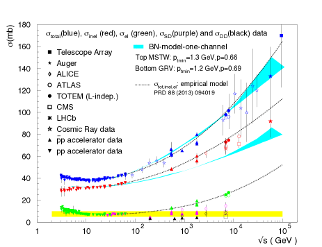
Figure 1: The figure Pancheri et al. (2014) shows the total, elastic and inelastic cross-section in the BN model (blue band)Godbole et al. (2005), and an empirical model (dots) Fagundes et al. (2013). The yellow band is the diffractive contribution from data.

As for the differential cross-section, the BN model did not show a dip structure (only bumps and zeroes) Jenkovszky et al. (2024) nor an exponential behaviour for $-q^{2}\approx 0$, as observed in the forward peak Fagundes et al. (2016). Such behaviour can be obtained in Regge-type models but did not naturally arise in our BN model.

To test the forward region, an empirical $bmax$ can be introduced to multiply the differential cross-section from our model at $\sqrt{s}=13$ TeV, obtaining a good description of data Antchev et al. (2019) up to the bump, as shown in Fig. 2.

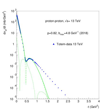
Figure 2: TOTEM 13 TeV data and the BN model with an exponential cut-off, plot courtesy from A. Grau.

In order to understand the origin of a cut-off in QCD in the context of our model, we now turn to address the question of zero momentum modes in gauge theories Palumbo (1983). After summarizing both the Touschek resummation method in QED and its extension to deal with zero momentum modes, we will propose an ansatz for the origin of the forward peak, based on a revisitation of the Touschek’s procedure. The ansatz we present has a correspondance with Color Condensate Models, but differs in that we derive its origin from the zero mode in soft emission processes resummed through the Touschek method Etim et al. (1967); Palumbo and Pancheri (1984).

In Sect. II we recollect the results from previous work about the zero momentum mode in Abelian gauge theories. We then extend the discussion to the transverse momentum distribution in QCD and show how hadronic processes could exhibit a forward peak in the elastic differential cross-section, arising from the zero momentum mode. We shall then have a discussion about the proposed expression for the interpolating $\alpha_{s}$, Sect. IV, leaving the relevant phenomenology to a further publication. The article will close with some considerations about the strong coupling constant in its two asymptotic limits.

II Zero momentum mode in Abelian gauge theories

Our argument would follow two papers Palumbo and Pancheri (1984); Palumbo (1983) about the connection between boundary conditions in gauge theories and its implications following the possible existence of zero momentum modes. The question had been posed whether unexpected physical effects can rise in the transition from a sum over discrete modes to continuum distributions Palumbo (1983). Using the Fourier expansion of the gauge fields, it was argued that the gauge field should vanish at the boundaries of the QED quantization box, whereas the question arises whether periodic boundary conditions in QCD might give observable effects. The problem was rediscussed Palumbo and Pancheri (1984), using Bruno Touschek resummation formalism Etim et al. (1967), EPT for short, based on a semi-classical approach to calculate the probability distribution of soft photons, emitted in charged particles collisions.

II.1 Touschek’s formalism for QED

Touschek’s objective was to calculate the probability of unobserved soft photon emission up to an experimental resolution $\Delta\omega\leq E$, the scale of the process and obtain the correction factor to the measured electron-positron cross-section. Touschek started with the Bloch and Nordsieck result about soft photon emission from a classical source Bloch and Nordsieck (1937). Bloch and Nordsieck had shown that the distribution in the number of photons was given by a Poisson distribution, hence the probability of emission of soft photons with different values for the momentum k would be given by the product of their Poisson distributions, namely

$$P(\{n_{\bf k}\})=\Pi_{\bf k}\frac{{\bar{n}}_{\bf k}^{n_{\bf k}}}{n_{\bf k}!}\rm{exp}[-{\bar{n}}_{\bf k}]$$ (4)

with $n_{\bf k}$ the number of photons emitted with momentum ${\bf k}$ around their average value ${\bar{n}}_{\bf k}$. We notice that Eq. (4) describes a discrete momentum spectrum of the emitted photons, corresponding to quantization of the electromagnetic field in a finite box. In the following, we shall first assume that a smooth continuum limit exists. As we go through Touschek’s argument, we shall also point out possible subtleties with the continuum limit.

The next four steps taken by Touschek are:

1. sum over all values of number of soft photons of momentum k, namely

   $$\sum_{n_{\bf k}}P(\{n_{\bf k}\})$$ (5)

2. the probability of having a 4 -momentum loss between $K_{\mu}$ and $K_{\mu}+d^{4}K$ due to all possible number of emitted photons $n_{\bf k}$ and all possible single photon momentum k, is obtained by imposing overall energy momentum conservation, through the function $\delta^{4}(K_{\mu}-\sum_{\bf k}n_{\bf k}k_{\mu})$ expressed in its $\mathcal{F}ourier$ trasform

   $$\delta^{4}(K_{\mu}-\sum_{\bf k}n_{\bf k}k_{\mu})=\frac{1}{(2\pi)^{4}}\int d^{4}xe^{-i(K_{\mu}-\sum_{\bf k}n_{\bf k}k_{\mu})\cdot x}$$ (6)

3. one can then exchange the product of the infinite number of Poisson distributions, Eq. (4) with the sum in Eq. (5),

4. and take the continuum limit, unless there are special boundary conditions, as discussed in the next section.

In the following we shall refer to this work as EPT paper. Explicitly, the above steps are implemented as

$$d^{4}P(K)=\sum_{n_{\bf k}}P(\{n_{\bf k}\})d^{4}{K}\delta_{4}(K-\sum_{\bf k}kn_{\bf k})=$$

$$\sum_{n_{k}}\Pi_{\bf k}\frac{[\bar{n}_{\bf k}]^{n_{\bf k}}}{n_{\bf k}!}e^{-\bar{n}_{\bf k}}d^{4}{K}\delta_{4}({K}-\sum_{\bf k}{k}n_{\bf k})$$ (7)

Touschek proceeds to steps 2 & 3 by using the integral representation of the delta-function to exchange the sum with the product obtaining

$$d^{4}P(K)=\frac{d^{4}K}{(2\pi)^{4}}\int d^{4}xe^{-i{K\cdot x}}exp\{-\sum_{\bf k}{\bar{n}}_{\bf k}[1-e^{ik\cdot x}]\}$$ (8)

Going to the continuum, brings

$$d^{4}P(K)=\frac{d^{4}K}{(2\pi)^{4}}\int d^{4}xe^{-iK\cdot x}exp\{-\int d^{3}{\bar{n}}_{\bf k}[1-e^{ik\cdot x}]\}$$ (9)

In this formulation, an important property of the integrand in Eqs. (8) and (9) is that by its definition $d^{4}P(K)\neq 0$ only for $K_{0}\equiv\omega\geq 0$, since for each single photon $k_{0}\geq 0$ .

II.2 The continuum limit and the closed form expression for the energy distribution

If one takes the continuum limit, integrating over the three momentum $\bf K$ leads to the probability of finding an energy loss in the interval $d\omega$ as

$$dP(\omega)=\frac{d\omega}{2\pi}\int_{-\infty}^{+\infty}dt\ \rm{exp[i\omega\ t-h(t)]}=$$

$$\frac{d\omega}{2\pi}\int_{-\infty}^{+\infty}dt\ \rm{exp[i\omega\ t-\beta(\alpha_{em};p_{i}^{\mu})\int_{o}^{\epsilon_{s}}\frac{dk}{k}(1-e^{-ikt})]}$$ (10)

where one has used the property of separation between the angular and the momentum integration over the photon momenta, already exploited by Weinberg Weinberg (1965), and known to previous authors as well. The separation defines $\beta(\alpha_{em};p_{i}^{\mu})=\beta$ as a function of the incoming and outgoing particle momenta $(p_{i}^{\mu})$, i.e.

$$\beta=\frac{\alpha}{(2\pi)^{2}}\int d^{2}{\bf n}\sum_{\hat{e}}|\sum_{i}\frac{(p_{i}\cdot{\hat{e}})\epsilon_{i}}{({\bf p}_{i}\cdot{\hat{n}}-p_{0i})}|^{2}$$ (11)

where $p_{i}$ and ${\hat{e}}$ are the 4-momenta and polarization of the incoming and outgoing particles, $\epsilon_{i}=\pm 1$, for incoming particles or antiparticles; $\epsilon_{s}$ an energy scale valid for single soft photon emission, to be determined to the order of precision in the perturbation treatment of the process to be studied. The function $\beta$ was shown to be a relativistic invariant Etim et al. (1967) and its expression in terms of the Mandelstam variables $s,t,u$ of two charged particle scattering can be written as Pancheri-Srivastava (1973):

$$\beta=\beta(s,t,u)=\frac{2e^{2}}{\pi}[-I_{12}+I_{13}+I_{14}-2]$$ (12)

where

$$I_{ij}=2(p_{i}\cdot p_{j})\int_{0}^{1}\frac{dy}{2y(1-y)[(p_{i}\cdot p_{j})-m_{e}^{2}]+m_{e}^{2}}$$ (13)

with the high energy limit $s$, $u\rightarrow\infty$, $-t\rightarrow 0$, $\beta\rightarrow-t/m_{e}$, which follows from the existence of the constant term in Eq. (12).

Following the steps taken from Eq. [11] through Eq.  [17] of the EPT paper Etim et al. (1967), the analyticity properties of $h(t)$ in the lower half of the $t$-plane resulting from the constraint that $\omega\geq 0$, lead to

$$N(\beta)dP(\omega)=\beta\frac{d\omega}{\omega}(\frac{\omega}{E})^{\beta}\ \ \ \ \ for\ \omega<E$$ (14)

with the normalization factor given by

$$N(\beta)=\frac{\int_{0}^{\infty}dP(\omega)}{\int_{0}^{E}dP(\omega)}=\gamma^{\beta}\Gamma(1+\beta)$$ (15)

which one obtains following the procedure outlined in Appendix III of the paper.

II.3 The zero momentum mode

In this section we return to Eq. (8) and discuss the separation of the zero momentum mode from the continuum, in Abelian gauge theories for different boundary conditions Palumbo and Pancheri (1984).

Up to Eq. (8), the method developed to obtain the energy-momentum distribution $K_{\mu}$ is a classical statistical mechanics exercise. Going further requires an expression for the average number of photons of momentum $\bf k$ and the choice of the boundary conditions imposed upon the field. Before taking the continuum limit, it has been suggested Palumbo and Pancheri (1984) to separate the zero mode from the others. Let the quantization volume be $V=L^{3}$, and introduce $\mu$, a fictitious photon mass, in light of eventually take the limit $L\rightarrow\infty$ and $\mu\rightarrow 0$. Separating the zero momentum mode of energy $\omega_{0}$ from all the other modes, we write

$$h(t)=n_{0}[1-e^{-i\omega_{0}t}]+{\bar{h}}(t)=n_{0}[1-e^{-i\omega_{0}t}]+$$

$$+\beta\int_{o}^{E}\frac{dk}{k}[1-e^{-ikt}];$$

with the photon mass now safely taken to be zero in the integral defining ${\bar{h}}(t)$. For the zero mode, the $\mu\rightarrow 0$ limit require more attention. One has

$$n_{0}[1-e^{-i\omega_{0}t}]\approx in_{0}\omega_{0}t\rightarrow in_{0}\mu t\equiv iW_{0}t$$ (17)

We see that the zero momentum mode can introduce a new energy scale $W_{0}$, namely

$$W_{0}=\frac{4\pi e^{2}\mu}{L^{3}\mu^{3}}\times\frac{1}{2}|\sum_{i}\epsilon_{i}\vec{v}_{i}|^{2}\equiv G(\mu)F(E,m)$$ (18)

with the finite dimensionless function $F(E,m)=|\sum_{i}\epsilon_{i}{\bf v_{i}}|^{2}/2$ depending on mass and energy of the emitting particles.

The overall energy distribution can now be written

$$dP(\omega)=\frac{d\omega}{2\pi}\int\ dt\ e^{i(\omega-W_{0})t-{\bar{h}}(t)}$$ (19)

The question is how to take the continuum limit, $L\rightarrow\infty$ and $\mu\rightarrow 0$ and, accordingly whether the energy $W_{0}$ can be finite. Various cases can be considered, in correspondence with different boundary conditions, as will be discussed in a separate publication. Here we only note that if the limit to be taken is $\lim_{L\rightarrow\infty,\mu\rightarrow 0}L^{3}\mu^{3}=finite$, then $W_{0}=0$ in QED but $W_{0}\neq 0$ can happen if $e^{2}\mu\rightarrow finite$ in this limit. In such case the energy distribution would receive an extra contribution to the usual QED expression. Following the same derivation as in Etim et al. (1967) - based on the analyticity properties of the energy distribution for extracting $dP(\omega)$ for $\omega\leq E$, one obtains

$$(\frac{\omega}{E})^{\beta}\rightarrow(\frac{\omega}{E})^{\beta}\ (1-\frac{W_{0}}{\omega})^{\beta}$$ (20)

It should be noticed that the extra factor $(1-\frac{W_{0}}{\omega})^{\beta}$ is regulated by the continuum contribution through the $\beta$ exponent.

III How about QCD?

The interest in the separation between the zero momentum from the continuum arises in QCD, in particular for the case of the transverse momentum distribution of the emitted radiation. Integrating the four momentum distribution over the energy and the longitudinal momentum variable, one can write the overall $d^{2}P({\bf K}_{\perp})$ distribution Pancheri-Srivastava and Srivastava (1977) as follows:

$$d^{2}P({\bf K}_{\perp})=\frac{1}{(2\pi)^{2}}\int d^{2}{\bf b}e^{-i{\bf K}_{\perp}\cdot{\bf b}-\sum_{\bf k}\bar{n}_{\bf k}[1-e^{i{\bf k}_{t}\cdot{\bf b}}]}$$ (21)

where $\bar{n}_{\bf k}$ is the average number of soft gluons emitted with momentum ${\bf k}$. Taking a straightforward continuum limit, this expression leads to the expression for soft gluon transverse momentum distribution

$$d^{2}P({\bf K}_{\perp})=\frac{1}{(2\pi)^{2}}\int d^{2}{\bf b}e^{-i{\bf K}_{\perp}\cdot{\bf b}-h({\bf b})}$$ (22)

with

$$h(b)=\int^{qmax}d^{2}{\bf k}_{t}\frac{\alpha_{s}(k_{t})}{k_{t}^{2}}\ln({2qmax/k_{t}})[1-e^{i{\bf k}_{t}\cdot{\bf b}}]$$ (23)

with $qmax$ an upper limit of integration which depends on the process under consideration. The still unknown infrared behaviour of $\alpha_{s}$ led the lower limit of integration to be a scale $\Lambda\neq 0$ Dokshitzer et al. (1978); Parisi and Petronzio (1979); Curci et al. (1979), introducing an intrinsic transverse momentum for phenomenological applicationsHayrapetyan et al. (2024). In our phenomenology of hadronic cross-sections, we have set the lower limit to be zero, introducing a singular but integrable behaviour for $\alpha_{s}$ in the infrared region as highlighted in the Introduction, through Eq. (3). As a result, the integration is now dominated by a power law behaviour of $\alpha_{s}$ for $k_{t}\lesssim\Lambda$, and morphs into the asymptotic freedom expression beyond it. More about this issue will be discussed in Sect. IV.

However, just as in the case of the energy distribution that we have previously discussed, care is needed in taking the continuum limit, and one must first separate out the zero momentum mode, with the result that the distribution now takes the form

$$d^{2}P({\bf K}_{\perp})=\frac{1}{(2\pi)^{2}}\int d^{2}{\bf b}e^{-i{\bf K}_{\perp}\cdot{\bf b}-\nu^{2}b^{2}-h_{continuum}({b})}$$ (24)

with

$$h_{continuum}(b)=\int_{0}^{qmax}d^{3}\bar{n}_{\bf k}[1-e^{i{\bf k}_{t}\cdot{\bf b}}]$$ (25)

given in Eq. 23. In Eq. 24 we argue that a cut off in impact space is developed through the zero momentum mode ${\bf n}_{0}[1-e^{i{\bf k}_{t}\cdot{\bf b}}]\approx{\bf n}_{0}[-i{\bf k}_{t}\cdot{\bf b}]+{\bf n}_{0}\mu^{2}b^{2}+...\approx\nu^{2}b^{2}$, as the first term in the square bracket is killed by the integration over all directions, and only the second term remains. The coefficient $\nu^{2}=\mu^{2}{\bf n}_{0}$ would be calculated by taking the zero mode limit of $\bar{n}_{\bf k}$ and is the analogue of the parameter $W_{0}$ discussed in the previous section for the energy distribution in an Abelian theory.

We see that the Touschek resummation procedure, that began with statistical mechanics manipulations, can be applied to go beyond the derivation of the well known exponentiation of infrared corrections. In this section, we have used it to explore the possibility of the appearance of a cut-off in impact parameter space arising from the zero momentum mode in QCD. Whether such a term survives and manifests itself as the origin of the forward slope of the elastic differential $p-p/{\bar{p}}$ cross-ssection would depend upon whether the cut-off $\nu\neq 0$ in the zero momentum limit.

Thus the question is not only to perform the integral for the continuum in Eq. (25) in the unknown infrared region, but also to examine possible limits of the cut-off scale $\nu$ in a theory such as QCD, inspecting the zero momentum mode. These could be two different regimes, and need not require the same treatment.

In previous publications we have in fact proposed to evaluate $\bar{n}_{\bf k}$ using a singular but integral expression for the strong coupling constant and we shall discuss it in Sect. IV, which we now turn to.

IV Modelling the strong coupling constant in soft gluon resummation

IV.1 Models for $\alpha_{s}$ in the continuum

The ansatz in Eq. (3), on which we relied for our previous phenomenology for the hadronic cross-section, is however unsatisfactory, as it introduced a parameter $1/2<p<1$. Such parameter was physically justified Grau et al. (1999), as being related to a confining potential $V(r)\approx r^{2p-1}$, but was otherwise an unknown number. To eliminate such an extra parameter, while, at the same time interpolating between the infrared and the asymptotically free regime, as requested in our BN model Pancheri and Srivastava (2017), we propose the following expression for the coupling :

$$\alpha_{s}^{LO}(Q^{2})=\frac{1}{\ln[1+(\frac{Q^{2}}{\Lambda^{2}})^{b_{0}}]}\ \ \ \ \ \ \ \ \ \ b_{0}=\frac{11-2N_{f}/N_{c}}{4\pi}$$ (26)

namely we identify the unknown parameter $p$ with $b_{0}$, thus simplifying the expression of Eq. (3), with a $Q^{2}$ dependence determined through the anomalous dimensions. A plot of the $Q^{2}$ behaviour of this function is shown in Fig. 3 Pancheri et al. (2014). The plot is obtained for the case of 3 flavours and $\Lambda=$100 MeV, a somewhat low value as compared with other current determinations. In our previous phenomenology, such a value was the one appropriate for a good description of the total cross-section through QCD mini-jets and infrared soft gluon corrections, using Eq. (3). With such value of the $\Lambda$ parameter and $N_{f}=5$, we find $\alpha_{s}^{LO}(M_{Z})=0.112$, in good agreement with present determinations Navas et al. (2024). The figure shows that our proposal for a singular but integrable $\alpha_{s}$ detaches from the asymptotic freedom curve when $\alpha_{s}\approx 0.7-0.8$.

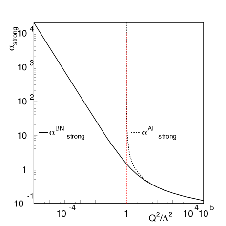
Figure 3: The figure Pancheri et al. (2014) shows the expression for $\alpha_{s}$ from Eq. (26) and its comparison with the asymptotic freedom expression, for the case $N_{f}=3$ and $\Lambda=$100 MeV.

Comparison of the above expression with data from Jade, LEPII and LHC Khachatryan et al. (2015) is seen in Fig. 4.

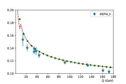
Figure 4: The expression for $\alpha_{s}$ as proposed in Eq. (26) is compared with experimental data (green stars) Khachatryan et al. (2015). The red dashes correspond to $\Lambda=100$ MeV and values of $N_{f}$ depending on the opening of the energy threshold, the green dots are for $N_{f}=5$. The gap corresponds to the threshold $N_{f}=4\rightarrow 5$.

IV.2 Limiting behaviour of $\alpha_{s}$

As discussed in Sec(IV), the simplest & most economical hypothesis for a confining $\alpha_{s}(Q^{2})$ in consonance at the same time with asymptotic freedom (AF) [at leading order] is given by

$$\alpha_{s}(Q^{2})=\frac{1}{ln[1+(\frac{Q^{2}}{\Lambda^{2}})^{b_{o}}]},$$ (27)

In an effort to find the renormalization group (RG) $\beta$- function that corresponds to Eq.(27), we can first write

$$\frac{1}{\alpha}=ln(1+\eta);\eta=(\frac{Q^{2}}{\Lambda^{2}})^{b_{o}},$$ (28)

and then write its derivative w.r.t. $\eta$ to read

$$\frac{d\alpha}{dln\eta}=\eta\frac{d\alpha}{d\eta}=-\alpha^{2}\frac{\eta}{1+\eta}$$ (29)

$$=-\alpha^{2}[1-\frac{1}{1+\eta}]=-\alpha^{2}[1-e^{-1/\alpha}]$$ (30)

having put $\alpha_{s}=\alpha$, for simplicity. Let us define $ln\eta=b_{o}t$. Then, with the standard definition of the RG beta function,

$$\frac{d\alpha}{dt}=\beta(\alpha),$$ (31)

corresponding to Eq.(27) reads

$$\beta(\alpha)=-b_{o}\alpha^{2}[1-e^{-1/\alpha}].$$ (32)

We note the following pleasing features of this beta function:

$${\rm(i):}\ \beta(\alpha)<0$$ (33)

$${\rm(ii):}\ \beta\to-b_{o}\alpha^{2}\ {\rm for}\ \alpha<<1;{\rm UV\ region}$$ (34)

$${\rm(iii)}\ \beta\to-b_{o}\alpha\ {\rm for}\ \alpha>>1;{\rm IR\ region}$$ (35)

. (36)

It may be of further interest to note that the dielectric function $\epsilon=n^{2}$, where $n$ is the refractive index, defined as usual

$$\alpha=\frac{1}{\epsilon}=\frac{1}{n^{2}},$$ (37)

the “beta-function” corresponding to $n$, the refractive index in this model, has a scaling property.

$$\frac{dn}{dt}=-\frac{\alpha^{-3/2}}{2}\frac{d\alpha}{dt}\equiv\ {\bar{\beta}}(n)$$ (38)

$${\bar{\beta}}(n)=\frac{b_{o}}{2}[\frac{1-e^{-n^{2}}}{n}]$$ (39)

Thus

$${\bar{\beta}}(n)\to(\frac{b_{o}}{2})n\to 0\ {\rm for}\ n\to 0\ {\rm IR\ region};$$ (40)

$${\bar{\beta}}(n)\to(\frac{b_{o}}{2})\frac{1}{n}\to 0\ {\rm for}\ n\to\infty\ {\rm UV\ region}.$$ (41)

Hence, in this model, ${\bar{\beta}}(n)$ tends to zero both in the IR & the UV regions, always remaining positive within the finite domain. Moreover, it has an asymptotic $n\leftrightarrow 1/n$ symmetry as one goes from the IR to the UV region.

$${\bar{\beta}}(n)\leftrightarrow{\bar{\beta}}(1/n)\ {\rm as}\ n\to 0.$$ (42)

This interesting symmetry appears to be a duality between strong and weak coupling similar to that conjectured from ADS/CFT Tan (2000); Brower et al. (2009).

It should also be noted that as ${\bar{\beta}}(n)$ goes to zero both for $n\to 0$ as well as $n\to\infty$, it has a maximum. Setting the derivative with respect to $n$ equal zero at $n={\bar{n}}$ in Eq.(38), we find the transcendental equation for ${\bar{n}}$:

$$e^{-{\bar{n}}^{2}}=\frac{1}{[1+2{\bar{n}}^{2}]},$$ (43)

whose numerical solution is

$$[{\bar{\beta}}(n)]^{2}\approx\ 1.275\ \ {\rm that\ corresponds\ to}\ {\bar{\alpha}}\approx\ 0.784,$$ (44)

remarkably similar to Gribov’s critical coupling for $SU(3)_{c}$, (see, Eq.(3) on page 344 of Gribov (2002)):

$$\alpha_{c}=\frac{2}{3-(1/3)}=\frac{3}{4}$$ (45)

According to Gribov, the critical coupling above ($\alpha_{s}=3/4$ for $SU(3)_{c}$) makes the color Coulomb potential between two colored quarks $U(r)=(4/3)(\hbar c)(\alpha_{s}/r)$ to take on the magic value $(\hbar c)/r$, exactly the value in QED when the nuclear charge $Z=137$ so that $Z\alpha_{QED}=1$ renders a nucleus unstable to decay into an ion with nuclear charge $Z=136$ and a positron. In QCD, according to Gribov, when $\alpha_{s}$ becomes $3/4$ (or, higher) the ($q\bar{q}$) state manifests itself as a colorless meson.

V Gribov dynamics with singular $\alpha_{s}(Q^{2})$

In the collection of papers [See Gribov (2002): Collected Works, specially Chapter IV in the book, “Gauge Theories & Quark Confinement”], Gribov writes down a set of equations for the quark Green’s function. He assumes that there exists an IR region where $\alpha_{s}>\alpha_{critical}$. Essentially, his work is focussed on an IR “frozen” $\alpha_{s}$ above the critical value. [See, his Eq.(92) in Chapter IV]. This is sufficient for him to obtain a phase transition, spontaneous breakdown of the chiral limit, the pion Goldstone modes etc. Gotsman and Levin (2021) A tour de force indeed.
What we would like to do is to go beyond and ask the question: what happens for a non-frozen, IR singular but integrable $\alpha_{s}$ of the type discussed in the Introduction? This interesting region is not covered by Gribov. Let us condense the argument. Gribov defines the couplings (Warning: the $\beta$ below is not the usual $\beta$ such as in the previous section)

$$\beta=1-g;\ g=\frac{4\alpha_{s}}{3\pi},$$ (46)

with $g>g_{c}$. Since his $g$ never gets close to 1, $\beta$ never hits zero. But look at his dynamical equations for the quark Green’s function [below $A_{\mu}$ is not the vector potential but is dynamically generated]:

$$[\frac{\partial}{\partial q_{\mu}}-A^{\mu}(q)]G^{-1}(q)=0;\ A^{\mu}(q)=[\frac{\partial}{\partial q_{\mu}}G^{-1}(q)]G(q)$$ (47)

and [with derivatives understood to be with respect to $q_{\mu}$]

$$\partial^{\mu}A_{\mu}(q)=-\beta(q)A_{\mu}(q)A^{\mu}(q).$$ (48)

For an IR singular $g$, $\beta$ can become zero (or even negative), cases not considered by Gribov. But when $\beta(q=q_{o})=0$, the rhs of Eq.(48) is zero, it appears that one has an interesting chiral invariant phase with $m(q_{o})$ driven to zero. However, this value is unstable. All we can say for the moment is that it looks very attractive, exciting and needs further investigation. For example, the quark mass in the IR region seems to inherit power law growth -an anomalous dimension- given by $b_{o}$.

VI Dispersion relation & a sum rule for the color refractive index

To go beyond a specific model and discuss the general case, the time honored approach is to employ analyticity and write a dispersion relation for $\alpha_{s}(s)$ with a right-hand branch cut for $s\geq 0$; see: Srivastava et al. (2001); Milton and Solovtsov (1997); Solovtsov and Shirkov (1999); Shirkov and Solovtsov (2007); Srivastava et al. (2009); Malaspina et al. (2024). In these previous works, dispersion relations for $\alpha_{s}$ or for $\epsilon$ were employed, both requiring one subtraction. Here we employ a dispersion relation for the color refractive index $n(s)=\sqrt{\epsilon(s)}=1/\sqrt{\alpha_{s}(s)}$, that should have the same domain of analyticity as $\alpha_{s}$ provided in the space-like region ($s=-Q^{2}<0$), $\alpha_{s}(Q^{2})$ does not vanish -a natural requirement for a coupling constant. Also, such a dispersion relation should require no subtraction under the hypothesis that (i) $\alpha_{s}(0)$ is either frozen (that is, it is a finite constant) or it diverges so that, $n(0)$ is finite or zero and (ii) for large $s$, asymptotic freedom prevails and thus $\Im m\ n(s)\to 0^{-}$ as $s\to\infty$.
Let us consider the refractive index $n(Q^{2})$ in the space-like region $s=-Q^{2}<0$. Normalizing it at the QCD scale $Q^{2}=\Lambda^{2}$, we have

$$n(Q^{2})=n(\Lambda^{2})+\frac{(\Lambda^{2}-Q^{2})}{\pi}\int_{o}^{\infty}\frac{ds\ \Im m\ n(s)}{(s+Q^{2})(s+\Lambda^{2})};$$

$$(\Im m\ n(s)<0;s>0);$$

$${\rm Thus:}\ n(Q^{2}>\Lambda^{2})>n(\Lambda^{2})$$

$$\&\ \alpha_{s}(Q^{2}>\Lambda^{2})<\alpha_{s}(\Lambda^{2});{\rm(asymptotic\ freedom)};$$

$${\rm In\ the\ IR\ region:}\ n(Q^{2}<\Lambda^{2})<n(\Lambda^{2})$$

$$\&\ \alpha_{s}(Q^{2}<\Lambda^{2})>\alpha_{s}(\Lambda^{2}).$$ (49)

Eq.(VI) is satisfactory in that the fall-off of $\alpha_{s}(Q^{2})$ for large $Q^{2}$ makes asymptotic freedom evident and its rise in the IR region ($Q^{2}<<\Lambda^{2}$) bodes well for reaching or, even overreaching, the Gribov critical value $\alpha_{s}(Q^{2}<\Lambda^{2})=3/4$, as discussed in the last section.
If indeed $n(0)=0$ (that is $\alpha_{s}(0)\to\infty$), then we have the sum rule

$$n(\Lambda^{2})=\frac{\Lambda^{2}}{\pi}\int_{o}^{\infty}\frac{ds\ [-\Im m\ n(s)]}{s(s+\Lambda^{2})}$$ (50)

To delineate further between a finite versus a divergent $\alpha_{s}(0)$, we show that only a divergent $\alpha_{s}(0)$ is consistent with the asymptotic duality for $\bar{\beta}(Q^{2})$, that was discussed earlier through a specific model - see Sec.(LABEL:alphass). The essential ingredient in obtaining the sought after asymptotic duality $\bar{\beta}_{IR}(Q^{2})\leftrightarrow\bar{\beta}_{UV}$ as $n\leftrightarrow 1/n$ is that $n_{IR}(Q^{2})$ vanish as a power-law $(Q^{2}/\Lambda^{2})^{q}$ as $Q^{2}\to 0$; only then, it can be matched with its AF logarithmic behavior. While the argument is more general, for simplicity we shall show it here only for the lowest perturbative order:

$$n_{IR}(Q^{2})\equiv n_{o}(\frac{Q^{2}}{\Lambda^{2}})^{q};$$

$$\bar{\beta}_{IR}=q\ n;(i);$$

$$n_{UV}(Q^{2})\equiv n_{\infty}[ln(\frac{Q^{2}}{\Lambda^{2}})]^{1/2};$$

$$\bar{\beta}_{UV}=(\frac{n_{\infty}^{2}}{2})\times(\frac{1}{n})=(\frac{b_{o}}{2})\times\frac{1}{n};(ii);$$

$${\rm Thus,\ equality\ between\ (i)\ and\ (ii)\ implies}:q=\frac{b_{o}}{2};$$ (51)

exactly as we found in Eqs.(40 & 42) for the specific model considered therein.

VII Conclusions

We have approached the infrared region in QCD, both in the continuum and the zero momentum point. After recapitulating previous work in QED in a formalism developed by Bruno Touschek which had been applied to investigate a zero momentum mode in Abelian gauge theories, we have extended Touschek’s approach to make the ansatz that could lead to a cut-off in impact parameter space in parton-parton collisions and shed light on the origin of the forward peak in hadronic collisions.

Breaking with tradition, we have considered dispersion relations for the color refractive index $n(s)=\sqrt{\epsilon(s)}=1/\sqrt{\alpha_{s}(s)}$ -for which no subtractions are needed- and a sum rule was derived for a divergent (but integrable $\alpha_{s}$ Grau et al. (1999)). It was also deduced that under the same hypothesis, an asymptotic duality ($n\leftrightarrow 1/n$) exists that in addition guarantees the integrability condition previously assumed in reference Grau et al. (2009). While our explicit expressions have been written down for 1-loop, the reader is encouraged to extend the formalism to higher loops.

We thank Fabrizio Palumbo, Simone Pacetti, L. Pierini and A. Grau for their contribution to discussions and interest in this problem.

References

- Amaldi et al. (1973) U. Amaldi et al., Phys. Lett. B 43, 231 (1973).
- Yodh et al. (1972) G. B. Yodh, Y. Pal, and J. S. Trefil, Phys. Rev. Lett. 28, 1005 (1972).
- Bartoli et al. (1970) B. Bartoli, B. Coluzzi, F. Felicetti, V. Silvestrini, G. Goggi, D. Scannicchio, G. Marini, F. Massa, and F. Vanoli, Nuovo Cim. A 70, 615 (1970).
- Aubert et al. (1974) J. J. Aubert et al. (E598), Physical Review Letters 33, 1404 (1974).
- Augustin et al. (1974) J. E. Augustin et al. (SLAC-SP-017), Physical Review Letters 33, 1406 (1974), [Adv. Exp. Phys.5,141(1976)].
- Bacci et al. (1974) C. Bacci et al., Physical Review Letters 33, 1408 (1974), [Erratum: Physical Review Letters33,1649(1974)].
- De Rujula and Glashow (1975) A. De Rujula and S. L. Glashow, Phys. Rev. Lett. 34, 46 (1975).
- Fagundes et al. (2015) D. A. Fagundes, A. Grau, G. Pancheri, Y. N. Srivastava, and O. Shekhovtsova, Phys. Rev. D 91, 114011 (2015), eprint 1504.04890.
- Amaldi et al. (1971) U. Amaldi et al., Phys. Lett. B 36, 504 (1971).
- Godbole et al. (2005) R. M. Godbole, A. Grau, G. Pancheri, and Y. N. Srivastava, Phys. Rev. D 72, 076001 (2005), eprint hep-ph/0408355.
- Pancheri and Srivastava (2017) G. Pancheri and Y. N. Srivastava, Eur. Phys. J. C 77, 150 (2017), eprint 1610.10038.
- Achilli et al. (2011) A. Achilli, R. M. Godbole, A. Grau, G. Pancheri, O. Shekhovtsova, and Y. N. Srivastava, Phys. Rev. D 84, 094009 (2011), eprint 1102.1949.
- Bloch and Nordsieck (1937) F. Bloch and A. Nordsieck, Phys. Rev. 52, 54 (1937).
- Etim et al. (1967) G. E. Etim, G. Pancheri, and B. Touschek, Nuovo Cim. B 51, 276 (1967).
- Durand and Pi (1988) L. Durand and H. Pi, Phys. Rev. D 38, 78 (1988).
- Pancheri-Srivastava and Srivastava (1977) G. Pancheri-Srivastava and Y. Srivastava, Phys. Rev. D15, 2915 (1977).
- Jenkovszky (2023) L. Jenkovszky, Acta Phys. Polon. Supp. 16, 33 (2023).
- Khoze et al. (2018) V. A. Khoze, A. D. Martin, and M. G. Ryskin, Phys. Lett. B 784, 192 (2018), eprint 1806.05970.
- Luna et al. (2024) E. G. S. Luna, M. G. Ryskin, and V. A. Khoze, Phys. Rev. D 110, 014002 (2024), eprint 2405.09385.
- Pancheri et al. (2014) G. Pancheri, D. A. Fagundes, A. Grau, O. Shekhovtsova, and Y. N. Srivastava, in International Conference on the Structure and the Interactions of the Photon (2014), eprint 1403.8050.
- Ryskin et al. (2009) M. G. Ryskin, A. D. Martin, and V. A. Khoze, Eur. Phys. J. C 60, 249 (2009), eprint 0812.2407.
- Fagundes et al. (2013) D. A. Fagundes, A. Grau, S. Pacetti, G. Pancheri, and Y. N. Srivastava, Phys. Rev. D 88, 094019 (2013), eprint 1306.0452.
- Jenkovszky et al. (2024) L. Jenkovszky, R. Schicker, and I. Szanyi, Universe 10, 208 (2024), eprint 2406.01735.
- Fagundes et al. (2016) D. A. Fagundes, L. Jenkovszky, E. Q. Miranda, G. Pancheri, and P. V. R. G. Silva, Int. J. Mod. Phys. A 31, 1645022 (2016).
- Antchev et al. (2019) G. Antchev et al. (TOTEM), Eur. Phys. J. C 79, 103 (2019), eprint 1712.06153.
- Palumbo (1983) F. Palumbo, Phys. Lett. B 132, 165 (1983).
- Palumbo and Pancheri (1984) F. Palumbo and G. Pancheri, Phys. Lett. B 137, 401 (1984).
- Weinberg (1965) S. Weinberg, Phys. Rev. 140, B516 (1965).
- Pancheri-Srivastava (1973) G. Pancheri-Srivastava, Phys. Lett. B 44, 109 (1973).
- Dokshitzer et al. (1978) Y. L. Dokshitzer, D. Diakonov, and S. I. Troian, Phys. Lett. B 79, 269 (1978).
- Parisi and Petronzio (1979) G. Parisi and R. Petronzio, Nucl. Phys. B 154, 427 (1979).
- Curci et al. (1979) G. Curci, M. Greco, and Y. Srivastava, Phys. Rev. Lett. 43, 834 (1979).
- Hayrapetyan et al. (2024) A. Hayrapetyan et al. (CMS) (2024), eprint 2409.17770.
- Grau et al. (1999) A. Grau, G. Pancheri, and Y. N. Srivastava, Phys. Rev. D 60, 114020 (1999), eprint hep-ph/9905228.
- Navas et al. (2024) S. Navas et al. (Particle Data Group), Phys. Rev. D 110, 030001 (2024).
- Khachatryan et al. (2015) V. Khachatryan et al. (CMS), Eur. Phys. J. C 75, 186 (2015), eprint 1412.1633.
- Tan (2000) C.-I. Tan, in 30th International Symposium on Multiparticle Dynamics (2000), pp. 105–110, eprint hep-ph/0102127.
- Brower et al. (2009) R. C. Brower, M. Djuric, and C.-I. Tan, JHEP 07, 063 (2009), eprint 0812.0354.
- Gribov (2002) V. Gribov, Gauge theories and quark confinement (PHASIS, Moscow, 2002).
- Gotsman and Levin (2021) E. Gotsman and E. Levin, Phys. Rev. D 103, 014020 (2021), eprint 2009.12218.
- Srivastava et al. (2001) Y. Srivastava, S. Pacetti, G. Pancheri, and A. Widom, eConf C010430, T19 (2001), eprint hep-ph/0106005.
- Milton and Solovtsov (1997) K. A. Milton and I. L. Solovtsov, Phys. Rev. D 55, 5295 (1997), eprint hep-ph/9611438.
- Solovtsov and Shirkov (1999) I. L. Solovtsov and D. V. Shirkov, Theor. Math. Phys. 120, 1220 (1999), eprint hep-ph/9909305.
- Shirkov and Solovtsov (2007) D. V. Shirkov and I. L. Solovtsov, Theor. Math. Phys. 150, 132 (2007), eprint hep-ph/0611229.
- Srivastava et al. (2009) Y. N. Srivastava, O. Panella, and A. Widom, Int. J. Mod. Phys. A 24, 1097 (2009), eprint 0811.3293.
- Malaspina et al. (2024) R. Malaspina, L. Pierini, O. Shekhovtsova, and S. Pacetti, Particles 7, 780 (2024), URL https://doi.org/10.3390/particles7030045.
- Grau et al. (2009) A. Grau, R. M. Godbole, G. Pancheri, and Y. N. Srivastava, Phys. Lett. B 682, 55 (2009), eprint 0908.1426.