Galaxy Tomography with the Gravitational Wave Background
from Supermassive Black Hole Binaries

Abstract

The detection of a stochastic gravitational wave background by pulsar timing arrays suggests the presence of a supermassive black hole binary population. Although the observed spectrum generally aligns with predictions from orbital evolution driven by gravitational wave emission in circular orbits, there is a discernible preference for a turnover at the lowest observed frequencies. This turnover could indicate a significant hardening phase, transitioning from early environmental influences to later stages predominantly influenced by gravitational wave emission. In the vicinity of these binaries, the ejection of stars or dark matter particles through gravitational three-body slingshots efficiently extracts orbital energy, leading to a low-frequency turnover in the spectrum. By analyzing the NANOGrav 15-year data, we assess how the gravitational wave spectrum depends on the initial inner galactic profile prior to disruption by binary ejections, accounting for a range of initial binary eccentricities. Our findings suggest a parsec-scale galactic center density around $\displaystyle 10^{6}\,M_{\odot}/\textrm{pc}^{3}$ across most of the parameter space, offering insights into the environmental effects on black hole evolution and combined matter density near galaxy centers.

I Introduction

Recent advances by pulsar timing arrays (PTAs), leveraging precise measurements of timing residuals within a galactic-scale detector, have ushered in a new era of stochastic gravitational wave background (SGWB) detection. The SGWB, defined by a superposition of incoherent gravitational waves (GWs), initially emerged as a common-spectrum process [1, 2, 3, 4]. Subsequent data provided robust evidence of a quadrupolar correlation function [5, 6, 7, 8], famously known as the Hellings-Downs curve [9], further affirming the SGWB’s presence and characteristics.

The observed spectrum of the SGWB is consistent with expectations for a population of supermassive black hole binaries (SMBHBs), dominated by binaries with comparable mass ratios, total masses in the range of $\displaystyle 10^{9.2-10.4}\,M_{\odot}$, and redshifts from $\displaystyle 0.15$ to $\displaystyle 0.9$ [10, 11], where $\displaystyle M_{\odot}$ represents the solar mass. Although the spectrum is consistent with a steady spectral slope driven by GW emission from circular binaries, it also suggests a low-frequency turnover [10, 12]. This feature implies an acceleration in the rate of orbital hardening, offering a potential solution to the final parsec problem [13, 14]. Possibilities include interactions with environmental factors—such as gas [15, 16], stars [17], and dark matter (DM) [18]—and the impact of significant initial orbital eccentricities [19, 20, 21].

An intriguing aspect of environmental interactions involves the role of stars and particle DM, which are noted for their potentially high density in galactic centers (GCs) [22, 23, 24]. Both stars and DM can be expelled from the system through gravitational slingshots during encounters with binary components, thereby extracting orbital energy [17]. This process involves three-body scattering, where the energy extraction efficiency is significantly higher than that of two-body dynamical friction [25], especially when the binary components have comparable masses and are sufficiently close. Such three-body slingshot interactions can substantially alter the density profile of the GC, particularly flattening the inner distribution [18, 26]. This underscores the importance of considering the co-evolution of the density profile and the binary orbit. A pivotal study by Ref. [27] demonstrates that the orbital hardening rate observed in N-body simulations can be effectively approximated by results from scattering experiments [17] within environments characterized by the GC distribution at the SMBHB influence radius [28] prior to disruption. In this study, we examine the impact of initial GC density profiles and SMBHB eccentricities on the SGWB spectrum, utilizing NANOGrav’s 15-year dataset to constrain the parameter space of these two factors.

II Binary Hardening by Three-body Scattering

The SGWB emanating from SMBHBs constitutes an incoherent superposition of signals from individual sources. The spectrum of this background is delineated by the characteristic strain, $\displaystyle h_{c}(f)$, as follows [29, 19]:

$$h_{c}^{2}(f)=\frac{4G}{c^{2}\pi f}\int{\rm d}z{\rm d}M{\rm d}q\frac{{\rm d}^{3}\eta}{{\rm d}z{\rm d}M{\rm d}q}\frac{{\rm d}E_{\mathrm{GW}}}{{\rm d}f_{s}},$$ (1)

where $\displaystyle G$ represents the gravitational constant, and $\displaystyle c$ denotes the speed of light. The GW frequency emitted in the source frame is denoted by $\displaystyle f_{s}$, and $\displaystyle f=f_{s}/(1+z)$, incorporating the redshift factor $\displaystyle z$. The comoving volumetric number density of SMBHBs, $\displaystyle\mathrm{d}^{3}\eta/(\mathrm{d}z\,\mathrm{d}M\,\mathrm{d}q)$, depends on the redshift $\displaystyle z$, the total binary mass $\displaystyle M$, and the mass ratio $\displaystyle q\leq 1$. The GW emission spectrum from a binary, $\displaystyle\mathrm{d}E_{\mathrm{GW}}/\mathrm{d}\ln f_{s}$, is expressed in the context of a circular orbit as follows [30]:

$$\frac{{\rm d}E_{\mathrm{GW}}}{{\rm d}f_{s}}\Big{|}^{e=0}=-\frac{{\rm d}t}{{\rm d}a}\frac{64}{15}\frac{\pi^{8/3}}{c^{5}}G^{8/3}M^{11/3}f_{s}^{5/3}\frac{q^{2}}{(1+q)^{4}}.$$ (2)

Here, $\displaystyle a$ represents the semi-major axis of the orbit, adhering to Kepler’s law $\displaystyle a^{3}=GM/(2\pi f_{\rm orb})^{2}$, where the orbital frequency $\displaystyle f_{\rm orb}=f_{s}/2$ for circular orbits. The orbital hardening process, denoted by $\displaystyle{\rm d}a/{\rm d}t\equiv\Sigma_{i}{\rm d}a/{\rm d}t|_{i}$, with the index $\displaystyle i$ encompassing various sources of hardening [31, 32, 33, 34], is crucial for binary evolution. The evolution of the semi-major axis due solely to GW emission in circular orbits is described as follows [35]:

$$\frac{{\rm d}a}{{\rm d}t}\Big{|}_{\rm GW}^{e=0}=-\frac{64}{5}\frac{G^{3}M^{3}}{c^{5}a^{3}}\frac{q}{(1+q)^{2}},$$ (3)

leading to a characteristic strain $\displaystyle h_{c}\propto f^{-2/3}$. Eccentric orbits lead to enhanced GW emission over a range of frequencies, as detailed in the Supplemental Material. Consequently, a turnover in the spectrum at lower frequencies is possible before the orbit undergoes circularization through GW emission [19].

In GCs, SMBHBs form within a background of stars and particle DM, once their separation falls below the influence radius, $\displaystyle r_{i}$. This radius is defined as the distance at which the total enclosed mass of stars and DM equals twice the mass of the SMBHB [28]. Given their substantial mass disparity with the SMBHB, both stars and DM particles act effectively as test particles. Each may undergo multiple gravitational encounters with one of the black holes (BHs) until it gains sufficient kinetic energy to be ejected. This three-body slingshot process becomes efficient as the semi-major axis $\displaystyle a$ approaches the hardening radius, defined as $\displaystyle a_{h}\equiv r_{i}q/(4(1+q)^{2})$ [17]. The rate of orbital hardening due to three-body scattering (3BS), averaged over a background of particles with matter density $\displaystyle\rho$ and velocity dispersion $\displaystyle\sigma$, is given by [17]:

$$\frac{{\rm d}a}{{\rm d}t}\Big{|}_{\text{3BS}}=-HG\frac{\rho}{\sigma}a^{2},$$ (4)

where $\displaystyle H$ is a dimensionless coefficient typically ranging from $\displaystyle 15$ to $\displaystyle 20$, as observed in scattering experiments [17]. It is important to note that three-body scattering is fundamentally distinct from two-body dynamical friction [25, 36, 37, 38, 39] and becomes more dominant after entering the hardening radius. Assuming a constant $\displaystyle\rho/\sigma$ ratio over time, the spectral evolution for circular orbits follows $\displaystyle h_{c}\propto f$. Note that three-body scatterings tend to increase the eccentricity on average [17], in contrast to the effects of GW emission.

Historically, the three-body slingshot process was thought to result in stalled orbital evolution by expelling background stars and depleting a specific phase-space region known as the loss cone. This led to what is known as the final parsec problem [13]. However, N-body simulations [40, 41, 42] have shown that merger-induced triaxiality can efficiently repopulate the loss cone [43].

These simulations also reveal that two initial DM profiles, each centered around a BH with peak densities at the center, will merge and flatten into a single core profile following the merger [18, 26, 44]. This underscores the need for comprehensive simulations that simultaneously address the co-evolution of the SMBHB orbit and the density profile. Further analysis comparing results from scattering experiments [17] with N-body simulation outcomes [42] demonstrates that predictions of orbital evolution can closely align with Eq. (4), assuming that $\displaystyle\rho/\sigma$ remains constant, determined by the initial profile at the SMBHB’s influence radius, $\displaystyle r_{i}$ [27]. This statement is supported by observations that the total mass ejected during SMBHB evolution is approximately of the order of $\displaystyle M$ [17, 45, 18, 46], primarily distributed within the influence radius at the onset. During simulations, the loss cone at this radius remains fully populated, driven by the efficient diffusion of particles.

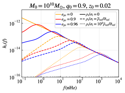
Figure 1: Examples of the SGWB spectrum derived from an SMBHB population modeled as delta functions in the space of $\displaystyle(M,q,z)$, specifically, $\displaystyle{\rm d}^{3}\eta/({\rm d}z{\rm d}M{\rm d}q)=\delta(M-M_{0})\delta(z-z_{0})\delta(q-q_{0})\,{\rm Mpc^{-3}}$. The constant parameters $\displaystyle(M_{0},z_{0},q_{0})$ are indicated at the top. All scenarios initiate the evolution of the semi-major axis $\displaystyle a$ and contribute to GW emission starting at $\displaystyle 1$ pc, with the eccentricity $\displaystyle e_{\rm pc}$ defined at this separation. Colors indicate different $\displaystyle e_{\rm pc}$ values, while line styles represent different $\displaystyle\rho_{i}/\sigma_{i}$ for three-body scattering, with $\displaystyle\bar{\rho}_{\rm ref}\equiv 10^{5}\,M_{\odot}/\text{pc}^{3}$ and $\displaystyle\bar{\sigma}_{\rm ref}\equiv 10^{-3}\,c$.

By combining Eq. (3) and Eq. (4), the GW spectrum is revealed to exhibit two distinct phases: one at low frequencies, predominantly shaped by three-body scattering, and another at high frequencies, primarily determined by GW emission. The transition between these phases is marked by a turnover frequency in the source frame [20]:

$$\begin{split}f_{t}&=\pi^{-1}\left(\frac{5c^{5}}{64}\frac{(1+q)^{2}}{q}\frac{\rho_{i}}{\sigma_{i}}H\right)^{3/10}G^{-1/10}M^{-2/5}\\ &\approx 2.8\,\text{nHz}\,\left(\frac{(1+{q})^{2}}{{q}}\frac{{\rho}_{i}/\bar{\rho}_{\rm ref}}{{\sigma}_{i}/\bar{\sigma}_{\rm ref}}\frac{H}{18}\right)^{3/10}\left(\frac{M}{10^{10}M_{\odot}}\right)^{-2/5},\end{split}$$ (5)

Here, we define $\displaystyle\bar{\rho}_{\rm ref}\equiv 10^{5}\,M_{\odot}/\text{pc}^{3}\approx 3.8\times 10^{6}\,c^{-2}\,\text{GeV}/\text{cm}^{3}$ and $\displaystyle\bar{\sigma}_{\rm ref}\equiv 10^{-3}c$. Figure 1 presents examples of the GW spectrum from an individual SMBHB across various parameter settings, demonstrating how the magnitude of three-body scattering and the initial binary eccentricity influence the spectral shape.

III Galaxy Tomography

The NANOGrav $\displaystyle 15$-year data indicates a slight preference for a turnover at low frequencies, particularly around $\displaystyle 4$ nHz [10, 12], suggesting deviations from the expected behavior of purely circular binaries driven by GW emission. Given that both eccentricity and star/DM-induced three-body scatterings can contribute to this turnover, we conduct a comprehensive survey of their joint parameter space.

We adopt a straightforward power-law distribution for the GC density profile prior to disruption, parameterized as follows:

$$\rho(r)=\rho_{\rm pc}\left(\frac{r}{1\,\text{pc}}\right)^{-\gamma},$$ (6)

where the reference radius $\displaystyle 1$ pc is set for our analysis, $\displaystyle\rho_{\mathrm{pc}}$ denotes the matter density normalization to be constrained, and $\displaystyle\gamma$ represents the radial slope of the profile. We explore values of $\displaystyle\gamma$ ranging from $\displaystyle 0$ to $\displaystyle 2.5$, consistent with the inner region of the Dehnen density profile family [47]. For each scenario, we first determine the influence radius $\displaystyle r_{i}$ by satisfying the condition $\displaystyle\textstyle\int_{0}^{r_{i}}\!\rho\,4\pi r^{2}dr=2M$ [28], and then calculate $\displaystyle\rho_{i}\equiv\rho(r_{i})$ using Eq. (6) and $\displaystyle\sigma_{i}\equiv\sigma(r_{i})=\sqrt{GM/r_{i}}$ via the virial theorem.

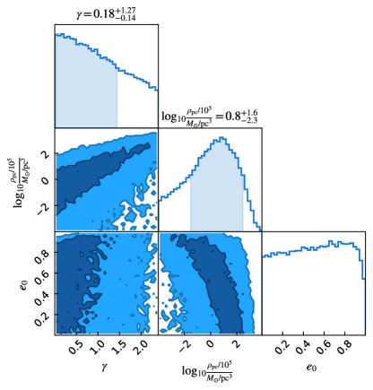
Figure 2: Posterior distribution of the parameters $\displaystyle(\log_{10}(\rho_{\rm pc}[M_{\odot}/\text{pc}^{3}]/10^{5}),\gamma)$ for the density profile prior to disruption and initial eccentricity $\displaystyle e_{0}$ from the lowest five frequency bins of the NANOGrav 15-year dataset. The $\displaystyle 1\,\sigma$ and $\displaystyle 2\,\sigma$ confidence regions are depicted in dark blue and light blue, respectively. The SMBHB population parameters used to produce the SGWB follow the fiducial ‘Phenom+Astro’ model from Ref. [10], without incorporating phenomenological environmental parameters, with normalization treated as a nuisance parameter based on astrophysical priors.

Our analysis targets include the initial eccentricity $\displaystyle e_{0}$, defined as occurring when the binary is formed at $\displaystyle a=r_{i}$, and the density profile parameters $\displaystyle\rho_{\rm pc}$ and $\displaystyle\gamma$. The distribution of SMBHB parameters, including total mass $\displaystyle M$, mass ratio $\displaystyle q$, and redshift $\displaystyle z$, follows the fiducial population model derived from NANOGrav’s astrophysical interpretations (fiducial ‘Phenom+Astro’ model without phenomenological environmental parameters) using holodeck [10]. The dominant contributions to the SGWB are expected from binaries with $\displaystyle\log_{10}(M/M_{\odot})\in(9.2,10.4)$, $\displaystyle q\in(0.5,0.8)$, and $\displaystyle z\in(0.15,0.9)$.

For each parameter combination of $\displaystyle(e_{0},\rho_{\rm pc},\gamma)$ and $\displaystyle(M,q,z)$, we compute the orbital and eccentricity evolution of the SMBHB, taking into account both GW emission and three-body scattering, as detailed in the Supplemental Material. We then derive the total SGWB spectrum by integrating over $\displaystyle(M,q,z)$. Finally, we assess the likelihood that the SGWB spectrum, generated from each set of parameters $\displaystyle(e_{0},\rho_{\rm pc},\gamma)$, matches the lowest five frequency bins, ranging from $\displaystyle 2$ to $\displaystyle 10$ nHz, of the NANOGrav 15-year data, which exhibit robust signal-to-noise ratios [5]. We treat the overall normalization of the SMBHB distribution as a nuisance parameter, assigning it a prior derived from astrophysical priors, as detailed in Supplemental Material.

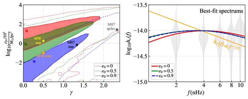
Figure 3: Left: Posterior distribution of the density profile parameters $\displaystyle(\log_{10}(\rho_{\rm pc}[M_{\odot}/\text{pc}^{3}]/10^{5}),\gamma)$ for three specific initial eccentricities: $\displaystyle e_{0}=0$ (blue), $\displaystyle 0.5$ (green), and $\displaystyle 0.9$ (red). The $\displaystyle 1\,\sigma$ and $\displaystyle 2\,\sigma$ confidence regions are depicted in darker shades and marked by dashed lines, respectively. Benchmark matter density profiles, including the star distribution in M87 (black star), the star core in the Milky Way (MW) (yellow star), a dark matter (DM) spike in M87 (gray dot), and a flattened DM core in the MW (orange dot), are presented for comparison, with detailed parameters provided in the text. Right: Best-fit SGWB spectrum with parameters $\displaystyle(\log_{10}(\rho_{\rm pc}[M_{\odot}/\text{pc}^{3}]/10^{5}),\gamma)=(1.3,0,0.08),(-0.09,0.06)$, and $\displaystyle(-1.9,0.27)$ for $\displaystyle e_{0}=0,0.5$, and $\displaystyle 0.9$, respectively, as indicated by the crosses $\displaystyle(\times)$ in the left panel with darker colors. The spectrum is shown against the lowest five frequency bins from the NANOGrav $\displaystyle 15$-year dataset [5].

In Fig. 2, we present the posterior distribution of the parameters $\displaystyle(e_{0},\log_{10}(\rho_{\rm pc}[M_{\odot}/\text{pc}^{3}]/10^{5}),\gamma)$. The results reveal that the $\displaystyle 1\,\sigma$ regions (dark blue) indicate the presence of three-body scatterings, with $\displaystyle\log_{10}(\rho_{\rm pc}[M_{\odot}/\text{pc}^{3}]/10^{5})$ estimated at $\displaystyle 0.8^{+1.7}_{-2.3}$. Variations in the SMBHB population distribution would only shift this best-fit region, adhering to the scaling relations from Eq. (5). There is an expected degeneracy between $\displaystyle e_{0}$ and $\displaystyle\rho_{\rm pc}$ [48, 49, 11, 50], where a higher $\displaystyle e_{0}$ corresponds to a lower required density. However, the $\displaystyle 1\,\sigma$ region indicates that when $\displaystyle\rho_{\rm pc}$ drops below $\displaystyle 10\,M_{\odot}/\text{pc}^{3}$, GW emission requires an extremely high initial eccentricity, $\displaystyle e_{0}>0.999$, to account for the turnover. This is because lower densities result in a larger $\displaystyle r_{i}$, and GW emission tends to circularize the orbit before it reaches the observed frequency range. The light blue regions represent the $\displaystyle 2\,\sigma$ confidence interval. The white region is excluded at the $\displaystyle 95\%$-confidence level, thereby setting an upper limit on $\displaystyle\rho_{\rm pc}$ as it would result in a turnover frequency inconsistent with the observational data.

In the left panel of Fig. 3, we present the posterior distribution for the density profile parameters ($\displaystyle\rho_{\rm pc},\gamma$) for specific initial eccentricities of $\displaystyle e_{0}=0,0.5,$ and $\displaystyle 0.9$. The contours generally follow approximately constant values of $\displaystyle\rho_{i}/\sigma_{i}$, as suggested by Eq. (5). The right panel of Fig. 3 presents the best-fit spectrum for various values of $\displaystyle e_{0}$. Distributions with smaller $\displaystyle\gamma$ values are preferred over steeper ones because larger $\displaystyle\gamma$ leads to a broader range of $\displaystyle\rho_{i}/\sigma_{i}$ across the SMBHB population parameters $\displaystyle(M,q)$, which in turn results in a wider distribution of the turnover frequency $\displaystyle f_{t}$ as defined in Eq. (5). This causes the spectrum to have a broader intermediate region, requiring a normalization factor higher than the fiducial value, making high-$\displaystyle\gamma$ cases less favored. A conservative upper limit on $\displaystyle\rho_{\rm pc}(\gamma)$ is established based on the $\displaystyle 95\%$ exclusion for $\displaystyle e_{0}=0$, since higher $\displaystyle e_{0}$ values lead to more stringent constraints.

For comparative purposes, we examine various benchmark star and DM profiles: the modelled stellar distribution in the nearby galaxy M87 with $\displaystyle\gamma=4/3$ and $\displaystyle\rho_{\rm pc}\approx 0.7\times 10^{5}\,M_{\odot}/\text{pc}^{3}$ [51] (black star); the Milky Way’s (MW) modelled core star distribution with $\displaystyle\gamma=1/2$ and $\displaystyle\rho_{\rm pc}\approx 1.8\times 10^{5}\,M_{\odot}/\text{pc}^{3}$ [52] (yellow star); a hypothetical DM spike in M87 with $\displaystyle\gamma=7/3$ and $\displaystyle\rho_{\rm pc}\approx 2.6\times 10^{6}\,M_{\odot}/\text{pc}^{3}$ [23], formed by an adiabatically growing central SMBH from an initial Navarro-Frenk-White distribution [22] (brown dot); and a hypothetical flattened DM spike in the MW with $\displaystyle\gamma=1/2$ and $\displaystyle\rho_{\rm pc}\approx 10^{4}\,M_{\odot}/\text{pc}^{3}$, formed as the BH grew from a low-mass seed [53] (orange dot). Interestingly, DM spikes are not favored in the hardening process because higher $\displaystyle\gamma$ values result in larger $\displaystyle r_{i}$ above $\displaystyle 1$ pc, leading to lower $\displaystyle\rho_{i}$. Conversely, the core-like star or DM distributions with $\displaystyle\gamma=1/2$ align with our best-fit regions. Lower $\displaystyle\gamma$ values are expected due to flattening by previous SMBHB mergers or reformation after a galaxy merger [53].

IV Discussion

In the vicinity of a binary BH, a test particle can extract orbital energy through multiple scatterings with each BH component. Within the PTA observation band, the three-body ejection process is significantly more efficient than two-body dynamical friction, particularly for comparable-mass binaries, leading to pronounced backreaction effects on the surrounding matter distribution. In this study, we explore the potential imprints that stars or particle DM surrounding SMBHBs could leave on the spectrum of the SGWB. Utilizing data from NANOGrav’s 15-year observation, we constrain the relevant parameter space. Our results support the existence of three-body scatterings with a reasonable density distribution prior to disruption (see the left panel of Fig. 2), primarily inferred from the low-frequency turnover in the SGWB spectrum, assuming no other dominant environmental influences are present. Continued monitoring with existing PTAs will provide improved constraints on the low-frequency turnover. Future observations from the Square Kilometre Array [54] and next-generation astrometry missions [55] are expected to provide significantly more precise spectral information [56], potentially elucidating the turnover.

Another potential source of environmental effects is a circumbinary disk around the SMBHB. If the GCs hosting SMBHBs are gas-rich and the binaries are accreting at the Eddington rate, the gas-driven hardening rate (conservatively choosing large values from Ref. [57]), could be comparable to three-body scatterings at separations below $\displaystyle 0.1$ pc for $\displaystyle M\sim 10^{10}\,M_{\odot}$ ($\displaystyle 2$ nHz). However, at these separations and lower the binary will decouple from the disk [58], thus mitigating disk-driven hardening. Furthermore, SMBHBs of this mass cannot be surrounded by gravitationally stable thin disks until closer to merger and massive self-gravitating disks must be employed [59, 60, 61].

To precisely determine the density profile, resolving the degeneracy with the initial eccentricity is essential. Potential strategies to determine SMBHB eccentricity include resolving individual binaries through either GW or electromagnetic observations [62, 63] and examining correlations among different frequency bins. This latter method is based on the observation that high eccentricity contributes to multiple integer multiples of frequency bins simultaneously [21]. Nevertheless, setting a stringent upper limit on the galactic center density distribution is feasible, as both additional environmental influences and nonzero orbital eccentricity tend to further elevate the turnover frequency.

The three-body slingshot mechanism considered in this study assumes that the test particles interact purely gravitationally, thus applying to both stars and cold, collisionless DM. If DM is the dominant density, the findings here could provide crucial insights into two longstanding questions: the identification of the particle nature of DM and the measurement of its density at galactic centers. Further investigations are needed to determine how DM models that extend beyond the test particle hypothesis—such as wave-like DM [38] or self-interacting DM [64, 65]—interact with binaries, particularly in terms of the applicability of three-body ejection or two-body dynamical friction. Notably, wave-like DM exhibits distinct behaviors depending on the binary separation scale and the boson mass [66, 67, 68, 69, 70, 71]. For a star-dominant distribution, such findings could reveal the star formation and relaxation rates near SMBHs in the galactic center, suggesting a density higher than previously expected [72, 20].

Authorship Contributions

This paper uses a decade’s worth of pulsar timing observations and is the product of the work of many people.

Y.C., L.S., and X.X. initiated the project and developed the core idea, with D.J.D. contributing to its development. Y.C., M.D., D.J.D., A.M., L.S., and X.X. participated in discussions, provided critical feedback, and shaped the research and analysis. Y.C. coordinated the project and wrote the manuscript. M.D. and X.X. developed the analysis code, created figures, and edited the text. D.J.D. offered guidance on the supermassive black hole binary population model and the holodeck code, wrote the discussion on the environmental effects from gas, and edited the text. A.Mi. provided guidance on the PTArcade code and the presentation of NANOGrav 15-year data.

G.A., A.A, A.M.A., Z.A., P.T.B., P.R.B., H.T.C., K.C., M.E.D, P.B.D., T.D., E.C.F, W.F., E.F., G.E.F., N.G.D., D.C.G., P.A.G., J.G., R.J.J., M.L.J., D.L.K., M.K., M.T.L., D.R.L., J.L., R.S.L., A.M., M.A.M., N.M., B.W.M., C.N., D.J.N., T.T.N., B.B.P.P., N.S.P., H.A.R., S.M.R., P.S.R., A.S., C.S., B.J.S.A., I.H.S., K.S., A.S., J.K.S., and H.M.W. developed timing models and ran observations for the NANOGrav 15 yr data set. Development of the holodeck population modeling framework was led by L.Z.K., with contributions from A.C-C., D.W., E.C.G., J.M.W., K.G., M.S.S., and S.C. PTArcade, which was used in this analysis, was mainly developed by A.Mi., with help from D.W., K.D.O., J.N., R.v.E., T.S., and T.T.

V Evolution of Eccentric Orbits

We investigate the orbital evolution of supermassive black hole binaries (SMBHBs) driven by both three-body ejection of stars and dark matter (DM), and gravitational wave (GW) emission. In addition to the formalism presented in the main text, our analysis incorporates eccentric orbits with evolving eccentricity. The coupled equations that govern the semi-major axis $\displaystyle a$ and eccentricity $\displaystyle e$ are as follows:

$$\begin{split}\frac{{\rm d}a(e,a)}{{\rm d}t}=&-\frac{64}{5}\frac{G^{3}M^{3}}{c^{5}a^{3}}\frac{q}{(1+q)^{2}}\frac{(1+\frac{73}{24}e^{2}+\frac{37}{96}e^{4})}{(1-e^{2})^{7/2}}-HG\frac{\rho_{i}}{\sigma_{i}}a^{2},\\ \frac{{\rm d}e(e,a)}{{\rm d}t}=&-\frac{304}{15}\frac{G^{3}M^{3}}{c^{5}a^{4}}\frac{q}{(1+q)^{2}}\frac{e(1+\frac{121}{304}e^{2})}{(1-e^{2})^{5/2}}+HK(e,a)G\frac{\rho_{i}}{\sigma_{i}}a.\end{split}$$ (S1)

The first terms on the right-hand side of these equations correspond to GW emission [30], while the second terms describe the effects of three-body ejections [17]. Here, $\displaystyle G$ denotes the gravitational constant, $\displaystyle M$ the total mass of the SMBHB, $\displaystyle q\leq 1$ the mass ratio of its components, and $\displaystyle\rho_{i}$ and $\displaystyle\sigma_{i}$ the matter density and velocity dispersion at the SMBHB influence radius $\displaystyle r_{i}$, respectively. The dimensionless parameters $\displaystyle H$ and $\displaystyle K$ represent the hardening and eccentricity growth rates, respectively, derived from scattering experiments. For hard binaries, $\displaystyle H$ values typically range from $\displaystyle 15$ to $\displaystyle 20$ [17]; in this study, we have fixed $\displaystyle H$ at $\displaystyle 18$. The function for $\displaystyle K$ is approximated by [17, 73, 74, 75]:

$$K(e,a)\approx 0.3e\left(1-e^{2}\right)^{0.6}\left(1+\frac{a}{0.2\,a_{h}}\right)^{-1},$$ (S2)

which becomes most effective when $\displaystyle a$ is within the hardening radius $\displaystyle a_{h}\equiv r_{i}q/(4(1+q)^{2})$.

Each evolutionary case begins at the influence radius, $\displaystyle r_{i}$, determined by solving the relation $\displaystyle\textstyle\int_{0}^{r_{i}}\!\rho\,4\pi r^{2}dr=2M$ [28] for a power-law distribution $\displaystyle\rho(r)=\rho_{\rm pc}(r/1\,\text{pc})^{-\gamma}$ prior to disruption. Consequently, $\displaystyle\rho_{i}\equiv\rho(r_{i})$ and $\displaystyle\sigma_{i}\equiv\sigma(r_{i})=\sqrt{GM/r_{i}}$ are calculated. The initial eccentricity, $\displaystyle e_{0}$, defined at $\displaystyle r_{i}$, serves as a fit parameter to be constrained.

We vary both the initial eccentricity, $\displaystyle e_{0}$, and the density profile parameters $\displaystyle(\rho_{\rm pc},\gamma)$. We then calculate the orbital evolution for the SMBHB with parameters $\displaystyle(M,q)$ from the determined $\displaystyle r_{i}$. The stochastic gravitational wave background (SGWB) spectrum is subsequently calculated by integrating over the SMBHB population parameters $\displaystyle(M,q,z)$, considering the density distribution $\displaystyle\mathrm{d}^{3}\eta/(\mathrm{d}z\,\mathrm{d}M\,\mathrm{d}q)$, as referenced in [29, 19, 76]:

$$h_{c}^{2}(f)=\frac{4G}{c^{2}\pi f}\int{\rm d}z{\rm d}M{\rm d}q\frac{{\rm d}^{3}\eta}{{\rm d}z{\rm d}M{\rm d}q}\frac{{\rm d}E_{\mathrm{GW}}}{{\rm d}f_{s}}\Big{|}_{f_{s}=(1+z)f}.$$ (S3)

In this calculation, we neglect Poisson fluctuations in the SMBHB distribution, which have a minor impact on the lowest frequency bins of the NANOGrav $\displaystyle 15$-year dataset [77, 78, 79, 80, 81].

The GW emission spectrum, $\displaystyle\mathrm{d}E_{\mathrm{GW}}/\mathrm{d}\ln f_{s}$, calculated at the source frame frequency $\displaystyle f_{s}$, includes contributions from various orbital frequencies $\displaystyle f_{\rm orb}^{n}=f_{s}/n$ for integer $\displaystyle n>0$. It is expressed as [30]:

$$\frac{{\rm d}E_{\mathrm{GW}}}{{\rm d}f_{s}}\Big{|}_{f_{s}=(1+z)f}=\sum_{n=1}^{+\infty}\frac{{\rm d}E_{\mathrm{GW}}^{n}/{\rm d}t}{n{\rm d}f_{\rm orb}^{n}/{\rm d}t}\Big{|}_{f_{\rm orb}^{n}=(1+z)f/n},$$ (S4)

where

$$\begin{aligned} \frac{{\rm d}E_{\mathrm{GW}}^{n}}{{\rm d}t}&=\frac{32G^{4}M^{5}}{5c^{5}a^{5}}\frac{q^{2}}{(1+q)^{4}}g(n,e),\\ \frac{{\rm d}f_{\rm orb}^{n}}{{\rm d}t}&=-\frac{3\sqrt{GM}}{4\pi a^{5/2}}\frac{{\rm d}a}{{\rm d}t}.\end{aligned}.$$ (S5)

The orbital frequency is related to $\displaystyle a$ via Kepler’s law $\displaystyle a^{3}=GM/(2\pi f_{\rm orb}^{n})^{2}$. The function $\displaystyle g(n,e)$, defined as

$$g(n,e) =\frac{n^{4}}{32}\bigg{[}\Big{\{}J_{n-2}(ne)-2eJ_{n-1}(ne)+\frac{2}{n}J_{n}(ne)+2eJ_{n+1}(ne)-J_{n+2}(ne)\Big{\}}^{2}$$ (S6)

$$+\left(1-e^{2}\right)\Big{\{}J_{n-2}(ne)-2J_{n}(ne)+J_{n+2}(ne)\Big{\}}^{2}+\frac{4}{3n^{2}}J_{n}^{2}(ne)\bigg{]},$$

converges to $\displaystyle g(2,0)=1$ for circular orbits. Here, $\displaystyle J_{n}$ denotes the Bessel function of the first kind of order $\displaystyle n$.

In practice, we employ several methods to enhance the efficiency of numerical computation. In Eq. (S4), we apply a cutoff to the summation over $\displaystyle n$, neglecting all contributions for $\displaystyle n>n_{\rm max}$, with $\displaystyle n_{\rm max}=3n_{\rm peak}(e_{\rm max})$. The value of $\displaystyle n_{\rm peak}(e)$ is given by [82]:

$$n_{\rm peak}(e)\approx 2\left(1+\sum_{k=1}^{4}c_{k}e^{k}\right)\,(1-e^{2})^{-3/2},$$ (S7)

where $\displaystyle c_{1}=-1.01678$, $\displaystyle c_{2}=5.57372$, $\displaystyle c_{3}=-4.9271$, and $\displaystyle c_{4}=1.68506$ and $\displaystyle e_{\rm max}$ represents the maximum eccentricity throughout the orbital evolution. Additionally, when $\displaystyle n_{\rm max}$ exceeds $\displaystyle 100$, we sum the contributions for $\displaystyle n>101$ using logarithmic steps (i.e., $\displaystyle n=101,102,104,108,\dots$) and implement numerical integration over $\displaystyle n$ using numpy.trapz.

VI Supermassive Black Hole Binary Population

This section details the semi-analytic SMBHB population model utilized in this study, characterized by the comoving volumetric number density of SMBHBs, $\displaystyle\mathrm{d}^{3}\eta/(\mathrm{d}z\,\mathrm{d}M\,\mathrm{d}q)$, alongside astrophysical priors on its normalization. To generate the initial SMBHB population before binary evolution, we use the holodeck code, following NANOGrav’s astrophysical interpretation paper [10]. However, we replaced the phenomenological environmental prescription [32, 10, 12, 83, 84] with the three-body scattering prescription detailed in Sec. V.

The semi-analytic model is predicated on galaxy merger rates, the SMBH-host galaxy relationship, and cosmological expansion, and is parameterized as follows [85, 86]:

$$\frac{\mathrm{d}^{3}\eta}{\mathrm{d}z\,\mathrm{d}M\,\mathrm{d}q}=\frac{\mathrm{d}^{3}\eta_{\text{gal-gal}}}{\mathrm{d}z\,\mathrm{d}m_{\star 1}\,\mathrm{d}q_{\star}}\frac{\mathrm{d}m_{\star 1}}{\mathrm{d}M}\frac{\mathrm{d}q_{\star}}{\mathrm{d}q},$$ (S8)

where $\displaystyle{\mathrm{d}^{3}\eta_{\text{gal-gal}}}/{(\mathrm{d}z\,\mathrm{d}m_{\star 1}\,\mathrm{d}q_{\star})}$ represents the volumetric galaxy merger rate density as a function of redshift $\displaystyle z$, the stellar mass of the primary galaxy $\displaystyle m_{\star 1}$, and the mass ratio of the galaxies $\displaystyle q_{\star}\leq 1$. The galaxy merger rate can be expressed [49]:

$$\frac{\mathrm{d}^{3}\eta_{\text{gal-gal}}}{\mathrm{d}z\,\mathrm{d}m_{\star 1}\,\mathrm{d}q_{\star}}=\frac{\Psi(m_{\star 1},z^{\prime})}{m_{\star 1}\ln(10)}\frac{P(m_{\star 1},q_{\star},z^{\prime})}{T_{\text{gal-gal}}(m_{\star 1},q_{\star},z^{\prime})}\frac{{\rm d}t}{{\rm d}z^{\prime}}.$$ (S9)

Here, $\displaystyle\Psi(m_{\star 1},z’)$ represents the galaxy stellar mass function (GSMF), $\displaystyle P(m_{\star 1},q_{\star},z’)$ denotes the galaxy pair fraction (GPF), and $\displaystyle T_{\text{gal-gal}}(m_{\star 1},q_{\star},z’)$ refers to the galaxy merger timescale (GMT). The variable $\displaystyle z’$ is defined as the advanced redshift satisfying $\displaystyle t(z)-t(z’)=T_{\text{gal-gal}}(z’)$, with the current epoch at $\displaystyle t(0)=13.79$ Gyr. The rate of change in cosmic time with respect to redshift, $\displaystyle{\rm d}t/{\rm d}z$, is calculated as $\displaystyle 1/((1+z)H(z))$, following the standard cosmological model where the Hubble parameter $\displaystyle H(z)=H_{0}\left[\Omega_{\Lambda}+(1+z)^{3}\Omega_{m}\right]^{1/2}$ with $\displaystyle H_{0}=67.4\,\mathrm{km}\,\mathrm{s}^{-1}\,\mathrm{Mpc}^{-1},\Omega_{m}=0.315$, and $\displaystyle\Omega_{\Lambda}=0.685$. The terms $\displaystyle{\mathrm{d}m_{\star 1}}/{\mathrm{d}M}$ and $\displaystyle{\mathrm{d}q_{\star}}/{\mathrm{d}q}$ are derived from the SMBH-host relation.

Below, we detail the relevant parameters in the semi-analytic model:

• Galaxy Stellar Mass Function (GSMF) $\displaystyle\Psi(m_{\star 1},z)$: This function describes the distribution of primary galaxy masses $\displaystyle m_{\star 1}$ at different redshifts $\displaystyle z$, following the Schechter function [87]:

  $$\Psi(m_{\star 1},z)=\ln(10)\Psi_{0}\left(\frac{m_{\star 1}}{M_{\psi}}\right)^{\alpha_{\psi}}\exp\left(-\frac{m_{\star 1}}{M_{\psi}}\right),$$ (S10)

  where

  $$\log_{10}\left(\Psi_{0}/\mathrm{Mpc}^{-3}\right) =\psi_{0}+\psi_{z}\cdot z,$$ (S11)

  $$\log_{10}\left(M_{\psi}/\mathrm{M}_{\odot}\right) =m_{\psi,0}+m_{\psi,z}\cdot z,$$

  $$\alpha_{\psi} =1+\alpha_{\psi,0}+\alpha_{\psi,z}\cdot z.$$

• Galaxy Pair Fraction (GPF) $\displaystyle P(m_{\star 1},q_{\star},z)$: This parameterizes the relative number of observable galaxy pairs to total galaxies, following [49]:

  $$P(m_{\star 1},q_{\star},z)=P_{0}\left(\frac{m_{\star 1}}{10^{11}M_{\odot}}\right)^{\alpha_{p}}(1+z)^{\beta_{p}}q_{\star}^{\gamma_{p}},$$ (S12)

  where

  $$\alpha_{p} =\alpha_{p,0}+\alpha_{p,z}\cdot z,$$ (S13)

  $$\gamma_{p} =\gamma_{p,0}+\gamma_{p,z}\cdot z.$$

• Galaxy Merger Timescale (GMT) $\displaystyle T_{\text{gal-gal}}(m_{\star 1},q_{\star},z)$: This provides the duration for two galaxies to merge, expressed as [49]:

  $$T_{\text{gal-gal}}(m_{\star 1},q_{\star},z)=T_{0}\left(\frac{m_{\star 1}}{10^{11}M_{\odot}/h}\right)^{\alpha_{t}}(1+z)^{\beta_{t}}q_{\star}^{\gamma_{t}},$$ (S14)

  where

  $$\alpha_{t} =\alpha_{t,0}+\alpha_{t,z}\cdot z,$$ (S15)

  $$\gamma_{t} =\gamma_{t,0}+\gamma_{t,z}\cdot z.$$

• SMBH–host relation: This assumes a one-to-one correspondence between galaxy pairs and SMBHBs as per Ref. [10], expressed as

  $$\log_{10}(M_{\text{BH}}/M_{\odot})=\mu+\alpha_{\mu}\log_{10}\left(\frac{M_{\text{bulge}}}{10^{11}M_{\odot}}\right)+\mathcal{N}(0,\epsilon_{\mu}),$$ (S16)

  where $\displaystyle\mathcal{N}(0,\epsilon_{\mu})$ denotes a normal distribution accounting for scatter with a mean of zero and standard deviation $\displaystyle\epsilon_{\mu}$ in dex. The bulge mass is calculated as a fraction of the total galaxy stellar mass, $\displaystyle M_{\text{bulge}}=f_{\star,\text{bulge}}\cdot m_{\star 1}$, with $\displaystyle f_{\star,\text{bulge}}=0.615$ [88, 89].

In Table 1, we list all the relevant parameters along with their fiducial values and astrophysical priors, as outlined in Ref. [10]. The fiducial values for $\displaystyle\psi_{0}$, $\displaystyle m_{\psi,0}$, $\displaystyle\mu$, and $\displaystyle\epsilon_{\mu}$ are based on the best-fit results from the ‘Phenom+Astro’ model. In this study, the comoving volumetric number density of SMBHBs follows these fiducial values. The differential distribution of the fiducial model is shown in Fig.S1.

Model Component	Symbol	Fiducial Value	Astrophysical Priors
GSMF $\displaystyle(\Psi)$	$\displaystyle\psi_{0}$	$\displaystyle-2.27$	$\displaystyle\mathcal{N}(-2.56,0.4)$
	$\displaystyle\psi_{z}$	$\displaystyle-0.60$	$\displaystyle\cdots$
	$\displaystyle m_{\psi,0}$	$\displaystyle 11.15$	$\displaystyle\mathcal{N}(10.9,0.4)$
	$\displaystyle m_{\psi,z}$	$\displaystyle+0.11$	$\displaystyle\cdots$
	$\displaystyle\alpha_{\psi,0}$	$\displaystyle-1.21$	$\displaystyle\mathcal{N}(-1.2,0.2)$
	$\displaystyle\alpha_{\psi,z}$	$\displaystyle-0.03$	$\displaystyle\cdots$
GPF $\displaystyle(P)$	$\displaystyle P_{0}$	$\displaystyle+0.033$	$\displaystyle\cdots$
	$\displaystyle\alpha_{p,0}$	$\displaystyle 0.0$	$\displaystyle\cdots$
	$\displaystyle\alpha_{p,z}$	$\displaystyle 0.0$	$\displaystyle\cdots$
	$\displaystyle\beta_{p,0}$	$\displaystyle+1.0$	$\displaystyle\mathcal{N}(0.8,0.4)$
	$\displaystyle\beta_{p,z}$	$\displaystyle 0.0$	$\displaystyle\cdots$
	$\displaystyle\gamma_{p,0}$	$\displaystyle 0.0$	$\displaystyle\mathcal{N}(0.5,0.3)$
	$\displaystyle\gamma_{p,z}$	$\displaystyle 0.0$	$\displaystyle\cdots$
GMT $\displaystyle(T_{\text{gal-gal}})$	$\displaystyle T_{0}$	$\displaystyle+0.5$ Gyr	$\displaystyle U(0.2,5.0)$ Gyr
	$\displaystyle\alpha_{t,0}$	$\displaystyle 0.0$	$\displaystyle\cdots$
	$\displaystyle\alpha_{t,z}$	$\displaystyle 0.0$	$\displaystyle\cdots$
	$\displaystyle\beta_{t,0}$	$\displaystyle-0.5$	$\displaystyle U(-2.0,0.0)$
	$\displaystyle\beta_{t,z}$	$\displaystyle 0.0$	$\displaystyle\cdots$
	$\displaystyle\gamma_{t,0}$	$\displaystyle-1.0$	$\displaystyle\cdots$
	$\displaystyle\gamma_{t,z}$	$\displaystyle 0.0$	$\displaystyle\cdots$
$\displaystyle M_{\text{BH}}$–$\displaystyle M_{\text{bulge}}$ ($\displaystyle M_{\rm BH}$)	$\displaystyle\mu$	$\displaystyle 8.65$	$\displaystyle\mathcal{N}(8.6,0.2)$
	$\displaystyle\alpha_{\mu}$	$\displaystyle+1.10$	$\displaystyle\mathcal{N}(1.2,0.2)$
	$\displaystyle\epsilon_{\mu}$	$\displaystyle 0.32$	$\displaystyle\mathcal{N}(0.32,0.15)$ dex
	$\displaystyle f_{\star,\text{bulge}}$	$\displaystyle+0.615$	$\displaystyle\cdots$

Table 1: Fiducial values and astrophysical priors for relevant parameters of the semi-analytic model, following Ref. [10]. The fiducial values for $\displaystyle\psi_{0}$, $\displaystyle m_{\psi,0}$, $\displaystyle\mu$, and $\displaystyle\epsilon_{\mu}$ are based on the best-fit values from the ‘Phenom+Astro’ model. $\displaystyle\mathcal{N}$ denotes a normal distribution, while $\displaystyle U$ denotes a uniform distribution.

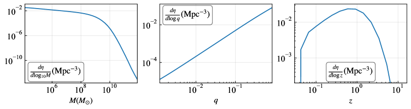
Figure S1: Comoving volumetric number density of SMBHBs for the fiducial model as a function of total SMBH mass $\displaystyle M$ (left), mass ratio $\displaystyle q$ (middle), and redshift $\displaystyle z$ (right).

For the data analysis, we allow the overall normalization of $\displaystyle h_{c}^{2}$ to vary as a nuisance parameter, denoted by $\displaystyle N$, which accounts for uncertainties in the population model. This parameter is assigned a prior based on the astrophysical priors listed in Table 1 that contribute to the normalization. Specifically, for each case, we calculate the corresponding $\displaystyle h_{c}^{2}$ for circular orbits driven solely by GW emission, and compare it to that of the fiducial model, defining the ratio as $\displaystyle N$. The distribution of $\displaystyle N$ is shown in Fig. S2, which can be modeled as $\displaystyle\log_{10}N=\mathcal{N}(-1.46,1.09)$.

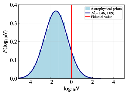
Figure S2: Distribution of the normalization factor $\displaystyle N$, defined as the ratio between the $\displaystyle h_{c}^{2}$ magnitude resulting from SMBHB population models (based on astrophysical priors) and the fiducial value in Table 1, without accounting for environmental hardening and eccentricities. The distribution is fit as $\displaystyle\log_{10}N=\mathcal{N}(-1.46,1.08)$, and used as the prior for normalization in data analysis. The fiducial value, fixed at $\displaystyle N=1$, is shown by the red line.

VII Statistics

In our data analysis, we estimate the posterior distribution of $\displaystyle\log_{10}\rho_{\rm pc}$, $\displaystyle\gamma$, $\displaystyle e_{0}$ and $\displaystyle\log_{10}N$. This can be separated into two components:

$$P\left(\log_{10}\frac{\rho_{\rm pc}/10^{5}}{M_{\odot}/{\rm pc}^{3}},\gamma,e_{0},\log_{10}N|\bm{\delta}t\right)$$ (S17)

$$= \int\prod_{k}{\rm d}\log_{10}h_{c}^{2}(f_{k})\,P\left(\log_{10}\frac{\rho_{\rm pc}/10^{5}}{M_{\odot}/{\rm pc}^{3}},\gamma,e_{0},\log_{10}N|\{\log_{10}h_{c}^{2}(f_{k})\}\right)\times P\left(\{\log_{10}h_{c}^{2}(f_{k})\}|\bm{\delta t}\right),$$

where $\displaystyle\bm{\delta t}$ represents the timing residual data from the NANOGrav 15-year dataset [5], and $\displaystyle f_{k}=k/T_{\rm obs}$ denotes the frequencies indexed by $\displaystyle k=1,\,2,\,3,\,4,\,5$, corresponding to the five lowest frequency bins, with $\displaystyle T_{\rm obs}\approx 16$ years as the observation time.

The second term in Eq. (S17) represents the posterior distributions of the free spectrum GWs derived by the NANOGrav collaboration [10]. The first term is calculated using Bayes’ theorem:

$$P\left(\log_{10}\frac{\rho_{\rm pc}/10^{5}}{M_{\odot}/{\rm pc}^{3}},\gamma,e_{0},\log_{10}N|\{\log_{10}h_{c}^{2}(f_{k})\}\right)$$ (S18)

$$\propto P\left(\{\log_{10}h_{c}^{2}(f_{k})\}|\log_{10}\frac{\rho_{\rm pc}/10^{5}}{M_{\odot}/{\rm pc}^{3}},\gamma,e_{0},\log_{10}N\right)P\left(\log_{10}\frac{\rho_{\rm pc}/10^{5}}{M_{\odot}/{\rm pc}^{3}}\right)P\left(\gamma\right)P\left(e_{0}\right)P\left(N\right),$$

The first term is computed in Sec. V, where Poisson fluctuations are neglected. The remaining terms are the priors for each parameter:

$$P\left(\log_{10}\frac{\rho_{\rm pc}/10^{5}}{M_{\odot}/{\rm pc}^{3}}\right)=U[-4,4],$$ (S19)

$$P\left(\gamma\right)=U[0,2.4],$$

$$P\left(e_{0}\right)=U[0,0.999],$$

$$P\left(N\right)=\mathcal{N}(-1.46,1.09).$$

where the prior for $\displaystyle N$ is calculated in Sec. VI.

For practical implementation, we use PTArcade [90], based on ceffyl [91], to model the prior distributions and fit the results to the free spectrum data.