From CNN to ConvRNN: Adapting Visualization Techniques for Time-Series Anomaly Detection

Abstract

Nowadays, neural networks are commonly used to solve various problems. Unfortunately, despite their effectiveness, they are often perceived as black boxes capable of providing answers without explaining their decisions, which raises numerous ethical and legal concerns. Fortunately, the field of explainability helps users understand these results. This aspect of machine learning allows users to grasp the decision-making process of a model and verify the relevance of its outcomes. In this article, we focus on the learning process carried out by a “time distributed“ convRNN, which performs anomaly detection from video data.

Keywords: Deep learning, Explicability, Visualization, Time Distributed Convolution, Saliency, Grad Cam

1 Introduction

Deep neural networks play a key role today in solving complex problems, particularly in real-time anomaly detection from videos. However, their opaque nature makes them “black boxes” that are difficult to interpret, which raises not only technical but also ethical and legal challenges. This opacity is particularly problematic when it comes to justifying decisions made by these systems, especially in sensitive domains like security, where anomalies such as fights, gunshots, or car accidents need to be detected. In this context, the European Union implemented the General Data Protection Regulation (GDPR) in May 2019, which imposes strict rules regarding the use of algorithms in decision-making. Article 22-1 of the GDPR states that a decision cannot be based solely on automated processing if it has significant effects on a person. This makes it even more crucial to develop techniques that explain and help understand the decisions made by anomaly detection models, particularly to ensure their legal and ethical compliance. In this study, we implemented a convRNN model to detect anomalies in videos. We focused our analysis on critical security actions such as fights or gunshots. Regarding explainability, it is much easier to interpret the features learned by our convolutional network, as they can be visualized, unlike those generated by our RNN. In projects employing convolutional networks for image processing, it is common to visualize the features extracted by the model to assess the relevance of its learning. However, video data processing complicates this approach. Given that a video essentially consists of a sequence of images, it is legitimate to question whether the same visualization techniques can be applied to models incorporating “time distributed“ convolutions. This question is particularly important in the context of anomaly detection, where understanding the areas on which the model focuses its attention is essential. To address this issue, we begin by reviewing the main visualization techniques available for neural networks, particularly in the context of image and video analysis. Next, we detail the procedure we adopted to apply these techniques to our “time distributed“ convRNN model. Finally, we present our results and discuss their implications before concluding.

2 Related work

In 2019, Christoph Molnar published a book titled A Guide for Making Black Box Models Explainable, which highlighted various explainability and visualization technologies [8]. On the one hand, some technologies, such as LIME (Local Interpretable Model-Agnotic Explanations), proposed on August 9, 2016, by Marco Tulio Ribeiro, Sameer Singh, and Carlos Guestrin [12], or SHAP (SHapley Additive exPlanations), proposed in November 2017 by Scott M. Lundberg and Su-In Lee, [7] are independent of the model used. On the other hand, some technologies are specific to certain models, such as convolution networks, for which one can find visualization techniques like convolution filters [5], saliency maps [15, 14], activation maps [13, 1, 16], etc.

Many libraries exist to help users visualize these characteristics. In 2017, Kotikalapud Raghavendra proposed keras-vis [6], a public library allowing users to visualize the convolution filters of each layer, their evolution during training, and activation maps. Later, in 2020, Philippe Remy developed another library, called keract[11], to perform similar processing. Also in 2020, Gotkowski, Karol et al. proposed another library, which allowed users to visualize both 2D and 3D attention maps [4]. Nowadays, the keras library developed by François Chollet in 2015 [3] also includes some of these visualization techniques.

3 Approach

Our model was developed using the Keras library. For the convolutional component, we chose VGG19, and for the sequential component, we used GRU. To add a temporal dimension to our data, we encapsulated VGG19 within a “Time Distributed“ layer. The role of this layer is to apply the same processing to each element of a data sequence—in our case, to apply VGG19 to each image, in order to integrate a temporal dimension before passing the information to the GRU for sequential analysis. A diagram of our architecture is presented in figure 1.

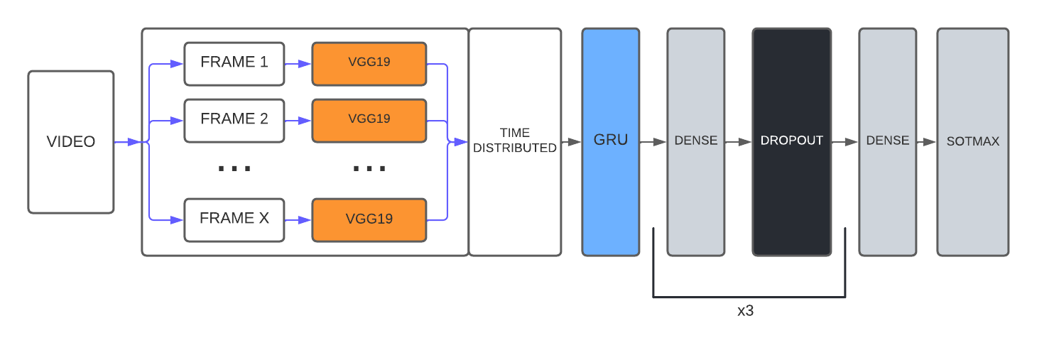
Figure 1: Model Architecture

In this study, we chose to focus on explainability techniques such as Grad-CAM, saliency maps, feature maps, and filter visualization. The use of these methods allows for a more direct and immediate understanding of the internal mechanisms of our model, thereby facilitating the interpretation of results. Additionally, by avoiding external dependencies, we ensure consistency and reproducibility in our analyses. Unfortunately, we observed that visualization libraries specifically designed for CNNs were not well-suited to our type of architecture. The first problem lies in the structure of our model. In a standard network using 2D or 3D convolutional layers, the layers are directly connected to each other. However, in our architecture, the convolution is encapsulated within a ”Time Distributed” layer, which implies the presence of a sub-model within this layer, as illustrated in figure 2. This sub-model is indirectly connected to other layers, making the propagation of information and gradients through the network more complex. The second problem involves the addition of the temporal dimension. Unlike models that process images or 3D objects, which generate an output visualization for a single input, in our case, we are processing videos. This means we have multiple input images for a single output visualization, which must represent the entire input sequence.

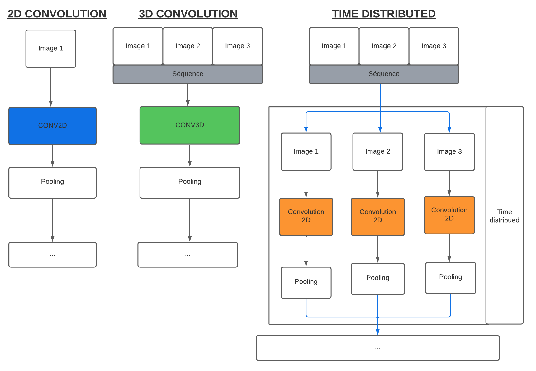
Figure 2: Architecture Comparison: 2D convolution / 3D convolution / Time distributed convolution

Our goal is therefore to create a visualization for each image in order to better understand the processing performed by our sub-model while adhering to GDPR requirements. We aim to visualize the areas where the model focuses its attention when predicting an anomaly. For this, it is possible to use saliency maps and activation maps. Saliency maps highlight the pixels of interest in an image, while activation maps provide a visualization of the different regions of the image that contribute to the final prediction. Saliency maps are generated by calculating the gradient of the activation with respect to our input data, whereas activation maps are obtained by calculating the gradient of the activation with respect to the output of the layer we wish to visualize. To create these visualizations, information needs to be propagated through the network to obtain the final activation. Unfortunately, the use of a ”Time Distributed” layer complicates the propagation between the sub-model and the main model. Moreover, extracting the sub-model severs the connection with the subsequent layers. The generation of saliency maps requires calculating the gradient from a sequence rather than an individual image, which results in a series of gradients corresponding to the sequence length. These gradients are then displayed, providing a saliency map for each image. For activation maps, the solution we found is to exploit the output of the ”Time Distributed” layer. As mentioned earlier, this layer adds a temporal factor to the data by applying the same treatment to each image in the sequence. The output of this layer can be interpreted as a list of results, with one result for each image. The calculated gradients have the same dimensions as this output, which allows each gradient to be applied to its corresponding output and to generate an activation map, which is then projected onto the associated image. It should also be noted that with this type of architecture, it is only possible to generate activation maps for the output layer of our sub-model.

4 Experimentation:

In this section, we will present our results as well as the advantages and disadvantages of each of the approaches explained earlier. For a non-expert, such as a security officer, it is much more practical to rely on activation maps rather than saliency maps, as demonstrated in figures 4 and 4.

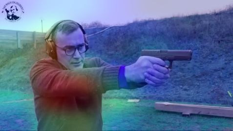
Figure 3: Activation maps

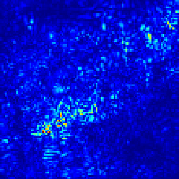
Figure 4: Saliency maps

By examining the activation maps presented in Figure 5, we can observe that our model does not focus on the same areas from one image to another, even when the images are consecutive. This is due to the lack of an attention layer in our model.

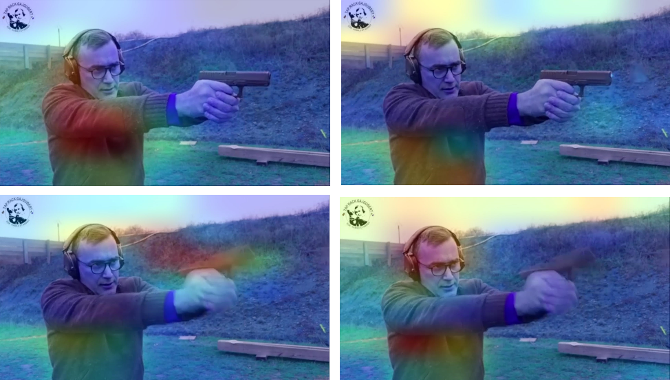
Figure 5: Class activation map (Grad-CAM) for a shooting video

To facilitate the interpretation of our sequences, we used OpenCV to extract the contours of these activation maps. This contour visualization (see Figure 6) allowed us to notice areas of low activation that are difficult to perceive via the activation maps. However, it has some drawbacks; for instance, the contour detection is not very precise, and there may be contours included within others when there is a major activation area surrounded by minor ones. Additionally, at present, this new visualization does not allow us to know the intensity of the activations. Figures 7 perfectly illustrate the advantages and disadvantages of this technique. In image number 1, we can see that the gun is perceived as a low-activation area, which is hard to see on the activation map but becomes very clear through the contours. We can also observe a major activation area surrounded by a minor one located on the left side of the image. Image number 2 shows a person hitting another. With the activation map, it seems that the model perceives the action well but mistakenly labels the scene as ”Normal.” However, by visualizing the contours, we realize that it completely misses the action.

Figure 6: Example of visualization for classes: shooting and fight

Figure 7: Activation map + contours visualization perform on images extracted from shooting / fight videos.

The activation maps presented in Figures 8, 9, and 10 also allowed us to observe the influence that other layers (RNN, Dense, Dropout) have on the features learned by our convolution. This influence is caused by the backpropagation performed in this type of model, which enabled us to better define the parameters of these layers.

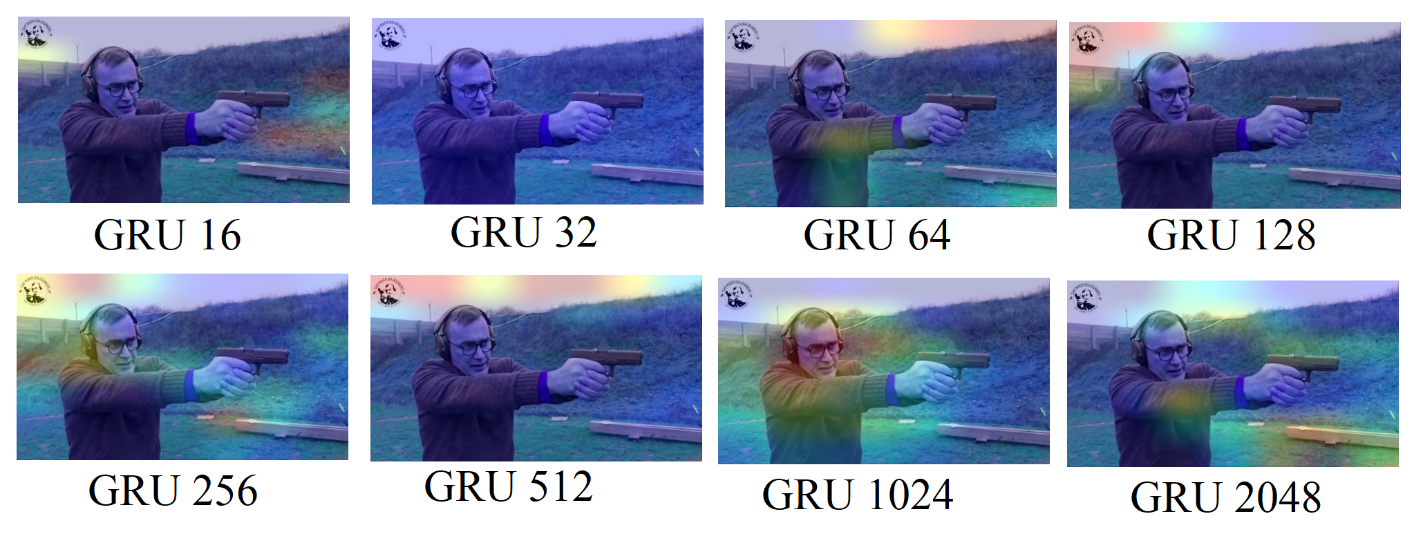
Figure 8: Activation map with variation of the number of neurons in the GRU Layer.

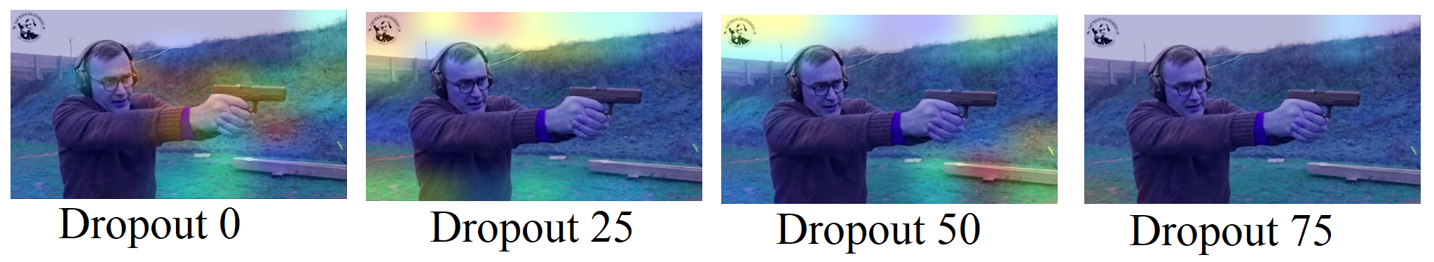
Figure 9: Activation map showing the variation of the dropout.

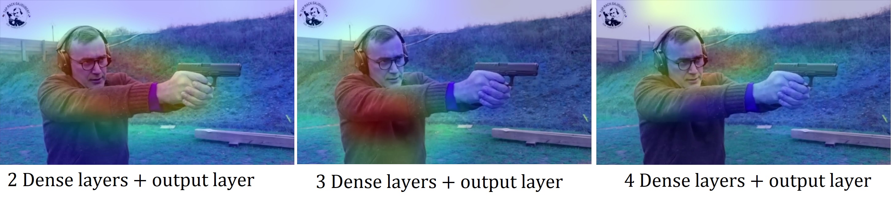
Figure 10: Activation map showing the variation of dense layer in the MLP.

These visualizations also allow for the examination of the characteristics associated with the ’normal’ class. In a supervised learning context, this class represents the absence of anomalies, encompassing a wide range of actions such as working, walking, or exercising, among others. It is interesting to note that movements in this class are often slow, in contrast to anomalies, which are marked by abrupt and rapid movements. While a human would default to assigning the normal class in the absence of anomaly indicators, our model does not follow this logic. To predict the normal class, it must detect specific features that represent it. By visualizing examples of videos belonging to this class through activation maps 11, saliency maps 12, or feature maps 13, we found that our model primarily relies on the posture of the individuals present on screen to predict this class.

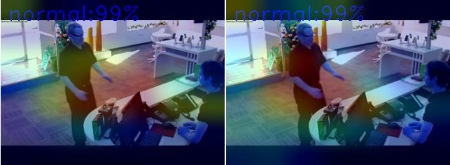
Figure 11: Activation Map for a normal video

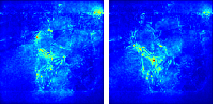
Figure 12: Saliency map for a normal video

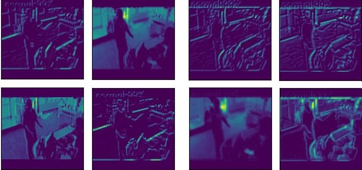
Figure 13: 8 convolution filters extracted for a normal video

5 Conclusion

Through this article, we have demonstrated the possibility of adapting certain visualization techniques specific to convolutional neural networks (CNNs) for use with convolutional recurrent networks (convRNNs), integrating convolutions within a“Time Distributed“ layer, while complying with GDPR requirements.

However, several avenues remain to be explored:

1. The visualization of contours could be improved by incorporating a representation of the intensity of activation zones.

2. Another promising approach would be to leverage object detection models to precisely locate anomalies, which could facilitate real-time visualizations, representing a major advantage for applications where time is a critical factor. While vision transformers allow visualizations using attention maps, this process remains slow and computationally expensive, making it unsuitable for applications requiring immediate feedback.

3. The development of visualization techniques specifically tailored to video data could significantly enrich our analytical capabilities.

With the advancement of artificial intelligence, explainability has become a major issue that has generated significant interest within the scientific community. This interest has led to numerous studies conducted each year, particularly concerning convolutional networks or image processing [10, 9, 2, 17]. These ongoing research efforts contribute to clarifying and improving our understanding of this field, paving the way for increasingly transparent and interpretable AI systems.

References

- [1] C Aditya, S Anirban, D Abhishek, and H Prantik. Grad-cam++: Improved visual explanations for deep convolutional networks. arxiv 2018. arXiv preprint arXiv:1710.11063.
- [2] David Bau, Jun-Yan Zhu, Hendrik Strobelt, Agata Lapedriza, Bolei Zhou, and Antonio Torralba. Understanding the role of individual units in a deep neural network. Proceedings of the National Academy of Sciences, 2020.
- [3] Francois Chollet et al. Keras, 2015.
- [4] Karol Gotkowski, Camila Gonzalez, Andreas Bucher, and Anirban Mukhopadhyay. M3d-cam: A pytorch library to generate 3d data attention maps for medical deep learning. arXiv preprint arXiv:2007.00453, 2020.
- [5] Peng-Tao Jiang, Chang-Bin Zhang, Qibin Hou, Ming-Ming Cheng, and Yunchao Wei. Layercam: Exploring hierarchical class activation maps for localization. IEEE Transactions on Image Processing, 30:5875–5888, 2021.
- [6] Raghavendra Kotikalapudi and contributors. keras-vis. https://github.com/raghakot/keras-vis, 2017.
- [7] Scott M Lundberg and Su-In Lee. A unified approach to interpreting model predictions. Advances in neural information processing systems, 30, 2017.
- [8] Christoph Molnar. Interpretable Machine Learning. 2019.
- [9] Chris Olah, Alexander Mordvintsev, and Ludwig Schubert. Feature visualization. Distill, 2017. https://distill.pub/2017/feature-visualization.
- [10] Chris Olah, Arvind Satyanarayan, Ian Johnson, Shan Carter, Ludwig Schubert, Katherine Ye, and Alexander Mordvintsev. The building blocks of interpretability. Distill, 2018. https://distill.pub/2018/building-blocks.
- [11] Philippe Remy. Keract: A library for visualizing activations and gradients. https://github.com/philipperemy/keract, 2020.
- [12] Marco Tulio Ribeiro, Sameer Singh, and Carlos Guestrin. ” why should i trust you?” explaining the predictions of any classifier. In Proceedings of the 22nd ACM SIGKDD international conference on knowledge discovery and data mining, pages 1135–1144, 2016.
- [13] Ramprasaath R Selvaraju, Michael Cogswell, Abhishek Das, Ramakrishna Vedantam, Devi Parikh, and Dhruv Batra. Grad-cam: Visual explanations from deep networks via gradient-based localization. In Proceedings of the IEEE international conference on computer vision, pages 618–626, 2017.
- [14] Karen Simonyan, Andrea Vedaldi, and Andrew Zisserman. Deep inside convolutional networks: Visualising image classification models and saliency maps. In In Workshop at International Conference on Learning Representations. Citeseer, 2014.
- [15] Daniel Smilkov, Nikhil Thorat, Been Kim, Fernanda Viégas, and Martin Wattenberg. Smoothgrad: removing noise by adding noise. arXiv preprint arXiv:1706.03825, 2017.
- [16] Haofan Wang, Zifan Wang, Mengnan Du, Fan Yang, Zijian Zhang, Sirui Ding, Piotr Mardziel, and Xia Hu. Score-cam: Score-weighted visual explanations for convolutional neural networks. In Proceedings of the IEEE/CVF conference on computer vision and pattern recognition workshops, pages 24–25, 2020.
- [17] Quanshi Zhang, Ying Nian Wu, and Song-Chun Zhu. Interpretable convolutional neural networks. In Proceedings of the IEEE conference on computer vision and pattern recognition, pages 8827–8836, 2018.